Alternating Shrinking Higher-order Interactions for Sparse Neural Population Activity

Abstract

Neurons in living things work cooperatively and efficiently to process incoming sensory information, often exhibiting sparse and widespread population activity involving structured higher-order interactions. While there are statistical models based on continuous probability distributions for neurons’ sparse firing rates, how the spiking activities of a large number of interacting neurons result in the sparse and widespread population activity remains unknown. Here, for homogeneous (0,1) binary neurons, we provide sufficient conditions under which their spike-count population distribution converges to a sparse widespread distribution of the population spike rate in an infinitely large population of neurons. Following the conditions, we propose new models belonging to an exponential family distribution in which the sign and magnitude of neurons’ higher-order interactions alternate and shrink as the order increases. The distributions exhibit parameter-dependent sparsity on a bounded support for the population firing rate. The theory serves as a building block for developing prior distributions and neurons’ non-linearity for spike-based sparse coding.

1 Introduction

The fundamental constraint placed on neural systems operating in natural environments is efficiency. Neurons therefore exhibit sparsity in various aspects of their activity patterns [1, 2] such as in the distribution of individual neuron responses to multiple stimuli (lifetime sparseness) [3] and the response distribution of a population of neurons (population sparseness) [3, 4, 5]. These sparse distributions require non-trivial higher-order statistical structure. For continuous distributions, sparsity is characterized by the higher-order moments such as kurtosis, which measures the tailedness of the distributions. Many parametric sparse distributions have been proposed, often within the context of the Bayesian prior for sparse coding [6]. Nevertheless, understanding how such distributions arise from the spiking activities of interacting neurons remains elusive.

One approach to understand cooperative spiking activities of neurons involves analyzing near-simultaneous activities by binarizing the spiking activity within short time windows. When expressed by the exponential family distributions with interactions of multiple orders, this analysis can reveal interactions among subsets of neurons in the population. Interactions among more than two neurons are often termed higher-order interactions (HOIs). The model that lacks HOIs is obtained by constructing a distribution that maximizes entropy while constraining activity rates of individual neurons and joint activity rates of neuron pairs. This model, in which all HOIs are fixed at zero, is called a pairwise maximum entropy (MaxEnt) model (a.k.a the spin-glass or Ising model in statistical physics and the Boltzmann machine in machine learning). The pairwise MaxEnt model highlights the role of HOIs. The joint activity of more than two neurons produced by this model appears as chance coincidences expected from the activity rates of individual neurons and neuron pairs. Consequently, if nonzero HOIs exist, they indicate deviations of the joint activities of more than two neurons from these chance coincidences.

There is considerable evidence suggesting that HOIs are necessary for characterizing the activity of neural populations. Early in vitro studies reported that the pairwise MaxEnt model accounted for approximately 90% of activity patterns of small populations [7, 8], implying that HOIs made only marginal contributions. However, HOIs may become more prominent as the population size increases [9, 10, 11, 12]. In fact, significant HOIs were later found ubiquitously both in vitro and in vivo neurons [13, 14, 11, 15, 16]. Analyzing HOIs enables researchers to uncover the underlying circuitry [17] and provides insights into their stimulus coding [18, 19, 14, 15, 20].

One of the most striking features related to higher-order interactions (HOIs) is the sparse yet widespread distribution of neural activity. Spike-count histograms for the number of simultaneously active neurons often exhibit widespread distributions, with notably longer tails for probabilities in highly synchronous states compared to independent or pairwise MaxEnt models [11, 15]. This underscores the importance of HOIs. Furthermore, the presence of highly variable probabilities leads to increased heat capacity (i.e., the variance of log probabilities). This indicates that the HOIs facilitate neural systems transitioning to highly fluctuating regimes, which may manifest as a critical state of the systems [21].

At the same time, spike-count distributions of neurons in various brain regions exhibit sparsity. Evidence for this can be appreciated in the spike-count histogram of individual neurons, such as retinal ganglion cells [22], V1 neurons [23], and primary auditory cortex neurons [24]. Population-level histograms of neural activity also display sparse profiles. Neurons are only sparsely active over time, with the duration of a state in which all neurons are silent being significantly longer than the prediction made by the pairwise MaxEnt model in both in vitro [10, 11, 16] and in vivo [15, 14, 25] studies. The study in [16] showed that the simultaneous silence is a dominant factor representing the HOIs, resulting in the alternating structure with positive pairwise, negative triple-wise, positive quadruple-wise interactions and so on when the activity is represented by $(0,1)$.

While it is evident that HOIs are involved in sparse, widespread distributions, their sufficient conditions and parametric models derived from them have not been proposed yet. In this work, we establish conditions for the sparse and widespread distributions for spiking activities of a homogeneous neural population and provide new parametric models belonging to the exponential family distribution based on the theory. The necessity of non-zero higher-order interactions in constructing the widespread distributions was also pointed out by Amari et al. [26]. As opposed to the previous study, we show that the base measure function in the exponential family distribution is an important factor in cancelling the entropy term of the combinatorial patterns that may otherwise dominate in the probability mass function. Further, since our theory makes it possible to construct the sparse widespread distributions belonging to the exponential family directly, we provide explicit models with structured higher-order interactions exhibiting parameter-dependent sparsity.

The paper is organized as follows. In the following section (Section 2), we describe a probability mass function (PMF) of $(0,1)$ binary patterns using the exponential family distribution, assuming homogeneity over the neurons, and construct a population-count histogram, a distribution of the total activity in the population. We provide sufficient conditions that make a distribution widespread with its peak at a population spike count of zero in the limit of an infinite number of neurons. Section 3 introduces our alternating shrinking higher-order interaction models, whose corresponding probability density functions (PDFs) become widespread and remain sparse in the limit of a large number of neurons. Then in Section 4, we present the scenario when entropy in the PMF dominates in a large number of neurons, which hinders the widespread property. We conclude with a discussion in Section 5.

2 Homogeneous sparse population of neurons

The activity of $N$ neurons is represented by a set of binary random variables, using a column vector, $\mathbf{X}=[X_{1},X_{2},\ldots,X_{N}]^{\textsf{T}}$ where $X_{i}\in\{0,1\}$ and for which we assume stationarity. The $i$th neuron activity $X_{i}$ is $1$ if the neuron is active and $0$ otherwise. The probabilities of generating binary activity patterns, specified by $\mathbf{x}=[x_{1},x_{2},\ldots,x_{N}]^{\textsf{T}}$, where $x_{i}\in\{0,1\}$ are given as $\mathcal{P}\left(\mathbf{X}=\mathbf{x}\right)$. This PMF can be written in the form of an exponential family distribution given by

$$\mathcal{P}\left(\mathbf{X}=\mathbf{x}\right) =\frac{h\left(\mathbf{x}\right)}{Z}\exp\left[\sum\limits_{i=1}^{N}\theta_{i}x_{i}+\sum\limits_{i_{1}<i_{2}}\theta_{i_{1}i_{2}}x_{i_{1}}x_{i_{2}}+\sum\limits_{i_{1}<i_{2}<i_{3}}\theta_{i_{1}i_{2}i_{3}}x_{i_{1}}x_{i_{2}}x_{i_{3}}\right.$$

$$\phantom{======================}+\ldots+\theta_{12\ldots N}x_{i_{1}}\ldots x_{i_{N}}\Bigg{]},$$ (1)

where $Z$ is a normalization term, and the parameters $\{\theta_{i}\}_{i=1}^{N}$, $\{\theta_{i_{1}i_{2}}\}_{i_{1}<i_{2}}$, $\ldots$, $\theta_{1\ldots N}$ are called natural parameters. They characterize interactions among subset neurons indicated by the subscripts [27, 28]. The exponential family distribution allows the base measure function $h\left(\mathbf{x}\right)$ to be a general nonnegative function of the vector pattern $\mathbf{x}$. Here we will assume that $h\left(\mathbf{x}\right)$ is a function of the total activity, $\sum_{i=1}^{N}x_{i}$. Although Eq. 1 can realize arbitrary probabilities for all possible patterns even if $h\left(\mathbf{x}\right)=1$, as we will show, the introduction of an appropriate base measure function simplifies the conditions for the sparse widespread distributions and for modelling the neural interactions. For simplicity, we use $\mathcal{P}\left(\mathbf{x}\right)$ to represent $\mathcal{P}\left(\mathbf{X}=\mathbf{x}\right)$.

We study the activity of a population of homogeneous neurons. Homogeneity on its own is an important assumption for which specific preference over some neural activity patterns is ignored. Nonetheless, homogeneity allows us to change the analysis focus from a local to a global view on the sparse neural population activity in a region, which in turn facilitates the identification of theoretical properties. The binary activity of the homogeneous population is described by using single parameters $\theta_{k}$ ($k=1,2,\ldots,N$) for all the combinatorial $k$-th order interactions in Eq. (1)

$$\mathcal{P}\left(\mathbf{x}|\boldsymbol{\theta}_{N}\right)= \frac{h\left(\sum_{i=1}^{N}x_{i}\right)}{Z}\exp\left[\theta_{1}\sum_{i=1}^{N}x_{i}+\theta_{2}\sum_{i_{1}<i_{2}}x_{i_{1}}x_{i_{2}}+\ldots+\theta_{N}x_{i_{1}}x_{i_{2}}\ldots x_{i_{N}}\right],$$ (2)

where $\boldsymbol{\theta}_{N}=(\theta_{1},\theta_{2},\ldots,\theta_{N})$. This model extends the theoretical work by Amari et al. [26], where $h\left(\sum_{i=1}^{N}x_{i}\right)=1$. The population activity of the homogeneous neurons is characterized by the distribution of the number of active neurons in the population. For homogeneous neurons any individual binary pattern where $n$ neurons are active has the same probability. Therefore, the probability of having $n$ number of active neurons in the population is given by

$$\mathcal{P}\left(\sum_{i=1}^{N}X_{i}=n|\boldsymbol{\theta}_{N}\right)= \left(\begin{array}[]{c}N\\ n\end{array}\right)\mathcal{P}\left(x_{1}=1,\ldots,x_{n}=1,x_{n+1}=0,\ldots,x_{N}=0\;|\;\boldsymbol{\theta}_{N}\right)$$ (5)

$$= \left(\begin{array}[]{c}N\\ n\end{array}\right)\frac{h\left(n\right)}{Z}\exp\left[\left(\begin{array}[]{c}n\\ 1\end{array}\right)\theta_{1}+\left(\begin{array}[]{c}n\\ 2\end{array}\right)\theta_{2}+\ldots+\left(\begin{array}[]{c}n\\ n\end{array}\right)\theta_{n}\right]$$ (14)

$$= \left(\begin{array}[]{c}N\\ n\end{array}\right)\frac{h\left(n\right)}{Z}\exp\left[\sum_{k=1}^{n}\left(\begin{array}[]{c}n\\ k\end{array}\right)\theta_{k}\right].$$ (19)

Let the fraction of active neurons (or population rate) be $R_{N}=\frac{1}{N}\sum_{i=1}^{N}X_{i}$. Using Eq. (19), the PMF of the random variable $R_{N}$, $\mathcal{P}\left(R_{N}=r_{N}|\boldsymbol{\theta}_{N}\right)$, where $r_{N}\in S_{r}$ with $S_{r}\equiv\left\{0,\frac{1}{N},\frac{2}{N},\ldots,1\right\}$, is

$$\mathcal{P}\left(R_{N}=r_{N}|\boldsymbol{\theta}_{N}\right)= \mathcal{P}\left(\left.\sum_{i}X_{i}=Nr_{N}\right|\boldsymbol{\theta}_{N}\right)$$

$$= \left(\begin{array}[]{c}N\\ Nr_{N}\end{array}\right)\frac{h\left(Nr_{N}\right)}{Z}\exp\left[\sum_{k=1}^{Nr_{N}}\left(\begin{array}[]{c}Nr_{N}\\ k\end{array}\right)\theta_{k}\right].$$ (24)

We call this a PMF of the discrete population rate and we rewrite it as

$$\mathcal{P}\left(R_{N}=r_{N}|\boldsymbol{\theta}_{N}\right)= \frac{1}{Z}\exp\left[NG_{N}(r_{N};\boldsymbol{\theta}_{N})\right],$$ (25)

where

$$G_{N}\left(r_{N};\boldsymbol{\theta}_{N}\right)=\frac{1}{N}\log\left(\begin{array}[]{c}N\\ Nr_{N}\end{array}\right)+\frac{1}{N}\log h\left(Nr_{N}\right)+\frac{1}{N}Q_{N}\left(r_{N};\boldsymbol{\theta}_{N}\right),$$ (28)

and with the polynomial term defined as

$$Q_{N}\left(r_{N};\boldsymbol{\theta}_{N}\right)=\sum_{k=1}^{Nr_{N}}\left(\begin{array}[]{c}Nr_{N}\\ k\end{array}\right)\theta_{k}.$$ (29)

We note that the new underlying base measure function for such population rate distribution (Eq. (24)) consists of the binomial term multiplied by the $h\left(\cdot\right)$ function, i.e., $\left(\begin{array}[]{c}N\\ Nr_{N}\end{array}\right)h\left(Nr_{N}\right)$. As we stated before, such base measure function could alternatively be represented in a different way inside the (possibly non-polynomial) function $Q_{N}\left(\cdot\right)$ as a function of the active neurons given the canonical parameters. Nonetheless, the representation we chose facilitates analysis in the limit of an infinitely large population of neurons as we will see. In the following, we use $\mathcal{P}\left(r_{N}|\boldsymbol{\theta}_{N}\right)$ to represent the PMF above.

We are interested in the behaviour of the PMF (Eq. (25)) in the limit of a large number of neurons ($N\rightarrow\infty$): Namely, the probability density function (PDF) given through the relation $p\left(r|\boldsymbol{\lambda}\right)dr=\lim_{N\to\infty}\mathcal{P}\left(r_{N}|\boldsymbol{\theta}_{N}\right)$, where $r$ is the continuous population rate defined in the support $[0,1]$ and $\boldsymbol{\lambda}$ is the set of parameters for the PDF. We wish to know the conditions with which this PDF is sufficiently concentrated near its peak at $0$. Such a PDF would be relevant to model experimentally observed sparse population activity across different cortical populations, where arbitrarily low firing rates were exhibited by most neurons [29]. Following Amari et al.’s framework to construct wide spread distributions [26], we provide a new theorem below with the sufficient conditions for having a sparse and widespread distribution.

Theorem 1

Let $G_{N}\left(r_{N};\boldsymbol{\theta}_{N}\right)$ be a non-positive strictly decreasing function with finite values for $r_{N}\in S_{r}$. If $NG_{N}\left(r_{N};\boldsymbol{\theta}\right)$ has the following order of magnitude in terms of $N$,

$$\mathcal{O}\left(NG_{N}\left(r_{N};\boldsymbol{\theta}_{N}\right)\right)=\mathcal{O}\left(1\right),$$ (30)

then the corresponding probability density function given through $\;p\left(r|\boldsymbol{\lambda}\right)dr=\lim_{N\to\infty}\ \mathcal{P}\left(r_{N}|\boldsymbol{\theta}_{N}\right)\;$ is widespread in $(0,1]$ with a single non-concentrated maximum at $0$.

For a proof, the reader can refer to A.1.

Specifically, if we have the following form for the function $h(\mathbf{x})$:

$$h\left(\sum{}_{i=1}^{N}x_{i}\right) =1\left/\left(\begin{array}[]{c}N\\ \sum_{i=1}^{N}x_{i}\end{array}\right)\right.$$ (33)

then the first two terms in Eq. (28) cancel out, resulting in

$$G_{N}\left(r_{N};\boldsymbol{\theta}_{N}\right)=\frac{1}{N}Q_{N}\left(r_{N};\boldsymbol{\theta}_{N}\right).$$ (34)

Thus we obtain the following corollary

Corollary 1

Let $h(\mathbf{x})$ be given by Eq. (33). If the polynomial term $Q_{N}\left(r_{N};\boldsymbol{\theta}_{N}\right)$ satisfies

$$\mathcal{O}\left(Q_{N}\left(r_{N};\boldsymbol{\theta}_{N}\right)\right)=\mathcal{O}\left(1\right),$$ (35)

and if $q\left(r;\boldsymbol{\lambda}\right)=\lim_{N\to\infty}Q_{N}\left(r_{N};\boldsymbol{\theta}_{N}\right)$ is a non-positive strictly decreasing function, then the probability density function $p\left(r|\boldsymbol{\lambda}\right)$ is widespread in $(0,1]$ with a single non-concentrated maximum at $0$.

Here we introduce the simplest homogeneous model able to produce sparse population activity, i.e., a homogeneous population of independent binary neurons with only the first-order parameters ($\theta_{2}=\theta_{3}=\ldots=\theta_{N}=0$). Using $\theta_{1}=-\mathpzc{f}/N$, the binary population PMF of the independent homogeneous neurons is given as

$$\mathcal{P}\left(\mathbf{x}|\mathpzc{f}\right)=\frac{h\left(\sum{}_{i=1}^{N}x_{i}\right)}{Z}\exp\left[-\mathpzc{f}\frac{\sum{}_{i=1}^{N}x_{i}}{N}\right],$$ (36)

where we assume that $\mathpzc{f}>0$ and the function $h\left(\cdot\right)$ is given by Eq. (33). With this $h\left(\cdot\right)$ function that cancels out with the binomial term in Eq. (28), the corresponding population rate PMF (Eq. (25)) is given as

$$\mathcal{P}\left(r_{N}|\theta_{1}\right) =\frac{1}{Z}e^{-\mathpzc{f}r_{N}}.$$ (37)

The corresponding continuous PDF is obtained through

$$p\left(r|f\right)dr=\lim_{N\to\infty}\mathcal{P}\left(r_{N}|\theta_{1}\right)=\frac{1}{Z}e^{-\mathpzc{f}r}dr,$$ (38)

where the normalization constant is obtained as

$$Z=\int_{0}^{1}e^{-\mathpzc{f}r}dr=\frac{1-e^{-\mathpzc{f}}}{\mathpzc{f}}.$$ (39)

Since $\mathcal{O}\left(-\mathpzc{f}r_{N}\right)=\mathcal{O}\left(1\right)$ and $q\left(r;\mathpzc{f}\right)=-fr$ is a strictly decreasing function, the PDF in Eq. (38) is widespread in $(0,1]$ with a single non-concentrated maximum at $0$ (Corollary 1). The sparsity in such PDF is controlled by the $\mathpzc{f}$ parameter. See the A.2 for the mean and the variance of the distribution.

This density corresponds to the PDF of an exponential distribution with parameter $\mathpzc{f}>0$ but with a compact support in $[0,1]$, instead of the support in $[0,\infty)$. This independent model serves as a baseline in investigating the effect of the pairwise and higher-order interactions in shaping the sparse distribution.

In the next section (Section 3), we present our proposed model whose population rate PMF is a particular case of Eq. (25). The distribution satisfies the conditions in Theorem 1 and converges to a widespread continuous distribution with parameter-dependent sparsity. In the subsequent section (Section 4), we present a case to which Theorem 1 does not apply, resulting in a concentrated distribution.

3 The model with alternating and shrinking higher-order interactions

Neuronal populations exhibit significant excess rate of simultaneous silence [14, 10, 11, 16], where all neurons become inactive, compared to the chance level predicted by the pairwise MaxEnt models. When expressed in $(0,1)$ patterns, the probability of silence of all neurons are captured by the feature given by $\prod_{i=1}^{N}(1-x_{i})$ using the exponential family distribution. The expansion of this feature leads to the HOIs with alternating signs for each order, which was proposed as a model of the simultaneous silence [16]. However, the simultaneous silence model is limited in that it captures only a state of total silence, whose measure becomes negligibly small for large number of neurons. Furthermore, as we show later, it is important to consider the shrinking strength in interactions as the order increases. The shrinking strength in interactions facilitates all orders of interaction to exist in the limit of a large number of neurons despite the alternating structure.

To construct the sparse model applicable to large $N$ limit, we consider the following distribution for the activity patterns of the homogeneous population of binary neurons:

$$\mathcal{P}(\mathbf{x}|\boldsymbol{\omega})=\frac{h\left(\sum_{i=1}^{N}x_{i}\right)}{Z}\exp\left[-\mathpzc{f}\sum_{j=1}^{N}\left(-1\right)^{j+1}C_{j}\left(\frac{\sum_{i=1}^{N}x_{i}}{N}\right)^{j}\right],$$ (40)

where $\boldsymbol{\omega}=\left\{\mathpzc{f},C_{1},C_{2},\ldots,C_{N}\right\}$ is the set of parameters and $Z$ is its partition function. We assume that $\mathpzc{f}>0$ and $C_{j}$ are positive ($C_{j}>0$) and decreasing with respect to $j$, $C_{j}<C_{j-1}\;\;\forall j=2,...,N$. In combination with $\left(-1\right)^{j+1}$, such coefficients impose an alternating structure whose magnitude shrinks as the order of interaction increases. We will provide specific choices of $C_{j}$ that make the alternating terms in the exponent converge to a decreasing function with respect to $r_{N}$. In this model, we use Eq. (33) for the base measure function $h(\mathbf{x})$. Using such function is one of the sufficient conditions required for the distribution to become widespread in the limit of a large number of neurons (Theorem 1). For a counter-example please see Section 4. Therefore, the population rate PMF becomes (see Eq. (34))

$$\mathcal{P}\left(r_{N}|\boldsymbol{\theta}_{N}\right)= \frac{1}{Z}\exp\left[Q_{N}\left(r_{N};\boldsymbol{\theta}_{N}\right)\right],$$ (41)

where $Q_{N}\left(r_{N};\boldsymbol{\theta}_{N}\right)$ is a polynomial given by Eq. (29), which will be calculated as follows.

The canonical form of the homogeneous population activity is given by Eq. (2). From Eq. (40), the canonical parameters ($\theta_{k}$, with interaction of the order $k$) of the alternating and shrinking interaction model are computed as

$$\theta_{1}= \sum_{l=1}^{N}\left(-1\right)^{l}\frac{\mathpzc{f}C_{l}}{N^{l}},$$

$$\theta_{2}= \sum_{l=2}^{N}\left(-1\right)^{l}\frac{\mathpzc{f}C_{l}}{N^{l}}\sum\limits_{\begin{subarray}{c}k_{1}+k_{2}=l\\ k_{1}>0,k_{2}>0\end{subarray}}\left(\begin{array}[]{c}l\\ k_{1},k_{2}\end{array}\right),$$ (44)

$$\theta_{3}= \sum_{l=3}^{N}\left(-1\right)^{l}\frac{\mathpzc{f}C_{l}}{N^{l}}\sum\limits_{\begin{subarray}{c}k_{1}+k_{2}+k_{3}=l\\ k_{1}>0,k_{2}>0,k_{3}>0\end{subarray}}\left(\begin{array}[]{c}l\\ k_{1},k_{2},k_{3}\end{array}\right),$$ (47)

$$\vdots$$

$$\theta_{N}= \left(-1\right)^{N}\frac{\mathpzc{f}C_{N}}{N^{N}}N!.$$ (48)

See the B.1 for the detailed derivation.

The PMF of the discrete population rate (Eq. (41)), will be specified by using these canonical parameters, $\boldsymbol{\theta}_{N}=(\theta_{1},\ldots,\theta_{N})$, where these parameters appear in the polynomial term, $Q_{N}\left(r_{N};\boldsymbol{\theta}_{N}\right)$ (Eq. (29)). Consequently, the polynomial term is computed as

$$Q_{N}\left(r_{N};\boldsymbol{\theta}_{N}\right) =-\mathpzc{f}\sum\limits_{j=1}^{Nr_{N}}\left(-1\right)^{j+1}C_{j}\left(r_{N}\right)^{j}+\mathcal{O}\left(\frac{1}{N}\right).$$ (49)

See B.2 for the derivation.

In the limit of $N\rightarrow\infty$, our population rate PMF becomes the continuous density given by (see B.3)

$$\lim_{N\rightarrow\infty}\mathcal{P}\left(r_{N}|\boldsymbol{\theta}_{N}\right) =p\left(r|\boldsymbol{\lambda}\right)dr$$

$$=\frac{1}{Z}\exp\left[-\mathpzc{f}\sum_{j=1}^{\infty}\left(-1\right)^{j+1}C_{j}r^{j}\right]dr,$$ (50)

where $\boldsymbol{\lambda}=\left\{\mathpzc{f},\left\{C_{j}\right\}_{j\in\mathbb{N}^{+}}\right\}$. Depending on the choice of each $C_{j}$, we obtain different types of densities. Here we provide two examples where the polynomial term $Q_{N}\left(r_{N};\boldsymbol{\theta}_{N}\right)$ converges to a non-positive decreasing function with respect to $r$, and therefore the corresponding densities result in widespread distributions with a non-concentrated maximum at 0 (Corollary 1).

Polylogarithmic exponential distribution If we define $C_{j}=\frac{1}{j^{m}}\;\;\forall j\;\;$ then the probability density function in Eq. (50) is

$$p\left(r|\mathpzc{f},m\right)=\frac{1}{Z}\exp\left[\mathpzc{f}\text{Li}_{m}\left[-r\right]\right],$$ (51)

where $\text{Li}_{m}[\cdot]$ is the polylogarithm function of order $m=1,2,3,\ldots$ (See B.3). We call the density in Eq. (51) the polylogarithmic exponential density, where the function $\mathpzc{f}\text{Li}_{m}\left[-r\right]$ is non-positive (see C.1) and strictly decreasing (see C.2) for $r\in[0,1]$ with a maximum at $r=0$. See Fig. 1 for the density functions for different $\mathpzc{f}$ and $m$. Note that $m=1$ we obtain the natural logarithm, i.e.,

$$\text{Li}_{1}\left[-r\right]=-\log\left[1+r\right].$$ (52)

Figure 1: Left: polylogarithmic exponential PDF as $\mathpzc{f}$ varies ($m=1$). Right: polylogarithmic exponential PDF as $m$ varies ($\mathpzc{f}=3$).

The distribution function of the polylogarithmic exponential density corresponding to the PDF in Eq. (51) is as follows

$$F\left(u|\mathpzc{f},m\right)=\frac{1}{Z}\int_{0}^{u}\exp\left(\mathpzc{f}\text{Li}_{m}\left[-r\right]\right)dr,$$ (53)

where $u\in[0,1]$. For $m=1$, we obtain the distribution function

$$F\left(u|\mathpzc{f},m=1\right) =\frac{1}{Z}\int_{0}^{u}\exp\left(-\mathpzc{f}\log\left(1+r\right)\right)dr$$

$$=\left\{\begin{array}[]{cc}\frac{1-\left(1+u\right)^{-\mathpzc{f}+1}}{1-2^{-\mathpzc{f}+1}}&\text{for}\;\;\mathpzc{f}\neq 1\\ &\\ \frac{\log\left(1+u\right)}{\log 2}&\text{for}\;\;\mathpzc{f}=1.\end{array}\right.$$ (57)

For $m=2,3,4,\ldots$ a numerical integration method may be used to approximate equation (53).

The mean value of this distribution for $m=1$ is given by

$$\mu_{R} =\left\{\begin{array}[]{cll}\frac{1}{Z}\int_{0}^{1}\left(1+r\right)^{-\mathpzc{f}}rdr&=\frac{1}{1-2^{-\mathpzc{f}+1}}\left[\frac{1-2^{-\mathpzc{f}+2}}{\mathpzc{f}-2}-2^{-\mathpzc{f}+1}\right]&\text{for}\;\mathpzc{f}\neq 1\\ &&\\ \frac{1}{Z}\int_{0}^{1}\left(1+r\right)^{-1}rdr&=\frac{1-\log 2}{\log 2}&\text{for}\;\mathpzc{f}=1,\end{array}\right.$$ (61)

and the variance is

$$\sigma^{2}_{R} =\frac{1}{Z}\int_{0}^{1}\left(1+r\right)^{-\mathpzc{f}}r^{2}dr-\mu^{2}_{R}$$

$$=\left\{\begin{array}[]{ll}\frac{1}{1-2^{-\mathpzc{f}+1}}\left[\frac{2\left(1-2^{-\mathpzc{f}+3}\right)}{\left(\mathpzc{f}-3\right)\left(\mathpzc{f}-2\right)}-2^{-\mathpzc{f}+1}\left(1+\frac{2^{2}}{\mathpzc{f}-2}\right)\right]-\mu_{R}^{2}&\text{for}\;\mathpzc{f}\neq 1\\ &\\ \frac{\log 2-\frac{1}{2}}{\log 2}-\left[\frac{1-\log 2}{\log 2}\right]^{2}&\text{for}\;\mathpzc{f}=1.\end{array}\right.$$ (65)

Shifted-geometric exponential distribution If we instead define $C_{j}=\left(\tau\right)^{j}$, with $\;0<\tau<1,\;\forall j\;\;$ so that $\tau r<1$, then the probability density function in Eq. (50) is

$$p\left(r|\mathpzc{f},\tau\right)= \frac{1}{Z}\exp\left[-\frac{\mathpzc{f}}{1+\frac{1}{\tau r}}\right]$$

$$= \frac{1}{Z}\exp\left[\mathpzc{f}\left(\frac{1}{1+\tau r}-1\right)\right],$$ (66)

where the last exponential argument corresponds to a shifted-geometric series. See B.3 for the details. Therefore, we call the density in Eq. (66) the shifted-geometric exponential density. See Fig. 2 for the density functions for different $\mathpzc{f}$ and $\tau$. In addition, the function $\mathpzc{f}\left(\frac{1}{1+\tau r}-1\right)$ in Eq. (66) is non-positive (see C.1) and strictly decreasing (see C.2) for $r\in[0,1]$ with a maximum at $r=0$. See Fig. 1 for the PDF for different values of $\mathpzc{f}$ and $m$.

The distribution function corresponding to the the shifted-geometric exponential density in Eq. (66) is calculated as

$$F\left(u|\mathpzc{f},\tau\right) =\frac{1}{Z}\int_{0}^{u}\exp\left[\mathpzc{f}\left(\frac{1}{1+\tau r}-1\right)\right]dr$$

$$=\frac{\left(1+\tau u\right)\exp\left[\mathpzc{f}\left(\frac{1}{1+\tau u}-1\right)\right]-1+\mathpzc{f}e^{-\mathpzc{f}}\left\{\text{Ei}\left(\mathpzc{f}\right)-\text{Ei}\left(\frac{\mathpzc{f}}{1+\tau u}\right)\right\}}{\left(1+\tau\right)\exp\left[\mathpzc{f}\left(\frac{1}{1+\tau}-1\right)\right]-1+\mathpzc{f}e^{-\mathpzc{f}}\left\{\text{Ei}\left(\mathpzc{f}\right)-\text{Ei}\left(\frac{\mathpzc{f}}{1+\tau}\right)\right\}}.$$ (67)

Here, the special exponential integral function $\text{Ei}\left(x\right)$ is defined as follows for $x\;\in\mathbb{R}$ [30]

$$\text{Ei}\left(x\right)=\gamma+\log\left(x\right)+\sum\limits_{k=1}^{\infty}\frac{x^{k}}{k\;k!},$$ (68)

where $\gamma$ is the Euler-Mascheroni constant ($\gamma\approx 0.5772156649$). See the C.3 for verification of Eq. (67).

The mean value and the variance of this distribution are given by

$$\mu_{R} =\frac{1}{Z}\int_{0}^{1}\exp\left[\mathpzc{f}\left(\frac{1}{1+\tau r}-1\right)\right]rdr,$$ (69)

and

$$\sigma^{2}_{R} =\frac{1}{Z}\int_{0}^{1}\exp\left[\mathpzc{f}\left(\frac{1}{1+\tau r}-1\right)\right]r^{2}dr-\mu^{2}_{R},$$ (70)

respectively, where the normalization constant $Z$ is given in Eq. (199). Please see Eqs. (202) and (204) in the C.3 for the explicit expression of the integrals in Eqs. (69) and (70) respectively.

Figure 2: Left: shifted-geometric exponential PDF as $\mathpzc{f}$ varies ($\tau=0.8$). Right: shifted-geometric exponential PDF as $\tau$ varies ($\mathpzc{f}=5$).

 

Properties of the distributions

Sparsity
It can be appreciated in Figs. 1 and 2 that the sparsity for both the polylogarithmic exponential and the shifted-geometric exponential densities is controlled in a non-linear way by the $\mathpzc{f}$ parameter. The densities with small values of $\mathpzc{f}$ approach a uniform distribution while the densities with large $\mathpzc{f}$ values become very sparse. In fact we can formally see this in the following limits for both distributions

$$\left.\begin{array}[]{c}\lim_{\mathpzc{f}\to 0}p\left(r|\mathpzc{f},m\right)\\ \\ \lim_{\mathpzc{f}\to 0}p\left(r|\mathpzc{f},\tau\right)\end{array}\right\}=\frac{e^{0}}{\int_{0}^{1}e^{0}dr^{\prime}}=1,$$ (74)

and

$$\left.\begin{array}[]{ccc}\lim_{\mathpzc{f}\to\infty}p\left(r|\mathpzc{f},m\right)&=&\frac{\lim_{\mathpzc{f}\to\infty}\exp\left[-\mathpzc{f}\sum\limits_{j=1}^{\infty}\left(-1\right)^{j+1}\frac{1}{j^{m}}r^{j}\right]}{\lim_{\epsilon\to 0}\int_{0}^{\epsilon}e^{0}dr^{\prime}+0}\\ &&\\ \lim_{\mathpzc{f}\to\infty}p\left(r|\mathpzc{f},\tau\right)&=&\frac{\lim_{\mathpzc{f}\to\infty}\exp\left[-\mathpzc{f}\left(1-\frac{1}{1+\tau r}\right)\right]}{\lim_{\epsilon\to 0}\int_{0}^{\epsilon}e^{0}dr^{\prime}+0}\end{array}\right\}=\delta\left(r\right).$$ (75)

From Eq. (74), both distributions become uniform as $\mathpzc{f}\to 0$. On the other extreme, as $\mathpzc{f}\to\infty$ both distributions tend to a Dirac delta distribution centered at $0$ (Eq. (75)), which can be interpreted as a super-sparse distribution concentrated at $0$. Compared to the polylogarithmic exponential distribution, the shifted-geometric exponential distribution exhibits fatter tails due to a slower decay in probability for increasing values of the population rate. This can be appreciated for $\mathpzc{f}\in\left\{10,15\right\}$ in Figs. 1 and 2.

The $m$ parameter also modulates sparsity for the polylogarithmic exponential distribution (Fig. 1) but to a much lesser extent than the $\mathpzc{f}$ parameter, i.e., the distribution is less sensitive to changes in the $m$ parameter. Because of this, choosing $m=1$, a case for which we provide the complete analytical PDF and distribution function, is the most natural polylogarithmic exponential distribution choice. Similarly, for the shifted-geometric exponential distribution, the $\tau$ parameter is less relevant for inducing sparsity (Fig. 2 Right) compared to the $\mathpzc{f}$ parameter, but more when compared to the $m$ polylogarithmic parameter.

Effect of HOIs
We consider the infinite series in the argument of the exponent in the right hand side of Eq. (50) truncated to the $k$-th term. Such truncated series underlie the binary neurons in the population with interactions up to the $k$-th order, i.e., we approximate our alternating shrinking distributions up to the $k$-th order. This is shown in Figure 3 for both the polylogarithmic exponential PDF and for the shifted-geometric exponential PDF. It can be appreciated in both cases in Figure 3 that the logarithm of every $k$-th order approximation is closer to the ground truth values for growing values of $r$ compared to the region near $r=0$, where most neurons in the underlying population remain silent. In addition, the $k$-th order approximation alternates around the baseline condition (on the diagonal) depending on whether $k$ is even or odd and becomes closer to the baseline with increasing $k$ (Figure 3). Nonetheless the shifted-geometric exponential PDF is overall more difficult to approximate (Fig. 3, right) compared to the polylogarithmic exponential PDF (Fig. 3, left). Therefore, HOIs most notably allow to improve the level of detail captured for near-silent states of neurons in a population but also allow more complex power-law type tails to be captured (such as in the shifted-geometric exponential PDF).

Figure 3: Logarithm of the PDFs used as a baseline (red diagonal line) versus the logarithm of their corresponding PDFs with the $k$-th order approximation for their exponential argument functions for $r$ in $[0,1]$. Left: polylogarithmic exponential PDF approximations with $m=1$. Right: shifted-geometric exponential PDF approximations with $\tau=0.8$. We fixed $\mathpzc{f}=5$.

 

Heat capacity and entropy
Let $\mathpzc{f}=\frac{1}{T}$ and $d\mathpzc{f}=-\frac{1}{T^{2}}dT$, where $T$ denotes a temperature parameter. Then the heat capacity of both the polylogarithmic exponential distribution (with $m=1$) and the shifted-geometric distribution is computed as

$$C\left(\mathpzc{f}\right) =\frac{\partial}{\partial T}\left(-\frac{1}{Z}\frac{dZ}{d\mathpzc{f}}\right)$$

$$=-\mathpzc{f}^{2}\frac{d}{d\mathpzc{f}}\left(-\frac{1}{Z}\frac{dZ}{d\mathpzc{f}}\right)$$

$$=\mathpzc{f}^{2}\frac{d^{2}Z}{d\mathpzc{f}^{2}}\frac{1}{Z}-\frac{\mathpzc{f}^{2}}{Z^{2}}\left(\frac{dZ}{d\mathpzc{f}}\right)^{2}.$$ (76)

See the C.4 for the specific values of the normalization constant and its derivatives for the heat capacity of the polylogarithmic exponential and the shifted-geometric exponential distributions, as well as some limits with respect to $\mathpzc{f}$.

Figure 4: Left: entropy of both distributions as $\mathpzc{f}$ varies ($m=1$, $\tau=0.7$). Right: heat capacity of both distributions as $\mathpzc{f}$ varies ($m=1$, $\tau=0.7$). Notice the empty point at $\mathpzc{f}=1$ for the heat capacity of the log-modulated model, where it is undetermined.

The entropy of both distributions is computed as

$$\mathbb{E}_{R}\left[-\log\left(p\left(r|\boldsymbol{\lambda}\right)\right)\right]$$

$$=-\int_{0}^{1}p\left(r|\boldsymbol{\lambda}\right)\log\left(p\left(r|\boldsymbol{\lambda}\right)\right)dr.$$ (77)

For the explicit entropy of the polylogarithmic exponential and the shifted-geometric exponential distributions see the C.5.

The entropy of the polylogarithmic exponential distribution ($m=1$) is non-positive and a decreasing function of $\mathpzc{f}$ as can be seen at the left panel of Fig. 4. Such negative entropy is compatible with a neural system that promotes a high level of organization. On the other hand, the heat capacity increases with $\mathpzc{f}$ until a numerically found maximum at $\mathpzc{f}\approx 11.96$, after which it decreases until $\lim_{\mathpzc{f}\to\infty}C\left(\mathpzc{f}\right)=1$ (see C.4). Such limit can be intuitively observed in the right panel of Figure 4. At $\mathpzc{f}=1$ the heat capacity is undetermined (represented by an open circle in the right panel of Figure 4 for $m=1$).

The entropy for the shifted-geometric exponential distribution is also non-positive and a decreasing function of $\mathpzc{f}$, compatible with a high level of organization, as can be seen at the left panel of Figure 4 for $\tau=0.7$. The heat capacity (for $\tau=0.7$) has a numerical maximum at $\mathpzc{f}\approx 18.44$ as can be appreciated at the right panel of Figure 4, after which it decreases until $C\left(\mathpzc{f}\right)\approx 1$. However, unlike the polylogarithmic case ($m=1$), we obtain that $\lim_{\mathpzc{f}\to\infty}C\left(\mathpzc{f}\right)$ is undetermined.

Sampling
For the case of $m=1$ for the polylogarithmic exponential distribution, sampling can be carried out by the inverse transform method using an analytic form of an inverse of the distribution function (see Top Fig. 5). For other parameters or for the case of the shifted-geometric exponential distribution, samples are obtained by the generalized inverse transform method, using numerical integration of the distribution function (Bottom Fig. 5).

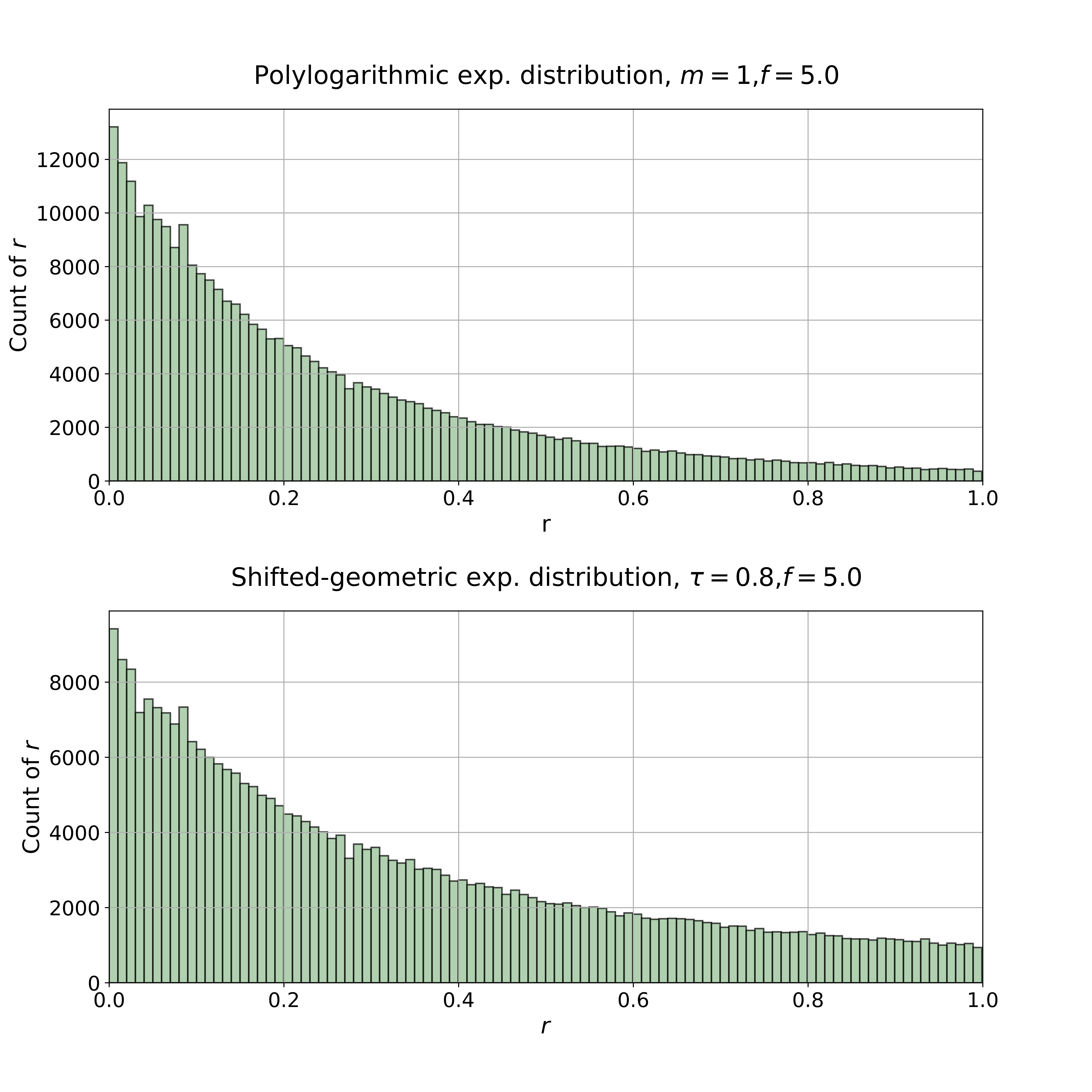
Figure 5: Histogram of 300,000 samples drawn from the polylogarithmic exponential distribution (Top) and from the shifted-geometric exponential distribution (Bottom).

4 Entropy-dominated homogeneous population

In the previous section, we introduced the widespread distribution using the base measure function in Eq. (1) $h\left(\mathbf{x}\right)$ given by Eq. (33). For the homogeneous population, this function cancels out with the binomial term, which includes the entropy term. In this section, we show that the condition $h\left(\mathbf{x}\right)=1$ (used in the standard homogeneous pairwise MaxEnt model) fails the cancellation of the entropy, which results in a concentrated distribution.

We now analyze the behaviour of the homogeneous PMF (Eq. (25)) with $h\left(Nr_{N}\right)=1$ as the number of neurons $N$ grows to infinity, while keeping the order of the polynomial part $Q_{N}\left(r_{N};\boldsymbol{\theta}_{N}\right)$ constant in $N$, i.e.,

$$\mathcal{O}\left(Q_{N}\left(r_{N};\boldsymbol{\theta}_{N}\right)\right)=\mathcal{O}\left(1\right).$$ (78)

Coupled with the Stirling formula for factorials using the order notation, i.e.,

$$N!=\sqrt{2\pi N}\left(\frac{N}{e}\right)^{N}\left(1+\mathcal{O}\left(\frac{1}{N}\right)\right),$$ (79)

the function $G_{N}\left(\cdot;\boldsymbol{\theta}_{N}\right)$ from the PMF (Eq. (25)) for $r_{N}\neq 0$ and $r_{N}\neq 1$ becomes (see the D for the details)

$$G_{N}\left(r_{N};\boldsymbol{\theta}_{N}\right) =-\frac{1}{N}\log\sqrt{2\pi Nr_{N}\left(1-r_{N}\right)}+H\left(r_{N}\right)+\frac{1}{N}Q_{N}\left(r_{N};\boldsymbol{\theta}_{N}\right)+\frac{1}{N}\mathcal{O}\left(\frac{1}{N}\right)$$

where $H\left(r_{N}\right)$ is the entropy term, defined as

$$H\left(r_{N}\right)=-r_{N}\log\left(r_{N}\right)-\left(1-r_{N}\right)\log\left(1-r_{N}\right).$$ (81)

Because the entropy order $\mathcal{O}\left(H\left(r_{N}\right)\right)=\mathcal{O}\left(1\right)$ is constant and considering Eq. (78), then the order of the function $NG_{N}\left(r_{N};\boldsymbol{\theta}_{N}\right)$ is

$$\mathcal{O} \left(-\log\sqrt{2\pi Nr_{N}\left(1-r_{N}\right)}+NH\left(r_{N}\right)+Q_{N}\left(r_{N};\boldsymbol{\theta}_{N}\right)+\mathcal{O}\left(\frac{1}{N}\right)\right)$$

$$=\mathcal{O}\left(-\sqrt{N}+N+1+\frac{1}{N}\right)$$

$$=\mathcal{O}\left(N\right).$$ (82)

Eq. (82) is the linear order of $N$ because the entropy term dominates over the other terms for large $N$.

The dominance of the entropy as $N\to\infty$ leads to the following delta PDF

$$\lim_{N\rightarrow\infty}\mathcal{P}\left(r_{N}|\boldsymbol{\theta}_{N}\right) =p\left(r|r^{*}\right)dr$$

$$=\delta\left(r-r^{*}\right)dr,$$ (83)

whose peak is concentrated at its maximum $r^{*}$ in the region dominated by the entropy. The corresponding distribution function is

$$\lim_{N\rightarrow\infty}F\left(r_{m}|r^{*}\right)= \int_{0}^{r_{m}}\delta\left(r-r^{*}\right)dr$$

$$= u\left(r_{m}-r^{*}\right),$$ (84)

where $u\left(\cdot\right)$ denotes the heavyside step function. For a proof of equations (83) and (84) see the D.

The result above indicates that with $h\left(\mathbf{x}\right)=1$ the distribution concentrates without canceling the entropy, unlike $h\left(\mathbf{x}\right)$ given by Eq. (19). Different base measure functions in the exponential family for the binary patterns correspond to different base measure functions of the homogeneous population models (either discrete or continuous). We summarize these correspondences in Table 1. Note that the base measure function of the homogeneous continuous population rate model approaches to the delta function if we use $h\left(\mathbf{x}\right)=1$. In this case, the limiting PDF is written by this base measure function alone (83).

We also note that most existing models, e.g., the K-pairwise maximum entropy model by Tkacik et al. [11, 21] and the DG model [26], do not explicitly define a base measure function for the binary patterns. According to our theory, when the discrete homogeneous distributions exhibit the widespread property (in the continuous limit), their corresponding function, $h\left(Nr_{N}\right)$, must contain an equivalent component that cancels with the entropy.

Table 1: The base measure functions of the population rate models for two choices of the $h\left(\cdot\right)$ function.

The base measure function $h\left(\mathbf{x}\right)$ of binary patterns distr. (Eq. 1)	Eq. (33)	$h\left(\mathbf{x}\right)=1$
The base measure function of homogeneous discrete pop. rate ($r_{N}$, Eq. (19))	1	$\sqrt{2\pi r_{N}\left(1-r_{N}\right)}\exp\left[NH\left(r_{N}\right)\right]$
The base measure function of homogeneous continuous pop. rate ($r$)	1	$\delta\left(r-r^{*}\right)$

Alternatively, we may consider that the models with widespread distributions are realized at a tuned parameter if we introduce a parameter that weights such function. The authors in [31] analyzed the homogeneous DG model by introducing a non-canonical parameter $\beta$ that scales the pattern distribution as $\mathcal{P}_{\beta}\left(\mathbf{x}|\boldsymbol{\theta}_{N}\right)=\mathcal{P}\left(\mathbf{x}|\boldsymbol{\theta}_{N}\right)^{\beta}/Z_{\beta}$, which sets an imbalance between the entropy term $H\left(r_{N}\right)$ and the one that comes from $h\left(Nr_{N}\right)^{\beta}$. The widespread distribution is only possible at $\beta=1$ in the limit of $N$, and they reported it as a phase transition along the parameter.

5 Discussion

We proposed parametric models of distributions for the sparse collective activity of homogeneous binary neurons. Our models exhibit HOIs at all orders in a way that agrees with structured alternating HOIs observed experimentally. The distribution remains widespread with parameter-dependent sparsity in the limit of an infinite number of neurons. We derived these models using a theoretical framework giving sufficient conditions by which the PMF of our binary population model, or any other homogeneous exponential family population rate model, converges to a widespread continuous distribution. Note that we obtained an exponential distribution with a bounded support in the limit of the large number of homogeneous independent neurons. While the independence resulted in the simplest sparse homogeneous model, observed interactions among the neurons further shape their population beyond the exponential distribution.

The proposed models explain how a sparse, widespread distribution arises from specific HOIs with alternating shrinking structure. Such models are expected to explain a sparse profile in spike-count population histograms of experimentally observed neurons [15, 10, 25, 21]. The models are also consistent with a previous theoretical prediction by [26], which states that all orders of interactions are required to produce a widespread activity distribution in a large population of (correlated) neurons. Here, we extended the theoretical framework in [26], showing that the base measure function, independently of the order of the (canonical) interactions, must be chosen carefully to avoid the dominance of the entropy term in the homogeneous distribution.

Although the sparse widespread distributions are ubiquitously observed in neural systems, the underlying mechanisms remain open to exploration. One of the simplest yet insightful models that can reproduce these key features is the dichotomized Gaussian (DG) model [26, 13] and its extentensions [32, 33, 34, 35], which consists of threshold-neurons that become active if inputs sampled from a correlated multivariate Gaussian distribution exceed a threshold. The outputs of the DG neurons, represented as $(0,1)$ patterns, exhibit sparse population activity [31, 16] with characteristic HOIs. Specifically, they display alternating signs in the interactions at successive orders, such as negative triplewise and positive quadruple-wise interactions and so on [16, 35]. The structured HOIs contribute to the sparse activity, and create the widespread distribution [26]. Supporting this theoretical prediction, the specific alternating structure of HOIs was found in neural population activity [16]. Furthermore, by using more biologically plausible model neurons, it was discovered in [17] that the positive pairwise and negative triple-wise interactions are explained by excitatory shared (and hence correlated) inputs to pairs of neurons. These results suggest that the nonlinearity of neurons underlie the structured HOIs, and investigating the HOIs of neuronal activity provides a key to understanding its underlying mechanisms.

The nonlinear functions to which the alternating shrinking series converge are key features of our models because they underlie HOIs and modulate the sparse population profile. We exemplified this by converging alternating series of the population rate using a logarithmic function and a function based on shifted-geometric series, which are both strictly decreasing functions of the population rate. The nonlinearity resulting in the HOIs of neurons come not only from spiking nonlinearity at the soma but also from the nonlinear operations at the dendrites. Examples of dendritic computation include directional selectivity, coincidence detection in auditory neurons, temporal integration, image denoising, forward masking [36] and nonlinear integration of spatial cortical feedback in V1 neurons [37]. As a support of the specific logarithmic operation, a modeling study of a collision-sensitive locust neuron, which considers experimentally determined presynaptic activation patterns, suggests that a single neuron’s dendritic tree implements a logarithmic transform [38]. Specifically, the fan-like dendritic structures in such neurons [39] have been suggested to support such nonlinear computations. It is thus a future challenge to construct a unifying model based on our framework for generating the sparse and widespread distribution such that the models account for the HOIs in neurons from more detailed mechanistic generation of sparse neural population activity.

6 Acknowledgements

We thank Miguel Aguilera for his valuable comments on this manuscript. This work was supported by JSPS KAKENHI Grant Number JP 20K11709, 21H05246.

Appendix A Homogeneous sparse population of neurons

A.1 Proof of Theorem 1

In the limit as $N\to\infty$ the homogeneous population rate distribution will become concentrated at $r^{0}_{N}$ if it converges to a delta peak at that location. For the PMF (25) to become a non-concentrated or widespread distribution, it must hold [26]

$$\lim_{N\to\infty}N\left[G_{N}\left(r_{N};\boldsymbol{\theta}_{N}\right)-G_{N}\left(r^{0}_{N};\boldsymbol{\theta}_{N}\right)\right]<\infty$$ (85)

$$\forall\;r^{0}_{N}\neq r_{N}\;\in S_{r}.$$

Because of the constant order of $NG_{N}\left(r_{N};\boldsymbol{\theta}_{N}\right)$ (see Eq. (30)) we have

$$\mathcal{O}\left(NG_{N}\left(r_{N};\boldsymbol{\theta}_{N}\right)-NG_{N}\left(r^{0}_{N};\boldsymbol{\theta}_{N}\right)\right)=\mathcal{O}\left(1\right)$$ (86)

and hence inequality (85) holds for $G_{N}\left(r_{N};\boldsymbol{\theta}_{N}\right)<\infty$ with $r_{N}\in S_{r}$. This proves that (25) becomes widespread in the limit of $N\to\infty$.

On the other hand, recall $G_{N}\left(\cdot\right)$ is a non-positive strictly decreasing function with finite values in $S_{r}$. This means the maximum value for $G_{N}\left(r_{N};\boldsymbol{\theta}_{N}\right)$ and also for the PMF (25) will be at $\inf\left\{S_{r}\right\}=\inf\left\{0,\frac{1}{N},\frac{2}{N},\ldots,1\right\}=0$. Further, the maximum remains at $0$ in the limit $\lim_{N\to\infty}\mathcal{P}\left(r_{N}|\boldsymbol{\theta}_{N}\right)=p\left(r|\boldsymbol{\lambda}\right)dr$ since $S_{r}\to[0,1]$ as $N\to\infty$ and by continuity of the strictly decreasing property of $G_{N}\left(\cdot\right)$.

A.2 Independent homogeneous model

The distribution function corresponding to the PDF from Eq. (38) is

$$F\left(u|f\right) =\frac{1-e^{-\mathpzc{f}u}}{1-e^{-\mathpzc{f}}}.$$ (87)

The mean is given by

$$\mu_{R} =\frac{1}{Z}\int_{0}^{1}e^{-\mathpzc{f}r}rdr=\frac{1}{\mathpzc{f}\left(1-e^{-\mathpzc{f}}\right)}-\frac{e^{-\mathpzc{f}}}{1-e^{-\mathpzc{f}}}\left(1+\frac{1}{\mathpzc{f}}\right),$$ (88)

and the variance is

$$\sigma_{R}^{2} =\frac{1}{Z}\int_{0}^{1}e^{-\mathpzc{f}r}r^{2}dr-\mu_{R}^{2}$$

$$=\frac{2}{\mathpzc{f}^{2}\left(1-e^{-\mathpzc{f}}\right)}-\frac{e^{-\mathpzc{f}}}{1-e^{-\mathpzc{f}}}\left(\frac{2}{\mathpzc{f}^{2}}+\frac{2}{\mathpzc{f}}\right)-\frac{1}{\mathpzc{f}}e^{-\mathpzc{f}}-\mu_{R}^{2}.$$ (89)

Appendix B The model with alternating and shrinking higher-order interactions

B.1 Canonical coordinates

The sum of total binary activity elevated to a given power $k>0$ and $k\leq N$ can be expanded as follows (using the Multinomial Theorem)

$$\left(\sum_{i=1}^{N}x_{i}\right)^{k}= \sum_{i=1}^{N}x_{i}^{k}+\sum_{i_{1}<i_{2}}\sum_{\begin{subarray}{c}k_{i_{1}}+k_{i_{2}}=k\\ \end{subarray}}\left(\begin{array}[]{c}k\\ k_{i_{1}},k_{i_{2}}\end{array}\right)x_{i_{1}}^{k_{i_{1}}}x_{i_{2}}^{k_{i_{2}}}$$ (92)

$$+\sum_{i_{1}<i_{2}<i_{3}}\sum_{\begin{subarray}{c}k_{i_{1}}+k_{i_{2}}+k_{i_{3}}=k\\ \end{subarray}}\left(\begin{array}[]{c}k\\ k_{i_{1}},k_{i_{2}},k_{i_{3}}\end{array}\right)x_{i_{1}}^{k_{i_{1}}}x_{i_{2}}^{k_{i_{2}}}x_{i_{3}}^{k_{i_{3}}}$$ (95)

$$+\cdots+\sum_{i_{1}<i_{2}<\ldots<i_{k}}k!\,x_{i_{1}}x_{i_{2}}\ldots x_{i_{k}},$$ (96)

where $\left(\begin{array}[]{c}k\\ k_{i_{1}},k_{i_{2}},\ldots,k_{N}\end{array}\right)=\frac{k!}{k_{i_{1}}!k_{i_{2}}!\cdots k_{i_{N}}!}$ is a multinomial coefficient with $k_{i_{1}}>0,k_{i_{2}}>0,\ldots,k_{{}_{i_{N}}}>0$. Using the fact that any $x_{i}$ is binary, the powers of $x_{i}$ in Eq. (96) reduce as follows

$$\left(\sum_{i=1}^{N}x_{i}\right)^{k}= \sum_{i=1}^{N}x_{i}+\sum_{i_{1}<i_{2}}\sum_{\begin{subarray}{c}k_{i_{1}}+k_{i_{2}}=k\\ \end{subarray}}\left(\begin{array}[]{c}k\\ k_{i_{1}},k_{i_{2}}\end{array}\right)x_{i_{1}}x_{i_{2}}+\cdots+$$ (99)

$$+\sum_{i_{1}<i_{2}<i_{3}}\sum_{\begin{subarray}{c}k_{i_{1}}+k_{i_{2}}+k_{i_{3}}=k\\ \end{subarray}}\left(\begin{array}[]{c}k\\ k_{i_{1}},k_{i_{2}},k_{i_{3}}\end{array}\right)x_{i_{1}}x_{i_{2}}x_{i_{3}}$$ (102)

$$+\cdots+\sum_{i_{1}<i_{2}<\ldots<i_{k}}k!\,x_{i_{1}}x_{i_{2}}\ldots x_{i_{k}}.$$ (103)

Following the multinomial expansion from Eq. (103) the canonical form of our binary PMF can be obtained as follows

$$\mathcal{P}\left(\mathbf{x}|\boldsymbol{\omega}\right) =\frac{h\left(\mathbf{x}\right)}{Z}\exp\left[-\mathpzc{f}\sum\limits_{j=1}^{N}\left(-1\right)^{j+1}C_{j}\left(\frac{\sum_{i=1}^{N}x_{i}}{N}\right)^{j}\right]$$

$$=\frac{h\left(\mathbf{x}\right)}{Z}\exp\left[-\mathpzc{f}\left(C_{1}\frac{\sum_{i=1}^{N}x_{i}}{N}-C_{2}\frac{\left(\sum_{i=1}^{N}x_{i}\right)^{2}}{N^{2}}\right.\right.$$

$$\;\;\;\;\;\;\;\;\;\;\;\;\;\;\;\;\;\;\;\;\;\;\;\;\;\;\;\;\;\;\left.\left.+\ldots+\left(-1\right)^{N+1}C_{N}\frac{\left(\sum_{i=1}^{N}x_{i}\right)^{N}}{N^{N}}\right)\right]$$

$$=\frac{h\left(\mathbf{x}\right)}{Z}\exp\left[-\frac{\mathpzc{f}C_{1}}{N}\sum\limits_{i=1}^{N}x_{i}\right.$$

$$\phantom{\frac{h\left(\mathbf{x}\right)}{Z}\exp=}+\frac{\mathpzc{f}C_{2}}{N^{2}}\left(\sum\limits_{i=1}^{N}x_{i}\right)^{2}$$

$$\phantom{\frac{h\left(\mathbf{x}\right)}{Z}\exp=}-\frac{\mathpzc{f}C_{3}}{N^{3}}\left(\sum\limits_{i=1}^{N}x_{i}\right)^{3}$$

$$\phantom{\frac{h\left(\mathbf{x}\right)}{Z}\exp==}\vdots$$

$$\phantom{\frac{h\left(\mathbf{x}\right)}{Z}\exp=}\left.+\left(-1\right)^{N+1}\frac{\mathpzc{f}C_{N}}{N^{N}}\left(\sum\limits_{i=1}^{N}x_{i}\right)^{N}\right]$$

$$=\frac{h\left(\mathbf{x}\right)}{Z}\exp\left[-\frac{\mathpzc{f}C_{1}}{N}\sum\limits_{i=1}^{N}x_{i}\right.$$

$$\phantom{\frac{h\left(\mathbf{x}\right)}{Z}\exp=}+\frac{\mathpzc{f}C_{2}}{N^{2}}\left(\sum_{i=1}^{N}x_{i}+2\sum_{i_{1}<i_{2}}x_{i_{1}}x_{i_{2}}\right)$$

$$\phantom{\frac{h\left(\mathbf{x}\right)}{Z}\exp=}-\frac{\mathpzc{f}C_{3}}{N^{3}}\left(\sum_{i=1}^{N}x_{i}+6\sum_{i_{1}<i_{2}}x_{i_{1}}x_{i_{2}}+6\sum_{i_{1}<i_{2}<i_{3}}x_{i_{1}}x_{i_{2}}x_{i_{3}}\right)$$

$$\phantom{\frac{h\left(\mathbf{x}\right)}{Z}\exp==}\vdots$$

$$\phantom{\frac{h\left(\mathbf{x}\right)}{Z}\exp=}+\left.\left(-1\right)^{N+1}\frac{\mathpzc{f}C_{N}}{N^{N}}\left(\sum\limits_{i=1}^{N}x_{i}+\sum_{i_{1}<i_{2}}\sum_{\begin{subarray}{c}k_{1}+k_{2}=N\end{subarray}}\left(\begin{array}[]{c}N\\ k_{1},k_{2}\end{array}\right)x_{i_{1}}x_{i_{2}}\right.\right.$$ (106)

$$\;\;\;\;\;\;\;\;\;\;\;\;\;\;\;\;\;\;\;\;\;\;\;\;\;\;\;\;\;\;\;\;\;\;\;\;\;\;\;\;\;\;\;\;\;\;\;\;\;\;\;\;\;\;\;\;\;\;\;\;\;\;\;\;\;+\ldots+N!\,x_{i_{1}}x_{i_{2}}\ldots x_{i_{N}}\Bigg{)}\Bigg{]}$$

Here we compare the above equation with the canonical form of the exponential family distribution:

$$\mathcal{P}\left(\mathbf{x}|\boldsymbol{\theta}_{N}\right)=\frac{h\left(\mathbf{x}\right)}{Z}\exp\left[\theta_{1}\sum\limits_{i=1}^{N}x_{i}+\theta_{2}\sum_{i_{1}<i_{2}}x_{i_{1}}x_{i_{2}}+\ldots+\theta_{N}x_{i_{1}}x_{i_{2}}\ldots x_{i_{N}}\right],$$ (108)

where $h\left(\mathbf{x}\right)$ is defined as in Eq. (33). The canonical parameter $\boldsymbol{\theta}_{N}$ is obtained by grouping the coefficients that multiply every power function of the coordinates in $\mathbf{x}$, i.e.,

$$\theta_{1}= \sum_{l=1}^{N}\left(-1\right)^{l}\frac{\mathpzc{f}C_{l}}{N^{l}},$$

$$\theta_{2}= \sum_{l=2}^{N}\left(-1\right)^{l}\frac{\mathpzc{f}C_{l}}{N^{l}}\sum\limits_{\begin{subarray}{c}k_{1}+k_{2}=l\end{subarray}}\left(\begin{array}[]{c}l\\ k_{1},k_{2}\end{array}\right),$$ (111)

$$\vdots$$

$$\theta_{N}= \left(-1\right)^{N}\frac{\mathpzc{f}C_{N}}{N^{N}}N!.$$ (112)

B.2 Population rate probability density function

We now show the proof to obtain our limiting alternating PDF from Eq. (50). For the remainder of the homogeneous analysis we make use of Stirling numbers of the first kind, which are defined as follows for $m>0$

$$s\left(k,m\right)=\left(-1\right)^{k-m}\left[\begin{array}[]{c}k\\ m\end{array}\right],$$ (115)

where

$$\left[\begin{array}[]{c}k\\ m\end{array}\right]=\left(k-1\right)\left[\begin{array}[]{c}k-1\\ m\end{array}\right]+\left[\begin{array}[]{c}k-1\\ m-1\end{array}\right],$$ (122)

with the initial conditions (for $k>0$)

$$\left[\begin{array}[]{c}0\\ 0\end{array}\right]=1,\;\;\;\;\;\left[\begin{array}[]{c}k\\ 0\end{array}\right]=\left[\begin{array}[]{c}0\\ k\end{array}\right]=0,$$ (129)

and the identity

$$\left[\begin{array}[]{c}k\\ k\end{array}\right]=1.$$ (132)

Stirling numbers of the first kind are useful to rewrite the binomial coefficients in an expanded polynomial form as follows

$$\left(\begin{array}[]{c}n\\ k\end{array}\right)=\frac{1}{k!}\sum_{m=0}^{k}s\left(k,m\right)n^{m}.$$ (133)

The polynomial term in the exponential argument of our alternating PMF is

$$Q_{N}\left(r_{N};\boldsymbol{\theta}_{N}\right) =\sum\limits_{k=1}^{Nr_{N}}\left(\begin{array}[]{c}Nr_{N}\\ k\end{array}\right)\theta_{k}$$ (136)

$$=\sum\limits_{k=1}^{Nr_{N}}\frac{1}{k!}\sum\limits_{m=0}^{k}s\left(k,m\right)\left(Nr_{N}\right)^{m}\theta_{k}$$

$$=\sum\limits_{k=1}^{Nr_{N}}\theta_{k}\sum\limits_{m=0}^{k}\left(-1\right)^{k-m}\left[\begin{array}[]{c}k\\ m\end{array}\right]\frac{\left(Nr_{N}\right)^{m}}{k!}$$ (139)

$$=\sum\limits_{k=1}^{Nr_{N}}\theta_{k}\left[\left(-1\right)^{k}\left[\begin{array}[]{c}k\\ 0\end{array}\right]\frac{\left(Nr_{N}\right)^{0}}{k!}+\left(-1\right)^{0}\left[\begin{array}[]{c}k\\ k\end{array}\right]\frac{\left(Nr_{N}\right)^{k}}{k!}+\right.$$ (144)

$$\phantom{======}\left.\sum\limits_{m=1}^{k-1}\left(-1\right)^{k-m}\left[\begin{array}[]{c}k\\ m\end{array}\right]\frac{\left(Nr_{N}\right)^{m}}{k!}\right]$$ (147)

$$=\sum\limits_{k=1}^{Nr_{N}}\theta_{k}\left[\frac{\left(Nr_{N}\right)^{k}}{k!}\right]+\sum\limits_{k=1}^{Nr_{N}}\theta_{k}\left[\sum\limits_{m=1}^{k-1}\left(-1\right)^{k-m}\left[\begin{array}[]{c}k\\ m\end{array}\right]\frac{\left(Nr_{N}\right)^{m}}{k!}\right],$$ (150)

where the later was obtained using the identities (129) and (132). The first term in the last right hand side of Eq. (150) can be expanded as

$$\sum\limits_{k=1}^{Nr_{N}}\theta_{k}\left[\frac{\left(Nr_{N}\right)^{k}}{k!}\right] =\sum\limits_{l=1}^{N}\left(-1\right)^{l}\mathpzc{f}\frac{C_{l}}{N^{l}}\left(Nr_{N}\right)$$

$$\;\;\;\;\;+\sum\limits_{l=2}^{N}\left(-1\right)^{l}\mathpzc{f}\frac{C_{l}}{N^{l}}\sum\limits_{\begin{subarray}{c}k_{1}+k_{2}=l\end{subarray}}\left(\begin{array}[]{c}l\\ k_{1},k_{2}\end{array}\right)\frac{\left(Nr_{N}\right)^{2}}{2!}$$ (153)

$$\;\;\;\;\;+\ldots$$

$$\;\;\;\;\;+\sum\limits_{l=Nr_{N}}^{N}\left(-1\right)^{l}\mathpzc{f}\frac{C_{l}}{N^{l}}\sum\limits_{\begin{subarray}{c}k_{1}+\ldots+k_{Nr_{N}}=l\end{subarray}}\left(\begin{array}[]{c}l\\ k_{1},\ldots,k_{Nr_{N}}\end{array}\right)\frac{\left(Nr_{N}\right)^{Nr_{N}}}{\left(Nr_{N}\right)!}$$ (156)

$$=\left(-1\right)^{1}\mathpzc{f}\frac{C_{1}}{N^{1}}Nr_{N}+\sum\limits_{l=2}^{N}\left(-1\right)^{l}\mathpzc{f}\frac{C_{l}}{N^{l}}Nr_{N}$$

$$\;\;\;\;\;+\rule{0.0pt}{28.45274pt}\left(-1\right)^{2}\mathpzc{f}\frac{C_{2}2!}{N^{2}}\frac{N^{2}\left(r_{N}\right)^{2}}{2!}+\sum\limits_{l=3}^{N}\left(-1\right)^{l}\mathpzc{f}\frac{C_{l}}{N^{l}}\sum\limits_{\begin{subarray}{c}k_{1}+k_{2}=l\end{subarray}}\left(\begin{array}[]{c}l\\ k_{1},k_{2}\end{array}\right)\frac{\left(Nr_{N}\right)^{2}}{2!}$$ (159)

$$\;\;\;\;\;+\ldots$$

$$\;\;\;\;\;+\rule{0.0pt}{28.45274pt}\left(-1\right)^{Nr_{N}}\mathpzc{f}\frac{C_{Nr_{N}}\left(Nr_{N}\right)!}{N^{Nr_{N}}}\frac{N^{Nr_{N}}r^{Nr_{N}}}{\left(Nr_{N}\right)!}$$

$$\;\;\;\;\;\;\;\;\;\;\;\;\;+\sum\limits_{l=Nr_{N}+1}^{N}\left(-1\right)^{l}\mathpzc{f}\frac{C_{l}}{N^{l}}\sum\limits_{\begin{subarray}{c}k_{1}+\ldots+k_{Nr_{N}}=l\end{subarray}}\left(\begin{array}[]{c}l\\ k_{1},\ldots,k_{Nr_{N}}\end{array}\right)\frac{N^{Nr_{N}}\left(r_{N}\right)^{Nr_{N}}}{\left(Nr_{N}\right)!}$$ (162)

$$=\sum\limits_{j=1}^{Nr_{N}}\left(-1\right)^{j}\mathpzc{f}\frac{C_{j}}{N^{j}}N^{j}\left(r_{N}\right)^{j}+\mathcal{O}\left(\frac{1}{N}\right)$$

$$=\sum\limits_{j=1}^{Nr_{N}}\left(-1\right)^{j}\mathpzc{f}C_{j}\left(r_{N}\right)^{j}+\mathcal{O}\left(\frac{1}{N}\right)$$

$$=-\mathpzc{f}\sum\limits_{j=1}^{Nr_{N}}\left(-1\right)^{j+1}C_{j}\left(r_{N}\right)^{j}+\mathcal{O}\left(\frac{1}{N}\right).$$ (163)

On the other hand, we can obtain the order for the second term in the last right hand side of Eq. (150) as follows

$$\mathcal{O}\left(\sum\limits_{k=1}^{Nr_{N}}\theta_{k}\left[\sum\limits_{m=1}^{k-1}\left(-1\right)^{k-m}\left[\begin{array}[]{c}k\\ m\end{array}\right]\frac{N^{m}\left(r_{N}\right)^{m}}{k!}\right]\right)$$ (166)

$$=\mathcal{O}\left(\theta_{1}+\theta_{2}\left(-1\right)\left[\begin{array}[]{c}2\\ 1\end{array}\right]\frac{N^{1}\left(r_{N}\right)^{1}}{2!}+\right.$$ (169)

$$\;\;\;\;\;\;\;\;\;\;\left.+\ldots+\theta_{Nr_{N}}\sum\limits_{m=1}^{Nr_{N}-1}\left(-1\right)^{Nr_{N}-m}\left[\begin{array}[]{c}Nr_{N}\\ m\end{array}\right]\frac{N^{m}\left(r_{N}\right)^{m}}{\left(Nr_{N}\right)!}\right),$$ (172)

where the highest order for each $\theta_{k}$ corresponds to its first term (since its terms grow inversely in $N$). The order is then

$$\mathcal{O}\left(\sum\limits_{k=1}^{Nr_{N}}\theta_{k}\left[\sum\limits_{m=1}^{k-1}\left(-1\right)^{k-m}\left[\begin{array}[]{c}k\\ m\end{array}\right]\frac{N^{m}\left(r_{N}\right)^{m}}{k!}\right]\right)$$ (175)

$$=\mathcal{O}\left(\frac{1}{N}+\frac{1}{N^{2}}2!\frac{N}{2!}+\ldots+\frac{1}{N^{Nr_{N}}}\left(Nr_{N}\right)!\frac{N^{Nr_{N}-1}}{\left(Nr_{N}\right)!}\right)$$

$$=\mathcal{O}\left(\frac{1}{N}\right).$$ (176)

Considering Eqs. (150), (163) and (176), the polynomial term can be written as in Eq. (49) and our PMF becomes

$$\mathcal{P}\left(r_{N}|\boldsymbol{\theta}_{N}\right) =\frac{1}{Z}\exp\left[-\mathpzc{f}\sum\limits_{j=1}^{Nr_{N}}\left(-1\right)^{j+1}C_{j}\left(r_{N}\right)^{j}+\mathcal{O}\left(\frac{1}{N}\right)\right].$$ (177)

B.3 Widespread probability density function limit

Using Eq. (177) in the limit as $N\to\infty$ our PMF becomes

$$\lim_{N\rightarrow\infty}\mathcal{P}\left(r_{N}|\boldsymbol{\theta}_{N}\right) =\frac{1}{Z}\exp\left[-\mathpzc{f}\sum\limits_{j=1}^{\infty}\left(-1\right)^{j+1}C_{j}r^{j}\right]dr$$

$$=p\left(r|\boldsymbol{\lambda}\right)dr,$$ (178)

where $\boldsymbol{\lambda}=\left\{\mathpzc{f},\left\{C_{j}\right\}_{j\in\mathbb{N}^{+}}\right\}$. The specific form of the distribution (178) and its convergence depends on the $C_{j}$ constants. By Leibniz criterion for alternating series the following series in our alternating density

$$-\mathpzc{f}\sum_{j=1}^{\infty}\left(-1\right)^{j+1}C_{j}r^{j}= \mathpzc{f}\sum_{j=1}^{\infty}\left(-1\right)^{j}C_{j}r^{j}$$ (179)

converge if the following conditions hold:

$$|C_{1}r|>|C_{2}r^{2}|>|C_{3}r^{3}|>\ldots,$$

$$\lim\limits_{j\to\infty}\left[C_{j}r^{j}\right]=0.$$ (180)

The conditions in Eq. (180) hold for the following cases, but are not restricted to them.

Polylogarithmic exponential PDF

If we define $C_{j}=\frac{1}{j^{m}}\;\;\forall j\;\;$ then the PDF in (178) is as in Eq. (51), where $\text{Li}_{m}[\cdot]$ is the polylogarithm function of order $m=1,2,3,\ldots$, defined as

$$\text{Li}_{m}\left[x\right]=\sum_{j=1}^{\infty}\frac{x^{j}}{j^{m}}$$ (181)

When $m=1$ the series converge to the natural logarithm, i.e., Eq. (52).

Shifted-geometric exponential PDF

If we instead define $C_{j}=\left(\tau\right)^{j}$, with $\;0<\tau<1,\;\forall j\;\;$ so that $\tau r<1$ then the distribution in (178) is as in Eq. (66). To see why Eq. (66) holds, we consider the following

$$\lim\limits_{n\to\infty}\left[-\mathpzc{f}\sum_{j=1}^{n}\left(-1\right)^{j+1}\left(\tau r\right)^{j}\right]= \mathpzc{f}\lim\limits_{n\to\infty}\left[\sum_{j=1}^{n}\left(-1\right)^{j}\left(\tau r\right)^{j}\right]$$

$$= \mathpzc{f}\lim\limits_{n\to\infty}\left[\sum_{j=1}^{n}\left(-\tau r\right)^{j}\right]$$

$$= \mathpzc{f}\lim\limits_{n\to\infty}\left[\frac{-\left(\tau r+\left(-1\right)^{n+1}\left(\tau r\right)^{n+1}\right)}{1+\tau r}\right]$$

$$= -\mathpzc{f}\frac{1}{1+\frac{1}{\tau r}}$$

$$= \mathpzc{f}\left(\frac{1}{1+\tau r}-1\right).$$ (182)

Appendix C Properties of the polylogarithmic and Shifted-geometric exponential densities

C.1 Non-positive property for the arguments of the exponential function

Polylogarithmic exponential density

For $m=1$ we have the function

$$\mathpzc{f}\text{Li}_{1}\left[-r\right]=-\mathpzc{f}\log\left(1+r\right)\leq 0\phantom{==}\forall r\in[0,1]$$ (183)

because $\log\left(x\right)$ is a strictly increasing function for $x>0$ and correspondingly $-\mathpzc{f}\log\left(x\right)$ ($\mathpzc{f}>0$) is a strictly decreasing function for $x>0$, where $-\mathpzc{f}\log\left(1+r\right)=0$ for $r=0$ and $-\mathpzc{f}\log\left(1+r\right)=-\mathpzc{f}\log 2$ for $r=1$. Then inequality (183) holds for $r\in[0,1]$ and $-\mathpzc{f}\log\left(1+r\right)$ has a maximum at $r=0$.

For $m\in\left\{2,3,4,\ldots\right\}$ the following alternating series (shown on the right hand side in parenthesis)

$$\mathpzc{f}\text{Li}_{m}\left[-r\right]=\mathpzc{f}\left(\sum\limits_{j=1}^{\infty}\frac{\left(-r\right)^{j}}{j^{m}}\right)$$ (184)

converge to a finite limit $L$ by the Leibniz criterion. In this case $L=\text{Li}_{m}\left[-r\right]$, and the convergence proof of Leibniz criterion for alternating series guarantees the following bounds for any $n>0$

$$S_{2n}\leq L\leq S_{2n+1},$$ (185)

where $S_{2n}$ denotes the partial sum of an even number of terms and $S_{2n+1}$ denotes the partial sum of an odd number of terms in the alternating series. Then we have the partial sum with an even number of terms ($2n=2$)

$$S_{2} =\sum\limits_{j=1}^{2}\frac{\left(-r\right)^{j}}{j^{m}}$$

$$=-r+\frac{r^{2}}{2^{m}}\leq 0\phantom{==}\forall r\in[0,1],$$ (186)

where the last inequality holds because the coefficient of the first negative term is such that $r\geq r^{2}\geq\frac{r^{2}}{2^{m}}\phantom{==}\forall r\in[0,1]$. Similarly we have the following partial sum with an odd number of terms ($2n+1=3$)

$$S_{3} =\sum\limits_{j=1}^{3}\frac{\left(-r\right)^{j}}{j^{m}}$$

$$=S_{2}-\frac{r^{3}}{3^{m}}\leq 0\phantom{==}\forall r\in[0,1],$$ (187)

where the last inequality holds because $S_{2}\leq 0$ by inequality (186) and since $-\frac{r^{3}}{3^{m}}\leq 0$ for $r\in[0,1]$. Using inequalities (185) and (187) we have for $m\in\left\{2,3,4,\ldots\right\}$ that

$$\text{Li}_{m}\left[-r\right]\leq 0\phantom{==}\forall r\in[0,1]$$ (188)

and also for $\mathpzc{f}>0$ we have $\mathpzc{f}\text{Li}_{m}\left[-r\right]\leq 0$ . Consequently by Eqs. (188) and (183) the function in Eq. (184) is non-positive for $r\in[0,1]$ with $m\in\left\{1,2,3,\ldots\right\}$.

Shifted-geometric exponential density

For the shifted-geometric function we have the following inequality

$$\mathpzc{f}\left(\frac{1}{1+\tau r}-1\right)\leq 0\phantom{==}\forall r\in[0,1]$$ (189)

because for $\tau>0$ it holds that $\frac{1}{1+\tau r}\leq 1$ for $r\in[0,1]$. Equality in Eq. (189) is reached only when $r=0$ and hence $\mathpzc{f}\left(\frac{1}{1+\tau r}-1\right)$ is non-positive with a maximum at $r=0$.

C.2 Decreasing property for the arguments of the exponential function

Polylogarithmic exponential density
We now prove the decreasing property for the polylogarithmic function in the polylogarithmic exponential density in Eq. (51). For $m=1$ the derivative of the function is

$$\frac{d}{dr}\left[\mathpzc{f}\text{Li}_{1}\left[-r\right]\right] =\frac{d}{dr}\left[-\mathpzc{f}\log\left(1+r\right)\right]$$

$$=-\frac{\mathpzc{f}}{1+r}<0\phantom{==}\forall r\in[0,1],$$ (190)

since $\mathpzc{f}>0$. On the other hand, for $m\in\left\{2,3,4,\ldots\right\}$ the derivative is

$$\frac{d}{dr}\left[\mathpzc{f}\text{Li}_{m}\left[-r\right]\right] =\mathpzc{f}\frac{d}{dr}\left[\text{Li}_{m}\left[-r\right]\right]$$

$$=\mathpzc{f}\left[\frac{1}{r}\text{Li}_{m-1}\left[-r\right]\right]$$

$$=\mathpzc{f}\left[\sum\limits_{j=1}^{\infty}\left(-1\right)^{j}\left(\frac{r^{j-1}}{j^{m-1}}\right)\right],$$ (191)

where $\frac{r^{j-1}}{j^{m-1}}>\frac{r^{j}}{\left(j+1\right)^{m-1}}$ and $\lim_{j\to\infty}\left[\frac{r^{j-1}}{j^{m-1}}\right]=0$. Then, by the Leibniz criterion, the alternating series of $\frac{d}{dr}\left[\text{Li}_{m}\left[-r\right]\right]$ converge to a finite limit $L$. Using the bounds in Eq. (185) for $n=1$ it holds that

$$S_{2}\leq L\leq S_{3}.$$ (192)

The partial sum for the even number of terms is

$$S_{2} =-\frac{r^{0}}{1^{m-1}}+\frac{r^{1}}{2^{m-1}}$$

$$=-1+\frac{r}{2^{m-1}}<0\phantom{==}\forall r\in[0,1]$$ (193)

because $S_{2}$ increases linearly in $r$ but is always negative since we have at the extremes $S_{2}=-1$ when $r=0$ and $S_{2}=-1+\frac{1}{2^{m-1}}<0$ when $r=1$ for $m\in\left\{2,3,4,\ldots\right\}$. Similarly we have for the partial sum with odd number of terms

$$S_{3} =-1+\frac{r}{2^{m-1}}-\frac{r^{2}}{3^{m-1}}$$

$$=S_{2}-\frac{r^{2}}{3^{m-1}}<0$$ (194)

because $S_{2}<0$ and $-\frac{r^{2}}{3^{m-1}}<0\;\;\forall r\in[0,1],m\in\left\{2,3,4,\ldots\right\}$. Consequently we have that

$$\frac{d}{dr}\left[\mathpzc{f}\text{Li}_{m}\left[-r\right]\right] =\mathpzc{f}\frac{d}{dr}\left[\text{Li}_{m}\left[-r\right]\right]$$

$$=\mathpzc{f}L<0\phantom{==}\forall r\in[0,1],$$ (195)

with $m\in\left\{2,3,4,\ldots\right\}$. By inequalities (190) and (C.2) it holds that

$$\frac{d}{dr}\left[\mathpzc{f}\text{Li}_{m}\left[-r\right]\right]<0 \phantom{==}\forall r\in[0,1],$$ (196)

$$\phantom{==}m\in\left\{1,2,3,\ldots\right\},$$

and hence the function $\mathpzc{f}\text{Li}_{m}\left[-r\right]$ is strictly decreasing for $r\in[0,1]$ and $m\in\left\{1,2,3,\ldots\right\}$.

Shifted-geometric exponential density

Next we prove the decreasing property for the shifted-geometric function in the shifted-geometric exponential density in Eq. (66). The derivative of the function is

$$\frac{d}{dr}\left[\mathpzc{f}\left(\frac{1}{1+\tau r}-1\right)\right] =\mathpzc{f}\frac{d}{dr}\left[\left(\frac{1}{1+\tau r}-1\right)\right]$$

$$=\mathpzc{f}\frac{d}{dr}\left[\left(1+\tau r\right)^{-1}\right]$$

$$=-\frac{\mathpzc{f}\tau}{\left(1+\tau r\right)^{2}}<0\phantom{==}\forall r\in[0,1]$$ (197)

because $\mathpzc{f}>0$, $\tau>0$ and $\left(1+\tau r\right)^{2}>0$. It follows that the function $\mathpzc{f}\left(\frac{1}{1+\tau r}-1\right)$ is strictly decreasing for $r\in[0,1]$ and $0<\tau<1$.

C.3 Integrals for the shifted-geometric exponential distribution

We now verify the definite integral result from Eq. (67). Since $F\left(u|\mathpzc{f},\tau\right)$ denotes the distribution function evaluated at $u$ we have that

$$F\left(1|\mathpzc{f},\tau\right)=\frac{1}{Z}\int_{0}^{1}\exp\left[\mathpzc{f}\left(\frac{1}{1+\tau r}-1\right)\right]dr=1.$$ (198)

From Eq. (198) we obtain the normalization constant

$$Z =\int_{0}^{1}\exp\left[\mathpzc{f}\left(\frac{1}{1+\tau r}-1\right)\right]dr$$

$$=\left(\frac{1+\tau r}{\tau}\exp\left[\mathpzc{f}\left(\frac{1}{1+\tau r}-1\right)\right]-\frac{\mathpzc{f}e^{-\mathpzc{f}}}{\tau}\text{Ei}\left(\frac{\mathpzc{f}}{1+\tau r}\right)\right)\Bigg{|}_{0}^{1}.$$ (199)

The last right hand side of Eq. (199) contains the indefinite integral of $\exp\left[\mathpzc{f}\left(\frac{1}{1+\tau r}-1\right)\right]dr$ to be evaluated from $0$ to $1$. We now obtain the derivative of such indefinite integral. For this we make use of the series representation of the special exponential integral function $\text{Ei}\left(x\right)$ when its argument $x$ is real, defined in Eq. (68). The derivative is then

$$\frac{d}{dr}\left[\frac{1+\tau r}{\tau}\exp\left[\mathpzc{f}\left(\frac{1}{1+\tau r}-1\right)\right]-\frac{\mathpzc{f}e^{-\mathpzc{f}}}{\tau}\text{Ei}\left(\frac{\mathpzc{f}}{1+\tau r}\right)\right]$$

$$=\frac{d}{dr}\left[\frac{1+\tau r}{\tau}\exp\left[\mathpzc{f}\left(\frac{1}{1+\tau r}-1\right)\right]-\frac{\mathpzc{f}e^{-\mathpzc{f}}}{\tau}\left(\gamma+\log\left(\frac{\mathpzc{f}}{1+\tau r}\right)+\sum\limits_{k=1}^{\infty}\frac{\left(\frac{\mathpzc{f}}{1+\tau r}\right)^{k}}{k\;k!}\right)\right]$$

$$=\left(-\frac{\mathpzc{f}}{\left(1+\tau r\right)^{2}}+1-\tau r\frac{\mathpzc{f}}{\left(1+\tau r\right)^{2}}\right)\exp\left[\mathpzc{f}\left(\frac{1}{1+\tau r}-1\right)\right]+\phantom{================}$$

$$\phantom{==}\left(-\frac{\mathpzc{f}e^{-\mathpzc{f}}}{\tau}\left[-\frac{\tau\mathpzc{f}^{0}\left(1+\tau r\right)^{-1}}{0!}-\frac{\tau\mathpzc{f}^{1}\left(1+\tau r\right)^{-2}}{1!}-\frac{\tau\mathpzc{f}^{2}\left(1+\tau r\right)^{-3}}{2!}-\ldots\right]\right)$$

$$=\left(1-\left(\frac{\mathpzc{f}}{\left(1+\tau r\right)^{2}}\left(1+\tau r\right)\right)\right)\exp\left[\mathpzc{f}\left(\frac{1}{1+\tau r}-1\right)\right]+$$

$$\phantom{================}\left(\frac{\mathpzc{f}}{1+\tau r}\right)e^{-\mathpzc{f}}\sum\limits_{k=1}^{\infty}\frac{\left(\frac{\mathpzc{f}}{1+\tau r}\right)^{k-1}}{\left(k-1\right)!}$$

$$=\left(1-\frac{\mathpzc{f}}{1+\tau r}\right)\exp\left[\mathpzc{f}\left(\frac{1}{1+\tau r}-1\right)\right]+\left(\frac{\mathpzc{f}}{1+\tau r}\right)e^{-\mathpzc{f}}\sum\limits_{k=0}^{\infty}\frac{\left(\frac{\mathpzc{f}}{1+\tau r}\right)^{k}}{\left(k\right)!}$$

$$=\left(1-\frac{\mathpzc{f}}{1+\tau r}\right)\exp\left[\mathpzc{f}\left(\frac{1}{1+\tau r}-1\right)\right]+\left(\frac{\mathpzc{f}}{1+\tau r}\right)e^{-\mathpzc{f}}\exp\left[\frac{\mathpzc{f}}{1+\tau r}\right]$$

$$=\exp\left[\mathpzc{f}\left(\frac{1}{1+\tau r}-1\right)\right].$$ (200)

Hence by Eq. (200) we have that

$$\int_{0}^{u}\exp\left[\mathpzc{f}\left(\frac{1}{1+\tau r}-1\right)\right]dr$$

$$=\left(\frac{1+\tau r}{\tau}\exp\left[\mathpzc{f}\left(\frac{1}{1+\tau r}-1\right)\right]-\frac{\mathpzc{f}e^{-\mathpzc{f}}}{\tau}\text{Ei}\left(\frac{\mathpzc{f}}{1+\tau r}\right)\right)\Bigg{|}_{0}^{u},$$ (201)

which is the integral used to obtain $Z$ in Eq. (199) and which also defines the distribution function in Eq. (67).

Integrals to compute the mean and the variance

The integral for the mean value in Eq. (69) is

$$\mu_{R} =\frac{1}{2Z}\left[\frac{\tau r-1}{\tau}\int\exp\left[\mathpzc{f}\left(\frac{1}{1+\tau r}-1\right)\right]dr+\frac{\mathpzc{f}e^{-\mathpzc{f}}}{\tau}\int\text{Ei}\left(\frac{\mathpzc{f}}{1+\tau r}\right)dr\right]\Bigg{|}_{0}^{1},$$ (202)

where the normalization constant $Z$ is given in Eq. (199) and the improper integral over the exponential shifted-geometric function is given in Eq. (201) (without evaluating over the limits). The improper integral over the special exponential integral function is

$$\int\text{Ei}\left(\frac{\mathpzc{f}}{1+\tau r}\right)dr =\gamma r+\frac{1+\tau r}{\tau}\log\left(\frac{f}{1+\tau r}\right)+r$$

$$\phantom{=}+\frac{f}{\tau}\log\left(1+\tau r\right)-\sum\limits_{k=2}^{\infty}\frac{\mathpzc{f}^{k}\left(1+\tau r\right)^{-\left(k-1\right)}}{kk!\tau\left(k-1\right)}+C_{1},$$ (203)

with $C_{1}$ an integration constant.

The integral for the variance in Eq. (70) is

$$\sigma^{2}_{R} =\frac{1}{3Z}\left[\frac{1+\tau r^{2}}{\tau}\int\exp\left[\mathpzc{f}\left(\frac{1}{1+\tau r}-1\right)\right]dr\right.$$

$$\phantom{=====}+2\frac{\mathpzc{f}e^{-\mathpzc{f}}}{\tau}\int\text{Ei}\left(\frac{\mathpzc{f}}{1+\tau r}\right)rdr$$

$$\phantom{=====}-\frac{1}{\tau}\int\exp\left[\mathpzc{f}\left(\frac{1}{1+\tau r}-1\right)\right]dr$$

$$\phantom{=====}\left.-\frac{2}{\tau}\int\exp\left[\mathpzc{f}\left(\frac{1}{1+\tau r}-1\right)\right]rdr\;\;\right]\Bigg{|}_{0}^{1}-\mu^{2}_{R},$$ (204)

where the normalization constant $Z$ is given in Eq. (199), the improper integrals over the exponential shifted-geometric function are given by Eq. (201) (without evaluating over the limits). Also, the improper integral over the first moment for the shifted-geometric distribution is given in the Eq. (202) (without evaluating over the limits). Further, the improper integral of $r$ multiplied by the special exponential integral function is

$$\int\text{Ei}\left(\frac{\mathpzc{f}}{1+\tau r}\right)rdr =r\int\text{Ei}\left(\frac{\mathpzc{f}}{1+\tau r}\right)dr-\int\int\text{Ei}\left(\frac{\mathpzc{f}}{1+\tau r}\right)dr^{\prime}dr.$$ (205)

In turn, the iterated integral in Eq. (205) is

$$\int\int\text{Ei}\left(\frac{\mathpzc{f}}{1+\tau r}\right)dr^{\prime}dr =\frac{1}{\tau}\int\log\left(\frac{\mathpzc{f}}{1+\tau r}\right)dr+\int r\log\left(\frac{\mathpzc{f}}{1+\tau r}\right)dr$$

$$\phantom{=}+\frac{\mathpzc{f}}{\tau}\int\log\left(1+\tau r\right)dr$$

$$\phantom{=}+\frac{1}{2}\left(r^{2}+\gamma r^{2}\right)-\frac{\mathpzc{f}^{2}}{4\tau^{2}}\log\left(1+\tau r\right)$$

$$\phantom{=}+\sum_{k=3}^{\infty}\frac{\mathpzc{f}^{k}\left(1+\tau r\right)^{-\left(k-2\right)}}{\tau^{2}k\left(k-1\right)\left(k-2\right)k!},$$ (206)

with the integrals over the logarithmic functions

$$\frac{1}{\tau}\int\log\left(\frac{\mathpzc{f}}{1+\tau r}\right)dr =\frac{1}{\tau}\left[\frac{1+\tau r}{\tau}\log\left(\frac{\mathpzc{f}}{1+\tau r}\right)+r\right]+C_{2},$$ (207)

$$\int\log\left(\frac{\mathpzc{f}}{1+\tau r}\right)rdr =\frac{1}{2}\left[\frac{\tau r-1}{\tau}\int\log\left(\frac{\mathpzc{f}}{1+\tau r}\right)dr-\frac{1}{2}r^{2}\right]+C_{3},$$ (208)

and

$$\frac{\mathpzc{f}}{\tau}\int\log\left(1+\tau r\right)dr=\frac{\mathpzc{f}}{\tau}\left[r\log\left(1+\tau r\right)-r+\frac{1}{\tau}\log\left(1+\tau r\right)\right]+C_{4},$$ (209)

with $C_{2},C_{3}$ and $C_{4}$ integration constants.

C.4 Heat capacity

Heat capacity for the polylogarithmic exponential distribution

The normalization constant and the derivatives of the heat capacity (Eq. (76)) corresponding to the polylogarithmic exponential distribution ($m=1$) with $\mathpzc{f}\neq 1$ are as follows

$$Z =\frac{1-2^{-\mathpzc{f}+1}}{\mathpzc{f}-1},$$ (210)

$$\frac{dZ}{d\mathpzc{f}} =\frac{2^{-\mathpzc{f}+1}\log 2}{\mathpzc{f}-1}-\frac{\left(1-2^{-\mathpzc{f}+1}\right)}{\left(\mathpzc{f}-1\right)^{2}},$$ (211)

and

$$\frac{d^{2}Z}{\left(d\mathpzc{f}\right)^{2}} =-\frac{2^{-\mathpzc{f}+1}\left(\log 2\right)^{2}}{\left(\mathpzc{f}-1\right)}-\frac{2^{-\mathpzc{f}+2}\log 2}{\left(\mathpzc{f}-1\right)^{2}}+\frac{2\left(1-2^{-\mathpzc{f}+1}\right)}{\left(\mathpzc{f}-1\right)^{3}}.$$ (212)

We now show that the limit is $1$ for the heat capacity of the polylogarithmic exponential distribution ($m=1$) as $\mathpzc{f}\to\infty$.

$$\lim_{\mathpzc{f}\to\infty}C\left(\mathpzc{f}\right) =\lim_{\mathpzc{f}\to\infty}\left[\frac{\mathpzc{f}^{2}\frac{d^{2}}{\left(d\mathpzc{f}\right)^{2}}Z-\mathpzc{f}^{2}\left(\frac{dZ}{d\mathpzc{f}}\right)^{2}}{Z^{2}}\right],$$ (213)

where

$$\mathpzc{f}^{2}\frac{d^{2}Z}{\left(d\mathpzc{f}\right)^{2}}Z =\frac{2\mathpzc{f}^{2}Z^{2}}{\left(\mathpzc{f}-1\right)^{2}}-\mathpzc{f}^{2}Z\left(\frac{2^{-\mathpzc{f}+1}\log^{2}2}{\mathpzc{f}-1}+\frac{2^{-\mathpzc{f}+1}\log 4}{\left(\mathpzc{f}-1\right)^{2}}\right),$$ (214)

and

$$\mathpzc{f}^{2}\left(\frac{dZ}{d\mathpzc{f}}\right)^{2} =\mathpzc{f}^{2}\left(\frac{2^{-2\mathpzc{f}+2}\log^{2}2}{\left(\mathpzc{f}-1\right)^{2}}-\frac{2^{-\mathpzc{f}+1}\log 4}{\left(\mathpzc{f}-1\right)^{2}}Z+\frac{Z^{2}}{\left(\mathpzc{f}-1\right)^{2}}\right).$$ (215)

Then, continuing with Eq. (213) we obtain the following limit

$$\lim_{\mathpzc{f}\to\infty}C\left(\mathpzc{f}\right) =\lim_{\mathpzc{f}\to\infty}\left[\frac{\frac{\mathpzc{f}^{2}}{\left(\mathpzc{f}-1\right)^{2}}Z^{2}-\frac{\mathpzc{f}^{2}2^{-\mathpzc{f}+2}\log^{2}2}{\left(\mathpzc{f}-1\right)}Z-\frac{\mathpzc{f}^{2}2^{-2\mathpzc{f}+2}\log^{2}2}{\left(\mathpzc{f}-1\right)^{2}}}{Z^{2}}\right]$$

$$=\frac{\lim_{\mathpzc{f}\to\infty}\frac{\mathpzc{f}^{2}Z^{2}}{\left(\mathpzc{f}-1\right)^{2}}-\lim_{\mathpzc{f}\to\infty}\left(\frac{\mathpzc{f}^{2}2^{-\mathpzc{f}+1}\log^{2}2}{\mathpzc{f}-1}Z+\frac{\mathpzc{f}^{2}2^{-2\mathpzc{f}+2}\log^{2}2}{\left(\mathpzc{f}-1\right)^{2}}\right)}{\lim_{\mathpzc{f}\to\infty}Z^{2}}$$

$$=\lim_{\mathpzc{f}\to\infty}\frac{\mathpzc{f}^{2}Z^{2}}{\left(\mathpzc{f}-1\right)^{2}Z^{2}}-0=1.$$ (216)

Heat capacity for the shifted-geometric exponential distribution

Similarly to the polylogarithmic case, for the heat capacity of the shifted-geometric exponential distribution we obtain

$$Z =\frac{1+\tau}{\tau}\exp\left[\mathpzc{f}\left(\frac{1}{1+\tau}-1\right)\right]+\frac{\mathpzc{f}e^{-\mathpzc{f}}}{\tau}\left(\text{Ei}\left(\mathpzc{f}\right)-\text{Ei}\left(\frac{\mathpzc{f}}{1+\tau}\right)\right)-\frac{1}{\tau},$$ (217)

$$\frac{dZ}{d\mathpzc{f}} =-\frac{1+\tau}{\tau}\exp\left[\mathpzc{f}\left(\frac{1}{1+\tau}-1\right)\right]+\frac{1}{\tau}+\frac{1-\mathpzc{f}}{\tau}e^{-\mathpzc{f}}\left(\text{Ei}\left(\mathpzc{f}\right)-\text{Ei}\left(\frac{\mathpzc{f}}{1+\tau}\right)\right)$$ (218)

and

$$\frac{d^{2}Z}{\left(d\mathpzc{f}\right)^{2}} =\frac{1+\tau-\mathpzc{f}^{-1}}{\tau}\exp\left[\mathpzc{f}\left(\frac{1}{1+\tau}-1\right)\right]+\frac{1-\mathpzc{f}}{\mathpzc{f}\tau}$$

$$\phantom{=}+\frac{e^{-\mathpzc{f}}}{\tau}\left(\mathpzc{f}-2\right)\left(\text{Ei}\left(\mathpzc{f}\right)-\text{Ei}\left(\frac{\mathpzc{f}}{1+\tau}\right)\right).$$ (219)

C.5 Entropy

For the polylogarithmic exponential distribution ($m=1$), the entropy is

$$\mathbb{E}_{R}\left[-\log\left(p\left(r|\mathpzc{f},m=1\right)\right)\right]$$

$$=-\int_{0}^{1}\frac{1}{Z}\exp\left[-\mathpzc{f}\log\left(1+r\right)\right]\log\left(\frac{1}{Z}\exp\left[-\mathpzc{f}\log\left(1+r\right)\right]\right)dr$$

$$=\int_{0}^{1}\frac{1}{Z}\frac{1}{\left(1+r\right)^{\mathpzc{f}}}\log\left(\left(1+r\right)^{\mathpzc{f}}\right)dr+\log\left(Z\right)$$

$$=\frac{1}{Z}\left[\left(-\frac{\mathpzc{f}\log\left(1+r\right)}{\left(\mathpzc{f}-1\right)\left(1+r\right)^{\mathpzc{f}-1}}-\frac{\mathpzc{f}}{\left(\mathpzc{f}-1\right)^{2}\left(1+r\right)^{\mathpzc{f}-1}}\right)\Bigg{|}_{0}^{1}\right]+\log\left(Z\right)$$

$$=\frac{\mathpzc{f}}{1-2^{-\mathpzc{f}+1}}\left[\frac{1}{\left(\mathpzc{f}-1\right)}-\frac{\log 2}{2^{\mathpzc{f}-1}}-\frac{1}{\left(\mathpzc{f}-1\right)2^{\mathpzc{f}-1}}\right]$$

$$\phantom{=============}+\log\left(\frac{1-2^{-\mathpzc{f}+1}}{\mathpzc{f}-1}\right)\phantom{====}\mathpzc{f}\neq 1,$$ (220)

and where

$$\mathbb{E}_{R}\left[-\log\left(p\left(r|\mathpzc{f}=1,m=1\right)\right)\right]$$

$$=\frac{1}{Z}\left[\frac{1}{2}\left(\log\left(1+r\right)\right)^{2}\Bigg{|}_{0}^{1}\right]+\log\left(Z\right)$$

$$=\frac{1}{2}\log 2+\log\left(\log 2\right)\phantom{====}\mathpzc{f}=1.$$ (221)

The entropy of the shifted-geometric exponential distribution is

$$\mathbb{E}_{R}\left[-\log\left(p\left(r|\mathpzc{f},\tau\right)\right)\right]$$

$$=-\int_{0}^{1}\frac{1}{Z}\exp\left[\mathpzc{f}\left(\frac{1}{1+\tau r}-1\right)\right]\log\left(\frac{1}{Z}\exp\left[\mathpzc{f}\left(\frac{1}{1+\tau r}-1\right)\right]\right)dr$$

$$=\log\left(Z\right)-\frac{\mathpzc{f}}{Z}\int_{0}^{1}\left(\exp\left[\mathpzc{f}\left(\frac{1}{1+\tau r}-1\right)\right]\frac{1}{1+\tau r}\right)dr+\mathpzc{f}$$

$$=\log\left(Z\right)-\frac{\mathpzc{f}e^{-\mathpzc{f}}\left(\text{Ei}\left(\mathpzc{f}\right)-\text{Ei}\left(\frac{\mathpzc{f}}{1+\tau}\right)\right)}{\left(1+\tau\right)\exp\left[\mathpzc{f}\left(\frac{1}{1+\tau}-1\right)\right]+\mathpzc{f}e^{-\mathpzc{f}}\left(\text{Ei}\left(\mathpzc{f}\right)-\text{Ei}\left(\frac{\mathpzc{f}}{1+\tau}\right)\right)-1}+\mathpzc{f},$$ (222)

To obtain the last equality, we computed the integral in the second term as follows

$$\frac{f}{Z}\int_{0}^{1}\exp\left[\mathpzc{f}\left(\frac{1}{1+\tau r}-1\right)\right]\frac{1}{1+\tau r}dr$$

$$=\frac{1}{Z}\left(\frac{1+\tau r}{\tau}\exp\left[\mathpzc{f}\left(\frac{1}{1+\tau r}-1\right)\right]-\frac{\mathpzc{f}e^{-\mathpzc{f}}}{\tau}\text{Ei}\left(\frac{\mathpzc{f}}{1+\tau r}\right)\right.$$

$$\phantom{======================}\left.-\frac{1+\tau r}{\tau}\exp\left[\mathpzc{f}\left(\frac{1}{1+\tau r}-1\right)\right]\right)\Bigg{|}_{0}^{1}$$

$$=\frac{1}{Z}\left[\frac{1+\tau}{\tau}\exp\left[\mathpzc{f}\left(\frac{1}{1+\tau}-1\right)\right]-\frac{\mathpzc{f}e^{-\mathpzc{f}}}{\tau}\text{Ei}\left(\frac{\mathpzc{f}}{1+\tau}\right)\right.$$

$$\phantom{==================}-\frac{1+\tau}{\tau}\exp\left[\mathpzc{f}\left(\frac{1}{1+\tau}-1\right)\right]$$

$$\phantom{==================}\left.-\frac{1}{\tau}+\frac{\mathpzc{f}e^{-\mathpzc{f}}}{\tau}\text{Ei}\left(\mathpzc{f}\right)+\frac{1}{\tau}\right]$$

$$=\frac{\mathpzc{f}e^{-\mathpzc{f}}\left(\text{Ei}\left(\mathpzc{f}\right)-\text{Ei}\left(\frac{\mathpzc{f}}{1+\tau}\right)\right)}{\left(1+\tau\right)\exp\left[\mathpzc{f}\left(\frac{1}{1+\tau}-1\right)\right]+\mathpzc{f}e^{-\mathpzc{f}}\left(\text{Ei}\left(\mathpzc{f}\right)-\text{Ei}\left(\frac{\mathpzc{f}}{1+\tau}\right)\right)-1}.$$ (223)

Appendix D Entropy-dominated homogeneous population

We now obtain Eq. (4). First by using the Stirling formula with order notation (Eq. (79)) the logarithm of the binomial coefficient becomes

$$\log\left(\begin{array}[]{c}N\\ Nr_{N}\end{array}\right)= \log N!-\log\left(Nr_{N}\right)!-\log\left(N\left(1-r_{N}\right)\right)!$$ (226)

$$= \log\left(\sqrt{2\pi N}N^{N}e^{-N}\right)+\log\left(1+\mathcal{O}\left(\frac{1}{N}\right)\right)$$

$$-\log\left(\sqrt{2\pi Nr_{N}}\left(Nr_{N}\right)^{Nr_{N}}e^{-Nr_{N}}\right)-\log\left(1+\mathcal{O}\left(\frac{1}{Nr_{N}}\right)\right)$$

$$-\log\left(\sqrt{2\pi N\left(1-r_{N}\right)}\left(N\left(1-r_{N}\right)\right)^{N\left(1-r_{N}\right)}e^{-N\left(1-r_{N}\right)}\right)$$

$$-\log\left(1+\mathcal{O}\left(\frac{1}{N\left(1-r_{N}\right)}\right)\right)$$

$$= -\log\left(\sqrt{2\pi Nr_{N}\left(1-r_{N}\right)}\right)+NH\left(r_{N}\right)+\mathcal{O}\left(\frac{1}{N}\left(1-\frac{1}{1-r_{N}}-\frac{1}{r_{N}}\right)\right),$$ (227)

where the entropy term $H\left(r_{N}\right)$ is defined in Eq. (81). Since we consider $h\left(Nr_{N}\right)=1$ for this case and given Eq. (227) the function $G_{N}\left(r_{N};\theta_{N}\right)$ becomes

$$G_{N}\left(r_{N};\boldsymbol{\theta}_{N}\right)= \frac{1}{N}\log\left(\begin{array}[]{c}N\\ Nr_{N}\end{array}\right)+\frac{1}{N}Q_{N}\left(r_{N};\boldsymbol{\theta}_{N}\right)$$ (230)

$$= -\frac{1}{N}\log\left(\sqrt{2\pi Nr_{N}\left(1-r_{N}\right)}\right)+H\left(r_{N}\right)+\frac{1}{N}Q_{N}\left(r_{N};\boldsymbol{\theta}_{N}\right)$$

$$+\frac{1}{N}\mathcal{O}\left(\frac{1}{N}\left(1-\frac{1}{1-r_{N}}-\frac{1}{r_{N}}\right)\right).$$ (231)

The discrete support for the population rate can be partitioned into two sets where the $G_{N}\left(\cdot;\boldsymbol{\theta}_{N}\right)$ function is either positive or non-positive as follows

$$r_{N}\in S_{r}^{G_{N}+}\cup S_{r}^{G_{N}-},$$ (232)

where

$$S_{r}^{G_{N}+}\equiv\left\{z_{N}\in S_{r}\;|\;G_{N}\left(r_{N};\boldsymbol{\theta}_{N}\right)>0\right\},$$ (233)

and

$$S_{r}^{G_{N}-}\equiv\left\{z_{N}\in S_{r}\;|\;G_{N}\left(r_{N};\boldsymbol{\theta}_{N}\right)\leq 0\right\}.$$ (234)

The dominance of the entropy term seen in Eq. (82) for large values of $N$ happens for $r_{N}\in S_{r}^{G_{N}+}$. The fact that the entropy is non-negative and that it dominates over any non-positive term at a region allows the existence of the following maximizer

$$r^{*}_{N} =\underset{r_{N}\in S_{r}^{G_{N}+}\cup S_{r}^{G_{N}-}}{\text{argmax}}\left\{G_{N}\left(r_{N};\boldsymbol{\theta}_{N}\right)\right\}$$

$$=\underset{r_{N}\in S_{r}^{G_{N}+}}{\text{argmax}}\left\{G_{N}\left(r_{N};\boldsymbol{\theta}_{N}\right)\right\},$$ (235)

with $0<r^{*}_{N}<1$. Such maximizer is strictly not at the extremes because the entropy vanishes there.

We now provide the limiting distribution for this entropy-dominated case. Recall that $r$ denotes the continuous value that the random variable $R$ takes.

We note that Eq. (25) can be rewritten by sending the numerator to the denominator and using the Kronecker notation as indicator function for each term in the PMF as

$$\mathcal{P}\left(r_{N}|\boldsymbol{\theta}_{N}\right) =\sum\limits_{r^{j}\in S_{r}}\frac{1}{\sum\limits_{r^{\prime}\in S_{r}}\exp\left[N\left(G_{N}\left(r^{\prime}_{N};\boldsymbol{\theta}_{N}\right)-G_{N}\left(r^{j};\boldsymbol{\theta}_{N}\right)\right)\right]}\delta_{r_{N},r^{j}}$$

$$=\sum\limits_{r^{j}\in S_{r}}\frac{1}{\Xi\left(r^{j};\boldsymbol{\theta}_{N}\right)}\delta_{r_{N},r^{j}}.$$ (236)

Here we can express the summation in each denominator (i.e., $\Xi\left(r_{N};\boldsymbol{\theta}_{N}\right)$) by the disjoint parts as

$$\Xi\left(r_{N};\boldsymbol{\theta}_{N}\right)=z^{0}+z_{N}^{+}\left(r_{N};\boldsymbol{\theta}_{N}\right)+z_{N}^{-}\left(r_{N};\boldsymbol{\theta}_{N}\right),$$ (237)

where

$$z^{0} =\exp\left[N\left(0\right)\right] =1,$$

$$z_{N}^{+}\left(r_{N};\boldsymbol{\theta}_{N}\right) =\sum_{r^{\prime}_{N}\in B_{r^{\prime}}\left(r_{N}\right)^{+}}\exp\left[N\left[(G_{N}\left(r^{\prime}_{N};\boldsymbol{\theta}_{N}\right)-G_{N}\left(r_{N};\boldsymbol{\theta}_{N}\right)\right)\right],$$

$$z_{N}^{-}\left(r_{N};\boldsymbol{\theta}_{N}\right) =\sum_{r^{\prime}_{N}\in B_{r^{\prime}}\left(r_{N}\right)^{-}}\exp\left[N\left(G_{N}\left(r^{\prime}_{N};\boldsymbol{\theta}_{N}\right)-G_{N}\left(r_{N};\boldsymbol{\theta}_{N}\right)\right)\right].$$ (238)

with

$$B_{r^{\prime}}\left(r_{N}\right)^{+}\equiv\left\{r^{\prime}_{N}\;|G_{N}\left(r^{\prime}_{N};\boldsymbol{\theta}_{N}\right)-\;G_{N}\left(r_{N};\boldsymbol{\theta}_{N}\right)>0\right\}.$$ (239)

$$B_{r^{\prime}}\left(r_{N}\right)^{-}\equiv\left\{r^{\prime}_{N}\;|G_{N}\left(r^{\prime}_{N};\boldsymbol{\theta}_{N}\right)-\;G_{N}\left(r_{N};\boldsymbol{\theta}_{N}\right)<0\right\}.$$ (240)

For the evaluation at the extremes of the support we note that $G_{N}\left(r^{*}_{N};\boldsymbol{\theta}_{N}\right)>G_{N}\left(r_{N};\boldsymbol{\theta}_{N}\right)\;\;\;\forall r_{N}\neq r^{*}_{N}$. In the limit we obtain for each denominator

$$\lim_{N\rightarrow\infty}\Xi\left(r_{N}^{j};\boldsymbol{\theta}_{N}\right)$$ (241)

$$=\left\{\begin{array}[]{cccc}z^{0}+z_{N}^{+}\left(r_{N};\boldsymbol{\theta}_{N}\right)+z_{N}^{-}\left(r_{N};\boldsymbol{\theta}_{N}\right)&=&1+\infty+0&\text{if\;}r_{N}=0\\ z^{0}+z_{N}^{+}\left(r_{N};\boldsymbol{\theta}_{N}\right)+z_{N}^{-}\left(r_{N};\boldsymbol{\theta}_{N}\right)&=&1+\infty+0&\text{if\;}r_{N}=1\\ z^{0}+z_{N}^{+}\left(r_{N};\boldsymbol{\theta}_{N}\right)+z_{N}^{-}\left(r_{N};\boldsymbol{\theta}_{N}\right)&=&1+\infty+0&\text{if\;}r_{N}\neq 0,r_{N}\neq 1,\\ &&&\phantom{;;;}r_{N}\neq r_{N}^{*}\\ z^{0}+z_{N}^{-}\left(r_{N};\boldsymbol{\theta}_{N}\right)&=&1+0&\text{if\;}r_{N}=r_{N}^{*},\end{array}\right.$$ (247)

where $r_{N}^{*}\rightarrow r^{*}$ for sufficiently large $N$. Then the evaluation of the PMF at each of those points in the limit becomes

$$\lim_{N\rightarrow\infty}\mathcal{P}\left(r_{N}|\boldsymbol{\theta}_{N}\right)= \left\{\begin{array}[]{cccc}\frac{1}{\infty}\delta\left(r\right)&=&0&\text{if\;}r_{N}=0\\ \frac{1}{\infty}\delta\left(r-1\right)&=&0&\text{if\;}r_{N}=1\\ \frac{1}{\infty}\delta\left(0\right)&=&0&\text{if\;}r_{N}\neq 0,r_{N}\neq 1,\\ &&&\phantom{;;;}r_{N}\neq r_{N}^{*}\\ \delta\left(r-r^{*}\right)&=&+\infty&\text{if\;}r_{N}=r_{N}^{*}\end{array}\right.$$ (253)

Hence by combining the four cases for $r_{N}$ we obtain in the limit that the PDF is zero everywhere except at $r^{*}$ where it tends to infinity, which corresponds to the delta PDF in Eq. (83) and the distribution function in Eq. (84).

References

• [1] B. Willmore, D. J. Tolhurst, Characterizing the sparseness of neural codes, Network: Computation in Neural Systems 12 (3) (2001) 255.
• [2] B. Willmore, J. Mazer, J. Gallant, Sparse coding in striate and extrastriate visual cortex, Journal of neurophysiology 105 (6) (2011) 2907–2919.
• [3] W. E. Vinje, J. L. Gallant, Sparse coding and decorrelation in primary visual cortex during natural vision, Science 287 (5456) (2000) 1273–1276.
• [4] S. C. Yen, J. Baker, C. M. Gray, Heterogeneity in the responses of adjacent neurons to natural stimuli in cat striate cortex, Journal of neurophysiology 97 (2) (2007) 1326–1341.
• [5] E. Froudarakis, P. Berens, A. Ecker, R. Cotton, F. Sinz, D. Yatsenko, P. Saggau, M. Bethge, A. Tolias, Population code in mouse v1 facilitates readout of natural scenes through increased sparseness, Nature neuroscience 17 (6) (2014) 851–7.
• [6] B. A. Olshausen, D. J. Field, Sparse coding with an overcomplete basis set: A strategy employed by v1?, Vision Research 37 (23) (1997) 3311 – 3325.
• [7] E. Schneidman, M. J. Berry, R. Segev, W. Bialek, Weak pairwise correlations imply strongly correlated network states in a neural population, Nature 440 (2006) 1007–1012.
• [8] J. Shlens, G. D. Field, J. L. Gauthier, M. I. Grivich, D. Petrusca, A. Sher, A. M. Litke, E. J. Chichilnisky, The structure of multi-neuron firing patterns in primate retina, Journal of Neuroscience 26 (32) (2006) 8254–8266.
• [9] Y. Roudi, S. Nirenberg, P. E. Latham, Pairwise maximum entropy models for studying large biological systems: when they can work and when they can’t, PLoS computational biology 5 (5) (2009) e1000380.
• [10] E. Ganmor, R. Segev, E. Schneidman, Sparse low-order interaction network underlies a highly correlated and learnable neural population code, Proceedings of the National Academy of Sciences 108 (23) (2011) 9679–9684.
• [11] G. Tkačik, O. Marre, D. Amodei, E. Schneidman, W. Bialek, M. J. Berry, II, Searching for collective behavior in a large network of sensory neurons, PLOS Computational Biology 10 (1) (2014) 1–23.
• [12] A. Barreiro, J. Gjorgjieva, F. Rieke, E. Shea-Brown, When do microcircuits produce beyond-pairwise correlations?, Frontiers in Computational Neuroscience 8 (2014).
• [13] S. Yu, H. Yang, H. Nakahara, G. S. Santos, D. Nikolić, D. Plenz, Higher-order interactions characterized in cortical activity, Journal of Neuroscience 31 (48) (2011) 17514–17526.
• [14] I. E. Ohiorhenuan, F. Mechler, K. P. Purpura, A. M. Schmid, Q. Hu, J. D. Victor, Sparse coding and high-order correlations in fine-scale cortical networks, Nature 466 (2010) 617–621.
• [15] F. Montani, R. A. Ince, R. Senatore, E. Arabzadeh, M. E. Diamond, S. Panzeri, The impact of high-order interactions on the rate of synchronous discharge and information transmission in somatosensory cortex, Philosophical transactions. Series A, Mathematical, physical, and engineering sciences 367 (1901) (2009) 3297–3310.
• [16] H. Shimazaki, K. Sadeghi, T. Ishikawa, Y. Ikegaya, T. Toyoizumi, Simultaneous silence organizes structured higher-order interactions in neural populations, Scientific Reports 5 (9821) (2015).
• [17] S. R. Shomali, S. N. Rasuli, M. N. Ahmadabadi, H. Shimazaki, Uncovering hidden network architecture from spiking activities using an exact statistical input-output relation of neurons, Communications Biology 6 (1) (2023) 169.
• [18] N. A. Cayco-Gajic, J. Zylberberg, E. Shea-Brown, Triplet correlations among similarly tuned cells impact population coding, Frontiers in Computational Neuroscience 9 (2015).
• [19] J. Zylberberg, E. Shea-Brown, Input nonlinearities can shape beyond-pairwise correlations and improve information transmission by neural populations, Phys. Rev. E 92 (2015) 062707.
• [20] H. Shimazaki, S.-i. Amari, E. N. Brown, S. Grün, State-space analysis of time-varying higher-order spike correlation for multiple neural spike train data, PLOS Computational Biology 8 (3) (2012) 1–27.
• [21] G. Tkačik, T. Mora, O. Marre, D. Amodei, S. E. Palmer, M. J. Berry, W. Bialek, Thermodynamics and signatures of criticality in a network of neurons, Proceedings of the National Academy of Sciences 112 (37) (2015) 11508–11513.
• [22] M. Berry, D. Warland, M. Meister, The structure and precision of retinal spike trains, Proceedings of the National Academy of Sciences of the United States of America 94 (10) (1997) 5411–6.
• [23] O. Schwartz, J. Movellan, T. Wachtler, T. Albright, T. Sejnowski, Spike count distributions, factorizability, and contextual effects in area v1, Neurocomputing 58-60 (2004) 893–900.
• [24] D. Moshitch, I. Nelken, Using tweedie distributions for fitting spike count data, Journal of Neuroscience Methods 225 (2014) 13–28.
• [25] S. Chettih, C. Harvey, Single-neuron perturbations reveal feature-specific competition in v1, Nature 567 (2019) 334–340.
• [26] S.-I. Amari, H. Nakahara, S. Wu, Y. Sakai, Synchronous firing and higher-order interactions in neuron pool, Neural computation 15 (1) (2003) 127–42.
• [27] L. Martignon, G. Deco, K. Laskey, M. Diamond, W. Freiwald, E. Vaadia, Neural coding: higher-order temporal patterns in the neurostatistics of cell assemblies, Neural computation 12 (11) (2000) 2621–2653.
• [28] H. Nakahara, S. Amari, Information-geometric measure for neural spikes, Neural computation 14 (10) (2002) 2269–2316.
• [29] A. Wohrer, M. Humphries, C. Machens, Population-wide distributions of neural activity during perceptual decision-making, Progress in neurobiology (2013) 156–93.
• [30] E. Masina, Useful review on the exponential-integral special function (2019). arXiv:1907.12373.
• [31] J. H. Macke, M. Opper, M. Bethge, Common input explains higher-order correlations and entropy in a simple model of neural population activity, Physical review letters 106 (20) (2011) 208102.
• [32] F. Montani, E. Phoka, M. Portesi, S. R. Schultz, Statistical modelling of higher-order correlations in pools of neural activity, Physica A: Statistical Mechanics and its Applications 392 (14) (2013) 3066–3086.
• [33] L. Montangie, F. Montani, Quantifying higher-order correlations in a neuronal pool, Physica A: Statistical Mechanics and its Applications 421 (2015) 388–400.
• [34] L. Montangie, F. Montani, Higher-order correlations in common input shapes the output spiking activity of a neural population, Physica A: Statistical Mechanics and its Applications 471 (2017) 845–861.
• [35] L. Montangie, F. Montani, Common inputs in subthreshold membrane potential: The role of quiescent states in neuronal activity, Physical Review E 97 (6) (2018) 060302.
• [36] M. London, M. Häusser, Dendritic computation, Annual Review of Neuroscience 28 (1) (2005) 503–532, pMID: 16033324.
• [37] M. Fişek, D. Herrmann, A. Egea-Weiss, M. Cloves, L. Bauer, T.-Y. Lee, L. E. Russell, M. Häusser, Cortico-cortical feedback engages active dendrites in visual cortex, Nature (2023).
• [38] P. W. Jones, F. Gabbiani, Logarithmic compression of sensory signals within the dendritic tree of a collision-sensitive neuron, The Journal of neuroscience: the official journal of the Society for Neuroscience 32 (14) (2012) 4923–4934.
• [39] F. Gabbiani, H. Krapp, C. Koch, G. Laurent, Multiplicative computation in a visual neuron sensitive to looming, Nature 420 (2002) 320–324.