Bayesian Reasoning for Physics Informed Neural Networks

Abstract

Physics informed neural network (PINN) approach in Bayesian formulation is presented. We adopt the Bayesian neural network framework formulated by MacKay [Neural Computation 4 (3) (1992) 448–472]. The posterior densities are obtained from Laplace approximation. For each model (fit), the so-called evidence is computed. It is a measure that classifies the hypothesis. The most optimal solution has the maximal value of the evidence. The Bayesian framework allows us to control the impact of the boundary contribution to the total loss. Indeed, the relative weights of loss components are fine-tuned by the Bayesian algorithm. We solve heat, wave, and Burger’s equations. The obtained results are in good agreement with the exact solutions. All solutions are provided with the uncertainties computed within the Bayesian framework.

1 Introduction

The deep learning (DL) revolution impacts almost every branch of life and sciences [1]. The deep learning models are also adapted and developed for solving problems in physics [2]. The statistical analysis of the data is one of the popular and straightforward domains of application of neural networks in physics [3, 4]. Another one is using DL-like models to optimize and modernize computational systems in physics, starting from solvers for fluid flow [5, 6] and finishing on the Monte Carlo generators in particle physics [7]. Deep neural networks are examples of artificial neural networks (NNs) studied and utilized in various branches of life and science for years [8]. In this paper, we consider the feed-forward neural networks with several layers of hidden units that are utilized to solve partial differential equations (PDEs).

Differential equations are the essence of physics. Indeed, they describe the system and its evolution in time in classical mechanics, electrodynamics, fluid physics, quantum mechanics, Etc. Some can be solved analytically, but a vast class of problems can be solved numerically only.

One of the exciting ideas is to adapt a neural network framework to solve PDEs numerically. The problem of numerical integration comes down to the optimization problem. Indeed, the approximate solution of a differential equation is parametrized by a feed-forward neural network that depends on the parameters (weights). The optimal solution minimizes a cost function defined for a given equation. One of the first successful formulations of this idea was provided by Lagaris et al. [9]. They applied the method to ordinary and partial differential equations. It was assumed that the feed-forward neural network, modified to satisfy initial or boundary conditions, was a solution of an equation. A similar idea was exploited by Lagaris et al. for solving eigenvalue problems in quantum mechanics [10].

One of the problems of the Lagaris et al. approach was its relatively low universality, i.e., for each differential equation, one has to encode the initial or boundary conditions in the network parametrization. Although the final solution exactly satisfies the required requirements, the training of such a network could be smoother. Therefore, in modern applications, the boundary or initial conditions are introduced as additional contributions to the cost function. As a result, the boundary or initial constraints are satisfied by the obtained solution only on an approximate level. However, the optimization goes much smoother than in the Lagaris et al. approach. This new approach was formulated by Raissi et al. [11, 12, 13] and called Physics Informed Neural Network (PINN). Two classes of problems were discussed: data-driven solutions and data-driven discovery of PDEs. The PINN method has been popular, and it has been exploited for forward and inverse types of the problems [14, 15, 15, 16, 17, 18, 19, 20, 21, 22, 23]. An extensive literature review on PINNs is given by Cuomo et al. [24].

Karniadakis et al. [25] provides a comprehensive review of the PINN approach. In particular, they point out the major difficulties of the approach, namely, the problem of tuning the hyperparameters, fixing relative weights between various terms in the loss function, and the convergence to the global minimum. The PINN idea can be naturally extended to a broader class of problems than PDEs, in which the neural networks or machine learning systems are adapted to solve the problem or to optimize the system that solves the problem, see reviews by Faroughi et al. [26] (the physics guided, informed, and encoded neural network approaches), Meng et al. [27] and Hao et al. [28] (physics informed machine learning including PINNs).

Artificial neural networks have been studied for more than sixty years [29, 30, 31, 8]. Before the deep learning revolution, shallow feed-forward neural networks had been extensively studied. Algorithms for treatments of the networks have been developed. However, many of the achievements for shallow networks do not apply to deep neural networks because of the complexity of the DL system. Nevertheless, even for the small NNs, there were several difficulties that one had to face, namely, overfitting problem, choice of the proper network architecture and model hyperparameters, and estimation of the uncertainties in network predictions. Bayesian statistics offer systematic methods that allow one to overcome these difficulties. Hence, in the nineties of the XX century, the Bayesian methods were discussed and adapted for artificial neural networks [32].

Usually, in data analysis, the methods of frequentistic rather than Bayesian statistics are utilized. There are essential differences between both methodologies [33]. The Bayesian approach seems to be more subjective in the formulation than frequentistic. However, the way the Bayesian framework (BF) is defined allows a user to control the subjectivity of assumptions. From that perspective, Bayesian statistics can be used to study the impact of the model assumptions on the analysis results[34].

In Bayesian statistics, one must evaluate the posterior probabilities. The probability is a measure of the degree of belief that an event will occur [33]. The initial (prior assumptions) are encoded in the prior probabilities. Bayes’ rule is used to obtain the posterior probabilities. Note that the posterior probability can continuously be updated when new data or information arrives. Moreover, within the BF, it is possible to consider various types of uncertainties, namely, uncertainty due to the noise of the data, the lack of knowledge of the model parameters, and model-dependence of the assumptions.

Ultimately, it is possible to quantitatively and, in some sense, objectively compare various models and choose the one which is the most favorable to the data. Eventually, BF embodies Occam’s razor principle [34, 35]. The models that are too complex (with too many parameters, in the case of a neural network with too many units) are naturally penalized.

When the PDEs are solved with the PINN method, initial or boundary conditions can be naturally understood as prior assumptions. Moreover, the BF allows one to infer from the data the parameters that parameterize PDEs or directly the form of the PDEs. Eventually, the Bayesian PINN solution is provided with uncertainties. Therefore the Bayesian approach to the PINN is one of the directions explored in the last years [36].

Indeed, there are many papers where various algorithmic formulations of the Bayesian PINNs are given [37, 38, 39]. The initial works concerned adapting the Gaussian process technique [40] for regression [41, 42] – the infinitely wide one-hidden layer network can be understood as a Gaussian process [43]. In many applications to obtain the posterior distributions, the Hamiltonian Monte Carlo and the variational inference are adapted [44, 45, 46, 47]. The broad class of Bayesian algorithms utilized for training neural networks is discussed in a survey by Magris and Iosifidis [48].

In this paper, we follow MacKay’s Bayesian framework to neural networks [49, 50, 51], see also a pedagogical review by Bishop [32] (Chapter 10). We shall demonstrate that with this approach and PINN framework, one can numerically solve PDFs such as heat, wave, and Burger’s equations. The Bayesian framework allows us to fine-tune the relative weights of the loss components and, as a result, control the impact of the boundary terms on the solution.

In MacKay’s framework, all necessary probabilities have Gaussian form. The Laplace approximation is imposed to evaluate the posterior distribution. As a result, all probability densities are obtained in analytic form. The so-called evidence is obtained - a measure that classifies the models. The framework allows us to choose objectively the most optimal network architecture for a given problem, compare objectively distinct network models, estimate the uncertainties for the network predictions and the network weights, and fine-tune the model’s hyperparameters. In the past, we have adapted MacKay’s framework to study the electroweak structure of the nucleons [52, 53, 54, 4, 55, 3]. For that project we developed our own C++ Bayesian neural network library. In contrast, in the present project, we utilize PyTorch environment [56].

The paper is organized as follows: after the introduction in Sect. 2 we describe shortly PINNs. The BF is reviewed in Sec. 3. In Sec. 4, we show the solutions of heat (Sec. 4.1), wave (Sec. 4.2), and Burger’s (Sec. 4.3) equations. In Sec. 5, we summarize.

2 PINN

2.1 Multilayer perceptron configuration

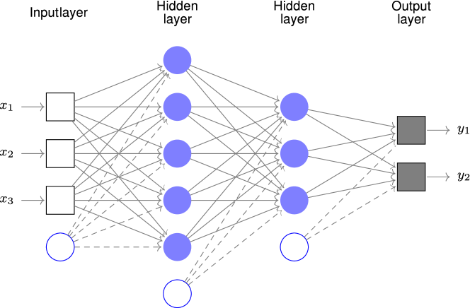
Figure 1: The above MLP contains two hidden unit layers. Empty squares denote the input, whereas filled circles represent the output; Blue filled and open circles indicate hidden and bias units, respectively.

We shall consider the feed-forward neural network in the multilayer perceptron (MLP) configuration. The MLP, denoted by $\mathcal{N}$, represents a nonlinear map from the input space of the dimension $d_{in}$ to the output space of the dimension $d_{out}$,

$$\mathcal{N}:\mathbb{R}^{d_{in}}\mapsto\mathbb{R}^{d_{out}}.$$ (1)

Note that $\mathcal{N}=\mathcal{N}(\mathbf{x},\textbf{w})$ is a function of input vector $\mathbf{x}\in\mathbb{R}^{d_{in}}$ and its parameters called weights, denoted by the vector $\textbf{w}=(w_{1},\dots,w_{i},\dots,w_{W})$, where $W$ is the total number of weights in a given network.

The MLP is represented by a graph consisting of several layers of connected units (nodes). Each edge of the graph corresponds to a function parameter, a weight, $w_{i}$. A unit (node) in a given layer is a single-valued function (activation function). Note that every unit, except the bias unit, is connected with the nodes from the previous layer. In a graph representing a neural network, we distinguish an input (input units), hidden layers of units, and an output layer. Each layer (except the output layer) has a bias unit connected only with the following layer units. It is a single-valued constant function equal to one. An example of a graph of a network with three-dimensional input and two-dimensional output is given in Fig. 1. This network has two hidden layers with five and three hidden units. The properties of the network, $\mathcal{N}$, are determined by its structure (architecture – topology of the connections) and the type of activation functions that settle in the neurons (units).

The universal approximation theorem [57, 58, 59] states that a feed-forward neural network with at least one layer of hidden units can approximate well any given continuous function. It is a fundamental property of neural networks used extensively in nonlinear regression and classification problems.

Note that the increasing number of units in the neural network broadens its adaptive abilities. However, if a network is large (contains many hidden units), then there is a danger that it can overfit the data, and as a result, it has low generalization abilities. On the other hand, if the network is small (low number of hidden units), it tends to underfit the data. This dilemma is known as the bias-variance trade-off [60]. There are some rules of thumb on how to solve the problem of under/over-fitting. The most popular is to constrain the values of the weight parameters by adding to the loss (6) the penalty term of the form:

$$E_{w}=\frac{\alpha}{2}\sum_{i=1}^{W}w_{i}^{2},$$ (2)

where $\alpha$ is the decay width parameter. There are other popular methods. However, we shall utilize the one described above because of its Bayesian interpretation. Note that we shall consider several decay width parameters accommodated in the vector $\boldsymbol{\alpha}$ below.

2.2 PINN: a formulation

We formulate the PINN approach similarly as in Ref. [61]. Let us consider the sets of equations:

$${Eq}_{i}(\mathbf{x},\hat{f},\partial\hat{f},\partial\partial\hat{f}) = 0,\quad i=1,2,\dots,q,\;\mathbf{x}\in\mathcal{M},$$ (3)

$$\mathcal{B}_{j}(\mathbf{x},\hat{f},\partial\hat{f}) = 0,\quad j=1,2,\dots,b,\;\mathbf{x}\in\partial\mathcal{M},$$ (4)

where ${Eq}_{i}$’s and $\mathcal{B}_{j}$’s are the differential and boundary operators respectively; $\mathcal{M}\subseteq\mathbb{R}^{d}$, $d=1,2,\dots$; $\hat{f}$ is the solution of the equations (3)-(4). Note that $\partial\hat{f}$ and $\partial\partial\hat{f}$ refer to any first-order partial derivative and second-order derivatives with respect to the input variables, respectively.

In the simplest version of the PINN approach, it is assumed that an approximate solution of the (3) with boundary conditions (4) is given by neural network $\mathcal{N}(\mathbf{x};\mathbf{w})$. Then, the network solution is so that

$$\mathbf{w}^{*}=\arg\min_{\mathbf{w}}E,$$ (5)

where

$$E = \frac{1}{2}\sum_{i=1}^{q}\beta_{q}^{i}\sum_{k=1}^{N_{q}}\left[{Eq}_{i}(\mathbf{x}_{k};\mathcal{N}(\mathbf{x}_{k},\mathbf{w}),\partial\mathcal{N}(\mathbf{x}_{k},\mathbf{w}),\partial\partial\mathcal{N}(\mathbf{x}_{k},\mathbf{w}))\right]^{2}$$ (6)

$$\!\!\!\!\!+\frac{1}{2}\sum_{j=1}^{b}\beta^{j}_{b}\sum_{k=1}^{N_{b}}\left[\mathcal{B}_{i}(\mathbf{x}_{k};\mathcal{N}(\mathbf{x}_{k},\mathbf{w}),\partial\mathcal{N}(\mathbf{x}_{k},\mathbf{w}),\partial\partial\mathcal{N}(\mathbf{x}_{k},\mathbf{w}))\right]^{2}.$$

The parameters $\beta^{i}_{q}$’s and $\beta^{j}_{b}$’s control the relative weights of the components of the loss $E$. To simplify the discussion, we shall consider only one $\beta^{i}_{q}=\beta_{q}$ and one $\beta^{j}_{b}=\beta_{b}$. We keep them together in the vector $\boldsymbol{\beta}=(\beta_{q},\beta_{b})$. Moreover, in this paper, we consider the PDEs with $q=1$. Hence the loss consists of

$$E_{D}^{q}=\frac{1}{2}\sum_{k=1}^{N_{q}}\left(Eq(\mathbf{x}_{k};\mathcal{N}(\mathbf{x}_{k},\mathbf{w}),\partial\mathcal{N}(\mathbf{x}_{k},\mathbf{w}),\partial\partial\mathcal{N}(\mathbf{x}_{k},\mathbf{w}))\right)^{2}$$ (7)

and

$$E_{D}^{b}=\frac{1}{2}\sum_{j=1}^{b}\sum_{k=1}^{N_{b}}\left(\mathcal{B}_{j}(\mathbf{x}_{k};\mathcal{N}(\mathbf{x}_{k},\mathbf{w}),\partial\mathcal{N}(\mathbf{x}_{k},\mathbf{w}),\partial\partial\mathcal{N}(\mathbf{x}_{k},\mathbf{w}))\right)^{2},$$ (8)

where

$$E=\beta_{q}E_{D}^{q}+\beta_{b}E_{D}^{b}$$ (9)

By $N_{q/b}$, we denote a number of points in $\mathcal{M}/\partial\mathcal{M}$ collected to optimize the network model. The total training dataset consists of points from $\mathcal{M}$ and $\partial\mathcal{M}$, namely, $\mathcal{D}=\mathcal{D}_{q}\cup\mathcal{D}_{b}$.

3 Bayesian framework for neural networks

Solving the PDE in the PINN approach comes down to optimization tasks. Namely, it is assumed that the neural network parameterizes the solution, then the loss, such as in Eq. 6, is formulated, and model parameters are optimized. Solving the PDE can be understood as the Bayesian inference process. Indeed, we assume prior knowledge about the solution and its parameters and then search for the posterior realization. Another problem is the proper fine-tuning of the beta parameters, which controls the impact of the boundary conditions on the solution. The choice of optimal network architecture seems to be essential too. Eventually, it is evident that the solution given by the neural network is only an approximation of the true solution, or it can be treated as a statistical prediction of the desired solution. Therefore, the PINN solution should be provided with uncertainties. We shall argue in the next section that the Bayesian statistical methods can help to establish the optimal structure of the network architecture; moreover, with the help of Bayesian reasoning, one may obtain the optimal values for the hyperparameters such as $\beta_{q}$ and $\beta_{b}$, and $\alpha$ (a decay width) and compute uncertainties for the obtained fits.

3.1 General foundations

The Bayesian Neural Network (BNN) framework [49, 50, 51, 32] we adapt aims to obtain the posterior densities for the network parameters, weights $\mathbf{w}$, and hyperparameters $\boldsymbol{\alpha}$ and $\boldsymbol{\beta}$.

A choice of network architecture impacts the analysis results. Indeed, the model, too simple, with a small number of neurons, cannot be flexible enough to describe the problem. On the other hand, the model too complex with many neurons tends to overfit the data. As we mentioned above BF shall allow us to compare fits obtained for different networks and get posterior densities for all necessary model parameters and hyperparameters.

In the BNN the posteriors for the model parameters and hyperparameters are obtained in the ladder approximation described below. Finally, the approach leads to the computation of the so-called evidence, a measure that ranks models.

The starting point of the procedure is to obtain the posterior density for the network weights. Assuming that the hyperparameters, $\boldsymbol{\alpha}$ and $\boldsymbol{\beta}$, and model architecture $\mathcal{N}$ are fixed

$$P(\mathbf{w}\mid\boldsymbol{\alpha},\boldsymbol{\beta},\mathcal{N},\mathcal{D}) = \frac{P(\mathcal{D}\mid\mathbf{w},\boldsymbol{\beta},\mathcal{N})P(\mathbf{w}\mid\boldsymbol{\alpha},\mathcal{N})}{P(\mathcal{D}\mid\boldsymbol{\alpha},\boldsymbol{\beta},\mathcal{N})}$$ (10)

$$P(\mathcal{D}\mid\boldsymbol{\alpha},\boldsymbol{\beta},\mathcal{N}) = \int P(\mathcal{D}\mid\mathbf{w},\boldsymbol{\beta},\mathcal{N})P(\mathbf{w}\mid\boldsymbol{\alpha},\mathcal{N})d\mathbf{w}$$ (11)

In the above, we silently assumed that the hyperparameter $\boldsymbol{\beta}$ appears in the likelihood $P(\mathcal{D}\mid\mathbf{w},\boldsymbol{\beta},\mathcal{N})$, while hyperparameter $\boldsymbol{\alpha}$ appears in prior $P(\mathbf{w}\mid\boldsymbol{\alpha},\mathcal{N})$ only.

In principle, the hyperparameters should be integrated out from the model’s prior densities, but it is not easy to perform. In the BNN framework, it is assumed that the posterior density $p(\boldsymbol{\alpha},\boldsymbol{\beta}\mid\mathcal{N},\mathcal{D})$ has a sharp peak at $\boldsymbol{\alpha}_{MP}$, $\boldsymbol{\beta}_{MP}$ ($MP$ - maximum of posterior) then prior for weights reads $p(\mathbf{w}\mid\mathcal{N},\mathcal{D})\approx p(\mathbf{w}\mid\boldsymbol{\alpha}_{MP},\boldsymbol{\beta}_{MP},\mathcal{N},\mathcal{D})$. We see that to obtain desired prior, one needs to find $\boldsymbol{\alpha}_{MP}$, $\boldsymbol{\beta}_{MP}$.

In the second step of the ladder, we use the likelihood for the hyperparameters, Eq. 11, to evaluate the posterior density for the hyperparameters, namely,

$$P(\boldsymbol{\alpha},\boldsymbol{\beta}\mid\mathcal{N},\mathcal{D}) = \frac{P(\mathcal{D}\mid\boldsymbol{\alpha},\boldsymbol{\beta},\mathcal{N})P(\boldsymbol{\alpha},\boldsymbol{\beta}\mid\mathcal{N})}{P(\mathcal{D}\mid\mathcal{N})}$$ (12)

$$P(\mathcal{D}\mid\mathcal{N}) = \int P(\mathcal{D}\mid\boldsymbol{\alpha},\boldsymbol{\beta},\mathcal{N})P(\boldsymbol{\alpha},\boldsymbol{\beta}\mid\mathcal{N})d\boldsymbol{\alpha}\,d\boldsymbol{\beta}$$ (13)

Note that the density (13) is called the model evidence. In reality, the prior for the hyperparameters factorizes into the product of two densities, namely,

$$P(\boldsymbol{\alpha},\boldsymbol{\beta}\mid\mathcal{N})=P(\boldsymbol{\alpha}\mid\mathcal{N})\,P(\boldsymbol{\beta}\mid\mathcal{N}).$$ (14)

In the third step, we compute the posterior density $P(\mathcal{N}\mid\mathcal{D})$. It is the quantity that ranks the models, i.e., a model the most favorable by the data has the highest value of $P(\mathcal{N}\mid\mathcal{D})$.

$$P(\mathcal{N}\mid\mathcal{D}) = \frac{P(\mathcal{D}\mid\mathcal{N})P(\mathcal{N})}{P(\mathcal{D})}.$$ (15)

In practice, any model is equally likely at the beginning of the analysis, and $P(\mathcal{N})$ is uninformative. Hence

$$P(\mathcal{N}\mid\mathcal{D}) \sim P(\mathcal{D}\mid\mathcal{N})$$ (16)

and to rank the model, it is enough to compute the evidence.

3.2 BNN framework

This section summarizes the main steps of the BNN framework. For more details, see chapter 10 of [32]. The main idea is to assume that all the densities should have a Gaussian-like shape.

Step 1

The prior density for the weights is constructed based on several observations. Namely, a network works the most efficiently for weights parameters that take values around zero. There are no sign preferences for the weights. Moreover, one can distinguish several classes of weights in the network. It is the result of the internal symmetries of a network model. For instance, the interchange of two units in the same hidden layer does not change the functional form of the network map. The weights which belong to the same class should have the same scaling property [32]. According to that, we assume the following Gaussian prior density for the weights:

$$p(\mathbf{w}\mid\boldsymbol{\alpha},\mathcal{N})=\frac{1}{Z_{W}}\exp\left(-\sum_{i=1}^{C}\alpha_{i}E_{w}^{i}\right)\equiv\frac{1}{Z_{W}}\exp\left(-E_{w}\right),$$ (17)

and

$$E_{w}^{i} = \frac{1}{2}\displaystyle\sum_{k=s_{i-1}}^{s_{i}}w_{k}^{2},\quad s_{i}=\sum_{l=1}^{i}W_{l},\;s_{0}=1$$ (18)

$$Z_{W}(\boldsymbol{\alpha}) = \prod_{i=1}^{C}\left(\frac{2\pi}{\alpha_{i}}\right)^{\frac{W_{i}}{2}},$$ (19)

In the above, $C$ denotes the number of weight classes; $w_{j}$ refers to the $j$-th weight, $W_{i}$ is the number of weights in $i$-th class; $\alpha_{i}$ is a decay width for $i$-th class of weights. The vector $\boldsymbol{\alpha}=(\alpha_{1},\dots,\alpha_{C})$ contains decay weights.

Note that the $\alpha_{i}$’s play two roles. They control the underfitting/overfitting. If $\alpha$ is too small, the network tends to overfit, whereas when $\alpha$ is too large, the network does not adapt to the data. The $1/\sqrt{\alpha_{i}}$’s defines the with of the Gaussian prior for weights.

Now, we shall construct the likelihood so that it contains all the contributions of the PINN loss terms. Assume that we have the constraints coming from the differential equations and one determined by the boundary condition, then we have two corresponding hyper-parameters $\beta_{q}$, $\beta_{b}$, and the likelihood reads

$$p(\mathcal{D}\mid\mathbf{w},\boldsymbol{\beta})=\frac{1}{Z_{D}(\boldsymbol{\beta})}\exp\left(-\beta_{q}E_{D}^{q}-\beta_{b}E_{D}^{b}\right),$$ (20)

where the normalization factor reads

$$Z_{D}(\boldsymbol{\beta})=Z_{D}(\beta_{q})Z_{D}(\beta_{b})$$ (21)

and

$$Z_{D}(\beta_{q(b)})=\left(\frac{2\pi}{\beta_{q(b)}}\right)^{\displaystyle\frac{N_{q(b)}}{2}}.$$ (22)

Having the posterior and the likelihood, we compute the posterior for the weights

$$p(\mathbf{w}\mid\mathcal{D},\boldsymbol{\alpha},\boldsymbol{\beta}) = \frac{p(\mathcal{D}\mid\mathbf{w},\boldsymbol{\beta})p(\mathbf{w},\boldsymbol{\alpha})}{\displaystyle\int d\mathbf{w}\,p(\mathcal{D}\mid\mathbf{w},\boldsymbol{\beta})p(\mathbf{w},\boldsymbol{\alpha})}$$ (23)

$$= \frac{1}{Z_{T}(\boldsymbol{\alpha},\boldsymbol{\beta})}\exp\left(-\left\{\sum_{i=1}^{C}\alpha_{i}E_{w}^{i}+\beta_{q}E_{D}^{q}+\beta_{b}E_{D}^{b}\right\}\right),$$ (24)

where

$$E_{T} = \sum_{i=1}^{C}\alpha_{i}E_{w}^{i}+\beta_{q}E_{D}^{q}+\beta_{b}E_{D}^{b}$$ (25)

$$Z_{T}(\boldsymbol{\alpha},\boldsymbol{\beta}) = \int d\mathbf{w}\exp\left(-E_{T}(\mathbf{w})\right).$$ (26)

Now it is assumed that the prior has a sharp local maximum. To obtain the posterior, one expands the $E_{T}$ around its minimum

$$E_{T}(\mathbf{w})\approx E_{T}(\mathbf{w}_{MP})+\frac{1}{2}\left(\mathbf{w}-\mathbf{w}_{MP}\right)^{T}\mathbf{A}\left(\mathbf{w}-\mathbf{w}_{MP}\right),$$ (27)

where $\mathbf{A}$ is defined by

$$\mathbf{A}=\mathbf{H}+\mathbf{I}_{W}({\boldsymbol{\alpha}}),$$ (28)

where

$$\mathbf{I}_{W}({\boldsymbol{\alpha}})=\mathrm{diag}(\underbrace{\alpha_{1},\dots,\alpha_{1}}_{W_{1}\,times},\dots,\underbrace{\alpha_{C},\dots,\alpha_{C}}_{W_{C}\,times})$$ (29)

and

$$\mathbf{H}_{ij}=\beta_{q}\nabla_{i}\nabla_{j}E_{D}^{q}+\beta_{b}\nabla_{i}\nabla_{j}E_{D}^{b}$$ (30)

is the Hessian.

Within the above approximation, one gets:

$$p(\mathbf{w}\mid\mathcal{D},\boldsymbol{\alpha},\boldsymbol{\beta})=\frac{1}{Z_{E_{T}}^{*}}\exp\left(-E_{T}(\mathbf{w}_{MP})-\frac{1}{2}\left(\mathbf{w}-\mathbf{w}_{MP}\right)^{T}\mathbf{A}\left(\mathbf{w}-\mathbf{w}_{MP}\right)\right),$$ (31)

where $Z_{E_{T}}\to Z_{E_{T}}^{*}$,

$$Z_{E_{T}}^{*}=\exp\left(-E_{T}(\mathbf{w}_{MP})\right)\sqrt{\frac{(2\pi)^{W}}{|\mathbf{A}|}}.$$ (32)

$|\mathbf{A}|$ is determinant of matrix $\mathbf{A}$. Eventually, we obtain the posterior

$$p(\mathbf{w}\mid\mathcal{D},\boldsymbol{\alpha},\boldsymbol{\beta})=\sqrt{\frac{|\mathbf{A}|}{(2\pi)^{W}}}\exp\left(-\frac{1}{2}\left(\mathbf{w}-\mathbf{w}_{MP}\right)^{T}\mathbf{A}\left(\mathbf{w}-\mathbf{w}_{MP}\right)\right).$$ (33)

Note that to find the $\mathbf{w}_{MP}$, we shall find the minimum of the loss (25).

Step 2

We search for the hyperparameters $\boldsymbol{\alpha}_{MP}$, $\boldsymbol{\beta}_{MP}$ that maximize the posterior $p(\boldsymbol{\alpha},\boldsymbol{\beta}\mid\mathcal{N},\mathcal{D})$ but because there is no prior knowledge about them usually the non-informative priors are dicussed [62]. Hence the density $p(\mathcal{D}\mid\boldsymbol{\alpha},\boldsymbol{\beta},\mathcal{N})$ should has the peak in the same position as $p(\boldsymbol{\alpha},\boldsymbol{\beta}\mid\mathcal{N},\mathcal{D})$. Than we compute

$$p(\mathcal{D}\mid\boldsymbol{\alpha},\boldsymbol{\beta},\mathcal{N})=\int d\mathbf{w}p(\mathcal{D}\mid\mathbf{w},\boldsymbol{\beta})p(\mathbf{w}\mid\boldsymbol{\alpha},\mathcal{N})=\frac{Z_{E_{T}}^{*}}{Z_{D}(\boldsymbol{\beta})Z_{W}(\boldsymbol{\alpha})},$$ (34)

where it was assumed that prior depends only on $\boldsymbol{\alpha}$ whereas the likelihood on $\boldsymbol{\beta}$ only. Then one gets

$$\ln p(\mathcal{D}\mid\boldsymbol{\alpha},\boldsymbol{\beta},\mathcal{N}) \approx -\sum_{i=1}^{C}\alpha_{i}E_{w}^{i}(\mathbf{w}_{MP})-\beta_{q}E_{D}^{q}(\mathbf{w}_{MP})-\beta_{b}E_{D}^{q}(\mathbf{w}_{MP})$$

$$\!\!\!\!\!\!\!\!\!\!\!\!\!\!\!\!\!\!\!\!\!\!\!\!\!\!\!\!\!\!-\frac{1}{2}\ln|\mathbf{A}|-\sum_{i=1}^{C}\frac{W_{i}}{2}\ln\left(\frac{2\pi}{\alpha_{i}}\right)-\frac{N_{q}}{2}\ln\left(\frac{2\pi}{\beta_{q}}\right)-\frac{N_{b}}{2}\ln\left(\frac{2\pi}{\beta_{b}}\right).$$

We search for the maximum of $p(\mathcal{D}\mid\boldsymbol{\alpha},\boldsymbol{\beta},\mathcal{N})$, in the original MacKay’s framework, the hyper-parameters are iterated according to the necessary condition for the maximum, namely from the equations:

$$\frac{\partial}{\partial\boldsymbol{\alpha}}p(\mathcal{D}\mid\boldsymbol{\alpha},\boldsymbol{\beta},\mathcal{N})=0,\quad\frac{\partial}{\partial\boldsymbol{\beta}}p(\mathcal{D}\mid\boldsymbol{\alpha},\boldsymbol{\beta},\mathcal{N})=0.$$

In our approach, we propose to consider additional loss given by $E_{hyp}=-\ln p(\mathcal{D}\mid\boldsymbol{\alpha},\boldsymbol{\beta})$ and optimize it with respect to hyperparameters. The loss, after neglecting constant terms, has the form

$$E_{hyp} = \sum_{i=1}^{C}\alpha_{i}E_{w}^{i}(\mathbf{w}_{MP})+\beta_{q}E_{D}^{q}(\mathbf{w}_{MP})+\beta_{b}E_{D}^{b}(\mathbf{w}_{MP})+\frac{1}{2}\ln|\mathbf{A}|$$ (36)

$$-\sum_{i=1}^{C}\frac{W_{i}}{2}\ln\alpha_{i}-\frac{N_{q}}{2}\ln\beta_{q}-\frac{N_{b}}{2}\ln\beta_{b}.$$

Step 3

To compute the evidence, one has to integrate out the hyperparameters from $p(\mathcal{D}\mid\boldsymbol{\alpha},\boldsymbol{\beta},\mathcal{N})$ using the similar arguments as for the prior for the weights, namely, the posterior for the hyperparameters has a sharp peak in their parameters. As it is argued in [32, 62] are the scaling parameters that are always positive. Therefore, instead of considering $p(\mathcal{D}\mid\boldsymbol{\alpha},\boldsymbol{\beta},\mathcal{N})\boldsymbol{d}\alpha\boldsymbol{d}\beta$, one discusses $p(\mathcal{D}\mid\ln\boldsymbol{\alpha},d\ln\boldsymbol{\beta},\mathcal{N})d\boldsymbol{\ln}\alpha\boldsymbol{\ln}\beta$. Then it is assumed that the prior for $\ln$ of hyperparameters is flat. As a result, the log of evidence reads

$$\ln p(\mathcal{D}\mid\mathcal{N})=\ln p(\mathcal{D}\mid\boldsymbol{\alpha},\boldsymbol{\beta})+\ln\sigma_{\ln\alpha}+\ln\sigma_{\ln\beta_{Eq}}+\ln\sigma_{\ln\beta_{b}}+comb,$$ (37)

where

$$\ln p(\mathcal{D}\mid\boldsymbol{\alpha},\boldsymbol{\beta}) = -\sum_{i=1}^{C}\alpha_{i}E_{w}^{i}(\mathbf{w}_{MP})-\beta_{Eq}E_{D}^{q}(\mathbf{w}_{MP})-\beta_{b}E_{D}^{B}(\mathbf{w}_{MP})$$ (38)

$$-\frac{1}{2}\ln|\mathbf{A}|+\sum_{i=1}^{C}\frac{W_{i}}{2}\ln\alpha_{i}+\frac{N_{q}}{2}\ln\beta_{q}+\frac{N_{b}}{2}\ln\beta_{b}$$

and

$$\ln{\sigma_{\ln\alpha_{i}}} = -\frac{1}{2}\ln\left[-\alpha^{2}_{i}\frac{\partial^{2}}{\partial\alpha_{i}^{2}}\ln p(\mathcal{D}\mid\boldsymbol{\alpha},\boldsymbol{\beta})\right]$$ (39)

$$\ln{\sigma_{\ln\beta_{i}}} = -\frac{1}{2}\ln\left[-\beta^{2}_{i}\frac{\partial^{2}}{\partial\beta_{i}^{2}}\ln p(\mathcal{D}\mid\boldsymbol{\alpha},\boldsymbol{\beta})\right].$$ (40)

The expression (37) consists of the symmetry contribution, as discussed in Ref. [63], namely,

$$comb=\sum_{i=1}^{L}\left(\ln M_{i}!+M_{i}\ln 2\right),$$ (41)

where $M_{i}$ denotes number of units in the $i$-th hidden layer, $L$ denotes number of hidden layers.

Uncertainty for the network predictions

We compute the uncertainty for network predictions in the covariance matrix approximation. The $1\sigma$ uncertainty due to the variation of the weights reads [64]

$$\Delta^{2}\mathcal{N}(\mathbf{x}_{q(b)},\mathbf{w}_{MP})=\sum_{i,j}\nabla_{i}\mathcal{N}(\mathbf{x}_{q(b)},\mathbf{w}_{MP})\;(\mathbf{A}^{-1})_{ij}\nabla_{j}\mathcal{N}(\mathbf{x}_{q(b)},\mathbf{w}_{MP}),$$ (42)

where $\mathbf{x}_{q(b)}$ refers to point from $\mathcal{M}(\partial\mathcal{M})$; $\nabla_{i}\equiv\partial/\partial w_{i}$.

3.3 Training algorithm

Here we shortly summarize the training algorithm.

• Set the network architecture and initial values for the weights.

• Set initial values of $\mathbf{\alpha}_{i}=\mathbf{\alpha}_{i}^{(0)}$ and $\mathbf{\beta}_{a}=\mathbf{\beta}_{a}^{(0)}$.

• To get $\mathbf{w}^{*}$ minimize the loss (25).

• To get hyperparameters $\mathbf{\alpha}$ and $\mathbf{\beta}$ minimize the loss (36).

• The best network has the highest evidence value computed from (37).

Note that during the training process, one has to update weights and the values of hyperparameters simultaneously. But it turned out that to maintain the convergence of the process, we had to start optimizing $\alpha$’s and $\beta$’s several epochs after we started optimizing the weights.

4 Numerical experiments

We shall solve three types of PDEs: heat, wave, and Burger’s equations. For the first two, the analytic solutions are known. For the last one, there is no analytical solution. Our approach is implemented using PyTorch framework [56]. We collected $100$ of solutions for each PDEs to choose the best one according to the evidence.

4.1 Heat equation

Let us consider the heat equation of the form

$$\frac{\partial u}{\partial t}-\kappa\frac{\partial^{2}u}{\partial x^{2}} = 0,\quad x\in[0,1],\;\;t\in[0,1],$$ (43)

$$u(0,t)=u(1,t) = 0,$$ (44)

$$u(x,0) = \sin(\pi x)$$ (45)

For the above case the analytic solution reads $u_{\text{true}}(x,t)=\sin(\pi x)\exp(-\kappa\pi^{2}t)$.

We consider the network with three layers of units to solve the heat equation (43) with boundary conditions (44-45). Each hidden layer has $16$ neurons with hyperbolic tangent activation functions. In the output layer, there are linear activation functions.

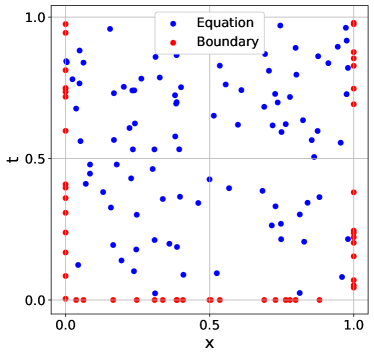
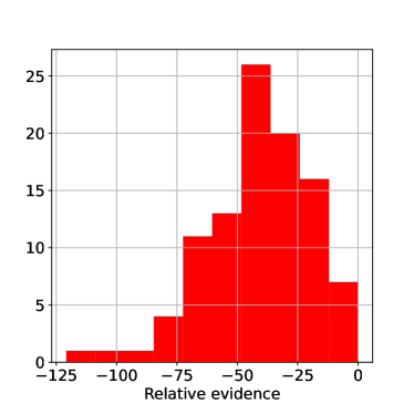
Figure 2: In the left panel: the training data, the blue/red points correspond to the equation/boundary contribution to the loss for the heat equation. In the right panel: the histogram of the relative log of evidence (the difference between a given log of evidence and the highest log of evidence).

The data on the boundary Eqs. (44-45) were randomly drawn from the uniform distribution ($50$ points). Similarly, we obtained data in $(0,1)\times(0,1)$ (100 points). The data considered in the training are shown in Fig. 2 (left panel). The model was optimized within the AdamW algorithm run for about $800$ epochs. The AdamW was also utilized to optimize $alpha$ and $\beta$. The Bayesian training was performed in the simplest fashion. Namely, we kept one $\alpha$ parameter for all weight classes (as in Ref. [3]) and one $\beta=\beta_{q}=\beta_{b}$ for equation and boundary contribution.

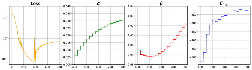
Figure 3: An example of loss $E_{T}$ (the first panel in the left), $E_{hyp}$ (the last panel) and $\alpha$ (the second from the right) and $\beta$ (the third from the right) hyperparameters evolution during the training of the network that solves the heat equation.

We optimized the hyperparameters after $400$ epochs to maintain the procedure’s convergence. Then every $25$ epoch, we updated the $\alpha$ and $\beta$ parameters to minimize the error $E_{hyp}$. In Fig. 3, we show one of the registered training examples. The method leads to the convergence of both discussed losses $E_{T}$ (with respect to weights) and $E_{hyp}$ with respect to hyperparameters. We started the optimization from a low value of $\alpha$ (minor relevance of the penalty term). During the training, $\alpha$ changes by the order of magnitude. The $\beta$ parameter slowly varies during the optimization process.

For every fit, we compute the evidence. In Fig. 2 (right panel), we show the histogram of evidence values for $100$ models. The best model has the highest evidence. In Fig. 4 we show our best fit together with the exact analytic solution. The fit is plotted together with uncertainty. Note that we show the $x$-dependence of the solution in five time steps.

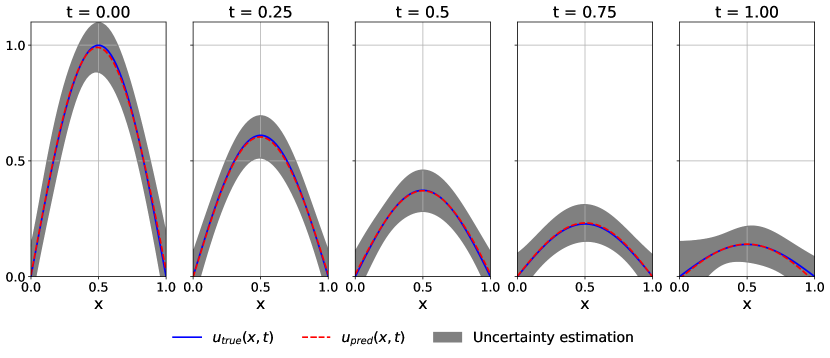
Figure 4: The exact ($u_{true}$) and PINN ($u_{pred}$) solutions for the heat equation.

4.2 Wave equation

Let us consider the following wave equation

$$\frac{\partial^{2}u}{\partial t^{2}}-\frac{\partial^{2}u}{\partial x^{2}} = 0,\quad x\in[0,1],\;t\in[0,1]$$ (46)

$$u(0,t)=u(1,t) = 0$$ (47)

$$\frac{\partial}{\partial t}u(0,t) = 0$$ (48)

with

$$u(x,0)=\sin(\pi x)+\frac{1}{2}\sin(2\pi x).$$ (49)

or

$$u(x,0)=\sin(\pi x)$$ (50)

For the Eqs. (46) (47), (48) and either (49) or (50) the analytic solution reads either $u_{\text{true}}(x,t)=\sin(\pi x)\cos(\pi t)+\frac{1}{2}\sin(2\pi x)\cos(2\pi t)$ or $u_{\text{true}}(x,t)=\sin(\pi x)\cos(\pi t)$, respectively.

As demonstrated in the previous subsection, the BNN framework works well for the heat equation. Indeed, to find the solution, it was enough to consider rather a small network, and the optimization took a relatively small number of epochs. Solving the wave equation with BNN turned out to be more challenging. In this case, we consider a network with four hidden layers. Each layer has $16$ hidden units. The hyperbolic tangent as an activation function is set for the hidden units. We generated a larger data set for the heat equation case to obtain successful fits. Namely, we drew from a uniform distribution $500$ and $100$ points for $\mathcal{M}$ and $\partial\mathcal{M}$, respectively. We show the distribution of dataset in the left panel of Fig. 5.

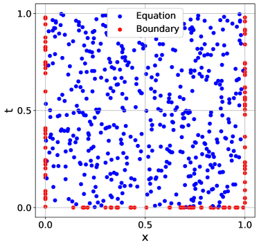
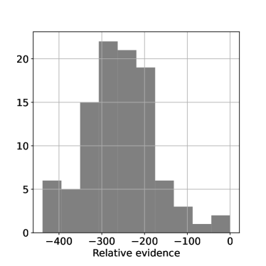
Figure 5: In the left panel: the training data, the blue/red points correspond to equation/boundary contribution to the loss for the wave equation. In the right panel: the histogram of the relative log of evidence (the difference between a given log of evidence and the highest log of evidence).

The wave equation with boundary condition (49) was solved in the simplified framework with only one $\alpha$ and $\beta$ hyperparameters. For this case, the learning process lasted significantly longer than the heat equation and took more than $3000$ epochs. We started optimization of the hyperparameters in the $1500$th epoch. However, because the computation time of the Hessian took quite a long time, we started taking into account the covariance matrix term in the $E_{Hyp}$ above $2500$ epochs when the algorithm was close to the minimum of 25. The training example for this case is given in Fig. 6.

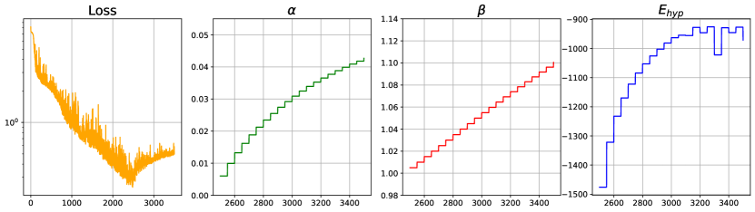
Figure 6: An example parameters evolution during the wave equation training

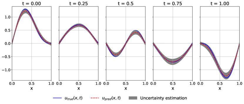
Figure 7: The exact ($u_{true}$) and PINN ($u_{pred}$) solutions for the heat equation with boundary conditions (49).

Similarly, as for the heat equation, we show the histogram of the relative log of evidence values in the right panel of Fig. 5. Our best fit agrees with the true solution; see Fig. 7. However, one can notice a slight difference between the wave equation’s exact and network model solutions. To visualize this feature, we plot $u_{true}(x,t)-u_{pred}(x,t)$ together with uncertainty in Fig. 8.

Figure 8: Comparison of the obtained uncertainties and real error for the solution of the wave equation with boundary condition (49). The $y=0$ axes correspond to the exact agreement between ”true” and network solutions, and it is included, for practically all $x$, in the confidence interval marked by the grey area.

Keeping more than one $\alpha$ and $\beta$ parameters complicates the numerical computation, making it more challenging to obtain convergence. However, for the wave equation with simpler boundary conditions (50) we performed complete analysis, keeping for every layer of units weights one $\alpha$ and separate $\alpha$ for bias unit. We also hold two betas, namely $\beta_{q}$ for the equation and $\beta_{b}$.

To perform the analysis, we prepared the dataset containing $50$ points for $\mathcal{M}$ and $50$ points for $\partial\mathcal{M}$. The training was enclosed in $1500$ epochs. The optimization of hyperparameters started in the $750$th epoch. The neural network contained three hidden layers with $16$ neurons each, so we had $8$ $\alpha$ parameters (two for each layer: one for ordinary weights, and one for bias weights). We obtained the fit that agrees with the true solution; see Fig. 9.

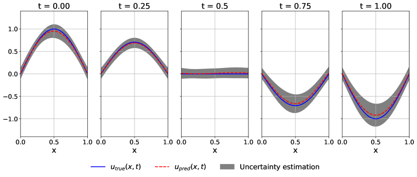
Figure 9: The exact ($u_{true}$) and PINN ($u_{pred}$) solutions for the wave equation with boundary conditions (50).

4.3 Burger’s equation

For the last example of PDEs, we consider Burger’s equation with Dirichlet boundary conditions.

$$\frac{\partial u}{\partial t}+u\,\frac{\partial u}{\partial x}-\frac{1}{100\pi}\frac{\partial^{2}u}{\partial x^{2}} = 0,\quad x\in[-1,1],\;\;t\in[0,1]$$ (51)

$$u(0,x) = -\sin(\pi x)$$ (52)

$$u(t,-1) = u(t,1)=0$$ (53)

It is the same equation as discussed in Ref. [11].

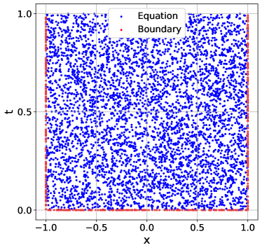
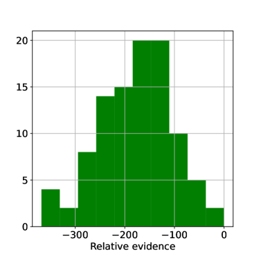
Figure 10: In the left panel: the training data, the blue/red points correspond to the equation/boundary contribution to the loss for Burger’s equation. In the right panel: the histogram of the relative log of evidence (the difference between a given and highest log of evidence).

Burger’s equation is the most difficult to solve among the three PDEs discussed in this paper. To find the solution, we consider a network with four hidden layers of units. In each layer, there are $20$ hidden neurons. The dataset contains $5000$ and $1000$ for $\mathcal{M}$ and $\partial\mathcal{M}$, respectively. We show the data distribution in Fig. 10 (left panel). The network is trained in a mini-batch configuration (10 batches for each epoch). Similarly, we collected $100$ fits for two previous PDEs examples. The histogram of the log of evidence for collected fits is given in Fig. 10 (right panel). In Fig. 11, we show our best fit with the numerical solution obtained in Ref. [11]. A good agreement between the predictions of both approaches is seen.

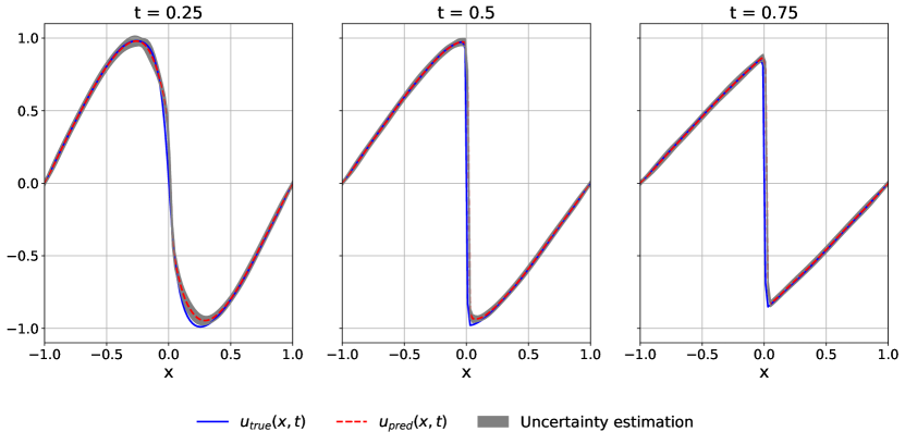
Figure 11: The ”true” solution ($u_{true}$) - the numerical solution from [11]), and our best model predictions ($u_{pred}$) for Burger’s equation.

5 Summary

We adopted the Bayesian framework for the PINN to solve heat, wave, and Burger’s equations. The network solutions agree with the ”true” ones. The method allowed us to compute the $1\sigma$ uncertainty due to variation of network parameters. We have demonstrated (for the wave equation problem) that the relative weights of the loss components, such as the boundary condition loss term, can be treated as the model’s hyperparameters and fined-tuned within the Bayesian algorithm. Indeed, the network parameters, weights, and hyperparameters were optimized in parallel during the training process. One of the merits of the Bayesian framework is that there is no need to use the validation data set. The entire collected data can be utilized in the analysis. However, when the network is defined by a large number of weights, the numerical evaluation of the Hessian takes a long time and is imprecise. In this case, the method might work ineffectively. However, for small-size networks, the discussed Bayesian approach works well.

References

-
[1]
Y. LeCun, Y. Bengio, G. Hinton, Deep
learning, Nature 521 (2015) 436 EP –.
URL https://doi.org/10.1038/nature14539 -
[2]
P. Mehta, M. Bukov, C.-H. Wang, A. G. Day, C. Richardson, C. K. Fisher, D. J.
Schwab,
A
high-bias, low-variance introduction to machine learning for physicists,
Physics Reports 810 (2019) 1 – 124, a high-bias, low-variance introduction
to Machine Learning for physicists.
doi:https://doi.org/10.1016/j.physrep.2019.03.001.
URL http://www.sciencedirect.com/science/article/pii/S0370157319300766 - [3] K. M. Graczyk, P. Plonski, R. Sulej, Neural Network Parameterizations of Electromagnetic Nucleon Form Factors, JHEP 09 (2010) 053. arXiv:1006.0342, doi:10.1007/JHEP09(2010)053.
- [4] K. M. Graczyk, C. Juszczak, Proton radius from Bayesian inference, Phys. Rev. C90 (2014) 054334. arXiv:1408.0150, doi:10.1103/PhysRevC.90.054334.
- [5] K. M. Graczyk, M. Matyka, Predicting porosity, permeability, and tortuosity of porous media from images by deep learning, Scientific reports 10 (1) (2020) 1–11.
-
[6]
J.-L. Wu, H. Xiao, E. Paterson,