Physics-Inspired Neural Graph ODE for
Long-term Dynamical Simulation

Abstract

Simulating and modeling the long-term dynamics of multi-object physical systems is an essential and challenging task. Current studies model the physical systems utilizing Graph Neural Networks (GNNs) with equivariant properties. Specifically, they model the dynamics as a sequence of discrete states with a fixed time interval and learn a direct mapping for all the two adjacent states. However, this direct mapping overlooks the continuous nature between the two states. Namely, we have verified that there are countless possible trajectories between two discrete dynamic states in current GNN-based direct mapping models. This issue greatly hinders the model generalization ability, leading to poor performance of the long-term simulation. In this paper, to better model the latent trajectory through discrete supervision signals, we propose a Physics-Inspired Neural Graph ODE (PINGO) algorithm. In PINGO, to ensure the uniqueness of the trajectory, we construct a Physics-Inspired Neural ODE framework to update the latent trajectory. Meanwhile, to effectively capture intricate interactions among objects, we use a GNN-based model to parameterize Neural ODE in a plug-and-play manner. Furthermore, we prove that the discrepancy between the learned trajectory of PIGNO and the true trajectory can be theoretically bounded. Extensive experiments verify our theoretical findings and demonstrate that our model yields an order-of-magnitude improvement over the state-of-the-art baselines, especially on long-term predictions and roll-out errors.

1 Introduction

It is a vital problem to simulate and model the complex dynamics of multi-object physical systems, i.e. N-body systems. This problem is relevant to numerous fundamental scientific domains, including molecular dynamics [19], protein folding [11], drug and catalyst virtual screening [32], robot motion planning/control [30], and cosmological simulation [34].

Because of the complex interaction of multiple objects in the N-body system, recent studies propose to use Graph Neural Networks (GNNs) [28, 10] to model the N-body systems. Specifically, they model the objects in the physical system as nodes, the physical relations as edges, and use a message-passing network to learn interactions among nodes. Recently, some works try to encode the physical symmetry into GNNs to ensure the translating/rotating/reflecting equivariant between the geometric input and output of GNN. These models are known as equivariant GNNs [28, 14, 3, 15] and have emerged as a type of leading approaches for N-body system modeling. Most of the existing studies on equivariant GNNs treat the dynamic process as a sequence of discrete states, encompassing the positions, velocities, and forces of each object. Then given an input state, a direct mapping is learned by constraining the model output to approximate the next adjacent state after the input one, over a fixed time interval. We refer to this type of method as direct-mapping models.

However, we question the validity of the direct-mapping models on two fronts. Firstly, models derived from this paradigm exhibit limited generalizability over time. Specifically, it is possible to apply models trained on short-term data for predictions on longer time intervals through rollout, but not vice versa. Secondly, a direct-mapping model can not capture the continuous physical knowledge between discrete states. To verify this, we train multiple EGNN models with different random seeds on a 3-body system with two adjacent stats $t_{0},t_{1}$. We extract the object positions from their hidden layers, as the estimation of intermediate motion trajectories between two status $t_{0.5}$, and perform one-step rollouts to make the prediction of next state $t_{2}$. We visualize all predicted trajectories (in dotted grey), the mean trajectory (in blue), and the mean and variance of predicted stats in the left part of Figure $\dagger$ ‣ 1 (a). As shown in Figure $\dagger$ ‣ 1 (a), the predictions of EGNN have a high variance at both intermediate and rollout states, indicating that the direct-mapping models are unable to learn a uniquely determined motion trajectory. This is a crucial reason why existing models struggle with long-term physical simulations.

In this paper, to better model the latent motion trajectory under discrete supervision signals, we propose Physics-Inspired Neural Graph Ordinary Differential Equation, dubbed PINGO. Unlike the direct-mapping models which use GNNs to fit all kinematic states, PINGO introduces a Neural ODE framework built upon motion equations to update the position and velocity of the physical system. Theoretically, we prove the uniqueness of the learned latent trajectory of this framework and further provide an upper bound on the discrepancy between the learned and the actual latent trajectory. Figure $\dagger$ ‣ 1 (a) also depicts an example of prediction results of the latent trajectory of PINGO, following the same training protocol of EGNN. PINGO achieves a significant small variance on both the intermediate and rollout state, and it coincides with the true latent trajectory. Meanwhile, we employ a GNN model to parameterize the force relationships in the Neural ODE framework. Owing to the GNNs’ expressive power, PINGO can adeptly address the force prediction issues for each object in the system. Figure $\dagger$ ‣ 1 (b) shows the key difference between PINGO and direct-mapping methods. Moreover, we provide theoretical proof that PINGO exhibits equivariance properties identical to those of the input GNN model. This property offers the flexibility to adapt various GNN backbones in PINGO to suit different downstream tasks. We conduct extensive experiments on both synthetic and real world physical systems. The results shows that PINGO have an order-of-magnitude improvement over the state-of-the-art baselines on both direction prediction and rollout setting, especially for the extreme long-term simulation.

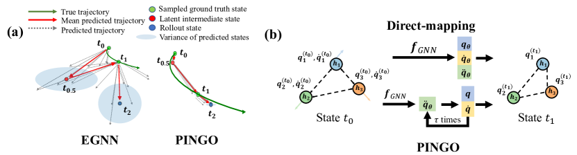
Figure 1: (a) Comparison of the trajectory prediction of EGNN and PINGO. The green line is the true trajectory extracted from a 3-body system. The dotted grey line is the predicted trajectory from the same model with different random seeds. The red line is the average trajectory aggregated by the predicted trajectories. The green circle ($t_{0},t_{1}$) is the ground truth state used for training. The red circle ($t_{0.5}$) is the predicted latent state from the average trajectory. The dark blue circle ($t_{2}$) is the predicted rollout state. The blue area is the variance of the predicted latent state and rollout state. (b) The overview of PINGO. $\bm{q},\dot{\bm{q}}$ and $\ddot{\bm{q}}$ represent the position, velocity, and acceleration (force), respectively.

2 Related Works

GNNs for Modeling the Dynamics of N-body Systems

Interaction Network (IN)[1] is a pioneer work that models objects and relations as graphs and applies multi-step rollouts to make predictions. After that, several studies [21, 24, 27] leverage GNNs and their variants to explicitly reason about the dynamics behind object interactions. Recently, researchers have introduced physical symmetry into models of interacting objects of physical system. For example, TFN [31] and SE(3) Transformer [9] employ spherical harmonics to construct models with 3D rotation equivariance in the Euclidean group for higher-order geometric representations. LieConv [7] and LieTransformer [18] leverage the Lie convolution to extend equivariance on Lie groups. In addition to these methods, which rely on irreducible representations of certain symmetry groups, recent studies [28, 15, 29] apply scalarization techniques to introduce equivariance into the message-passing process in GNNs. Furthermore, SEGNN [3] generalizes EGNN [28] and extends invariant scalars on nodes/edges to covariant vectors and tensors. Finally, EGHN [14] extends the framework of GMN [15] to design equivalent pooling and up-pooling modules for hierarchical modeling of large-scale dynamic systems, such as proteins. Nevertheless, these methods model dynamics in physical systems solely by learning direct mappings between discrete states and conducting long-term simulations via the rollout method.

Physics-Inspired Neural Networks

Infusing physical knowledge has been shown to improve learning neural networks for dynamical system modeling. Broadly speaking, energy conservation, symplectic nature, and ODE are three common physical biases. Our work focuses on ODE bias which models derivatives of the state rather than the states directly. Representation models include Lagrangian Neural Networks (LNN) [8, 23], Hamiltonian neural networks (HNN) [12], and Neural ODE [4, 13]. Recent studies [25, 26, 2] have Integrated Neural ODE and GNNs to learn the motion of interactive particles. Graph Neural Ordinary Differential Equation [25] uses graph convolutional networks to parameterize the first- and second-order derivatives of system states. A concurrent work [2] directly uses actual acceleration to train GNNs. However, how they approximate the system trajectory is still an open problem. Motivated by the physical laws, we theoretically justify how our approach can improve the generalization ability in the time dimension and quantify the error brought by the discrete ODE solver. Another research line [17, 16, 35, 33, 36] employs GNN and the first-order Neural ODE to produce smooth trajectories of multi-agent systems. They validate these methods on complex irregularly sampled and partially observed systems in COVID-19 and social scenarios. In contrast, our work lies in the strong approximation ability of the second-order Neural ODE and equivariant GNNs to learn the dynamics of physical systems.

3 Preliminary

N-body System

We study N-body systems [21, 15] with a set of objects $\mathcal{P}=\{P_{i}\}_{i=1}^{N}$. At time $t$, the state of the system is represented by its geometric feature $(\bm{q}^{(t)},\bm{\dot{q}}^{(t)})$, where $\bm{q}^{(t)}\in\mathbb{R}^{N\times 3}$ and $\bm{\dot{q}}^{(t)}\in\mathbb{R}^{N\times 3}$ are the position and the velocity vector, respectively, for the object $P_{i}$. Additionally, objects $P$ are associated with non-geometric attributes such as mass or charge, which is denoted by $\bm{h}\in\mathbb{R}^{N\times d}$. We use a graph $\mathcal{G}=\{\mathcal{P},\mathcal{E}\}$ to represent the spatial connections in the system where $\mathcal{E}$ is an edge set that is constructed via geometric distance cutoff or physical connectivity. The attributes of edge $e_{ij}\in\mathcal{E}$ (e.g., object distances) are denoted by $a_{ij}$. The system state at time $t$ is abbreviated as $\mathcal{S}^{(t)}=(\mathcal{G},\bm{q}^{(t)},\bm{\dot{q}}^{(t)},\bm{h})$. Since the predictions at different times share the same model, without ambiguity, we will omit the temporal superscript $t$ for all variables for brevity when necessary.

Physical Background

According to Newton’s second law, “When a body is acted upon by force, the time rate of change of its momentum equals the force”. For physical systems that follow Newtonian mechanics, their motion can be described by the following general ordinary differential equation

$$\bm{\ddot{q}}^{(t)}=\frac{d^{2}\bm{q}^{(t)}}{dt^{2}}=f(t,\bm{q}^{(t)},\bm{\dot{q}}^{(t)},\bm{h}).$$ (1)

In this work, we focus on dynamical systems that can be formulated as:

$$\bm{\ddot{q}}^{(t)}=f(\bm{q}^{(t)},\bm{h}),$$ (2)

where $\bm{\ddot{q}}^{(t)}$ is the acceleration at time $t$. If we have a closed-form solution of $f$, given the initial position $\bm{q}^{(t_{0})}$ and velocity $\bm{\dot{q}}^{(t_{0})}$ at time $t_{0}$, the position at time $t_{1}>t_{0}$ can be obtained by integrating the above differential equation:

$$\bm{q}^{(t_{1})}=\bm{q}^{(t_{0})}+\int_{t_{0}}^{t_{1}}(\bm{\dot{q}}^{(t_{0})}+\int_{t_{0}}^{t}\bm{\ddot{q}}^{(m)}\,dm)\,dt=\bm{q}^{(t_{0})}+\int_{t_{0}}^{t_{1}}g(\bm{q}^{(t)},\bm{h})\,dt.$$ (3)

Under the aforementioned assumptions, we have

$$\bm{\dot{q}}^{(t)}=g(\bm{q}^{(t)},\bm{h}).$$ (4)

But such a solution is not generally available, especially when the system is complex. Thus, current works are interested in learning a graph neural network to directly approximate $\bm{q}^{(t_{1})}$ on observed system trajectories.

GNN-based Direct-mapping Model

Existing studies seek to use a GNN to directly approximate the above unavailable integration results with training pairs $\left(\bm{q}^{(t_{0})},\bm{q}^{(t_{1})}\right)$. Namely, given the system state at time $t_{0}$, modern GNN simulators $\psi_{\theta}$ with parameters $\theta$ predicts $\bm{q}^{(t_{1})}$ and update node features via message passing. Specifically, each layer of $\psi_{\theta}$ computes

$$\bm{q^{\prime}}_{i},\bm{\dot{q}^{\prime}}_{i},\bm{h^{\prime}}_{i} =\varphi(\bm{q}_{i},\bm{\dot{q}}_{i},\bm{h}_{i},\sum_{j\in\mathcal{N}_{i}}\bm{m_{ij}}),\qquad\bm{m_{ij}} =\phi(\bm{q}_{i},\bm{q}_{j},\bm{\dot{q}}_{i},\bm{\dot{q}}_{j},\bm{h}_{i},\bm{h}_{j},a_{ij}),$$ (5)

where $\phi$ and $\varphi$ are the edge message function and node update function, respectively, which typically are MLPs. $\bm{q}_{i},\bm{\dot{q}}_{i}\in\mathbb{R}^{3}$ and $\bm{h}_{i}\in\mathbb{R}^{d}$ are the features of particle $P_{i}$. $\bm{m_{ij}}$ defines the message between node $i$ and $j$. $\mathcal{N}_{i}$ collects the neighbors of node $i$. The prediction is obtained by applying several iterations of message passing. Although the direct method precisely predicts the state of object dynamics with the interval $T=t_{1}-t_{0}$, its prediction with other intervals is notably inconsistent and suboptimal.

Problem Definition

This study concentrates on the temporal generalization capacity of the model. Adopting established approaches, the model is trained to predict the subsequent position $\bm{q}^{(t_{1})}$ as accurately as feasible, considering the system state at time $t_{0}$. Additionally, the model is capable of (1) accurately predicting unobserved intermediate time points by further uniformly partitioning the time interval $T=t_{1}-t_{0}$ into increments of timestep $\Delta t$ (i.e., $t_{0}<t_{0}+\Delta t<t_{0}+2\Delta t<\dots<t_{1}$); (2) simulating rollout trajectories $\bm{q}^{(t_{0}:t_{k})}=(\bm{q}^{(t)},\dots,\bm{q}^{(t_{k})})$ where $t_{k}=t_{0}+k(t_{1}-t_{0}),k\in\mathbb{N}^{+}$.

4 Physics-Inspired Neural Graph ODE

In this section, we introduce how the proposed Physics-Inspired Neural Graph ODE (PINGO) works. For notation, we employ $\bm{q}^{(t)}_{\theta},\bm{\dot{q}}^{(t)}_{\theta},\bm{\ddot{q}}^{(t)}_{\theta}\in\mathbb{R}^{N\times 3}$ to denote GNN approximations of the entire system, whereas $\bm{q}^{(t)},\bm{\dot{q}}^{(t)},\bm{\ddot{q}}^{(t)}\in\mathbb{R}^{N\times 3}$ represent the actual trajectories in classical mechanics. Note that, trajectories based on classical mechanics are continuous and typically governed by second-order derivatives, describing how objects change their position and velocity over time.

4.1 Physics-Inspired ODE Framework

Leveraging the insights from physics, we propose the parameterization of $f$ in Eq. 2 using GNNs:

$$\bm{\ddot{q}}^{(t)}_{\theta}=f_{\theta}(\bm{q}^{(t)}_{\theta},\bm{h}),$$ (6)

where $f_{\theta}$ represents a GNN model. Given the initial position $\bm{q}^{(t_{0})}_{\theta}=\bm{q}^{(t_{0})}$ and velocity $\bm{\dot{q}}^{(t_{0})}_{\theta}=\bm{\dot{q}}^{(t_{0})}$, we should be able to compute the position $\bm{q}^{(t_{1})}_{\theta}$ at time $t_{1}$ using Eq. 3 with a perfect learned $f_{\theta}$. If we take $t_{0}$ and $t_{1}$ as the input and target timesteps respectively, and in line with prior studies [28, 3], $f_{\theta}$ is trained to minimize the discrepancy between the exact and approximated positions:

$$\mathcal{L}_{\text{train}}=\sum_{s\in\mathcal{D}_{\text{train}}}||\bm{q}_{\theta,s}^{(t_{1})}-\bm{q}_{s}^{(t_{1})}||^{2},$$ (7)

where $\mathcal{D}_{\text{train}}$ denotes the training set and $\bm{q}_{\theta,s}^{(t_{1})},\bm{q}_{s}^{(t_{1})}$ denote the GNN prediction and actual trajectory $s$ respectively. We can now examine the model’s generalizability to other time steps (e.g., $t_{0}+3\Delta t$) given sufficient training. In an ideal scenario, where $\bm{q}^{(t_{1})}_{\theta}$ is computationally feasible and the loss $L$ is minimized to zero, the subsequent proposition holds:

Proposition 4.1.

Given that $f_{\theta}$ is continuous on $t\in[t_{0},t_{1}]$ and in the absence of an external field, if $\bm{q}^{(t_{0})}_{\theta}=\bm{q}^{(t_{0})}$ and $\bm{\dot{q}}^{(t_{0})}_{\theta}=\bm{\dot{q}}^{(t_{0})}$, and if $\bm{q}^{(t_{1})}_{\theta}=\bm{q}^{(t_{1})}$, then it follows that $f_{\theta}(\bm{q}^{(t)},\bm{h})=f(\bm{q}^{(t)},\bm{h}),\forall t$.

The detailed proof is given in Appendix. While the proof draws upon ODE theory, the underlying intuition is straightforward. Per the Picard–Lindelöf theorem, a unique trajectory exists that passes $\bm{q}^{(t_{1})}$ with initial $\bm{q}^{(t_{0})},\bm{\dot{q}}^{(t_{0})}$. For $\bm{q}^{(t_{1})}_{\theta}$ to match $\bm{q}^{(t_{1})}$, $f_{\theta}(\bm{q}^{(t)},\bm{h})$ must equate to $f(\bm{q}^{(t)},\bm{h})$. If our model $f_{\theta}$ accurately approximates $\bm{\ddot{q}}^{(t)}$, the system trajectory is recovered. This proposition shows that the proposed framework is able to train across diverse timesteps and generalize to others, showcasing its empirical value and utility.

Discretization of Integration in the Framework.

Despite Proposition 4.1 is attractive, the integral of a graph neural network is intractable. A common solution is adopting an ODE solver to produce a discrete trajectory to approximate the continuous one. Thus it is necessary to study whether the model is still consistent with the design after applying ODE solvers and how error varies according to the chosen timestep. In this work, we focus on a symplectic Euler integrator which is computationally efficient and effective in modeling dynamical systems. Specifically, it computes

$$\bm{\dot{q}}^{(t_{1})}_{\theta}=\bm{\dot{q}}^{(t_{0})}_{\theta}+\sum_{k=0}^{\tau-1}\bm{\ddot{q}}^{(t_{0}+k\Delta t)}_{\theta}\Delta t,\qquad\bm{q}^{(t_{1})}_{\theta}=\bm{q}^{(t_{0})}_{\theta}+\sum_{k=1}^{\tau}\bm{\dot{q}}^{(t_{0}+k\Delta t)}_{\theta}\Delta t,$$ (8)

where $t_{0}+\tau\Delta t=t_{1}$. Figure 2 illustrates the entire computation process. During each iteration, PINGO first computes the acceleration based on the GNN and then updates the velocity and position in order. Based on our update strategy, an estimation of $g$ is defined as

$$\bm{\dot{q}}^{(t)}_{\theta}=g_{\theta}(\bm{q}^{(t)}_{\theta},\bm{h}).$$ (9)

The error analysis is provided in the next section.

4.2 A Bounded Approach to Real Trajectories

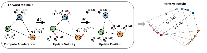
Figure 2: PINGO schematic. The forward step (left box) first uses GNN $f_{\theta}$ (We omit $\theta$ subscript in the figure for brevity) to decide second-order derivatives of particles and then updates their velocities and positions in order. The right part is the trajectory obtained by iteratively repeating the forward process in a 3-body system.

Since $\bm{q}^{(t)}_{\theta}$ is computed through discrete numerical integration, optimizing Eq. 7 will not yield a neural network that can perfectly reconstruct the true $\bm{q}^{(t)}$, even if the loss is zero. Existing theoretical findings [37] illustrate that training using discrete integration trajectories results in a bounded approximation of their first-order derivative, where the bound is linked to the chosen timestep. Given $\mathcal{B}(\bm{q},r)\subset\mathbb{C}^{3}$ as the complex ball of radius $r>0$ centered at $\bm{q}\in\mathbb{C}^{3}$, and time interval $T=t_{1}-t_{0}$, the following holds:

Theorem 4.2.

Let $\bm{q}_{1},\bm{q}_{2}\in\mathbf{R}^{3}$ and $r_{1},r_{2}>0$, the ODE solver is Euler solver and it iterates $\tau$ times with timestep $\Delta t$. Suppose that the target $f$ and the learned $f_{\theta}$ are analytic and bounded by $m_{2}$ on $\mathcal{B}(\bm{q}_{2},r_{2})$, and the target $g$ and the learned $g_{\theta}$ are analytic and bounded by $m_{1}$ on $\mathcal{B}(\bm{q}_{1},r_{1})$. Then, there exist constants $T_{0}$ such that, if $0<T<T_{0}$,

$$||f_{\theta}(\bm{q},\bm{h})-f(\bm{q},\bm{h})||_{\infty}\leq O(\Delta t+\frac{\mathcal{L}}{\Delta t}),\quad\forall\bm{q}\in\mathbf{R}^{3},$$

where $\mathcal{L}=\frac{1}{T}||\bm{q}^{(t_{1})}_{\theta}-\bm{q}^{(t_{1})}||_{\infty}$ represents prediction error in $l_{\infty}$ - norm.

The proof is reported in the Appendix. Based on Theorem 4.2, we analyze the error introduced by the Euler solver. We use two metrics common in classical numerical analysis, namely, local and global truncation error. The local truncation error $\epsilon_{t+\Delta t}$ of PINGO is defined as follows:

$$\epsilon_{t+\Delta t}=||\bm{q}^{(t+\Delta t)}-\bm{q}^{(t)}-\bm{\dot{q}}^{(t)}\Delta t-f_{\theta}(\bm{q}^{(t)},\bm{h})\Delta t^{2}||_{2},$$ (10)

which represents the error accumulated in a single step. And the global truncation error $\mathcal{E}_{t+k\Delta t}$ is defined as follows:

$$\mathcal{E}_{t+k\Delta t}=||\bm{q}^{(t+k\Delta t)}-\bm{q}^{(t+k\Delta t)}_{\theta}||_{2},$$ (11)

which denotes the error accumulated in the first k steps. Then we have

Corollary 4.3.

Given the same conditions as in Theorem 4.2, if the training loss $L$ is adequately minimized and $g_{\theta}$ satisfies the Lipschitz condition, the local truncation error $\epsilon_{t+\Delta t}$ and the global truncation error $\mathcal{E}_{t+k\Delta t}$ are $O(\Delta t^{2})$ and $O(\Delta t)$, respectively.

The proof is reported in Appendix. Corollary 4.3 shows that for the prediction of $\tau$-th iteration, its error depends on the chosen $\Delta t$. These statements imply that PINGO can be trained by minimizing Eq. 7 and generalize to other timesteps.

4.3 Equivariance of PINGO

Given particle positions at time $t$, computing the resultant force of each body is the key to modeling its dynamic changes. In general, PINGO is flexible and can incorporate various GNNs as the backbone, among which equivariant graph neural networks have shown effectiveness in preserving the symmetry of physical systems. For example, if we rotate the input system, the model output will be rotated to the same degree as well. There exist multiple symmetry groups for 3-dimensional systems such as SO(3) (i.e., rotational equivariance) and SE(3) (i.e., rotational and translational equivariance). We can prove that PINGO would not break the equivariance property of backbone GNNs.

Proposition 4.4.

Suppose the backbone GNN $f_{\theta}$ of PINGO is equivariant to group $\mathcal{G}$, then the trajectory $\bm{q}_{\theta}$ is equivariant to group $\mathcal{G}$.

The proof and detailed discussion of equivariance is provided in Appendix. Intuitively, the integration step Eq. 8 only involves the linear computation of equivariant terms, thus PINGO would preserve the same equivariant property as the used GNNs. Specifically, we choose the widely used EGNN [28] as the example of backbone, assuming the acceleration depends on positions, the message passing is defined by

$$\begin{gathered}\bm{m_{ij}}=\phi_{e}\left(||\bm{q}_{\theta,i}-\bm{q}_{\theta,j}||^{2},\bm{h}_{i},\bm{h}_{j},a_{ij}\right),\quad\bm{\ddot{q}}_{\theta,i}=\frac{1}{N-1}\sum_{j\in\mathcal{N}_{i}}(\bm{q}_{\theta,i}-\bm{q}_{\theta,j})\phi_{q}(\bm{m}_{ij}).\\ \bm{h}_{i}^{(t+\Delta t)}=\bm{h}_{i}^{(t)}+\phi_{h}\left(\bm{h}_{i}^{(t)},\sum_{j\in\mathcal{N}_{i}}\bm{m_{ij}}\right).\end{gathered}$$ (12)

Here $\phi_{e},\phi_{x}$ denotes Multi-Layer Perceptrons (MLP) whose output is a scalar and the output of $\phi_{h}$ is a vector. The non-geometric features are updated via skip connections. Analogous to neural ODE methods, the model parameters are shared among all iterations.

5 Experiments

5.1 N-body system

We build upon the experimental setting introduced in [28] where the task is to estimate all particle positions after a fixed timestep. We consider two types of N-body systems, charged and gravity particles, which are driven by electromagnetic [21] and gravitational forces [3] between every pair of particles respectively. Each system consists of 5 particles that have initial position, velocity, and attributes like positive/negative charge or mass. We sample 3000 trajectories for training, 2000 for validation, and 2000 for testing.

Implementation details

We compare our method with GNN and equivariant methods: Radial Field [22], TFN [31], SE(3) Transformer [9], EGNN[28], GMN [15], and SEGNN [3]. In addition, we also compare to Graph Neural Ordinary Differential Equation (GDE) [25]. Without specification, we use EGNN as the backbone of PINGO. The layer number is searched within 10. All algorithms are trained under the same conditions, 100 batch size, 1000 epochs, and Adam optimizer [20]. The learning rate is tuned independently for each model for the best performance. The size of hidden layers is set to 64. Following the setting of existing works [28, 15], linear mapping of the initial velocity norm is provided as input node features for baselines.

Table 1: Mean squared error ($\times 10^{-2}$) of the N-body system, and forward time in seconds for a batch size of 100 samples on Tesla T4 GPU. The header of each column is the time step for training and prediction. Bold font indicates the best result and Underline is the strongest baseline. Results are averaged across 5 runs. We report both mean and standard deviation in the table.

Method	Charged			Gravity			Time [s]
	1000 ts	1500 ts	2000 ts	1000 ts	1500 ts	2000 ts
Linear	6.830$\pm$ 0.016	20.012$\pm$ 0.029	39.513$\pm$ 0.061	7.928$\pm$ 0.001	29.270$\pm$ 0.003	58.521$\pm$ 0.003	0.0002
GNN	1.077$\pm$ 0.004	5.059$\pm$ 0.250	10.591$\pm$ 0.352	1.400$\pm$ 0.071	4.691$\pm$ 0.288	10.508$\pm$ 0.432	0.0064
GDE	1.285$\pm$ 0.074	4.026$\pm$ 0.164	8.708$\pm$ 0.145	1.412$\pm$ 0.095	2.793$\pm$ 0.083	6.291$\pm$ 0.153	0.0088
TFN	1.544$\pm$ 0.231	11.116$\pm$ 2.825	23.823$\pm$ 3.048	3.536$\pm$ 0.067	37.705$\pm$ 0.298	73.472$\pm$ 0.661	0.0440
SE(3)-Tr.	2.483$\pm$ 0.099	18.891$\pm$ 0.287	36.730$\pm$ 0.381	4.401$\pm$ 0.095	52.134$\pm$ 0.898	98.243$\pm$ 0.647	0.2661
Radial Field	1.060$\pm$ 0.007	12.514$\pm$ 0.089	26.388$\pm$ 0.331	1.860$\pm$ 0.075	7.021$\pm$ 0.150	16.474$\pm$ 0.033	0.0052
EGNN	0.711$\pm$ 0.029	2.998$\pm$ 0.089	6.836$\pm$ 0.093	0.766$\pm$ 0.011	3.661$\pm$ 0.055	9.039$\pm$ 0.216	0.0126
GMN	0.824$\pm$ 0.032	3.436$\pm$ 0.156	7.409$\pm$ 0.214	0.620$\pm$ 0.043	2.801$\pm$ 0.194	6.756$\pm$ 0.427	0.0137
SEGNN	0.448$\pm$ 0.003	2.573$\pm$ 0.053	5.972$\pm$ 0.168	0.471$\pm$ 0.026	2.110$\pm$ 0.044	5.819$\pm$ 0.335	0.0315
PINGO	0.433$\pm$ 0.013	2.183$\pm$ 0.048	5.614$\pm$ 0.126	0.338$\pm$ 0.027	1.693$\pm$ 0.217	4.857$\pm$ 0.760	0.0277

Table 2: The generalization from long-term to short-term. All models are trained on 1000ts and test on 250/500/750/1000 ts. Mean squared error ($\times 10^{-2}$) and the standard deviation are reported. Results averaged across 5 runs.

Method	Charged					Gravity
	$250$ ts	$500$ ts	$750$ ts	$1000$ ts	Avg	$250$ ts	$500$ ts	$750$ ts	$1000$ ts	Avg
GNN	73.40$\pm$9.60	31.79$\pm$5.28	12.86$\pm$2.81	0.826$\pm$0.08	29.72	181.9$\pm$26.1	90.33$\pm$15.5	30.66$\pm$12.3	0.746$\pm$0.05	75.93
GDE	92.65$\pm$25.0	43.94$\pm$10.9	12.20$\pm$23.2	0.652$\pm$0.05	37.36	136.0$\pm$135	56.80$\pm$60.6	12.21$\pm$14.8	0.588$\pm$0.58	51.39
EGNN	6.756$\pm$3.05	3.816$\pm$4.68	3.668$\pm$0.74	0.568$\pm$0.09	3.702	7.146$\pm$7.06	29.70$\pm$20.4	9.712$\pm$3.60	0.382$\pm$0.11	11.89
GMN	10.44$\pm$7.43	10.92$\pm$4.67	4.518$\pm$1.36	0.512$\pm$0.16	6.598	7.430$\pm$8.19	9.540$\pm$12.1	5.730$\pm$6.69	0.349$\pm$0.48	5.762
SEGNN	21.78$\pm$9.69	52.74$\pm$15.6	34.13$\pm$14.9	0.342$\pm$0.04	27.25	10.58$\pm$6.28	49.63$\pm$37.7	25.82$\pm$27.0	0.448$\pm$0.02	21.62
PINGO	0.188$\pm$0.03	0.312$\pm$0.06	0.360$\pm$0.06	0.309$\pm$0.11	0.292	0.064$\pm$0.02	0.128$\pm$0.03	0.176$\pm$0.04	0.210$\pm$0.07	0.145

Results on the direct prediction.

Table 4 depicts the overall results of the direct prediction results on two datasets. For each dataset, besides the common setting with 1000 time step (1000 ts), we add two additional settings (1500 ts and 2000 ts) to evaluate the performance of long-term prediction. Meanwhile, we report the average forward time in seconds for 100 samples of each method. From Table 4 we can observe that:

• It is evident that PINGO, equipped solely with EGNN, outperforms all baselines across all datasets and settings. Notably, compared to the best baseline SEGNN, the average error improvement on Charged and Gravity datasets is $0.254$ and $0.504$ respectively, indicating significant improvement.

• As the time step increases, PINGO’s performance improvement becomes more pronounced. Compared to the best baseline SEGNN, the average error improvement increases from $0.074$ at 1000 time steps to $0.660$ at 2000 time steps, demonstrating the efficacy of PINGO in handling long-term prediction scenarios.

• As expected, PINGO’s forward time ($0.0277$s) is slower than that of EGNN ($0.0126$s) due to its additional integration operation. Nevertheless, PINGO’s forward time remains competitive compared to the best baselines ($0.0315$), indicating its efficiency.

Generalization capability from long-term to short-term.

It is interesting to see how PINGO can generalize from long-term training to short-term testing. Accordingly, we train models on 1000ts on two datasets and make the test on shorter time steps by performing PINGO on the smaller $\tau$ step with the same ratio. For the baselines, we extract the object position information from their hidden layers as the prediction of its intermediate steps. Table 2 reports the mean and standard deviation of each setting. From Table 2 we can observe that:

• Clearly, PINGO outperforms all other baselines across all settings by a large margin. Notably, when there is a lack of supervised signals at 250/500/750ts, the performance of all other baselines decreases significantly. By contrast, PINGO achieves similar results as in 1000ts, demonstrating its robust generalization to short-term prediction.

• Another interesting point is that PINGO’s error exhibits a distinct trend compared to other baselines. While the errors of other baselines significantly increase with decreasing time steps, PINGO achieves even smaller errors with shorter time steps. This observation justifies our theoretical results that the error is bound by the chosen timestep.

• Additionally, the standard deviation of PINGO is much smaller than that of other baselines, indicating the numerical stability of PINGO. This result further confirms our theoretical finding that PINGO can obtain the unique latent trajectory between two discrete states.

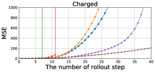
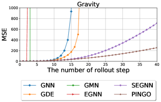
Figure 3: Mean squared error for the long-term simulation by rollout. All models are trained on 1000ts.

Generalization capability for the long-term simulation.

In this part, we evaluate the generalizability of models for extreme long-term simulation. Specifically, we train all models on 1000ts and use rollout to make the prediction for the longer time step (over 40 rollout steps, indicating over 40000ts.). Figure 3 depicts the mean squared error of all methods on two datasets. As shown in Figure 3, all baselines experience numerical explosion due to error accumulation during the rollout process, leading to a quick drop in prediction performance. In contrast, PINGO demonstrates an order-of-magnitude error improvement over other baselines for the extreme long-term simulation. This numerical stability can be attributed to the Neural ODE framework for modeling position and velocity. Nevertheless, we also noticed an increase in errors during the rollout process in PINGO. We conjecture this error may be introduced by the incorrect force estimation by GNN. Therefore, a more powerful GNN with better force estimation ability could further enhance the performance of PINGO.

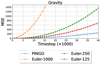
Figure 4: Mean squared error for PINGO and symplectic Euler solver on the gravity system, which is calculated between them and groundtruth (i.e., Euler-1).

Compared with numerical methods

To verify the effectiveness of PINGO, we further compare it with symplectic Euler solvers that have a closed-form solution. The results of the gravity system are illustrated in Figure 4, and we provide results of charged systems in Appendix. Euler-$\Delta t$ denotes results using $\Delta t$ as the forward timestep. From the figure, we can find that under the same timestep (i.e., Euler-125), PINGO achieves better long-term performance. According to Corollary 4.3, PINGO is at least a first-order method if the prediction error is adequately minimized. Since the timestep of PINGO is set to 125, under appropriate conditions, PINGO will at least achieve comparable performance with Euler-125.

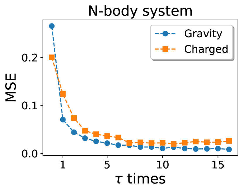
Figure 5: Effects of iteration times $\tau$.

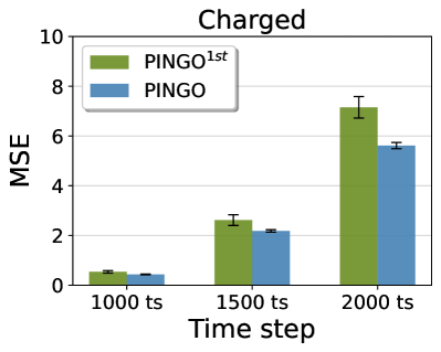
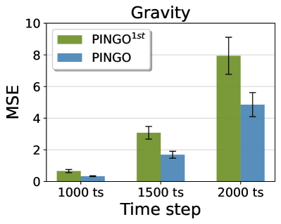
Figure 6: Comparison between PINGO and PINGO^1st, which is a PINGO variant modeling the first-order derivatives of positions.

Ablation study

We conduct two ablation studies on PINGO: (1) To validate the effectiveness of second-order modeling, we compare PINGO with its first-order variant PINGO^1st, where we use the same backbone and experimental settings to learn the first-order derivatives. The results are shown in Figure 6, we can observe that PINGO consistently enhances performance across all scenarios, with particularly notable improvements in long-term simulations. This validates the efficacy of incorporating second-order derivatives in modeling physical systems, emphasizing the significant advantages of integrating physical knowledge into the learning of dynamical systems; (2) Then we study the effect of the chosen timestep via increasing the iteration times $\tau$. Since the target timestep is fixed, a larger iteration time indicates a smaller timestep. The results are displayed in Figure 6. It is obvious that better results can be achieved by choosing a small timestep. Additionally, the performance would not increase after a sufficient iteration, which is around 10 in both datasets. According to Theorem 4.2, these errors are mainly attributed to learning loss which is related to the representative ability of GNNs.

5.2 CMU Motion Capture

For real-world applications, we evaluate our model on CMU Motion Capture Databse [5], which contains various trajectories of human motions. Our main focus lies in the walking motion of a single object (subject #35) [21]. We adopt a random split strategy introduced by [15] where train/validation/test data contains 200/600/600 frame pairs. For comprehensive evaluations of long-term performance, we broaden our assessment scope to include scenarios with intervals of 40 ts and 50 ts, in addition to the default settings with 30 ts.

Implementation details

In this task, we use GMN as the backbone of PINGO. The norm of velocity and the coordinates of the gravity axis (z-axis) are set as node features to represent the motion dynamics. Note that the human body operates through joint interactions, we augment the edges with 2-hop neighbors. These operations are implemented across all applicable baselines. Following [15], 6 key bones are selected as sticks and the rest are isolated objects for GMN configurations.

Results

Table 3 reports the performance of PINGO and various compared models. It is evident that PINGO outperforms all baseline models by a significant margin across all scenarios. Notably, the improvements are more pronounced in long-term simulations, with PINGO achieving 18.619 $\times$ 10^-2 lower MSE than the runner-up model GMN. To gain further insights into the superior performance of PINGO, we illustrate the predicted motion of GMN and PINGO in Figure 7. Interestingly, it can be observed that the predictions of GMN appear to lag behind the ground truths, while PINGO demonstrates a closer match. This discrepancy may be attributed to the lack of constraints imposed by modeling the rollout trajectories. We provide more visualizations in Appendix.

Table 3: Mean squared error ($\times 10^{-2}$) on CMU motion capture dataset. Results are averaged across 5 runs.

Model	TFN	SE(3)-Tr.	RF	EGNN	GMN	PINGO	Abs. Imp.
$30$ ts	24.932$\pm$ 1.023	24.655$\pm$ 0.870	149.459$\pm$ 0.750	24.013$\pm$ 0.462	16.005$\pm$ 0.386	14.462$\pm$ 0.106	1.543
$40$ ts	49.976$\pm$ 1.664	44.279$\pm$ 0.355	306.311$\pm$ 1.100	39.792$\pm$ 2.120	38.193$\pm$ 0.697	22.229$\pm$ 1.489	15.964
$50$ ts	73.716$\pm$ 4.343	68.796$\pm$ 1.159	549.476$\pm$ 3.461	50.930$\pm$ 2.675	47.883$\pm$ 0.599	29.264$\pm$ 0.946	18.619

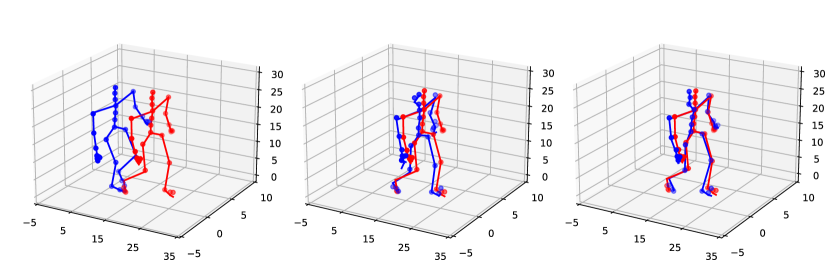
Figure 7: Visualization of Motion Capture with 50 time step. Left to Right: initial position, GMN, PINGO (all in blue). Ground truths are in red.

6 Conclusions

In this work, we highlight the problem of long-term simulation of N-body systems and introduce PINGO, a flexible neural graph ODE framework that is capable of learning physical dynamics from observed trajectories. Its core idea is to learn latent physical dynamics and employ numerical methods to infer system states. Theoretical findings show that our model can generalize to other timesteps via the same training criteria as existing studies. We demonstrate the potential of PINGO by applying it to a wide range of physical systems. PINGO outperforms all competitors in all cases. Extensive ablation studies have further verified the generalization ability of PINGO and the effectiveness of its physical design.

Appendix A Proofs

Note that $\boldsymbol{h}$ is identical for both authentic and learned systems. Unless otherwise specified, we omit $\boldsymbol{h}$ in the following discussions.

A.1 Proof of Proposition 4.1

Let $\bm{q}^{(t)}=\bm{q}(t),\bm{q}_{\theta}^{(t)}=\bm{q}_{\theta}(t)$ be the dynamic function at time $t$. Recall that $\bm{\dot{q}}^{(t)}=g(\bm{q}^{(t)}),\bm{\ddot{q}}^{(t)}=f(\bm{q}^{(t)})$ and $\bm{\dot{q}}_{\theta}^{(t)}=g_{\theta}(\bm{q}_{\theta}^{(t)}),\bm{\ddot{q}}_{\theta}^{(t)}=f_{\theta}(\bm{q}_{\theta}^{(t)})$ are the first-order and second-order derivatives of $\bm{q}(t),\bm{q}_{\theta}(t)$ respectively. Suppose $\bm{q}(t)$ is not equal to $\bm{q}_{\theta}(t)$ and they both satisfy $\bm{q}^{(t_{0})}=\bm{q}_{\theta}^{(t_{0})}$, $\bm{q}^{(t_{1})}=\bm{q}_{\theta}^{(t_{1})}$, and $\bm{\dot{q}}^{(t_{0})}=\bm{\dot{q}}_{\theta}^{(t_{0})}$, we define

$$\bm{\widetilde{q}}^{(t)}=\bm{q}(t)-\bm{q}_{\theta}(t).$$ (13)

Then we have:

$$\bm{\widetilde{q}}^{(t_{0})}=\bm{q}^{(t_{0})}-\bm{q}_{\theta}^{(t_{0})}=0,\quad\bm{\widetilde{q}}^{(t_{1})}=\bm{q}^{(t_{1})}-\bm{q}_{\theta}^{(t_{1})}=0,\quad\bm{\dot{\widetilde{q}}}^{(t_{1})}=\bm{\dot{q}}^{(t_{1})}-\bm{\dot{q}}_{\theta}^{(t_{1})}=0.$$ (14)

Then based on Picard–Lindelöf theorem [6], assuming $f$ is continuous on $\bm{q}(t)$ and $f_{\theta}$ is continuous on $\bm{q}_{\theta}(t)$, there has a unique solution $\bm{\widetilde{q}}^{(t)}=0,t\in[t_{0},t_{1}]$. Since $\bm{\widetilde{q}}^{(t_{0})}=0$, $\bm{q}(t)=\bm{q}_{\theta}(t)$ and thus $f(\bm{q}^{(t)})=f_{\theta}(\bm{q}^{(t)})$.

A.2 Proof of Theorem 4.2

The proof sketch is as follows: We first introduce the definitions pertaining to neural ODE in PINGO, then derive the bound for first-order approximation error $||g_{\theta}-g||_{\infty}$, and finally extend the results to the second-order case $||f_{\theta}-f||_{\infty}$ to finish the proof.

A.2.1 Neural ODE Solver

As stated in Eq. 7, given the discrete training set $\mathcal{D}_{\text{train}}=\{\bm{q}_{s}^{(t_{0})},\bm{q}_{s}^{(t_{1})}\}_{s=1}^{D}$, the objective of PINGO is to minimize the discrepancy between the exact and approximated positions at time $t_{1}$ via

$$\mathcal{L}_{\text{train}}=\sum_{s\in\mathcal{D}_{\text{train}}}||\bm{q}_{\theta,s}^{(t_{1})}-\bm{q}_{s}^{(t_{1})}||^{2},$$ (15)

where, $\bm{q}_{\theta}^{(t_{1})}\coloneqq\phi_{T,g_{\theta}}(\bm{q}^{(t_{0})})$, $T=t_{1}-t_{0}$ is the prediction given $\bm{q}^{(t_{0})}$ as input. To model the latent continuous trajectory between $t_{0}$ and $t_{1}$, we use the ODE formulation from the dynamic system in Eq. 3 to calculate any position $\bm{q}^{(t_{0}+t^{\prime})}$,$t^{\prime}\in[0,T]$.

$$\phi_{t^{\prime},g}(\bm{q}^{(t_{0})})\coloneqq\bm{q}^{(t_{0})}+\int_{t_{0}}^{t_{0}+t^{\prime}}g(\bm{q}^{(t)})\,dt,$$ (16)

where $g$ represents the mapping from the trajectory to its first-order derivative in a dynamical system. In this vein, we can rewrite $\bm{q}_{s}^{(t_{1})}$ as $\phi_{T,g}(\bm{q}^{(t_{0})})$. Furthermore, we introduce the parameterization trick on the acceleration by Eq. 6 and $\phi_{T,g_{\theta}}(\bm{q}^{(t_{0})})$ can be defined by:

$$\phi_{T,g_{\theta}}(\bm{q}^{(t_{0})})=\bm{q}^{(t_{0})}+\int_{t_{0}}^{t_{0}+T}g_{\theta}(\bm{q}^{(t)})\,dt,$$ (17)

where $g_{\theta}$ is the parameterized version of $g$ determined by $f_{\theta}$ via Eq. 6, 8 and 9. Since it is infeasible to directly obtain the integration $\int_{t_{0}}^{t_{0}+T}g_{\theta}(\bm{q}^{(t)})\,dt$ with parameterized $g_{\theta}$, in PINGO, we utilize the Euler integrator to generate a discrete trajectory that serves as an approximation of the latent continuous trajectory between $t_{0}$ and $t_{1}$. Specifically, we divide the entire time interval $T=t_{1}-t_{0}$ into $\tau$ equal intervals with time step $\Delta t=T/\tau$. The Euler integrator $\Phi_{\Delta t,g}$ approaches $\phi_{\Delta t,g}$ via

$$\Phi_{\Delta t,g}(\bm{q}^{(t_{0})})=\bm{q}^{(t_{0})}+g(\bm{q}^{(t_{0})})\Delta t.$$ (18)

For approximation, PINGO composites $\tau$ Euler integrator $\phi_{\Delta t,g_{\theta}}$ as a neural ODE solver in the following form

$$\bm{q}_{\theta}^{(t_{1})}=\phi_{T,g_{\theta}}(\bm{q}^{(t_{0})})=\Phi_{\Delta t,g_{\theta}}\circ\cdots\circ\Phi_{\Delta t,g_{\theta}}(\bm{q}^{(t_{0})})=(\Phi_{\Delta t,g_{\theta}})^{\tau}(\bm{q}^{(t_{0})}).$$ (19)

Given such, it is straightforward to reframe our learning objective in the context of a neural ODE:

$$\mathcal{L}_{\text{train}}=\sum_{s\in\mathcal{D}_{\text{train}}}||\bm{q}_{\theta,s}^{(t_{1})}-\bm{q}_{s}^{(t_{1})}||^{2}=\sum_{s\in\mathcal{D}_{\text{train}}}||(\Phi_{\Delta t,g_{\theta}})^{\tau}(\bm{q}^{(t_{0})}_{s})-\phi_{T,g}(\bm{q}^{(t_{0})}_{s})||^{2}.$$ (20)

A.2.2 Approximation Error of $f_{\theta}$

In our dynamical system, $g_{\theta}$ and $g$ are entirely determined by $f_{\theta}$ and $f$ respectively. Thus, we first establish the boundedness of $||g_{\theta}-g||_{\infty}$, then demonstrate the approximation error of $||f_{\theta}-f||_{\infty}$.

Lemma A.1.

For $\bm{q}_{0}\in\mathbb{R}^{3}$ and $r_{a}$, $r_{b}>0$, a given ODE solver that is $\tau$ compositions of an Euler Integrator $\Phi_{\Delta t,g_{\theta}}$ with $\Delta t=T/\tau$, let

$$\mathcal{L}=\frac{1}{T}||(\Phi_{\Delta t,g_{\theta}})^{\tau}(\bm{q}_{0})-\phi_{T,g}(\bm{q}_{0})||_{\infty},$$ (21)

and suppose that $g$ and $g_{\theta}$ are analytic and bounded by $m$ within $\mathcal{B}(\bm{q}_{0},r_{a}+r_{b})$, a complex ball centered at $\bm{q}_{0}$ with radius $r_{a}+r_{b}$. Then, there exist constants $T_{0}$ and $C$ that depends on $r_{a}/m$, $r_{b}/m$, $\tau$, and $\Phi_{\Delta t,g_{\theta}}$, such that, if $0<T<T_{0}$,

$$||g_{\theta}(\bm{q})-g(\bm{q})||_{\infty}\leq Cm\Delta t+\frac{e}{e-1}\mathcal{L},\quad\,\forall\bm{q}\in\mathbb{R}^{3},$$ (22)

where $e$ is the base of the natural logarithm.

Proof.

This result can be directly derived from Theorem 3.1 and 3.2 in [37] via replacing the integrator from Runge-Kutta integrator with Euler integrator since Euler integrator has been proven to satisfy the prerequisites of theorems in Appendix B.2 in [37]. ∎

From our assumption, let $\bm{q}_{1}=\bm{q}^{(t_{0})}$, then $g$ and $g_{\theta}$ are both analytic and bounded by $m_{1}$ in $\mathcal{B}(\bm{q}^{(t_{0})},r_{1})$. By utilizing Lemma A.1, where we set $\bm{q}_{0}=\bm{q}^{(t_{0})}$ and $T<T_{0}$, we can derive that

$$||g_{\theta}(\bm{q})-g(\bm{q})||_{\infty}\leq C_{1}m_{1}\Delta t+\frac{e}{e-1}\mathcal{L},\quad\,\forall\bm{q}\in\mathbb{R}^{3},$$ (23)

where $\mathcal{L}=\frac{1}{T}||\bm{q}^{(t_{1})}_{\theta}-\bm{q}^{(t_{1})}||_{\infty}$ and $C_{1}$ is a control constant.

To establish the connection between $g$ and $f$, we only focus on the first time step $\Delta t$ instead of the entire time interval $T$. Note that $g$ is obtained by integrating $f$, we denote

$$\psi_{\Delta t,g,f}(\bm{q}^{(t_{0})})\coloneqq g(\bm{q}^{(t_{0}+\Delta t)})=g(\bm{q}^{(t_{0})})+\int_{t_{0}}^{t_{0}+\Delta t}f(\bm{q}^{(m)})\,dm,$$ (24)

as the flow map for the first-order derivative of the exact trajectory in a single step. Analogously, its corresponding Euler integrator is defined as

$$\Psi_{\Delta t,g,f}(\bm{q}^{(t_{0})})=g(\bm{q}^{(t_{0})})+f(\bm{q}^{(t_{0})})\Delta t.$$ (25)

With our iterative update scheme in Eq. 8, we denote

$$g_{\theta}(\bm{q}^{(t_{0}+\Delta t)}_{\theta})=\Psi_{\Delta t,g_{\theta},f_{\theta}}(\bm{q}^{(t_{0})}),$$ (26)

as a neural ODE solver for $\psi_{\Delta t,g,f}(\bm{q}^{(t_{0})})$. In the meantime, PINGO produces

$$\bm{q}_{\theta}^{(t_{0}+\Delta t)} =\bm{q}^{(t_{0})}+g_{\theta}(\bm{q}_{\theta}^{(t_{0}+\Delta t)})\Delta t$$ (27)

$$=\bm{q}^{(t_{0})}+g(\bm{q}^{(t_{0})})\Delta t+f_{\theta}(\bm{q}^{(t_{0})})\Delta t^{2},$$

as the estimation of discretized trajectory for the first time step. Then, with suitable $\Delta t$ and $r_{1}$ , $g_{\theta}(\bm{q}_{\theta}^{(t_{0}+\Delta t)})$ is bounded since $\bm{q}_{\theta}^{(t_{0}+\Delta t)}\in\mathcal{B}(\bm{q}^{(t_{0})},r_{1})$.

Note that $f$ and $f_{\theta}$ are both analytic and bounded by $m_{2}$ in $\mathcal{B}(\bm{q}_{2},r_{2})$. In lemma A.1, we substitute $\phi_{\Delta t,g_{\theta}}$ by $\Psi_{\Delta t,g_{\theta},f_{\theta}}$ and set $T=\Delta t$ with $\tau=1$, then the corresponding loss becomes

$$\mathcal{L}_{1} =\frac{1}{\Delta t}||\Psi_{\Delta t,g_{\theta},f_{\theta}}(\bm{q}^{(t_{0})})-\psi_{\Delta t,g,f}(\bm{q}^{(t_{0})})||_{\infty}$$ (28)

$$=\frac{1}{\Delta t}||g_{\theta}(\bm{q}^{(t_{0}+\Delta t)}_{\theta})-g(\bm{q}^{(t_{0}+\Delta t)})||_{\infty}$$

$$=\frac{1}{\Delta t}||g_{\theta}(\bm{q}^{(t_{0}+\Delta t)}_{\theta})-g_{\theta}(\bm{q}^{(t_{0}+\Delta t)})+g_{\theta}(\bm{q}^{(t_{0}+\Delta t)})-g(\bm{q}^{(t_{0}+\Delta t)})||_{\infty}$$

$$\leq\frac{1}{\Delta t}(2m_{1}+C_{1}m_{1}\Delta t+\frac{e}{e-1}\mathcal{L}).$$

Subsequently, given that $\Delta t<T<T_{0}$, we have

$$||f_{\theta}(\bm{q})-f(\bm{q})||_{\infty} \leq C_{2}m_{2}\Delta t+\frac{e}{e-1}\mathcal{L}_{1},$$ (29)

$$\leq C_{2}m_{2}\Delta t+\frac{e}{e-1}\big{[}\frac{1}{\Delta t}(2m_{1}+C_{1}m_{1}\Delta t+\frac{e}{e-1}\mathcal{L})\big{]},$$

$$\leq C_{2}m_{2}\Delta t+(\frac{e}{e-1})^{2}\frac{\mathcal{L}}{\Delta t}+\frac{e}{e-1}(\frac{2m_{1}}{\Delta t}+C_{1}m_{1}),$$

$$\leq O(\Delta t+\frac{\mathcal{L}}{\Delta t}),\quad\forall\,\bm{q}\in\mathbb{R}^{3},$$

which concludes the proof.

A.3 Proof of Corollary 4.3

A.3.1 Local truncation error

We use Taylor series expansion to approximate the trajectory at time $t+\Delta t$:

$$\bm{q}^{(t+\Delta t)}=\bm{q}^{(t)}+g(\bm{q}^{(t)})\Delta t+\frac{1}{2}f(\bm{q}^{(t)})\Delta t^{2}+O(\Delta t^{3}).$$ (30)

Then the local truncation error $\epsilon_{t+\Delta t}$ equals to:

$$\epsilon_{t+\Delta t} =||\bm{q}^{(t+\Delta t)}-\bm{q}^{(t)}-g(\bm{q}^{(t)})\Delta t-f_{\theta}(\bm{q}^{(t)})\Delta t^{2}||_{2}$$ (31)

$$=||\bm{q}^{(t)}+g(\bm{q}^{(t)})\Delta t+\frac{1}{2}f(\bm{q}^{(t)})\Delta t^{2}+O(\Delta t^{3})-\bm{q}^{(t)}-g(\bm{q}^{(t)})\Delta t-f_{\theta}(\bm{q}^{(t)})\Delta t^{2}||_{2}$$

$$=||\frac{1}{2}f(\bm{q}^{(t)})\Delta t^{2}-f_{\theta}(\bm{q}^{(t)})\Delta t^{2}+O(\Delta t^{3})||_{2}$$

$$=||\frac{1}{2}(f(\bm{q}^{(t)})-f_{\theta}(\bm{q}^{(t)}))\Delta t^{2}-\frac{1}{2}f_{\theta}(\bm{q}^{(t)})\Delta t^{2}+O(\Delta t^{3})||_{2}$$

$$\leq||\frac{1}{2}(f(\bm{q}^{(t)})-f_{\theta}(\bm{q}^{(t)}))\Delta t^{2}||_{2}+||\frac{1}{2}f_{\theta}(\bm{q}^{(t)})\Delta t^{2}||_{2}+O(\Delta t^{3})$$

$$\leq\frac{\sqrt{3}\Delta t^{2}}{2}||f(\bm{q}^{(t)})-f_{\theta}(\bm{q}^{(t)}))||_{\infty}+||\frac{1}{2}m_{2}\Delta t^{2}||_{2}+O(\Delta t^{3})$$

$$\leq\frac{\sqrt{3}\Delta t^{2}}{2}O(\Delta t+\frac{\mathcal{L}}{\Delta t})+O(\Delta t^{2}).$$

Here the last inequality is due to Theorem 4.2. If loss $\mathcal{L}$ is sufficiently small, then the last term $\frac{\sqrt{3}\Delta t^{2}}{2}O(\Delta t+\frac{\mathcal{L}}{\Delta t})+O(\Delta t^{2})$ is $O(\Delta t^{2})$.

A.3.2 Global truncation error

The bound on the global truncation error can be derived on a recursive way:

$$\mathcal{E}_{t+(k+1)\Delta t} =\bm{q}^{(t+(k+1)\Delta t)}-\bm{q}^{(t+(k+1)\Delta t)}_{\theta}$$ (32)

$$=\bm{q}^{(t+(k+1)\Delta t)}-\bm{q}^{(t+k\Delta t)}_{\theta}-g_{\theta}(\bm{q}_{\theta}^{(t+k\Delta t)})\Delta t$$

$$=\bm{q}^{(t+k\Delta t)}-\bm{q}^{(t+k\Delta t)}_{\theta}+\bm{q}^{(t+(k+1)\Delta t)}-\bm{q}^{(t+k\Delta t)}-g(\bm{q}^{(t+k\Delta t)})\Delta t$$

$$\quad+g_{\theta}(\bm{q}^{(t+k\Delta t)})\Delta t-g_{\theta}(\bm{q}_{\theta}^{(t+k\Delta t)})\Delta t$$

$$=\mathcal{E}_{t+k\Delta t}+\epsilon_{t+(k+1)\Delta t}+(g_{\theta}(\bm{q}^{(t+k\Delta t)})-g_{\theta}(\bm{q}_{\theta}^{(t+k\Delta t)}))\Delta t.$$

Note that $g_{\theta}$ satisfies the Lipschitz condition, we have:

$$||g_{\theta}(\bm{q}^{(t+k\Delta t)})-g_{\theta}(\bm{q}_{\theta}^{(t+k\Delta t)})||_{2}\leq L||\bm{q}^{(t+k\Delta t)}-\bm{q}_{\theta}^{(t+k\Delta t)}||_{2}=L||\mathcal{E}_{t+k\Delta t}||_{2},$$ (33)

where $L$ denotes Lipschitz constant for $g_{\theta}$. Thus,

$$||\mathcal{E}_{t+(k+1)\Delta t}||_{2} =||\mathcal{E}_{t+k\Delta t}+\epsilon_{t+(k+1)\Delta t}+(g_{\theta}(\bm{q}^{(t+k\Delta t)})-g_{\theta}(\bm{q}_{\theta}^{(t+k\Delta t)}))\Delta t||_{2}$$ (34)

$$\leq(1+L\Delta t)||\mathcal{E}_{t+k\Delta t}||_{2}+O(\Delta t^{2}).$$

Since the global truncation error $||\mathcal{E}_{t+\Delta t}||_{2}$ at time $t+\Delta t$ is exactly the local truncation error. We have

$$||\mathcal{E}_{t+k\Delta t}||_{2} \leq(1+L\Delta t)^{k-1}O(\Delta t^{2})+\dots+(1+L\Delta t)O(\Delta t^{2})+O(\Delta t^{2})$$ (35)

$$=\frac{(1+L\Delta t)^{k}-1}{(1+L\Delta t)-1}O(\Delta t^{2})=\frac{(1+L\Delta t)^{k}-1}{L\Delta t}O(\Delta t^{2})=O(\Delta t).$$

A.4 Proof of Proposition 4.4

Assume that $a\in\mathcal{G}$ from a group $\mathcal{G}$ is a set of transformations on $\bm{Q}\subseteq\mathbb{R}^{n}$ and function $f:\bm{Q}\rightarrow\bm{Q}$ is a function mapping. Then, we say $f$ is equivariant to transformation $a$ when

$$f(a\circ\bm{q})=a\circ f(\bm{q}),\quad\forall\bm{q}\in\bm{Q}.$$ (36)

Since the backbone GNNs, including EGNN [28], SEGNN [3], and GMN [15], consider the group of rotations, translations, and reflections. Here, we prove that if the GNN $f_{\theta}(\bm{q},\bm{h})$ is translation equivariant on $\bm{q}$ for any translation vector $\bm{b}\in\mathbb{R}^{3}$ and it is rotation and reflection equivariant on $\bm{q}$ for any orthogonal matrix $\bm{Q}\in\mathbb{R}^{3\times 3}$, then PINGO is also translation equivariant on $\bm{q}$ for $\bm{b}$, rotation and reflection equivariant on $\bm{q}$ for $\bm{Q}$. Generally, suppose $f_{\theta}(\bm{q},\bm{h})$ can be divided into a translation-invariant term $f^{\prime}_{\theta}(\bm{q},\bm{h})$ and a translation-equivariant term $\bm{q}$, in each iteration, PINGO computes

$$\bm{q}^{(t+\Delta t)}=\bm{q}^{(t)}+\dot{\bm{q}}^{(t)}\Delta t+f^{\prime}_{\theta}(\bm{q}^{(t)},\bm{h})\Delta t^{2}.$$ (37)

PINGO should satisfy:

$$\bm{Q}\bm{q}^{(t+\Delta t)}+\bm{b}=\bm{Q}\bm{q}^{(t)}+\bm{b}+\bm{Q}\bm{\dot{q}}^{(t)}\Delta t+f^{\prime}_{\theta}(\bm{Q}\bm{q}^{(t)}+\bm{b},\bm{h})\Delta t^{2}.$$ (38)

It is straightforward to show that the above iteration term is equivariant,

$$\bm{Q}\bm{q}^{(t)}+\bm{b}+\bm{Q}\bm{\dot{q}}^{(t)}\Delta t+f^{\prime}_{\theta}(\bm{Q}\bm{q}^{(t)}+\bm{b},\bm{h})\Delta t^{2} =\bm{Q}\bm{q}^{(t)}+\bm{b}+\bm{Q}\bm{\dot{q}}^{(t)}\Delta t+\bm{Q}f^{\prime}_{\theta}(\bm{q}^{(t)},\bm{h})\Delta t^{2}$$ (39)

$$=\bm{Q}(\bm{q}^{(t)}+\bm{\dot{q}}^{(t)}\Delta t+f^{\prime}_{\theta}(\bm{q}^{(t)},\bm{h})\Delta t^{2})+\bm{b}$$

$$=\bm{Q}\bm{q}^{(t+\Delta t)}+\bm{b}$$

Appendix B Experiment details

B.1 N-body system dataset

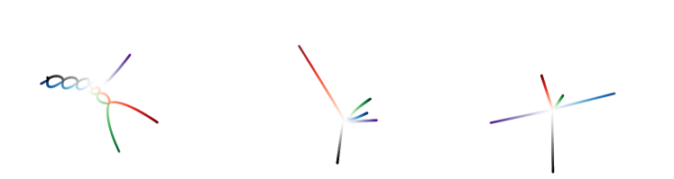
Figure 8: Example trajectories of 5-body charged system. From left to right, the number of positive and negative charges are 1, 3, 0.

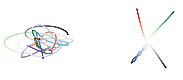
Figure 9: Example trajectories of 5-body gravity system. The system formed by gravitational force can either aggregate (i.e., left) or disperse (i.e., right).

N-body charged system

We use the same N-body charged system code with previous work [28, 3]. They inherit the 2D implementation of  [21] and extend it to 3 dimensions. System trajectories are generated in 0.001 timestep and unbounded with virtual boxes. The initial location is sampled from a Gaussian distribution (mean $\mu=0$, standard deviation $\sigma=0.5$), and the initial velocity is a random vector of norm $0.5$. For comparison in 1000 timestep, to ensure it is consistent with previous work [28, 3], we employ the same generation process with them as shown in the code. We further generate trajectories of duration 45000 timesteps to compare the long-term simulation performance of models. According to the charge types, three types of systems exist where the difference between the number of positive and negative charges are 1, 3, and 0. Example trajectories of these three types of systems are provided in Figure 8.

N-body gravity system

The code of gravitational N-body systems is provided by [3]. They implement it under the same framework as the above charged N-body systems. System trajectories are generated in 0.001 timestep, use gravitational interaction, no boundary conditions. Particle positions are initialized from a unit Gaussian, particle velocities are initialized with a norm equal to one, random direction, and particle mass is set to one. We generate trajectories of duration 45000 timesteps based on the code. The system formed by gravitational force can either aggregate or disperse. Example trajectories of these two types of systems are provided in Figure 9.

B.2 Implementation details

Hyper-parameter

For GNN, GDE, EGNN, GMN, and SEGNN, we empirically find that the following hyper-parameters generally work well, and use them across most experimental evaluations: Adam optimizer with learning rate 0.0005, hidden dim 64, weight decay $1\times 10^{-10}$ and the layer number 4. We set the layer number of PINGO to 8. For N-body systems, the representation degrees of SE(3)-transformer and TFN are set to 3 and 2 respectively. For CMU Motion Capture, all models are trained 3000 epochs using 100 batch size. The representation degrees of SE(3)-transformer and TFN are set to 3 and their learning rate is 0.001 with weight decay $1\times 10^{-8}$. The hyper-parameters of other models are the same as N-body systems.

Long-term simulation

When using rollout to make long-term predictions, dynamic models have to iteratively update the position and velocity. At the time $t_{k}$, if the model jointly outputs the position and velocity, including EGNN, GMN, and PINGO, we use them as the input of prediction at the next timestep. Otherwise, if the model only outputs the position, including GNN, GDE, and SEGNN, we use $\frac{\bm{q}_{\theta}^{(t_{k})}-\bm{q}_{\theta}^{(t_{k-1})}}{t_{k}-t_{k-1}}$ as the velocity input of the prediction at the next timestep.

Appendix C Additional Experiments

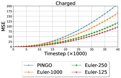
Figure 10: Mean squared error for PINGO and symplectic Euler solver on the charged system. Euler-$\Delta t$ denotes results using $\Delta t$ as the forward timestep.

C.1 Compare PINGO with numerical methods on N-body charged systems

We compare PINGO with the symplectic Euler method, which has closed-form solutions for N-body charged systems, and present the comparison results in Figure 12. Here, PINGO is trained on the supervision at 1000 timesteps with $\Delta t=125$. From Figure 12, we can observe that under the fair setting ($T=1000$), PINGO can achieve better long-term performance than Euler-1000. However, PINGO cannot surpass Euler-125 with a smaller time step ($T=125$). We conjecture that this result is due to the complex dynamic nature of charged systems, which involve both gravitational and repulsive forces, resulting in more diverse dynamics and higher estimate force error by GNN backbones.

C.2 Generalization capability from small systems to large systems

In this part, we evaluate the generalizability of models for larger system sizes. Specifically, we train all models on 5-body gravity systems and then test them on 10-body and 20-body gravity systems. Table 4 shows their results. We compare three strong baselines, i.e., EGNN, GMN, and SEGNN, on modeling 5-body gravity systems. The results show that the performance of all baselines significantly drops when testing on larger systems. In contrast, PINGO still demonstrates a marked improvement over other baselines, especially on 20-body systems. This improvement can be attributed to that PINGO aims to learn the latent dynamics instead of the trajectories themselves.

Table 4: The results on the larger systems. The header of each column shows the number of objects in the system and time step for training and prediction. Mean squared error ($\times 10^{-2}$) and the standard deviation are reported. Bold font indicates the best result and Underline is the strongest baseline. Results are averaged across 3 runs. We report both mean and standard deviation in the table.

Method	10-Body			20-Body
	1000 ts	1500 ts	2000 ts	1000 ts	1500 ts	2000 ts
EGNN	0.566$\pm$ 0.316	3.608$\pm$ 0.314	9.677$\pm$ 0.199	1.985$\pm$ 1.111	6.483$\pm$ 0.583	10.743$\pm$ 0.677
GMN	0.716$\pm$ 0.314	1.839$\pm$ 0.726	3.497$\pm$ 0.203	1.323$\pm$ 0.430	4.116$\pm$ 1.270	7.765$\pm$ 0.264
SEGNN	0.333$\pm$ 0.036	0.823$\pm$ 0.131	2.050$\pm$ 0.040	3.937$\pm$ 2.121	21.381$\pm$ 6.980	37.655$\pm$ 2.600
PINGO	0.152$\pm$ 0.021	0.717$\pm$ 0.041	1.612$\pm$ 0.167	0.850$\pm$ 0.015	2.307$\pm$ 0.024	3.828$\pm$ 0.093

C.3 More results on the CMU motion capture dataset

This section illustrates more visualizations of GMN and PINGO on modeling object motions. From Figure 11, we can observe that PINGO is able to track the ground-truth trajectories accurately, which is consistent with the performance in Table 3.

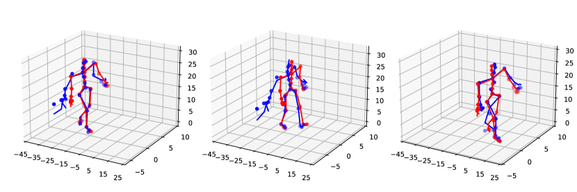
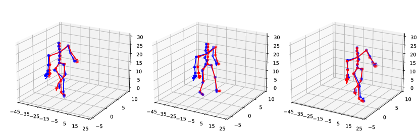
Figure 11: Example snapshots of Motion Capture with 50 time steps. Top: Prediction of GMN. Bottom: Prediction of PINGO. Ground truth in red, and prediction in blue.

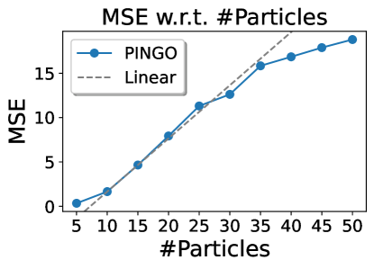
Figure 12: Mean squared error ($\times 10^{-2}$) w.r.t. number of particles.

Table 5: Mean squared error ($\times 10^{-2}$) of different numbers of particles w.r.t. layer number. (Reviewer xho3: Q1)

#Particle	Layer=6	Layer=7	Layer=8	Layer=9	Layer=10
30	13.38$\pm$0.07	13.21$\pm$0.03	13.27$\pm$0.20	13.50$\pm$0.21	13.51$\pm$0.15
40	17.25$\pm$0.12	16.44$\pm$0.09	16.72$\pm$0.32	16.65$\pm$0.24	16.90$\pm$0.08
50	18.82$\pm$0.07	18.85$\pm$0.16	18.80$\pm$0.11	18.65$\pm$0.15	18.82$\pm$0.10

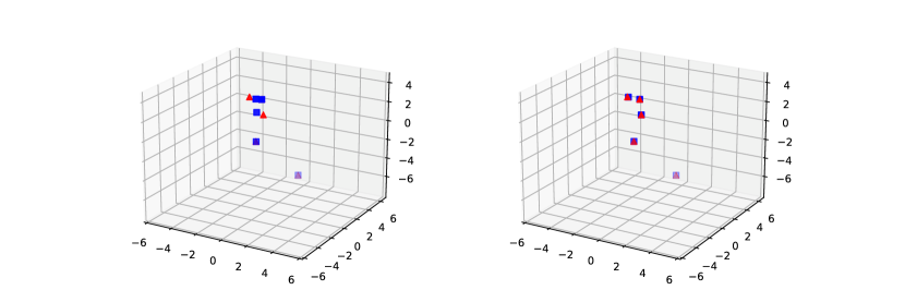
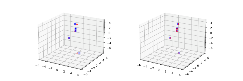
Figure 13: Example snapshots of N-body systems with 1000 time steps. Left: Prediction of EGNN. Right: Prediction of PINGO. Ground truth in red, and prediction in blue.

References

- Battaglia et al. [2016] P. W. Battaglia, R. Pascanu, M. Lai, D. Rezende, and K. Kavukcuoglu. Interaction networks for learning about objects, relations and physics. arXiv preprint arXiv:1612.00222, 2016.
- Bishnoi et al. [2022] S. Bishnoi, R. Bhattoo, S. Ranu, and N. Krishnan. Enhancing the inductive biases of graph neural ode for modeling dynamical systems. arXiv preprint arXiv:2209.10740, 2022.
- Brandstetter et al. [2021] J. Brandstetter, R. Hesselink, E. van der Pol, E. J. Bekkers, and M. Welling. Geometric and physical quantities improve e (3) equivariant message passing. arXiv preprint arXiv:2110.02905, 2021.
- Chen et al. [2018] T. Q. Chen, Y. Rubanova, J. Bettencourt, and D. Duvenaud. Neural ordinary differential equations. In S. Bengio, H. M. Wallach, H. Larochelle, K. Grauman, N. Cesa-Bianchi, and R. Garnett, editors, NeurIPS, pages 6572–6583, 2018.
- CMU [2003] CMU. Carnegie-mellon motion capture database. 2003. URL http://mocap.cs.cmu.edu.
- Coddington et al. [1956] E. A. Coddington, N. Levinson, and T. Teichmann. Theory of ordinary differential equations, 1956.
- Finzi et al. [2020a] M. Finzi, S. Stanton, P. Izmailov, and A. G. Wilson. Generalizing convolutional neural networks for equivariance to lie groups on arbitrary continuous data. In ICML, pages 3165–3176. PMLR, 2020a.
- Finzi et al. [2020b] M. Finzi, K. A. Wang, and A. G. Wilson. Simplifying hamiltonian and lagrangian neural networks via explicit constraints. In H. Larochelle, M. Ranzato, R. Hadsell, M. Balcan, and H. Lin, editors, NeurIPS, pages 13880–13889, 2020b.
- Fuchs et al. [2020] F. B. Fuchs, D. E. Worrall, V. Fischer, and M. Welling. Se (3)-transformers: 3d roto-translation equivariant attention networks. arXiv preprint arXiv:2006.10503, 2020.
- Gilmer et al. [2017] J. Gilmer, S. S. Schoenholz, P. F. Riley, O. Vinyals, and G. E. Dahl. Neural message passing for quantum chemistry. In ICML, pages 1263–1272, 2017.
- Gligorijević et al. [2021] V. Gligorijević, P. D. Renfrew, T. Kosciolek, J. K. Leman, D. Berenberg, T. Vatanen, C. Chandler, B. C. Taylor, I. M. Fisk, H. Vlamakis, et al. Structure-based protein function prediction using graph convolutional networks. Nature communications, 12(1):3168, 2021.
- Greydanus et al. [2019] S. Greydanus, M. Dzamba, and J. Yosinski. Hamiltonian neural networks. In H. M. Wallach, H. Larochelle, A. Beygelzimer, F. d’Alché-Buc, E. B. Fox, and R. Garnett, editors, NeurIPS, pages 15353–15363, 2019.
- Gruver et al. [2022] N. Gruver, M. A. Finzi, S. D. Stanton, and A. G. Wilson. Deconstructing the inductive biases of hamiltonian neural networks. In ICLR, 2022.
- Han et al. [2022] J. Han, Y. Rong, T. Xu, F. Sun, and W. Huang. Equivariant graph hierarchy-based neural networks. arXiv preprint arXiv:2202.10643, 2022.
- Huang et al. [2022] W. Huang, J. Han, Y. Rong, T. Xu, F. Sun, and J. Huang. Equivariant graph mechanics networks with constraints. arXiv preprint arXiv:2203.06442, 2022.
- Huang et al. [2020] Z. Huang, Y. Sun, and W. Wang. Learning continuous system dynamics from irregularly-sampled partial observations. In NeurIPS, 2020.
- Huang et al. [2021] Z. Huang, Y. Sun, and W. Wang. Coupled graph ODE for learning interacting system dynamics. In KDD, pages 705–715, 2021.
- Hutchinson et al. [2021] M. J. Hutchinson, C. Le Lan, S. Zaidi, E. Dupont, Y. W. Teh, and H. Kim. Lietransformer: equivariant self-attention for lie groups. In ICML, pages 4533–4543. PMLR, 2021.
- Karplus and McCammon [2002] M. Karplus and J. A. McCammon. Molecular dynamics simulations of biomolecules. Nature structural biology, 9(9):646–652, 2002.
- Kingma and Ba [2015] D. P. Kingma and J. Ba. Adam: A method for stochastic optimization. In ICLR, 2015.
- Kipf et al. [2018] T. Kipf, E. Fetaya, K.-C. Wang, M. Welling, and R. Zemel. Neural relational inference for interacting systems. arXiv preprint arXiv:1802.04687, 2018.
- Köhler et al. [2019] J. Köhler, L. Klein, and F. Noé. Equivariant flows: sampling configurations for multi-body systems with symmetric energies. arXiv preprint arXiv:1910.00753, 2019.
- Lutter et al. [2019] M. Lutter, C. Ritter, and J. Peters. Deep lagrangian networks: Using physics as model prior for deep learning. In ICLR, 2019.
- Mrowca et al. [2018] D. Mrowca, C. Zhuang, E. Wang, N. Haber, L. Fei-Fei, J. B. Tenenbaum, and D. L. Yamins. Flexible neural representation for physics prediction. arXiv preprint arXiv:1806.08047, 2018.
- Poli et al. [2019] M. Poli, S. Massaroli, J. Park, A. Yamashita, H. Asama, and J. Park. Graph neural ordinary differential equations. arXiv preprint arXiv:1911.07532, 2019.
- Sanchez-Gonzalez et al. [2019] A. Sanchez-Gonzalez, V. Bapst, K. Cranmer, and P. W. Battaglia. Hamiltonian graph networks with ODE integrators. arXiv preprint arXiv:1909.12790, 2019.
- Sanchez-Gonzalez et al. [2020] A. Sanchez-Gonzalez, J. Godwin, T. Pfaff, R. Ying, J. Leskovec, and P. Battaglia. Learning to simulate complex physics with graph networks. In ICML, pages 8459–8468. PMLR, 2020.
- Satorras et al. [2021] V. G. Satorras, E. Hoogeboom, and M. Welling. E (n) equivariant graph neural networks. In ICML, pages 9323–9332. PMLR, 2021.
- Schütt et al. [2021] K. Schütt, O. Unke, and M. Gastegger. Equivariant message passing for the prediction of tensorial properties and molecular spectra. In ICML, pages 9377–9388. PMLR, 2021.
- Siciliano et al. [2009] B. Siciliano, L. Sciavicco, L. Villani, and G. Oriolo. Robotics. Springer London, 2009. doi: 10.1007/978-1-84628-642-1. URL https://doi.org/10.1007/978-1-84628-642-1.
- Thomas et al. [2018] N. Thomas, T. Smidt, S. Kearnes, L. Yang, L. Li, K. Kohlhoff, and P. Riley. Tensor field networks: Rotation-and translation-equivariant neural networks for 3d point clouds. arXiv preprint arXiv:1802.08219, 2018.
- Torng and Altman [2019] W. Torng and R. B. Altman. Graph convolutional neural networks for predicting drug-target interactions. Journal of chemical information and modeling, 59(10):4131–4149, 2019.
- Wen et al. [2022] S. Wen, H. Wang, and D. N. Metaxas. Social ODE: multi-agent trajectory forecasting with neural ordinary differential equations. In ECCV, volume 13682, pages 217–233, 2022.
- White and Frenk [1985] S. White and C. Frenk. Numerical techniques for large cosmological n-body simulations. The Astrophysical Journal Supplement Series, 57:241–260, 1985.
- Yildiz et al. [2022] Ç. Yildiz, M. Kandemir, and B. Rakitsch. Learning interacting dynamical systems with latent gaussian process odes. In NeurIPS, 2022.
- Yuan et al. [2021] Y. Yuan, X. Weng, Y. Ou, and K. Kitani. Agentformer: Agent-aware transformers for socio-temporal multi-agent forecasting. In ICCV, pages 9793–9803, 2021.
- Zhu et al. [2022] A. Zhu, P. Jin, B. Zhu, and Y. Tang. On numerical integration in neural ordinary differential equations. In ICML, pages 27527–27547, 2022.