Robust features of QCD phase diagram through a Contact Interaction model for quarks: A view from the effective potential

Abstract

Our research delves into the QCD phase diagram in the temperature $T$ and quark chemical potential $\mu$ plane. We use a unique confining contact interaction effective model of quark dynamics that maintains the QCD symmetry intact. By embedding the model into a Schwinger-Dyson equations framework, within a Landau gauge rainbow-ladder-like truncation, we derive the gap equation. In order to accurately regulate the said equation, we utilize the Schwinger optimal time regularization scheme. We further derive the effective potential of the model by integrating the gap equation over the dynamical mass, which along with the confining length scale serve as parameters for the chiral and confinement deconfinement phase transitions, respectively. A cross-over transition is observed at low $\mu$ and above a critical value of the temperature $T_{c}$, whilst a first order phase transition is found for low $T$ at high density. The critical end point is estimated to be located at $(\mu_{E}/T_{c,0}=1.6,T_{E}/T_{c,0}=0.42)$, which falls within the range of other QCD effective models predictions. $T_{c,0}=208$ MeV is the critical temperature at vanishing $\mu$. Screening effects of the medium which dilute the strength of the effective coupling are considered by including the vacuum polarization contribution due to quarks at high temperatures into the framework. It locates the critical end point at $(\mu^{E}_{c}/T_{c}\approx 2.6,T^{E}_{c}/T_{c}\approx 0.57)$, which hints for a deeper analysis of screening effects on models of this kind.

Keywords: Chiral symmetry breaking, Confinement-Deconfinement transition, Schwinger-Dyson equation, Finite temperature and density, QCD phase diagram

1 Introduction

Quantum Chromodynamics (QCD) is the theory that describes the color interactions among quarks and gluons. It plays a crucial role in understanding the symmetric and peculiar nature of the universe. Asymptotic freedom [1, 2] and quark confinement [3] are the two fundamental features of QCD. In the high-energy domain, or asymptotic freedom realm, quarks interact weakly at short distances inside hadrons. However, at larger distances, or in the low-energy domain, quarks are strongly interacting and cannot exist in isolation (i.e., the quark are confined inside hadrons). In addition to quark confinement, low-energy QCD also exhibits another important phenomenon, which is the dynamical breaking of chiral symmetry, and its consequence, the dynamical mass generation of constituent quarks. Studying low-energy QCD at finite temperature $T$ and density parametrized by a quark or baryon chemical potential $\mu$ has significant implications for understanding the phase transition that took place in the early universe a few microseconds after the Big Bang. The transition from hadronic matter to quark-gluon plasma [4], quarkyonic matter [5, 6], neutron star formation [7], and the color-flavor locked (CFL) region [8, 9, 10] are the subjects of current interest. The advancements in technology and experimental facilities have enabled us to study the properties of QCD at high temperatures and relatively low densities. The recent upgrades in detectors at various research facilities such as the sPHENIX detector and complementary STAR upgrades at RHIC, as well as upgraded detectors at ALICE, ATLAS, CMS, and LHCb, have paved the way for a multimessenger era for hot QCD (see for detail in recent review [11]), which is based on the combined constraining power of low-energy hadrons, jets, thermal electromagnetic radiation, heavy quarks, and exotic bound states. The increased luminosity at the LHC and other experimental facilities such as RHIC and the Compact Baryonic Matter (CBM) experiments, along with the facilities under construction in Fair [12] and NICA [13] will also provide a unique opportunity to study the phase transition from hadronic matter to quark-gluon plasma and the related phenomena.

At temperatures close to zero, the color-singlet hadrons are widely believed to be the fundamental degrees of freedom of low-energy QCD. However, once the temperature exceeds a critical value $T_{c}$, the interaction weakens, leading hadrons to melt into a new phase. In this phase, quarks and gluons become the new degrees of freedom, and the chiral symmetry is restored and quarks become deconfined. Several methods, including Lattice QCD calculations [14, 15, 16, 17, 18, 19, 20], Schwinger-Dyson equations [21, 22, 23, 24, 25, 26, 27, 28, 29, 30, 31], and other effective models of low-energy QCD [32, 33, 34, 35, 25, 36, 37, 38], have all suggested that the transition at hand is a cross-over when a finite current quark mass $m$ is taken into account; otherwise, chiral limit calculations show a second-order phase transition. In any case, as the quark chemical potential $\mu$ is raised, the same physical behavior persists , but the nature of the phase transition changes from a cross-over to a first-order transition at the critical end point (CEP) in the QCD phase diagram, which is typically illustrated on the $T-\mu$ plane. The exact location of the critical endpoint is not predicted so far and has become a hot scientific topic which has deserved the design of experiments to observe it. However, if we represent the position of this point as  $(\mu_{E}/T_{c},T_{E}/T_{c})$, where $T_{c}$ denotes the temperature at which chiral symmetry restoration occurs for $\mu=0$, then it is reasonable to claim that model calculations [40, 41, 42, 43, 44, 45, 46, 23, 25, 38] locate this point in the region  $(\mu_{E}/T_{c}=1.0-2.0,T_{E}/T_{c}=0.4-0.8)$ considering $N_{f}=2$ flavors. However, mathematical extensions of lattice techniques [47, 48, 49, 50] predict that the point is located around approximately between $(\mu_{E}/T_{c}=1.0-1.4,T_{E}/T_{c}=0.9)$ for simulations including the strange quark. Background electromagnetic fields also affect the QCD phase diagram, since the critical temperature $T_{c}$ decreases with the increase of electric and magnetic fields [31, 27, 30, 51, 52, 53, 54]. Furthermore, the QCD phase transitions under consideration are also sensitive to the number of light quark flavors, as highlighted, for instance, in Ref. [31], where an increase in the number of light quark flavors leads to a suppression of the critical line between chiral symmetry broken and restoration phases in the phase diagram.

Our main goal in this work is to study the chiral symmetry breaking-restoration and confinement-deconfinement phase transitions, and chart out the QCD phase diagram. To achieve this, we use a confining regularization version of the Nambu-Jonal-Lasinio (NJL) model which consists in a symmetry-preserving vector-vector contact interaction model of quarks, in the Schwinger-Dyson equations framework in the Landau gauge with a Schwinger optimal time regularization scheme, at finite temperature $T$ and chemical potential $\mu$. As it is well-known, the NJL model [32, 55, 33] is quite successful in providing the properties of low-energy mesons. The most significant aspect of this model is that it exhibits spontaneous chiral symmetry. Unfortunately, the NJL model does not support quark confinement and suffers from an unphysical quark-antiquark threshold. To construct the confining version of the NJL model, the first attempt was made by [56] to regularize it by introducing an infrared cut-off $\tau_{ir}=1/\Lambda{ir}$ along with an ultraviolet cut-off $\tau_{uv}=1/\Lambda_{uv}$. The infrared cut-off removes the unphysical quark-antiquark production threshold, and by introducing a finite value for the infrared cut-off, confinement is implemented. Later on, a similar idea was promoted by [57, 58, 59], by removing the poles from the quark propagator, which implies that the excitation represented by a pole-less propagator is confined. With the particular choice of values for $\tau_{ir}=(0.24{\rm GeV})^{-1}$ and $\tau_{uv}=(0.905{\rm GeV})^{-1}$, along with other model parameters, they studied the properties of $\pi$ and $\rho$ mesons, and their diquark partners, with approximately up to a $10$ percent error with the experimentally measured values. Here, we are promoting the regularization procedure outlined in references [59, 60] to explore the QCD phase diagram at finite temperature and density. Under similar assumptions, the confining scale $\tau_{ir}(T)$ has been used as an order parameter for the confinement-deconfinement transition at finite temperature $T$ [61], as well as in the presence of background electromagnetic fields $\tau_{ir}(T,eB,eE)$ [62, 30, 31]. In our considerations, the gap equation obtained from this model can be integrated with respect to the dynamically generated mass, hence defining the effective thermodynamic potential of the present contact interaction model [63]. Here, we are interested in analyzing the traits of the chiral symmetry breaking and restoration and confinement-deconfinement transitions at finite temperature and density from this effective potential. In the present work, we consider the confining length as temperature and chemical potential dependent, and denote it as $\tau_{ir}(T,\mu)$. It is important to note that in this model, chiral symmetry restoration and deconfinement occur simultaneously [64, 62, 30, 31].

The remaining of this manuscript is organized as follows: In Section 2, we present the general formalism for the contact interaction model, the QCD gap equation, and the effective potential. In Section 3, we discuss the gap equation and effective potential at finite $T$ and $\mu$. Section 4 presents the numerical solutions for the gap equation and the effective potential, and we sketch the phase diagram in the $T-\mu$ plane. In Section 5 we explore the screening effects of the medium by including vacuum polarization effects in the coupling due to the quarks in the high-$T$ domain. In the last section, Section 6, we provide a summary and future perspectives of our work.

2 General Formalism

2.1 Gap equation and Effective Potential in vacuum

We start from the Schwinger-Dyson Equation for the dressed quark propagator:

$$S^{-1}(p) =S^{-1}_{0}(p)+\Sigma(p)\,,$$ (1)

where

$$S_{0}(p)=(\not{p}-m+i\epsilon)^{-1}$$

represents the bare quark propagator in Minkowski space, $S(p)$ denotes the dressed quark propagator, while the self-energy $\Sigma(p)$ can be expressed as follows:

$$\Sigma(p)=-i\int\frac{d^{4}k}{(2\pi)^{4}}g^{2}\Delta_{\mu\nu}(q)\frac{\lambda^{a}}{2}\gamma_{\mu}S(k)\frac{\lambda^{a}}{2}\Gamma_{\nu}(p,k)\,.$$ (2)

Here, the dressed quark-gluon vertex is denoted by $\Gamma_{\nu}(k,p)$, and the QCD coupling constant is represented by $g^{2}$. The gluon propagator in the Landau gauge can be expressed as

$$\Delta_{\mu\nu}(q)=-i\frac{\Delta(q)}{q^{2}}\left(g_{\mu\nu}-\frac{q_{\mu}q_{\nu}}{q^{2}}\right),$$

where $g_{\mu\nu}$ is the metric tensor in Minkowski space, $\Delta(q)$ is the gluon dressing function, and $q=k-p$ is the gluon four-momentum. The current quark mass is represented by $m$, which can be set to zero (i.e., $m=0$) in the chiral limit. Additionally, $\lambda^{a}$’s refer to the Gell-Mann matrices, which satisfy the following identity in the ${\rm SU(N_{c})}$ representation:

$$\sum^{8}_{a=1}\frac{{\lambda}^{a}}{2}\frac{{\lambda}^{a}}{2}=\frac{1}{2}\left(N_{c}-\frac{1}{N_{c}}\right)I,$$

where $I$ is the unit matrix. In this study, we employ a flavor-dependent confining contact interaction model for the gluon propagator in the infrared region, where the gluons spontaneously acquire a mass $m_{g}$ [65, 66, 67, 57, 68]. It has been previously described in detail in [31, 38] and it is explicitly given by:

$$g^{2}\frac{\Delta(q)}{q^{2}}\Bigg{|}_{q\rightarrow 0} = \frac{4\pi\alpha_{\rm ir}}{m_{G}^{2}}\sqrt{1-\frac{(N_{f}-2)}{\mathcal{N}_{f}^{c}}}=\alpha_{\rm eff}\sqrt{1-\frac{(N_{f}-2)}{\mathcal{N}_{f}^{c}}}=\alpha_{\rm eff}(N_{f})\,.$$ (3)

In this particular scenario, the strength parameter for the infrared-enhanced interaction is represented by $\alpha_{\rm ir}=0.93\pi$, while the gluon mass scale $mg=800$ MeV is chosen from [69]. Furthermore, $\mathcal{N}_{f}^{c}$ denotes the guessed critical number of flavors, as discussed in previous works [31, 38]. For this model, the dynamical quark mass function remains constant, while the dressed quark propagator can be written in the following form [70, 38] :

$$S(k)=\frac{\not{k}+M}{k^{2}-M^{2}+i\epsilon}.$$ (4)

Here, $M$ is the dynamical quark mass. Substituting Eqs. (2) -(4) into Eq.(1) and taking the trace over the Dirac, color, and flavor components, we have

$$M=m+4i\alpha^{N_{c}}_{\rm eff}(N_{f})\int{\frac{d^{4}k}{(2\pi)^{4}}\frac{M}{k^{2}-M^{2}+i\epsilon}},$$ (5)

where

$$\alpha^{N_{c}}_{\rm eff}(N_{f})=\frac{\alpha_{\rm eff}(N_{f})}{2}\left(N_{c}-\frac{1}{N_{c}}\right),$$ (6)

is the color-flavor effective coupling. For $N_{c}=3$ and $N_{f}=2$, Eq. (6) reduces to $\alpha^{N_{c}}_{\rm eff}(N_{f})\rightarrow 4\alpha_{\rm eff}/3$, and the gap equation Eq. (5) can be written as:

$$M=m+\frac{16\alpha_{\rm eff}i}{3}\int{\frac{d^{4}k}{(2\pi)^{4}}\frac{M}{k^{2}-M^{2}+i\epsilon}}.$$ (7)

It should be noted that the effective coupling $\alpha_{\rm eff}$ in Eq. (7) must exceed its critical value $\alpha^{c}_{eff}$, to describe dynamical chiral symmetry breaking. When $\alpha_{\rm eff}$ is greater than its critical value $\alpha^{c}_{\rm eff}$, a nontrivial solution to the QCD gap equation bifurcates from the trivial one, see for instance Ref. [71].

The four-dimensional momentum integral in Eq. (7), can be tackled by splitting the four-momentum into time and space components. We denote the space part by a bold face latter k and the time part by $k_{0}$. Thus, Eq. (7) can be written as

$$M=m+\frac{16\alpha_{eff}Mi}{3}\int_{0}^{\infty}\frac{d^{3}\textbf{k}}{(2\pi)^{4}}\int_{-\infty}^{+\infty}{\frac{dk_{0}}{{k_{0}}^{2}-E_{k}^{2}+i\epsilon}}.$$ (8)

Here, $E_{k}=\sqrt{{|\textbf{k}}|^{2}+M^{2}}$ in which $E_{k}$ denotes the energy per particle and k is the $3$-momentum. On integrating over the time component of Eq. (8), we get the following expression:

$$M=m+\frac{16\alpha_{\rm eff}Mi}{3}\int_{0}^{\infty}\frac{d^{3}\textbf{k}}{(2\pi)^{4}}\frac{\pi}{iE_{k}}$$ (9)

In spherical polar coordinates $d^{3}\textbf{k}=\textbf{k}^{2}d\textbf{k}\sin\theta d\theta d\phi$ and performing the angular integration, we have from Eq. (9):

$$M=m+\frac{4\alpha_{\rm eff}M}{3\pi^{2}}\int_{0}^{\infty}d\textbf{k}\frac{\textbf{k}^{2}}{\sqrt{{\textbf{k}}^{2}+M^{2}}}.$$ (10)

The integral presented in Eq. (10) is divergent and necessitates regularization. One way to accomplish this is by using the Schwinger proper time regularization scheme, which involves introducing an infrared cut-off of $\tau_{ir}=1/\Lambda_{ir}$ in conjunction with an ultraviolet cut-off $\tau_{uv}=1/\Lambda_{uv}$ [56, 57, 60], which allows us to use the identity

$$\frac{1}{A^{n}}=\frac{1}{\Gamma(n)}\int^{\infty}_{0}d\tau\tau^{n-1}e^{-\tau A},$$ (11)

with $\Gamma(n)$ is the Gamma function. In our present case, we substitute $A=\textbf{k}^{2}+M^{2}$ and $n=\frac{1}{2}$. Thus, we obtain the following expression:

$$\frac{1}{\sqrt{\textbf{k}^{2}+M^{2}}} = \int^{\infty}_{0}d\tau\frac{e^{-\tau(\textbf{k}^{2}+M^{2})}}{\sqrt{\pi\tau}}\rightarrow\int_{\tau^{2}_{uv}}^{\tau^{2}_{ir}}\frac{d\tau}{\sqrt{\pi\tau}}e^{-\tau(\textbf{k}^{2}+M^{2})}$$ (12)

$$= \frac{{\rm Erf}(\sqrt{k^{2}+M^{2}}\,\tau_{ir})-{\rm Erf}(\sqrt{k^{2}+M^{2}}\,\tau_{uv})}{\sqrt{k^{2}+M^{2}}}.$$

The pole in this expression is situated at $\textbf{k}^{2}=-M^{2}$, but we observe that precisely ath the pole both the numerator and denominator vanish, thereby causing the pole to disappear from the quark propagator. The ultraviolet regulator, $\tau_{uv}=\Lambda^{-1}_{uv}$, plays a dynamical role in setting the scale for all dimensional quantities. The infrared regulator, denoted as $\tau_{ir}=\Lambda^{-1}_{ir}$, has a non-zero value that facilitates the interpretation of confinement [56, 60, 59]. As such, $\tau_{ir}$ is often referred to as the confinement scale [61, 62, 30, 31]. Upon analyzing Eq. (12), it becomes evident that the propagator does not possess any real or complex poles, thereby aligning with the definition of confinement. In other words, an excitation described by a pole-less propagator would never attain its mass-shell [56]. Upon inserting Eq. (12) in Eq. (10) and performing $k$-integration, the gap equation Eq. (10) is reduced to:

$$M=m+\frac{\alpha_{eff}M}{3\pi^{2}}\bigg{(}\frac{e^{-M^{2}\tau_{ir}^{2}}}{\tau_{ir}^{2}}+\frac{e^{-M^{2}\tau_{uv}^{2}}}{\tau_{uv}^{2}}-M^{2}{\rm Ei}(-M^{2}\tau_{ir}^{2})+M^{2}{\rm Ei}(-M^{2}\tau_{uv}^{2})\bigg{)},$$ (13)

where

$${\rm Ei}(x)=\int^{x}_{-\infty}\frac{e^{t}}{t}dt,$$

is the exponential integral function. The quark-antiquark condensate in this model is defined as:

$$-\langle\bar{q}q\rangle=\frac{M-m}{\alpha_{\rm eff}}.$$ (14)

Re-arranging the gap equation Eq. (13) and integrating over $M$, we have

$$\Omega(M)=\int dM\bigg{[}\frac{M-m}{\alpha_{\rm eff}}-\frac{M}{3\pi^{2}}\left(\frac{e^{-M^{2}\tau_{ir}^{2}}}{\tau_{ir}^{2}}+\frac{e^{-M^{2}\tau_{uv}^{2}}}{\tau_{uv}^{2}}-M^{2}{\rm Ei}(-M^{2}\tau_{ir}^{2})+M^{2}{\rm Ei}(-M^{2}\tau_{uv}^{2})\right)\bigg{]}$$

$$=\frac{(M-m)^{2}}{2\alpha_{\rm eff}}-\frac{1}{12\pi^{2}}\bigg{(}\frac{e^{-M^{2}\tau_{ir}^{2}}(1-M^{2}\tau_{ir}^{2})}{\tau_{ir}^{4}}+\frac{e^{-M^{2}\tau_{uv}^{2}}(-1+M^{2}\tau_{uv}^{2})}{\tau_{uv}^{4}}$$

$$-M^{4}{\rm Ei}(-M^{2}\tau_{ir}^{2})+M^{4}{\rm Ei}(-M^{2}\tau_{uv}^{2})\bigg{)}+constant,$$ (15)

where $\Omega(M)$ is the effective potential in vacuum.

In the next subsection, we discuss the gap equation and the contact interaction effective potential at finite temperature $T$ and chemical potential $\mu$.

2.2 Gap equation and Effective Potential at finite $T$ and $\mu$

The gap equation (Eq. (7)) at finite temperature $T$ and quark chemical potential $\mu$ can be obtained in the imaginary-time formalism by adopting the following standard convention for momentum integration:

$$\int\frac{d^{4}k}{i(2\pi)^{4}}f(k_{0},{\bf{k}})\rightarrow T\sum_{n}\int\frac{d^{3}k}{(2\pi)^{3}}f(i\omega_{n}+\mu,\bf{k}),$$ (16)

where $\omega_{n}=(2n+1)\pi T$ are the fermionic Matsubara frequencies. Using Eq. (16) in Eq. (7) and after some straightforward algebra, the gap equation at finite $T$ and $\mu$ is given by:

$$M = m+\frac{4\alpha_{\rm eff}M}{3\pi^{2}}\int^{\infty}_{0}\frac{d^{3}\textbf{k}}{(2\pi)^{3}}\frac{1}{\sqrt{\textbf{k}^{2}+M^{2}}}(1-n_{F}(T,\mu)+\bar{n}_{F}(T,\mu))).$$ (17)

The first term of Eq. (17) is similar to Eq. (7), the vacuum term, but modified by the thermo-chemical effects of the medium. The functions $n_{F}(T,\mu)$ and $\bar{n}_{F}(T,\mu)$ represent the Fermi occupation numbers for the quarks and antiquarks, respectively, and are defined as follows:

$$n_{F}(T,\mu)=\frac{1}{e^{(\sqrt{\textbf{k}^{2}+M^{2}}-\mu)/T}+1},\hskip 11.38109pt\bar{n}_{F}(T,\mu)=\frac{1}{e^{(\sqrt{\textbf{k}^{2}+M^{2}}+\mu)/T}+1}.$$ (18)

By separating the vacuum component from the medium and utilizing proper time regularization as in Eq. (12), the gap equation in Eq. (18) can be simplified as follows:

$$M = m+\frac{\alpha_{\rm eff}M}{3\pi^{2}}\bigg{(}\frac{e^{-M^{2}\tau_{ir}^{2}}}{\tau_{ir}^{2}}+\frac{e^{-M^{2}\tau_{uv}^{2}}}{\tau_{uv}^{2}}-M^{2}{\rm Ei}(-M^{2}\tau_{ir}^{2})+M^{2}{\rm Ei}(-M^{2}\tau_{uv}^{2})\bigg{)}$$ (19)

$$- \frac{4\alpha_{\rm eff}M}{3\pi^{2}}\int_{0}^{\infty}d\textbf{k}\frac{\textbf{k}^{2}}{\sqrt{\textbf{k}^{2}+M^{2}}}\left[n_{F}(T,\mu)+\bar{n}_{F}(T,\mu)\right].$$

By setting $\mu=T=0$ in Eq. (19), we obtain $n{F}=\bar{n}{F}=0$, thus recovering the gap equation in a vacuum Eq. (13). The thermo-chemical contact interaction effective potential can be determined by integrating Eq. (19) over $M$, resulting in the following expression:

$$\Omega(M,T,\mu) = \frac{(M-m)^{2}}{2\alpha_{eff}}-\frac{1}{12\pi^{2}}\bigg{(}\frac{e^{-M^{2}\tau_{ir}^{2}}(1-M^{2}\tau_{ir}^{2})}{\tau_{ir}^{4}}+\frac{e^{-M^{2}\tau_{uv}^{2}}(-1+M^{2}\tau_{uv}^{2})}{\tau_{uv}^{4}}$$ (20)

$$- M^{4}{\rm Ei}(-M^{2}\tau_{ir}^{2})+M^{4}{\rm Ei}(-M^{2}\tau_{uv}^{2})\bigg{)}$$

$$- \frac{4}{3\pi^{2}}\int_{0}^{\infty}d\textbf{k}\textbf{k}^{2}\bigg{(}T\log\left[1+\exp(-\frac{\sqrt{\textbf{k}^{2}+M^{2}}-\mu}{T})\right]$$

$$+ T\log\left[1+\exp(-\frac{\sqrt{\textbf{k}^{2}+M^{2}}+\mu}{T})\right]\bigg{)}.$$

It is important to recall that the physical state with the highest stability corresponds to the global minimum of the effective thermodynamic potential. This means that the state with the smallest value of $\Omega$, determined by satisfying the conditions $\partial\Omega/\partial M=0$ and $\partial^{2}\Omega/\partial M^{2}\geq 0$, is considered the most stable. Let us discuss the scenario where the temperature is zero. As we approach the limit of $T\rightarrow 0$, the thermal factor attributed to quarks in Eq. (20) is converted into the step function $\Theta(\mu-E_{k})$, while the thermal factor associated with antiquark becomes zero, as $E_{k}+\mu>0$ is always true. Thus, the effective potential in the limit of $T\rightarrow 0$ and at finite chemical potential $\mu$ is given by:

$$\Omega(M,\mu) = \frac{(M-m)^{2}}{2\alpha_{eff}}-\frac{1}{12\pi^{2}}\bigg{(}\frac{e^{-M^{2}\tau_{ir}^{2}}(1-M^{2}\tau_{ir}^{2})}{\tau_{ir}^{4}}+\frac{e^{-M^{2}\tau_{uv}^{2}}(-1+M^{2}\tau_{uv}^{2})}{\tau_{uv}^{4}}$$ (21)

$$- M^{4}{\rm Ei}(-M^{2}\tau_{ir}^{2})+M^{4}{\rm Ei}(-M^{2}\tau_{uv}^{2})\bigg{)}$$

$$- \frac{4}{3\pi^{2}}\int_{0}^{k_{F}}d\textbf{k}\textbf{k}^{2}\left(\mu-\sqrt{\textbf{k}^{2}+M^{2}}\right)\Theta(\mu-\sqrt{\textbf{k}^{2}+M^{2}}),$$

where $k_{F}=\sqrt{(\mu^{2}-M^{2})}\Theta(\mu-M)$ is the Fermi momentum. We assume that the chemical potential $\mu$ is greater than or equal to the mass $M$ of the particles in the system. Notice that Eq. (21) relies on two contributions - the energy of the positive condensate field (represented by the first term), and the negative contribution stemming from the Dirac sea (represented by the second term). The first term tends to favor the proximity of $M$ to $m$, whereas the second term favors higher values of $M^{2}$. Next, we take the derivative of the thermodynamic potential Eq. (21) with respect to the effective mass $M$ and equate it to zero. This results in the gap equation at zero-temperature and finite chemical potential:

$$\frac{M-m}{\alpha_{\rm eff}}=\frac{M}{12\pi^{2}}\bigg{(}\frac{e^{-M^{2}\tau_{ir}^{2}}}{\tau_{ir}^{2}}+\frac{e^{-M^{2}\tau_{uv}^{2}}}{\tau_{uv}^{2}}-M^{2}{\rm Ei}(-M^{2}\tau_{ir}^{2})+M^{2}{\rm Ei}(-M^{2}\tau_{uv}^{2})\bigg{)}~{}{\rm for}~{}\mu<M,$$

$$\frac{M-m}{\alpha_{\rm eff}}=\frac{4M}{3\pi^{2}}\int_{k_{f}}^{\infty}d\textbf{k}\frac{\textbf{k}^{2}}{\sqrt{\textbf{k}^{2}+M^{2}}}~{}{\rm for}~{}\mu>M.$$ (22)

In the upcoming section, we showcase the numerical solution to the gap equation and effective potential in both vacuum and at finite temperature and chemical potential. Additionally, we depict the QCD phase diagram for the chiral symmetry breaking-restoration and confinement-deconfinement transition in the $T-\mu$ plane.

3 Numerical Results

In this Section, we discuss the numerical solution of the gap equation and the effective potential at finite temperature and chemical potential. We also sketch the phase diagram in $T-\mu$ plane. We use the following set of parameters: $\tau_{ir}=(240{\rm MeV})^{-1}$, $\tau_{uv}=(905{\rm MeV})^{-1}$, $\alpha_{\rm eff}=5.739\times 10^{-5}{\rm MeV}^{-2}$, and a bare quark mass $m_{u/d}=7{\rm MeV}$. The values of these parameters are taken from [57], which were determined by fitting them to the appropriate values for the $\pi$ ans $\rho$ mesons properties. The solution of the gap Eq. (13) in the chiral limit gives a dynamical quark mass $M=0.358$ MeV and with current quark mass $m=7$ MeV, it is $M=0.368$. The vacuum effective potential, Eq. (15), as a function of $M$ is shown in Fig. 1, in the chiral limit ($m=0$) and with bare quark mass ($m=7$ MeV). In this case one obtains that the minima of $\Omega_{vac}$ are precisely located at the solutions to the gap equation, while the trivial solution $M=0$ is a maximum in both cases. The minimum value for positive mass corresponds to the global minimum of effective potential, so it is the stable dynamical quark mass.

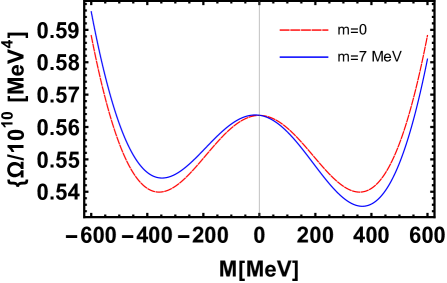
Figure 1: Behavior of the effective potential in the chiral limit and with bare mass $m=7$ MeV as a function of the dynamical mass $M$ at $T=\mu=0$. It clearly demonstrates the dynamical breaking of chiral symmetry. In the chiral limit, the global minimum occurs at $M=\pm 358$ MeV, while in case red in which we include the current quark mass, the minimum is at $M=\pm 367$ MeV.

Next, we solve the gap equation Eq. (19) and effective potential Eq. (20), at finite temperature $T$ but keeping $\mu=0$. The dynamical mass as a function of $T$ is plotted in Fig. 2(2(a)) which decreases with the increase in $T$. The thermodynamic potential as a function of $M$ for various values of the temperature $T$ is depicted in Fig. 2(2(b)) which shows that the global minima are shifted toward lower values of the dynamical mass $M$ upon increasing the temperature and, at some critical temperature $T=T_{c}=208$ MeV, the thermodynamic potential has minimum values at the lowest values of the effective mass $M$, which gives a clear signal about chiral symmetry restoration: the dynamical mass vanishes and the bare mass survives. The nature of the transition is smooth cross-over. It is also clear from Fig. 2(2(c)) that the thermal gradient of the effective mass $M$ peaks at $T_{c}=208$ MeV.

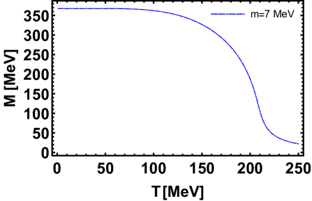
(a)

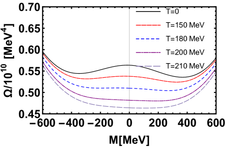
(b)

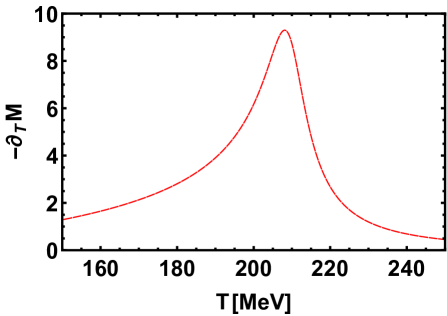
(c)

Figure 2: (2(a)) The dynamical quark mass $M$ as a function of temperature $T$. (2(b)) Effective potential as a function of $M$ for various $T$ at $\mu=0$. These plots demonstrate that at and above $T_{c}$, minima are shifted towards lower $M$, which clearly indicates the restoration of chiral symmetry. (2(c)) The thermal-gradient of effective mass $M$; the peak of the gradient is at $T_{c}\approx 208$ MeV, which is the critical temperature above which chiral symmetry is restored.

The thermodynamic potential at  $T=0$ for different values of the chemical potentials $\mu$ as a function of the effective quark mass $M$ is shown in Fig. 3(3(a)). This is a first order phase transition, where the thermodynamic potential has multiple minima and the global minimum switches from one minimum to another at and above $\mu_{c}$. In Fig. 3(3(b)), we plotted the effective mass $M$ i.e., the solution of Eq. (22) as a function of chemical potential $\mu$ which clearly indicates the chiral symmetry restoration discontinuously at and above $\mu_{c}\approx 380$ MeV.

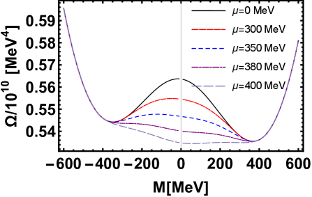
(a)

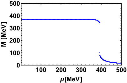
(b)

Figure 3: (3(a)) Behaviour of the effective potential as function of the dynamical mass for various values of the chemical potential. It shows the transition from chiral symmetry broken to the chiral restored phase through a first order phase transition, where the thermodynamic potential has multiple minima and the global minimum switches from one minimum to another. (3(b)) Behavior of the dynamical mass $M$ as a function of chemical potential $\mu$. The dynamical mass remains constant until $\mu_{c}\approx 380$ MeV, where it drops discontinuously and the chiral symmetry is restored via a first order phase transition.

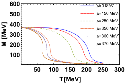
(a)

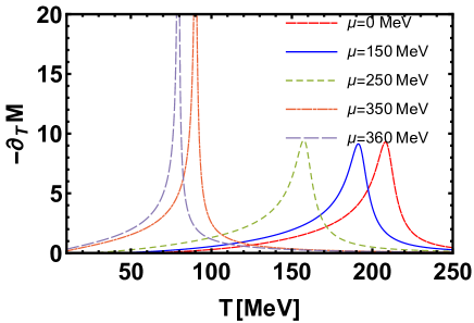
(b)

Figure 4: (2(a)) Dynamical quark mass $M$ as a function of temperature and for various values of the chemical potential. (2(b)) The thermal gradient of the dynamical mass as a function of temperature for various values of the chemical potential.

As for the dynamical $M$ as a function of temperature $T$ for various values of the chemical potential $\mu$, results are shown in Fig. 4 (4(a)). The dynamical mass $M$ decreases monotonically with the temperature and suppresses as we increase the chemical potential $\mu$. At and above a critical value of the chemical potential $\mu_{c}\approx 350$ MeV the mass plateau shows a discontinuity. The critical temperature $T_{c}(\mu)$ at various values of the chemical potential can be obtained from the thermal gradient of the dynamical mass, which is shown in Fig. 4 (4(b)). The Critical End Point (CEP), where the cross-over phase transition ends and the first order phase transition begins, is therefore obtained from the divergence of the mass gradient at particular chemical potential and temperature. In this case, it happens at $(\mu^{E}_{c}\approx 350{\rm MeV},T^{E}_{c}\approx 90{\rm MeV})$. The effective potential at the CEP is depicted in the Fig. 5.

The confinement scale and its thermal gradient as a function of temperature for various values of the chemical potential is shown in Fig. (6). The critical temperature $T_{c}$ for the confinement-deconfinement transition for various values of the chemical potential $\mu$ can be obtained from the peak of the thermal gradient. It is clear from the thermal gradients of both the dynamical mass $M$ and the confinement scale $\hat{\tau}^{-1}_{ir}$ that the chiral symmetry breaking-restoration and confinement-deconfinement transition occur simultaneously. We have constructed a phase diagram the $T-\mu$ plane, which reveals that at finite temperature $T$ but zero chemical potential $\mu$, chiral symmetry is broken for temperatures $T\leq T_{c}\approx 208$ MeV. However, above this threshold, the symmetry is restored and deconfinement occurs. The order of the phase transition is a cross-over. On the other hand, when we consider finite chemical potential $\mu$ and zero temperature $T$, we find that chiral symmetry is broken and confinement settles below a critical chemical potential $\mu_{c}\approx 380$ MeV, while above this value, it is restored and deconfinement occurs, but the transition is of first-order. Based on Fig. 7, we confirmed that the cross-over line in the phase diagram begins at a finite point on the temperature-axis when $\mu=0$ but does not reach a finite point on the chemical potential-axis when $T=0$. As a result, a CEP exists where the cross-over transition shifts to a first-order transition. We have successfully determined that the coordinates of this are ($T^{E}_{c}/T_{c}\approx 0.43,~{}\mu^{E}_{c}/T_{c}\approx 1.67$).

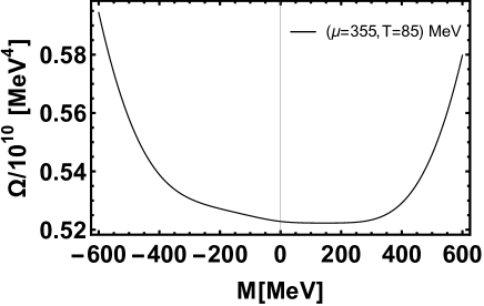
Figure 5: Behavior of Contact Interaction effective Potential at the critical end point.

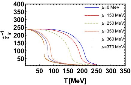
(a)

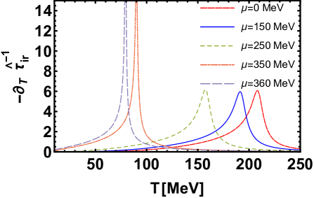
(b)

Figure 6: (6(a)) Behavior of the confining length scale as a function of temperature for various values of the chemical potential $\mu$. (6(b)) Thermal gradient of the confining scale as a function of temperature for various values of the chemical potential.

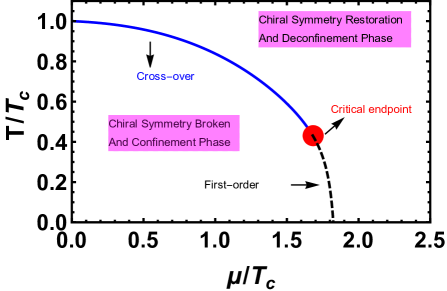
Figure 7: QCD phase diagram in $T-\mu$ plane: the black solid line represents the cross-over phase transition while the red-dashed line represents the first order phase transition. The red-dot represent the critical endpoint

We further consider the screening effects of the medium which dilute the strength of the effective coupling are by including the vacuum polarization contribution due to quarks at high temperatures into the framework with slight modification in Eq. (6) as [72]

$$\alpha^{N_{c}}_{\rm eff}(N_{f},T)=\frac{\alpha^{N_{c}}_{\rm eff}(N_{f})}{1+\frac{\alpha^{N_{c}}_{\rm eff}(N_{f})T^{2}}{3}}.$$ (23)

With this modification, we obtain the critical temperature $T_{c}\approx 132$ MeV at $\mu=0$, which shows the effect of the medium in diluting the coupling. At $T=0$, $\mu_{c}\approx 380$ MeV. For the CEP, the model yields $T_{E}\approx 65$ MeV and $\mu_{E}\approx 340$ MeV such that ($T^{E}_{c}/T_{c}\approx 0.57,~{}\mu^{E}_{c}/T_{c}\approx 2.6$) in the phase diagram, as shown in Fig. 8.

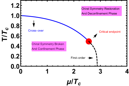
Figure 8: QCD phase diagram in $T-\mu$ plane: Coupling constant with screening effects of the medium, Eq. (23).

In the next section, we summarize our findings and draw the conclusions.

4 Summary and Conclusions

In the present manuscript we have studied the dynamical chiral symmetry breaking/restoration and confinement-deconfinement phase transitions at finite temperature $T$ and chemical potential $\mu$ and sketched the QCD Phase diagram in the $T-\mu$ plane. We used a flavor dependent symmetry preserving vector-vector confining contact interaction model of quarks and Schwinger optimal proper time regularization scheme. We have developed an expression for effective thermodynamic potential and identify the signals of chiral symmetry breaking-restoration from the peaks of the thermal gradient of the dynamical mass. The confinement-deconfinement transition is pinpointed from the peaks of the thermal gradient of the confining scale at various quark chemical potential. At finite temperature $T$ and $\mu=0$, our analysis shows that the chiral symmetry is restored and deconfinement occurs when $T$ reaches a critical value $T_{c}\approx 208$ MeV and the order of the transition is a cross-over. In the presence of quark chemical potential $\mu$ and $T=0$, the dynamical chiral symmetry is restored and deconfinement occurs when $\mu$ exceeds its critical value $\mu_{c}\approx 350$ MeV. At the end, we have sketched the phase diagram in the $T-\mu$ plane. Our results in this scenario show that the cross-over transition line in the phase diagram started from the finite $T$-axis continued along the finite $\mu$-axis until the CEP $(\mu^{E}_{c}/T_{c}\approx 1.6$, $T^{E}_{c}/T_{c}\approx 0.43)$ where above, the transition changes to the first-order till at $T=0$ along $\mu$-axis. It should be noted that the exact location of the CEP is not yet exactly known. However some effective model calculations  [40, 41, 42, 43, 44, 45, 46, 23, 25, 38], Schwinger-Dyson equations [21, 22, 23, 24, 25, 26, 27, 28, 29, 30, 31] and mathematical extensions of lattice techniques  [47, 48, 49, 50] set the range between $(\mu_{E}/T_{c}=1.0-2.0,T_{E}/T_{c}=0.4-0.9)$. When considering screening effects of the medium, which dilute the strength of the effective coupling, by including the vacuum polarization contribution due to quarks at high temperatures, it yields the location of the CEP at $(\mu^{E}_{c}/T_{c}\approx 2.6,T^{E}_{c}/T_{c}\approx 0.57)$, which hints for a deeper analysis of screening effects on models of this kind, which is currently been carried out. In the near future, we also plan to extend this work to study the electromagnetic effects and other areas of the hot and dense QCD, the light hadrons properties under extreme conditions etc., using the contact interaction model.

References

References

- [1] Gross D J and Wilczek F 1973 Phys. Rev. Lett. 30 1343–1346
- [2] Politzer H D 1973 Phys. Rev. Lett. 30 1346–1349
- [3] Wilson K G 1974 Phys. Rev. D 10 2445–2459
- [4] Rischke D, Friman B, Stocker H and Greiner W 1988 Journal of Physics G: Nuclear Physics 14 191
- [5] McLerran L and Pisarski R D 2007 Nuclear Physics A 796 83–100
- [6] McLerran L 2009 Nuclear Physics A 830 709c–712c
- [7] Shao G y 2011 Physics Letters B 704 343–346
- [8] Barrois B C 1977 Nucl. Phys. B 129 390–396
- [9] Casalbuoni R and Gatto R 1999 Phys. Lett. B 469 213–219 (Preprint hep-ph/9909419)
- [10] Rajagopal K 1999 Nucl. Phys. A 661 150–161 (Preprint hep-ph/9908360)
- [11] Arslandok M et al. 2023 (Preprint 2303.17254)
- [12] Durante M, Indelicato P, Jonson B, Koch V, Langanke K, Meißner U G, Nappi E, Nilsson T, Stöhlker T, Widmann E et al. 2019 Physica Scripta 94 033001
- [13] Kolesnikov V I, Kekelidze V D, Matveev V A and Sorin A S 2020 Phys. Scripta 95 094001
- [14] Aoki Y, Endrodi G, Fodor Z, Katz S D and Szabo K K 2006 Nature 443 675–678 (Preprint hep-lat/0611014)
- [15] Cheng M et al. 2006 Phys. Rev. D 74 054507 (Preprint hep-lat/0608013)
- [16] Bhattacharya T et al. 2014 Phys. Rev. Lett. 113 082001 (Preprint 1402.5175)
- [17] de Forcrand P, Langelage J, Philipsen O and Unger W 2014 Phys. Rev. Lett. 113 152002 (Preprint 1406.4397)
- [18] Bazavov A et al. (HotQCD) 2019 Phys. Lett. B 795 15–21 (Preprint 1812.08235)
- [19] Borsanyi S, Fodor Z, Guenther J N, Kara R, Katz S D, Parotto P, Pasztor A, Ratti C and Szabo K K 2020 Phys. Rev. Lett. 125 052001 (Preprint 2002.02821)
- [20] Guenther J N 2021 Eur. Phys. J. A 57 136 (Preprint 2010.15503)
- [21] Qin S x, Chang L, Chen H, Liu Y x and Roberts C D 2011 Phys. Rev. Lett. 106 172301 (Preprint 1011.2876)
- [22] Fischer C S, Luecker J and Mueller J A 2011 Phys. Lett. B 702 438–441 (Preprint 1104.1564)
- [23] Gutiérrez E, Ahmad A, Ayala A, Bashir A and Raya A 2014 Journal of Physics G: Nuclear and Particle Physics 41 075002
- [24] Eichmann G, Fischer C S and Welzbacher C A 2016 Phys. Rev. D 93 034013 (Preprint 1509.02082)
- [25] Ahmad A, Ayala A, Bashir A, Gutiérrez E and Raya A 2015 J. Phys. Conf. Ser. 651 012018
- [26] Gao F and Liu Y x 2016 Phys. Rev. D 94 076009 (Preprint 1607.01675)
- [27] Ahmad A and Raya A 2016 Journal of Physics G: Nuclear and Particle Physics 43 065002
- [28] Fischer C S 2019 Prog. Part. Nucl. Phys. 105 1–60 (Preprint 1810.12938)
- [29] Shi C, He X T, Jia W B, Wang Q W, Xu S S and Zong H S 2020 JHEP 06 122 (Preprint 2004.09918)
- [30] Ahmad A 2021 Chin. Phys. C 45 073109 (Preprint 2009.09482)
- [31] Ahmad A, Bashir A, Bedolla M A and Cobos-Martínez J J 2021 J. Phys. G 48 075002 (Preprint 2008.03847)
- [32] Klevansky S 1992 Reviews of Modern Physics 64 649
- [33] Buballa M 2005 Physics Reports 407 205–376
- [34] Costa P, Ruivo M C, De Sousa C A and Hansen H 2010 Symmetry 2 1338–1374
- [35] Marquez F, Ahmad A, Buballa M and Raya A 2015 Physics Letters B 747 529–535
- [36] Ayala A, Flores J A, Hernandez L A and Hernandez-Ortiz S 2018 EPJ Web Conf. 172 02003 (Preprint 1712.00187)
- [37] Ayala A, Hernández L A, Loewe M and Villavicencio C 2021 Eur. Phys. J. A 57 234 (Preprint 2104.05854)
- [38] Ahmad A and Murad A 2022 Chin. Phys. C 46 083109 (Preprint 2201.09980)
- [39] Nishi T, Itahashi K, Ahn D, Berg G P, Dozono M, Etoh D, Fujioka H, Fukuda N, Fukunishi N, Geissel H et al. 2023 Nature Physics 1–6
- [40] Sasaki C, Friman B and Redlich K 2008 Phys. Rev. D 77 034024 (Preprint 0712.2761)
- [41] Costa P, Ruivo M C and de Sousa C A 2008 Phys. Rev. D 77 096001 (Preprint 0801.3417)
- [42] Fu W j, Zhang Z and Liu Y x 2008 Phys. Rev. D 77 014006 (Preprint 0711.0154)
- [43] Abuki H, Anglani R, Gatto R, Nardulli G and Ruggieri M 2008 Phys. Rev. D 78 034034 (Preprint 0805.1509)
- [44] Loewe M, Marquez F and Villavicencio C 2013 Phys. Rev. D 88 056004 (Preprint 1307.6764)
- [45] Kovacs P and Szep Z 2008 Phys. Rev. D 77 065016 (Preprint 0710.1563)
- [46] Schaefer B J, Pawlowski J M and Wambach J 2007 Phys. Rev. D 76 074023 (Preprint 0704.3234)
- [47] Fodor Z and Katz S D 2002 Journal of High Energy Physics 2002 014
- [48] Gavai R V and Gupta S 2005 Physical Review D 71 114014
- [49] Li A, Alexandru A, Meng X, Liu K F, QCD Collaboration et al. 2009 Nuclear Physics A 830 633c–635c
- [50] de Forcrand P and Kratochvila S 2006 Nucl. Phys. B Proc. Suppl. 153 62–67 (Preprint hep-lat/0602024)
- [51] Ruggieri M and Peng G X 2016 Phys. Rev. D 93 094021 (Preprint 1602.08994)
- [52] Bali G S, Bruckmann F, Endrodi G, Fodor Z, Katz S D, Krieg S, Schafer A and Szabo K K 2011 PoS LATTICE2011 192 (Preprint 1111.5155)
- [53] Tavares W R, Farias R L S and Avancini S S 2020 Phys. Rev. D 101 016017 (Preprint 1912.00305)
- [54] Wang L and Cao G 2018 Phys. Rev. D 97 034014 (Preprint 1712.09780)
- [55] Nambu Y and Jona-Lasinio G 1961 Physical Review 124 246
- [56] Ebert D, Feldmann T and Reinhardt H 1996 Phys. Lett. B388 154–160 (Preprint hep-ph/9608223)
- [57] Gutierrez-Guerrero L X, Bashir A, Cloet I C and Roberts C D 2010 Phys. Rev. C81 065202 (Preprint 1002.1968)
- [58] Roberts H L L, Roberts C D, Bashir A, Gutierrez-Guerrero L X and Tandy P C 2010 Phys. Rev. C82 065202 (Preprint 1009.0067)
- [59] Roberts H L L, Bashir A, Gutierrez-Guerrero L X, Roberts C D and Wilson D J 2011 Phys. Rev. C83 065206 (Preprint 1102.4376)
- [60] Roberts H L L, Chang L, Cloet I C and Roberts C D 2011 Few Body Syst. 51 1–25 (Preprint 1101.4244)
- [61] Wang K l, Liu Y x, Chang L, Roberts C D and Schmidt S M 2013 Phys. Rev. D87 074038 (Preprint 1301.6762)
- [62] Ahmad A and Raya A 2016 J. Phys. G43 065002 (Preprint 1602.06448)
- [63] Ahmad A and Farooq A 2023 (Preprint 2302.13265)
- [64] Marquez F, Ahmad A, Buballa M and Raya A 2015 Phys. Lett. B747 529–535 (Preprint 1504.06730)
- [65] Langfeld K, Kettner C and Reinhardt H 1996 Nucl. Phys. A 608 331–355 (Preprint hep-ph/9603264)
- [66] Cornwall J M 1982 Phys. Rev. D 26 1453
- [67] Aguilar A C, Binosi D and Papavassiliou J 2016 Front. Phys. (Beijing) 11 111203 (Preprint 1511.08361)
- [68] Kohyama H 2016 (Preprint 1602.09056)
- [69] Boucaud P, Leroy J P, Yaouanc A L, Micheli J, Pene O and Rodriguez-Quintero J 2012 Few Body Syst. 53 387–436 (Preprint 1109.1936)
- [70] Solis E L, Costa C S R, Luiz V V and Krein G 2019 Few Body Syst. 60 49 (Preprint 1905.08710)
- [71] Ahmad A, Martínez A and Raya A 2018 Phys. Rev. D 98 054027 (Preprint 1809.05545)
- [72] Lo P M, Szymański M, Redlich K and Sasaki C 2022 The European Physical Journal A 58 172 ISSN 1434-601X URL https://doi.org/10.1140/epja/s10050-022-00822-7