Design and Control of a Bio-inspired Wheeled Bipedal Robot

Abstract

Wheeled bipedal robots (WBRs) have the capability to execute agile and versatile locomotion tasks. This paper focuses on improving the dynamic performance of WBRs through innovations in both hardware and software aspects. A bio-inspired mechanical design, inspired by the human barbell squat, is proposed and implemented, as is shown in Fig. 1, such design aims to distribute the torque load onto the hip and knee joints, imitating the bio-mechanics of human squatting and improving efficiency of all motors, while the base workspace is still maintained large. Meanwhile, a novel model-based controller is devised, which synthesizes wheeled linear inverted pendulum (wLIP) model, Control Lyapunov Function (CLF) and whole-body dynamics for theoretically guaranteed stability and efficient computation. The wLIP surpasses other alternatives in terms of agility by providing a more accurate approximation of wheeled-bipedal locomotion. Experimental results demonstrate that the robot could perform human-like deep squat motion, and is capable of maintaining balance while manipulating base states and CoM velocity; furthermore, it exhibits robustness against external disturbances and unknown terrains.

I Introduction

Wheeled bipedal robots (WBRs) [1, 2] integrates both the advantages of low-cost transportation of wheeled robots and the high trafficability of legged robots. However, after the development in recent years, the design and control of wheeled bipedal robots are still primitive compared with the booming development of legged bipedal robots. In the following sections, we will introduce the recent development of WBRs in terms of mechanical design and relevant control algorithms.

I-A Mechanical Design

The most well-known WBR is the Ascento [1], developed by ETH research in 2019. The design of Ascento includes a pair of four-bar linkage legs, each leg is with 1 degree of freedom (DoF) and equipped with the torsional springs in the knee joint to alleviate impacts. It can jump upstairs or lower down its head to pass obstacles while balancing on wheels. However, its usage is highly limited for complex tasks due to the lack of sufficient DoFs in leg.

Recently, WBRs with 2 DoF legs emerged, adding the ability to control the base height and orientation simultaneously on top of the capability of Ascento. Similar to the design of robotic manipulators such as delta robots [3] or serial robotic arms [4], the design of WBR legs with 2 DoFs also involves the trade-off between workspace and load capability. A five-bar linkage parallel layout, as is shown in Fig.2a, distributes the weight evenly onto the two symmetrically installed motors to increase load capacity, such as the Tencent Ollie [2]. However, the parallel mechanism limits the workspace of the base links, e.g., operational height and base pitch angle.

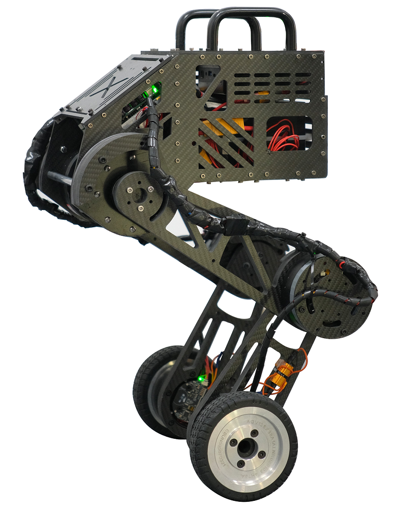
Figure 1: Overview of the bio-inspired wheeled bipedal robot.

On the contrary, WBRs with planar two-link serial legs [5, 6, 7, 8, 9, 10], shown in Fig. 2b, have larger workspace compared to the five-bar linkage design. The planar two-link design is often similar to the quadrupedal robot MIT Mini-Cheetah [11], of which the central axis of the knee joint motor and the hip joint are aligned and placed close to the upper body to reduce the leg inertia. However, this adaptation to bipedal robots exhibits low efficiency in terms of joint torques: for such a WBR in the double support phase, the moment arm of knees are much longer than that of the hips, consequently, the majority of the weight is supported by the knee motors, leading to the rapid heat accumulation in knee motors. In contrast, the hip motors contribute much lower torque to support the self-weight of WBRs. The difference in torque distribution across hip and knee motors can be extremely high, wasting of the hip joint motors and challenging the operation of knee joint motors. In summary, the mechanical design of WBRs with 2 DoF legs mainly involves the trade-off between flexible workspace and proper load distribution in knee and hip joints.

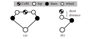
Figure 2: Schematic demonstration of WBRs with 2 DoF legs. (a): five-bar linkage. (b): planar 2-link serial layout. The dashed line represents the short distance between the CoM and the hip joint, leading to the much longer momentum arm for the knee joint motors.

I-B Controller Design

Due to the instability nature of WBRs, the controller designed for WBRs are mostly model-based: a dynamic model is required to compute the controllers, and the resulting performance depends on the model precision. The model-based controllers for WBRs starts from a popular model, wheeled inverted pendulum (WIP) [12]. The WIP model approximates the WBRs with a inverted pendulum with wheels in the foot, length of the pendulum is assumed to be constant, making the model easy to use in numerical computation. The WIP model is integrated with PID controllers [8, 1, 10, 2], whole body controllers (WBC) [6, 13, 9, 5], and model predictive controllers (MPC) [7, 14] for various scenarios and applications. However, for WBRs with 2 DoFs legs to simultaneously control the height and orientation, the assumption of constant leg length will be inevitably violated, leading to the performance degradation in model-based controllers.

Recent works on controlling WBRs with 2 DoFs legs have proposed new models with higher DoFs to overcome the simplicity of WIP. For instance, a nonlinear wheeled spring-loaded inverted pendulum model (W-SLIP) [5] is developed from the bipedal walking theory to improve the performance of nonlinear trajectory optimization, but is inapplicable to real-time control due to its complex nonlinear formulation. A Cart-Linear-Inverted-Pendulum-Model (Cart-LIPM) [15] is adapted from the linear inverted pendulum (LIP), the linearity of Cart-LIPM enables real-time trajectory optimization (TO) with MPC and the optimized trajectory is tracked by WBC. However, the ignorance of wheel torque prevents its application in real-world experiments. Recently, the single rigid body model is adapted to its wheeled version (WRBD) for WBR [7], MPC is employed to online compute the wheel trajectory and reaction forces to manipulate the base velocity and posture, and then tracked by WBC. The main barrier for application of WRBD is its high nonlinearity and the resulting computational burden by using iterative dynamic programming. Furthermore, common to all the above mentioned control algorithms is that, while the control stability is essential to WBR systems, all the previous works lack the rigorous analysis in control stability, limiting the generality of the proposed algorithms.

Besides the model-based control methods, there are works that utilizes reinforcement learning (RL) methods to control the WBRs [16, 17, 18]. The RL methods often requires the exploration process to collect sufficient training data for learning the control policy, but due to the instability essence of WBRs, exploration with hardware system is often inapplicable. Consequently, applying RL methods in WBRs could only collect data and learning control policy with the imprecise model in simulation, the inevitable model-bias makes it non-trivial to implement the learned policy in hardware experiments [19].

I-C Contributions

In this paper, we propose a bio-inspired WBR with an efficient online controller. The bio-inspired mechanical design could improve the performance of load-carrying squat, which shares similarities to a wide range of challenging tasks in robots with bipedal structures [20]. Inspired by human deep squats, its bionic design captures the underlying principle of efficient squats and imitates the human mass layout. The proposed controller integrates a novel wheeled LIP (wLIP) model with improve model precision and guaranteed stability. The new wLIP model extends the Cart-LIPM [15] by incorporating the wheel torques; meanwhile, the proposed control method includes a balancing controller based on Control Lyapunov Function (CLF) [21, 22] to ensure the asymptotic stability of the centroidal self-balancing dynamics. Advantages of the proposed mechanical design and controllers are demonstrated with comprehensive simulations and hardware experiments.

The primary contributions could be summarized as:

I-C1 Mechanical Design

We proposed a novel bio-inspired WBR design, the design overcomes the low torque efficiency flaw of previous works on serial-legged WBR but also maintains its mechanical size to ensure large workspace property.

I-C2 Controller

We propose a novel model-based controller based on the WBC structure. The proposed controller (i) includes the new wLIP model, considering the wheel torque and variable leg length, to improve the control performance while the linear structure maintains the computational efficiency; (ii) integrates WBC with the CLF-based stability condition and the wLIP model to enable velocity and posture manipulation, guarantee real-time stability and control performance.

The paper is structured as follows: In Section II, we introduce the bio-inspired wheeled-bipedal robot design and the full model dynamics and kinematics. In Section III, we introduce the wLIP model and we propose the CLF-wLIP condition to guaranteed stability. In Section IV, we propose an efficient tracking controller for the WBR system with weighted QP structure. In Section V, we demonstrate the advantages of wLIP model, verify the static and dynamic performance, and the robustness against disturbance of the proposed weighted QP controller. In Section VI, we conclude this paper.

II Bio-inspired Mechanical Design

In this paper, we aim to design a bio-inspired WBR with improved squat performance with load. Typically when designing the leg and mass layout of WBR with 3-link planar structure, the design could be formulated as a nonlinear programming (NLP) problem, where the leg lengths and the mass distribution could be defined as free variables and the minimization of operation torques or mechanical power could be defined as the objective function [23]. However, the derived NLP is often sensitive to parameter setting, e.g., the height bounds and the weights of torques, and is often limited to specific scenarios like stance or running [23, 24], indicating oversimplification and lacking universality. Meanwhile, the squat serves as one of the most commonly used motions in athletic and everyday activities [25]; similarly, the squatting motion serves as the basis of many explosive tasks like load lifting and jumping, which are non-trivial to WBR systems. Inspired by the fact that the human bio-mechanics naturally solves the leg design problem in normal life, we desire to obtain a suitable WBR design by imitating human bio-mechanics and maintain characteristics of human leg motion, a typical barbell squat exercise process is shown in Fig. 3a.

II-A Link Length Design

The link length ratios of our proposed WBR robot are designed to imitate the human torso-thigh-shank ratio. According to the previous result in human bio-mechanics research on powerlifting [26], the shank length $l_{k}$ is approximately 80% of the thigh $l_{h}$, and the upper body hip-to-CoM length $l_{p}$ (without head, assuming quasi-uniform mass distribution) is about 60% of the thigh $l_{h}$. Consequently, ratio of the leg length of the wheeled-bipedal robot could be similarly defined as

$$[l_{p}:l_{h}:l_{k}]=[3:5:4].$$ (1)

Considering the bio-inspired leg length ratio (1) and engineering practice, we select $l_{p}=150$mm, $l_{h}=250$mm, $l_{k}=200$mm.

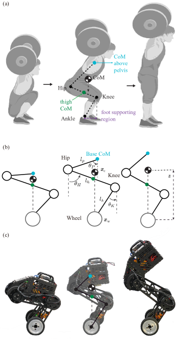
Figure 3: Bionic design of the wheeled-bipedal robot. (a) The squatting process with load of human. (b) The simplified design model imitating human squatting. (c) The hardware implementation of the bionic WBR in squatting process, the bionic design enables the WBR to perform human-like squat trajectories. Parameter $z$ is the body CoM height from the wheel center and $x_{c}$, $x_{w}$ are respectively the body CoM and wheel horizontal positions in sagittal plane. $l_{p}$, $l_{h}$, $l_{k}$ are respectively the link length of the base, thigh, and shank.

II-B Mass & Torque Distribution

After selecting the leg length, we note that the mass distribution of human leg is different from the commonly used WBR design in Fig. 2b: the previous designs concentrate the weight at hip; while such design eases the modeling by assuming the leg is massless, the knee joint is required to support nearly all the load, which leads to rapid overheating of the knee joint motor and limits the load capability. However, in human bio-mechanics, human leg distributes the weight across hip and knee muscles[27]. It is also reported that during explosive leg motion such as squatting and jumping, the work done by the hip and knee muscles are approximately the same [28, 29]. As illustrated in Fig. 3a, when humans attempt to lift a heavy barbell, they will actively change their posture to control the moment arm of each joint to distribute the load onto different muscles. Motivated by these studies, we installed the auxiliary components, e.g., batteries, on the base, and arranged the hip and knee motors at the hip and knee joints to imitate the heavy human thigh muscles, as shown in Fig. 3b. Furthermore, to balance the work done by the hip and knee joint motors, we introduce the torque ratio

$$r_{\tau}=\bigg{|}\frac{\tau_{h}}{\tau_{k}}\bigg{|},$$ (2)

where $\tau_{h},\tau_{k}$ are hip and knee joint torques, absolute value aims to eliminate the potential influence of different torque direction. For ease of design, we select the same type of motors , they have the same rated output capability. Consequently, during the squat motion, we aim to control the $r_{\tau}$ around 1 to fully utilize their strength and maximize the load capacity. It can be implemented by controlling the moment arm of the load supported by each joint, similar to humans performing deep squats. To the best of our knowledge, there have been many successfully implemented wheeled bipedal robots while none has explicitly considered this from the aspect of bionic inspiration.

In summary, inspired by the bio-mechanics of human leg, we designed the leg length with specific ratio, rearranged the hip and knee motors at the corresponding joints, and proposed the key principle for improving stance load capability: optimize the torque ratio $r_{\tau}$ around 1 by regulating the joint moment arms. The proposed mechanical design and squat process is presented in Fig. 3c while the summarized control principles will be detailed and demonstrated in Section V. In the remainder of this section, we will derive a general whole body dynamic model for the proposed WBR.

II-C Dynamic Model

The proposed WBR shown in Fig. 3c has 6 actuated DoFs (joints and wheels for two legs) $\mathbf{q}_{j}\in\mathbb{R}^{6}$ and 6 floating DoFs, i.e., XYZ translation $\mathbf{r}_{\text{xyz}}\in\mathbb{R}^{3}$ and Euler ZYX rotation: yaw $\phi\in\mathbb{R}$, pitch $\theta\in\mathbb{R}$, roll $\psi\in\mathbb{R}$. Note that in this project, we use Featherstone’s spatial algebra notation [30]. Let $\mathbf{q}=[\mathbf{r}_{xyz},\phi,\theta,\psi,\mathbf{q}_{j}]^{\top}\in\mathbb{R}^{12}$, the robot dynamics can be expressed in the following equation of motion (EoM):

$$\mathbf{M}(\mathbf{q})\ddot{\mathbf{q}}+\mathbf{H}(\mathbf{q},\dot{\mathbf{q}}) =\mathbf{S}\boldsymbol{\tau}+{}_{C}\mathbf{J}^{\top}_{c}{}_{C}\mathbf{F}_{c},$$ (3a)

$${}_{W}\mathbf{J}_{c}\ddot{\mathbf{q}}+{}_{W}\dot{\mathbf{J}}_{c}\dot{\mathbf{q}} =\mathbf{C}_{r},$$ (3b)

where $\mathbf{M}\in\mathbb{R}^{12\times 12}$ is the joint space inertia matrix (JSIM), $\mathbf{H}\in\mathbb{R}^{12}$ is the nonlinear effect including the Coriolis force and gravitational force, $\mathbf{S}=[\mathbf{0}_{6\times 6}\quad\mathbf{I}_{6}]$ is the selection matrix, ${}_{W}\mathbf{J}_{c},{}_{C}\mathbf{J}_{c}\in\mathbb{R}^{6\times 12}$ are respectively the contact Jacobian matrices expressed in $\{W\}$ and $\{C\}$ of the two wheels, ${}_{C}\mathbf{F}_{c}=[\mathbf{f}_{c}^{\text{left}},\mathbf{f}_{c}^{\text{right}}]\in\mathbb{R}^{6}$ is the vector of the linear contact forces exerted on $c$, and $\mathbf{C}_{r}\in\mathbb{R}^{6}$ is the rolling constraint defined later. Details of the contact frames are illustrated in Fig. 4.

Rolling Constraints

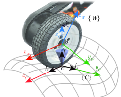
Figure 4: Contact frame illustration of the right wheel. $\{C\}$ has its z-axis normal to the ground, its x-axis opposite the floating-base x-axis, and its origin at the contact point $c$. $\{W\}$ is rotated from $\{C\}$ by clockwise angle $\psi$ w.r.t. $x_{C}$ and has its origin at the wheel center $o$. The transparent blue cone represents the friction cone constraint of the 3D linear force components $\mathbf{f}_{c}^{(\cdot)}=[f_{x},f_{y},f_{z}]$ where $(\cdot)$ can be left or right.

To estimate the base linear velocity $\dot{\mathbf{r}}_{xyz}$ and enable control based on inverse dynamics (ID), we need to utilize the contact constraints. Let $\boldsymbol{\omega}_{o}\in\mathbb{R}^{3}$ be the wheel angular velocity expressed in $\{W\}$. The rolling kinematic constraint refers to maintaining the linear velocity of the contact point $c$ as zero, i.e.,

$${}_{W}\mathbf{v}_{c}=\begin{bmatrix}\boldsymbol{\omega}_{o}\\ \mathbf{0}_{3\times 1}\end{bmatrix}=\begin{bmatrix}\mathbf{I}_{3}&\mathbf{0}_{3\times 3}\\ -{}_{W}\mathbf{r}_{c}\times&\mathbf{I}_{3}\end{bmatrix}\begin{bmatrix}\boldsymbol{\omega}_{o}\\ {}_{W}\boldsymbol{v}_{o}\end{bmatrix}$$ (4)

where $o$ is the wheel center, ${}_{W}\textbf{r}_{c}=[0,0,-r_{w}]$ is the contact point position and $r_{w}$ is the wheel radius. By differentiating the linear velocity part in (4) with respect to time, we have

$$\mathbf{0}_{3\times 1}=-{}_{W}\mathbf{r}_{c}\times\dot{\boldsymbol{\omega}}_{o}+{}_{W}\dot{\boldsymbol{v}}_{o}.$$ (5)

Let $\sigma$ be the counterclockwise angle between the x-axis of $\{W\}$ and the position vector of any point $p_{\sigma}$ on the wheel contour. The spatial acceleration of $p_{\sigma}$ parameterized by $\sigma$ expressed in $\{W\}$ is

$${}_{W}\dot{\mathbf{v}}_{p_{\sigma}}=\begin{bmatrix}\dot{\boldsymbol{\omega}}_{o}\\ {}_{W}\dot{\boldsymbol{v}}_{p_{\sigma}}\end{bmatrix}=\left[\begin{array}[]{c}\dot{\boldsymbol{\omega}}_{o}\\ -\dot{\mathbf{r}}(\sigma)\times\boldsymbol{\omega}_{o}-\mathbf{r}(\sigma)\times\dot{\boldsymbol{\omega}}_{o}+\dot{{}_{W}\boldsymbol{v}}_{o}\end{array}\right],$$ (6)

where $\mathbf{r}(\sigma)=[r_{w}\cos\sigma,0,r_{w}\sin\sigma]^{\top}\in\mathbb{R}^{3}$ is the displacement from the wheel center to the point. For the contact point $c=p_{\pi/2}$, $\sigma=\pi/2,\mathbf{r}(\sigma)={}_{W}\textbf{r}_{c}$. Considering that $\dot{\mathbf{r}}(\sigma)=[-r_{w}\dot{\sigma}\sin\sigma,0,r_{w}\dot{\sigma}\cos\sigma]^{\top}$, substituting (5) into (6) gives

$$\begin{aligned} {}_{W}\dot{\boldsymbol{v}}_{c}=-\dot{\mathbf{r}}(\pi/2)\times\boldsymbol{\omega}_{o}=\left[\begin{array}[]{c}0\\ -r_{w}\dot{\sigma}\omega_{oz}\\ r_{w}\dot{\sigma}\omega_{oy}\end{array}\right]\in\mathbb{R}^{3}\end{aligned},$$ (7)

where $\dot{\sigma}$ is the time derivative of the wheel pitch angle, and the $\omega_{oz},\omega_{oy}$ are the $z,y$ components of $\boldsymbol{\omega}_{o}$, which can easily be calculated using Pinocchio [31]. Consequently, the rolling constraint $\mathbf{C}_{r}$ in (3b) is defined as

$$\mathbf{C}_{r}=[{}_{W}\dot{\boldsymbol{v}}_{c,\text{left}}^{\top},{}_{W}\dot{\boldsymbol{v}}_{c,\text{right}}^{\top}]^{\top}.$$ (8)

Linearized Friction Cone

To avoid slippage of wheels and consequent failure in contact-aided state estimation, friction cone constraint is often added, i.e.,

$$\forall\mathbf{f}_{c}^{(\cdot)}\in{}_{C}\mathbf{F}_{c},\;f_{z}^{(\cdot)}\geq 0,\;\sqrt{[f_{x}^{(\cdot)}]^{2}+[f_{y}^{(\cdot)}]^{2}}<\mu f_{z}^{(\cdot)},$$ (9)

where ^(⋅) can be left or right, and $\mu$ is the friction coefficient. In common WBC implemtation [40, 13], the friction cone constraint is usually linearized to be incorporated into the QP framework:

$$\forall\mathbf{f}_{c}^{(\cdot)}\in{}_{C}\mathbf{F}_{c},\;f_{z}^{(\cdot)}\geq 0,\;|f_{x}^{(\cdot)}|<\mu f_{z}^{(\cdot)},\;|f_{y}^{(\cdot)}|<\mu f_{z}^{(\cdot)}.$$ (10)

III Wheeled Linear Inverted Pendulum model

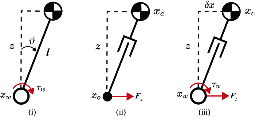
Figure 5: Simplified model illustration. (i) WIP (ii) LIP (iii) wLIP.

Due to the unstable essence of WBR system, the controllers applied in WBR are usually divided into two layers: the upper layer is model-based planner for motion planning, the lower layer tracks the planned trajectory generated from upper layer. As the complete dynamic model for WBR,(3) is too complex to ensure real-time planning, a simplified model is usually required for efficient computation while ensuring sufficiently precise modeling. In this section we will propose a new simplified model with improved modeling precision compared to commonly used WIP model [12], and present the stability condition for the proposed WBR with wLIP model. A schematic presentation of the related models are shown in Fig. 5. We note that throughout this paper, the term body refers to the parts excluding the wheels. For simplicity, we will use CoM to refer to the body CoM and CAM to refer to the body CAM.

III-A The WIP Model

We first recall the WIP model as the base line for comparison. The wheeled inverted pendulum (WIP) model [12] as shown in Fig. 5i is widely used for two-wheeled robot control. One can derive the EoM of WIP using the Euler-Lagrange Equation as

$$\begin{bmatrix}I_{c}+m_{c}l^{2}&m_{c}l\cos\vartheta\\ m_{c}lr_{w}\cos\vartheta&\frac{I_{w}+(m_{w}+m_{c})r_{w}^{2}}{r_{w}}\end{bmatrix}\begin{bmatrix}\ddot{\vartheta}\\ \ddot{x}_{w}\end{bmatrix}$$ (11)

$$\;\;\;\;\;\;\;\;\;\;\;\;\;\;\;\;\;\;\;\;\;\;\;\;\;\;\;-m_{c}l\sin\vartheta\begin{bmatrix}g\\ r\dot{\vartheta}^{2}\end{bmatrix}=\tau_{w}\begin{bmatrix}-1\\ 1\end{bmatrix},$$

where $g$ is the gravity acceleration, $l$ is the distance between the CoM and the wheel center, $r_{w}$ is the wheel radius, $I_{w}$ is the wheel centroidal inertia, $I_{c}$ is the body centroidal inertia, $\tau_{w}$ is the wheel torque, $x_{w}$ is the wheel center position, and $\vartheta$ is the clockwise CoM angle between the gravity and the body-wheel linkage. $m_{c}$ is the body mass and $m_{w}$ is the wheel mass. It is clearly shown in (11) that the WIP model assumes constant leg length $l$ and has nonlinear dynamics due to the direct coupling between CoM with the wheels, leading to the imprecise modeling in WBR and the computational complexity when implementing real-time controller.

III-B The wLIP Model

We first recap the Linear Inverted Pendulum (LIP) model as shown in Fig. 5ii, it is a well-studied reduced-order model of bipedal robot walking [32]. It constrains the CoM height to be constant and that the centroidal torque should be zero to ensure zero centroidal angular momentum (CAM), i.e.,

$$F_{x}=m_{c}g\frac{x_{c}-x_{0}}{z},$$ (12)

where $F_{x}$ is the horizontal component of the ground reaction force (GRF), $m_{c}$ is the body mass, $z$ is the CoM height, $x_{c}$ is the CoM horizontal position, and $x_{0}$ is the stance foot location. Therefore, the CoM planar dynamics is

$$\ddot{x}_{c}=\frac{g}{z}(x_{c}-x_{0}).$$ (13)

The LIP, named after its linearity, significantly facilities the controller design and stability analysis of walking robots, while the leg length is considered variable to provide improve modeling precision. However, as the model does not consider wheeled foot, it could not be applied directly to our WBR system.

To adapt the idea of LIP to wheeled bipedal robots, we first recognize that the interaction force replaces the $F_{x}$ at the wheel-leg connection and that the wheeled model does not switch stance foot. Assuming that the body behaves similarly to the LIP, i.e., constant CoM height and zero CAM, we have the reduced order model for wheeled bipedal robots, the wheeled linear inverted pendulum (wLIP) as shown in Fig. 5iii as

$$zF_{t}+\tau_{w}=m_{c}g(x_{c}-x_{w}),$$ (14)

$$\frac{\tau_{w}}{r_{w}}-F_{t}=m_{w}\ddot{x}_{w},$$

where $F_{t}$ is the horizontal interactive force between the body and the wheel. Let $\delta x=x_{c}-x_{w}$, the above linear equations can be rewritten in state-space form:

$$\begin{bmatrix}\ddot{x}_{c}\\ \delta\ddot{x}\\ \delta\dot{x}\end{bmatrix}= \underbrace{\begin{bmatrix}0&0&\frac{g}{z}\\ 0&0&(1+\frac{m_{c}}{m_{w}})\frac{g}{z}\\ 0&1&0\end{bmatrix}}_{\mathbf{A}(z)}\begin{bmatrix}\dot{x}_{c}\\ \delta\dot{x}\\ {\delta x}\end{bmatrix}$$ (15)

$$+\underbrace{\begin{bmatrix}\frac{1}{m_{c}z}\\ -(\frac{1}{m_{c}}+\frac{1}{m_{w}})\frac{1}{z}-\frac{1}{m_{w}r_{w}}\\ 0\end{bmatrix}}_{\mathbf{B}(z)}\tau_{w}.$$

It is easy to analyze with this symbolic form that the wLIP dynamics is controllable. Since no stance foot switch is required, the wLIP is continuous everywhere, making it easier to analyze than the LIP model.

Remark 1 (Superiority of wLIP).

Due to the nonlinearity of WIP in (11), normally the WIP is linearized around $\vartheta=0$, and a linear controller such as LQR is used to regulate $\vartheta$. For example, Ascento uses a set of sampled $l$ to calculate an LQR gain library and interpolates within it using the real-time $l$ feedback [13], leading to imprecise modeling and performance deterioration. Besides, the WIP is unsuitable for a wheeled bipedal robot with no less than 2 DoFs leg, if the robot is commanded to keep the base pose and height. Past implementations in the community often change the $l$ online, which lacks the theoretical stability guarantee. In contrast, the wLIP is a better linearization around zero CAM and constant CoM heights. Therefore, for the task of keeping height and orientation, it is linear globally and its controller can be parameterized by $z$, as is shown in the marked system matrix $\mathbf{A}(z)$ and control matrix $\mathbf{B}(z)$ in (15).

Another advantage of wLIP is that it has better dynamic performance with the CAM constraint. A similar idea has been applied in bipedal walking control [33, 34]. The excessive kinetic energy of wLIP is much lower than the WIP, which, if strictly imposed, rotates the body up to a large angle and will accumulate considerable CAM to be damped out. This means that with wLIP, the robot can achieve more highly dynamic motion such as agile stabilization and acceleration, when compared to WIP.

Additionally, the wLIP model balances by controlling the $\delta x$, as is shown in Fig. 5iii, making it suitable for kinematic constraints such as step length constraints using tools like Control Barrier Functions (CBFs) introduced in [35].

III-C CLF-wLIP Stability Analysis

As is discussed in Remark 1, the linearity and continuity of wLIP model enables controller design with efficient computation and stability analysis. In this section, we aims to propose a stability condition to ensure the stability of the proposed WBR system.

It is proposed in [36] that for a general control-affine system $\dot{\mathbf{x}}=\mathbf{f}(\mathbf{x})+\mathbf{g}(\mathbf{x})\mathbf{u}$, where $\mathbf{x}\in\mathcal{X}\subset\mathbb{R}^{n}$ and $\mathbf{u}\in\mathcal{U}\subset\mathbb{R}^{m}$, we can find a scalar CLF $V(\mathbf{x})$ with upper and lower bounds as bounded by two class $\mathcal{K}_{\infty}$ functions $\alpha_{\text{lb}}(||\mathbf{x}||),\alpha_{\text{ub}}(||\mathbf{x}||)$ as

$$\alpha_{\text{lb}}(||\mathbf{x}||)\leq V(x)\leq\alpha_{\text{ub}}(||\mathbf{x}||),$$ (16)

where $\alpha(\cdot)$ is a monotonically increasing function $\alpha:[0,\infty)\to\mathbb{R}_{+}$. Besides, the temporal derivative $\dot{V}(\mathbf{x},\mathbf{u})$is bounded as

$$\inf_{u}\dot{V}(\mathbf{x},\mathbf{u})\leq-\alpha_{\inf}(||\mathbf{x}||).$$ (17)

If the $\alpha_{(\cdot)}$ is in quadratic form, the CLF provides global exponential stability. With the bounded property in (17), CLF can be naturally incorporated into optimization-based control to guarantee stability under various constraints such as actuator limits.

The wLIP closed-loop system can be derived from (15) for tracking CoM velocity reference $\dot{x}_{c}^{d}$ as

$$\dot{\mathbf{e}}=\mathbf{A}(z)\mathbf{e}+{\mathbf{B}(z)}\tau_{w},$$ (18)

where

$$\mathbf{e}=[\dot{x}_{c}^{d}-\dot{x}_{c},-\delta\dot{x},-\delta x]^{\top}$$ (19)

is the closed-loop error variable. With the derived close-loop error system (18), the stability condition could be analyzed with following theorem.

Theorem 1.

(CLF for wLIP). Controllers satisfying following inequality condition could guarantee the stability of system (18)

$$\exists\lambda>0,\;\mathbf{e}^{\top}(\mathbf{P}_{z}+\mathbf{P}_{z}^{\top})[\mathbf{A}(z)\mathbf{e}+\mathbf{B}(z)\tau_{w}]\leq-\lambda||\mathbf{e}||_{2}^{2}.$$ (20)

where $\mathbf{P}_{z}$ is the a positive definite solution of the Continuous-Time Algebraic Riccati Equation (CARE) of (18).

Proof.

For the linear system in (18), a Lyapunov Function $V(\mathbf{e})=\mathbf{e}^{\top}\mathbf{P}_{z}\mathbf{e}$ is identified, it is easy to find that condition (16) is satisfied, while the matrix $\mathbf{P}_{z}$ is computed by solving the CARE for the closed-loop system in (18), i.e.,

$$\mathbf{A}(z)^{\top}\mathbf{P}_{z}+\mathbf{P}_{z}\mathbf{A}(z)-\mathbf{P}_{z}\mathbf{B}(z)R^{-1}\mathbf{B}(z)^{\top}\mathbf{P}_{z}=-\mathbf{Q},$$ (21)

where $\mathbf{Q}$ is a positive definite state running cost weight matrix, $R$ is the scalar input cost weight, and $\mathbf{P}_{z}$ is a negative definite matrix. By the optimality condition, one can derive that

$$\dot{V}(\mathbf{e},\bar{u})=-\mathbf{e}^{\top}\underbrace{(\mathbf{Q}+\mathbf{P}_{z}\mathbf{B}(z)R^{-1}\mathbf{B}(z)^{\top}\mathbf{P}_{z})}_{\mathbf{C}(z)}\mathbf{e}.$$ (22)

Since $\mathbf{P}_{z}\mathbf{B}(z)R^{-1}\mathbf{B}(z)^{\top}\mathbf{P}_{z}$ is positive semi definite and $\mathbf{Q}$ is positive definite, i.e.,

$$\mathbf{e}^{\top}\mathbf{Qe}>0,\mathbf{e}^{\top}\mathbf{P}_{z}\mathbf{B}(z)R^{-1}\mathbf{B}(z)^{\top}\mathbf{P}_{z}\mathbf{e}\geq 0,$$ (23)

$\mathbf{C}(z)$ is positive definite. Therefore, the upper bound of the Lyapunov Function time derivative in (17) can be found:

$$\dot{V}(\mathbf{e},\bar{u})=-\mathbf{e}^{\top}\mathbf{C}(z)\mathbf{e}\leq-\lambda_{\text{min}}(\mathbf{C}(z))||\mathbf{e}||_{2}^{2}.$$ (24)

The bound $\lambda_{\text{min}}(\mathbf{C})||\mathbf{e}||_{2}^{2}$ is a class $\mathcal{K}_{\infty}$ function by definition. Checking condition (16)-(17), $V(\mathbf{e})$ is a CLF function that guarantees asymptotic stability.

Considering the condition (20), we can derive the following relations

$$\mathbf{e}^{\top}(\mathbf{P}_{z}+\mathbf{P}_{z}^{\top})[\mathbf{A}(z)\mathbf{e}+\mathbf{B}(z)\tau_{w}]=\frac{\partial V}{\partial\mathbf{e}}\cdot\dot{\mathbf{e}}=\dot{V}(\mathbf{e},\bar{u})\leq-\lambda||\mathbf{e}||_{2}^{2}.$$

Selecting $\lambda=\lambda_{\text{min}}(\mathbf{C})>0$, we have

$$\dot{V}(\mathbf{e},\bar{u})\leq-\lambda||\mathbf{e}||_{2}^{2}=-\lambda_{\text{min}}(\mathbf{C})||\mathbf{e}||_{2}^{2}.$$ (25)

In other words, satisfying condition (20) will lead to the satisfaction of condition (17), thus guarantee the stability of system (18). This concludes the proof. ∎

Remark 2 (Relaxed CLF condition).

In engineering practice, to improve numerical stability and computational efficiency, we would introduce the relaxed CLF inequality constraint as

$$\mathbf{e}^{\top}(\mathbf{P}_{z}+\mathbf{P}_{z}^{\top})[\mathbf{A}(z)\mathbf{e}+\mathbf{B}(z)\tau_{w}]\leq-\lambda||\mathbf{e}||_{2}^{2}+s,$$ (26)

where $s\geq 0$ is a slack variable which will be minimized numerically.

IV Tracking Controller Design

In this paper, we mainly focus on developing the real-time tracking controller while considering necessary constraints, as the tracking controller works as the basis of advanced functions like real-time planning. We note that the stability condition, formulated as an inequality condition in (20), is used to track the velocity of CoM, i.e., $\dot{x}_{c}^{d}$ in (19); the other tracking commands include CoM height $z^{d}$ and base orientation $\theta^{d}$, $\phi^{d}$, $\psi^{d}$. Furthermore, there always exists constraints like contact constraints, actuator constraints, and structure limits. To effectively integrate these tracking commands and constraints, WBC with quadratic programming (QP) is always employed [13, 37, 38, 21, 22, 39, 5]. In this section, we aim to use QP-based controllers combined with CLF condition (20) to develop our new controller. The CLF is incorporated as an inequality constraint to ensure the feasibility of constrained QP while preserving theoretical stability.

IV-A Model wLIP Consistency

To ensure the wLIP model is a good approximation to the real system, it is important to impose virtual constraints on the CAM and CoM height such that the approximation is always valid. In our case, the sagittal CAM is composed of the legs and the base momentum. Without the contribution of a torso or arms, the direct control of CAM conflicts with coexistence of the base pitch manipulation and the balancing. Instead, we control only the base pitch by a PD law, since its inertia accounts for the majority.

We apply the following PD controller for the CoM height

$$\mathbf{J}_{z}\ddot{\mathbf{q}}=\mathbf{K}_{z}\begin{bmatrix}{z}^{d}-{z}\\ \dot{z}^{d}-\dot{z}\end{bmatrix}-\dot{\mathbf{J}}_{z}\dot{\mathbf{q}},$$ (27)

where $\mathbf{J}_{z}$ is the CoM height Jacobian, $\dot{\mathbf{J}}_{z}\dot{\mathbf{q}}$ is the bias, $\mathbf{K}_{z}$ is the task PD gain matrix and ${z}^{d},\dot{z}^{d}$ are respectively the CoM height reference and its velocity.

The aforementioned base pitch task is formulated as

$$J_{\theta}\ddot{\mathbf{q}}=K_{\theta}(\theta^{d}-\theta)+K_{\dot{\theta}}(-\dot{\theta}),$$ (28)

where $J_{\theta}$ is the pitch Jacobian which is a constant matrix, $\theta^{d}$ is the user commanded pitch reference, $K_{\theta}$, $K_{\dot{\theta}}$ are respectively the position and velocity gains. Similarly, the yaw ($\phi$) and roll ($\psi$) tracking task is formulated as

$$\begin{bmatrix}J_{\phi}\\ J_{\psi}\end{bmatrix}\ddot{\mathbf{q}}=\begin{bmatrix}K_{\phi}(\phi^{d}-\phi)+K_{\dot{\phi}}(-\dot{\phi})\\ K_{\psi}(\psi^{d}-\psi)+K_{\dot{\psi}}(-\dot{\psi})\end{bmatrix}.$$ (29)

During movement, the wLIP requires the legs parallel to the base, while the two legs tend to depart from each other due to the ground reaction force tangential to the moving direction. Although the model still works for moderate departure when the whole CoM is kept around the narrow support region between wheels, in our WBC, it is conservatively restricted to zero by a task space PD control law as

$$(\mathbf{J}_{w,r}-\mathbf{J}_{w,l})\ddot{\mathbf{q}}=\mathbf{K}_{w}\begin{bmatrix}{x}_{w,r}-x_{w,l}\\ \dot{x}_{w,r}-\dot{x}_{w,l}\end{bmatrix}-(\dot{\mathbf{J}}_{w,r}-\dot{\mathbf{J}}_{w,l})\dot{\mathbf{q}},$$ (30)

where $\mathbf{J}_{w,(\cdot)}$ is the right/left wheel Jacobian, $x_{w,(\cdot)},\dot{x}_{w,(\cdot)}$ is the horizontal right/left wheel position projected onto the sagittal plane, and $\mathbf{K}_{w}$ is the PD gain matrix.

IV-B wLIP Balancing

While the conditions given in Section IV-A guarantees the consistence of our WBR with the wLIP model, the balance of the wLIP model should be maintained by tracking the desired $\delta\ddot{x}^{d}$, which could be obtained by substituting the $\tau_{w}$ into the error system in (18) as

$$\delta\ddot{x}^{d}=[0,-1,0](\mathbf{A}(z)\mathbf{e}_{\text{fb}}+{\mathbf{B}(z)}\tau_{w}),$$ (31)

where $\mathbf{e}_{\text{fb}}$ is the feedback value. The tracking task is implemented with following task formulation

$$\mathbf{J}_{\text{wLIP}}\ddot{\mathbf{q}}=\delta\ddot{x}^{d}-\dot{\mathbf{J}}_{\text{wLIP}}\dot{\mathbf{q}}.$$ (32)

where $\mathbf{J}_{\text{wLIP}}$ is the Jacobian of $\dot{\delta x}$.

IV-C Weighted WBC

We use WBC to bridge the gap between task space and the full dynamics of the wheeled bipedal robot. Instead of HQP [40] or hard-constrained QP which are sensitive to task parameters and might cause feasibility issues, we chose to implement the WBC as a weighted QP inspired by [39, 38]. All tasks in equality form as $\mathbf{J}\ddot{\mathbf{q}}=\mathbf{b}$ are written as a weighted sum of square

$$[\ddot{\mathbf{q}^{*}},{\boldsymbol{\tau}}^{*}]= \operatornamewithlimits{argmin}_{\ddot{\mathbf{q}},{\boldsymbol{\tau}},{}_{C}\mathbf{F}_{c},s,\tau_{w}}w_{s}s^{2}+\sum_{i=0}^{N_{t}}||\mathbf{J}_{i}\ddot{\mathbf{q}}-\mathbf{b}_{i}||_{\mathbf{W}_{i}}^{2}$$ (33a)

s.t. $$\text{EoM in (\ref{eq:EoM})},$$ (33b)

$$\boldsymbol{\tau}\in[\boldsymbol{\tau}_{\max},\boldsymbol{\tau}_{\min}],$$ (33c)

$$\text{Linearized friction cone in }\eqref{eq:friccon},$$ (33d)

$$\text{Relaxed CLF constraint in }\eqref{eq:relaxedclfineq},$$ (33e)

where $(\cdot)^{*}$ is the optimized variable, $N_{t}=5$ is the number of tasks, $\mathbf{J}_{i}$ is the $i$th task Jacobian, $\mathbf{b}_{i}$ is the desired task space acceleration including bias, $\mathbf{W}_{i}$ is the task weight, (33c) is the box constraints for the torques, (33d) is the linear approximation of the friction cone of each contact point defined in (10).

The final commanded torques to the joints (excluding wheels) are

$$\boldsymbol{\tau}_{\text{cmd}}=\boldsymbol{\tau}_{j}^{*}+\textbf{K}_{j,d}[\text{CLIP}(\small\sum\ddot{\mathbf{q}}_{j}^{*}\Delta t)-\dot{\mathbf{q}}_{j}],$$ (34)

where $\boldsymbol{\tau}_{j}^{*},\ddot{\mathbf{q}}_{j}^{*}$ are respectively the joint parts of $\tau^{*},\ddot{\mathbf{q}}^{*}$, $\textbf{K}_{j,d}$ is the joint damping gain of the embedded controller at 10kHz which can enhance robustness against modeling error for sim2real [37] and CLIP denotes a clip function that limits the accumulated velocity error to prevent overshooting.

V Experimental Evaluation

In this section, we evaluate the contributions proposed in this paper with numerical simulations and hardware experiments. We first demonstrate the advantages of wLIP when compared to the widely used WIP model using the same stabilizing task; then we investigate the performance of squatting with the bio-inspired WBR system to demonstrate its capability of balancing torque distribution across knee and hip joints; to further test the proposed weighted QP controller, we test the control performance of base orientation tracking and the robustness against random external disturbance.

V-A Hardware Implementation

Before presenting the simulation and experiment results, we first introduce the hardware implementation for the proposed WBR. An overview figure for the constructed hardware system is shown in Fig. 3. The main structure of the robot consists of carbon fiber sheets, 3D printed parts and aluminum alloy connectors. The carbon fiber sheets could provide light self-weight and resilience against impacts. The battery powering the robot is a 12S2P 48V 8000mAh 21700 Li-ion array with maximum 60A continuous output. It is connected to two voltage regulator modules to output 48V and 24V respectively. Motors on two legs communicate with the low-level controller via CAN at 1Mbps while the low-level controller sends packed sensor data and receives commands from the high-level computer via in-chip USB 2.0 FS at 500Hz. The main parameters for the hardware system is shown in Table. I.

TABLE I: Hardware Parameters

Item	Type	Rated Spec	Volt
Low-level controller	STM32F407	/	24V
High-level PC	NUC11PAQi7	/	19V
IMU	BMI-088	/
Joint motors	8115-1:6	13-35Nm,120rpm	48V
Wheel motors	9025 KV20	2.4-4.5Nm,490rpm	24V

V-B Performance of wLIP Model

As is mentioned in Remark 1, the wLIP model is linearized around zero CAM and constant CoM height, providing global linearization when keeping the height and orientation. When tracking the CoM velocity, the error system (18) is parameterized by the CoM height $z$, allowing variable leg length and large CoM tilting angle $\vartheta$, which is non-trivial in WIP model.

To evaluate the performance of wLIP, we use the weighted QP controller (33) to execute a balancing task: the WBR starts from a fixed initial configuration at a non-zero base tangential velocity, and the controller is commanded to stop and restore vertical balance. We use RaiSim [41] for simulation, and the weights in (21) for optimal CoM velocity tracking are

$$\mathbf{Q}=\text{diag}[10,1,1],R=0.01,$$ (35)

and the other relevant parameters used in weight QP controller are given in Table II. For comparison, we employ a WIP-based linear quadratic regulator (LQR) employed by [13, 6] for the same task, the controller is in the form of $\tau_{w}=\mathbf{K}_{\text{wip}}(-[\dot{x}_{c},\dot{\vartheta},\vartheta]^{\top})$, where the $\mathbf{K}_{\text{wip}}$ is the LQR gain computed with the linearization of the WIP model in (11) and the weights are $\mathbf{Q}_{\text{wip}}=\text{diag}[1,0.02,0.001],R_{\text{wip}}=0.01$.

TABLE II: Control Parameters

Task	$K_{p}$	$K_{d}$	$W$
CoM height $z$ (27)	100	10	100
Wheel departure (30)	1000	30	10
Base pitch (28)	100	10	1
Base yaw & roll (29)	[100, 100]	[10, 10]	diag([10, 10])
CLF slackness $w_{s}$ (33a)	/	/	1000
wLIP balancing (32)	/	/	10

The simulated results are shown in Fig. 6. Trajectories of WBR controlled with WIP and wLIP are shown in Fig. 6a,b respectively. It is clearly shown that robot controlled with wLIP model could stop within a shorter distance of 0.38m, while the WIP model provided longer stopping distance at 0.60m. It is clearly observed that the WBR controlled with wLIP model has improve dynamic performance. This is mainly due to the decoupling between the base and the body inertia of wLIP model allows larger tilting angle $\vartheta$ as shown in Fig. 6c, or equivalently the $\delta x$, and faster dissipation of the initial kinetic energy. On the contrary, limited by the linearization error and base-body coupling, the robot controlled by the WIP-based LQR had to rotate its heavy base and execute a conservative movement represented by a small tilting angle, leading to a much slower stabilization. Such comparison shows the agility of wLIP and its fundamental difference from the WIP.

Similar task has been tested in the hardware system, and the experimental results shows identical conclusion as simulation, please refer to the attached video for a clear demonstration.

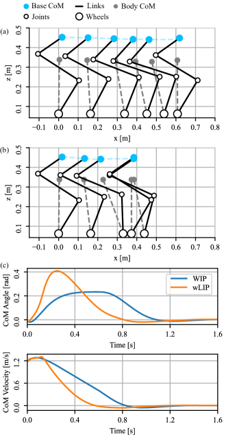
Figure 6: Simulated trajectory of robots controlled WIP and wLIP model. (a) Result of WIP-based LQR. (b) Result of the wLIP-based weight QP controller. (c) Trajectories of the CoM tilting angle and the CoM velocity about the two simulation results. The dashed grey lines represent the virtual link between the CoM and the wheels, and the blue dashed lines denote the trajectories of base CoM.

Remark 3 (Defects of WIP model).

Besides the WIP-based LQR controller tested in this example, we note that there are other controllers, e.g., WBC and MPC [6, 14], that are integrated with WIP model. While changing controllers and parameters might influence the performance in the tested balancing task, it is common to all WIP-based controllers that, the WIP always assumes a rotated base, leading to excessive CAM. Moreover, if used, the linearization of WIP around zero $\vartheta$ is highly inaccurate which causes poor prediction in LQR and MPC. In contrast, as discussed in Remark 1, the wLIP model overcomes these defects during balancing. We believe it is also promising to integrate the wLIP model with other types of controllers to achieve better dynamic performance.

V-C Squatting of WBR

As is mentioned in Section II-B, inspired by human bio-mechanics, we aim to balance the torque distribution in hip and knee joints during squatting task. As our robot is designed to have the same type of motors at the hips and knees, we expect to maintain their torques roughly at the same level to maximize the torque efficiency, i.e., the torque ratio $r_{\tau}$ is approximately 1. Implementing this task requires the incorporation of inertia-aware inverse kinematics (IK) that ensures the moment arms satisfy a specific ratio.

Valid squatting height

Due to the constraints in mechanical design, the WBR has limited squatting height range to ensure unified torque ratio $r_{\tau}$. We first verify the such squatting height range with balanced torque using numerical simulation. With the notation from Fig. 3b, the squatting task transformed to tracking desired CoM height $z^{d}$ could be formulated as

$$\boldsymbol{\Theta}^{*}= \underset{\boldsymbol{\Theta}}{\operatornamewithlimits{argmin}}\;\;(r_{\tau}-1)^{2},$$ (36a)

s.t. $$z=z^{d},\;\delta x=0,$$ (36b)

$$\mathbf{J}_{w}^{\top}\begin{bmatrix}0&m_{c}g\end{bmatrix}^{\top}=\begin{bmatrix}0&\tau_{h}&\tau_{k}\end{bmatrix}^{\top},$$ (36c)

$$\boldsymbol{\Theta}\in[\boldsymbol{\Theta}_{\text{lb}},\boldsymbol{\Theta}_{\text{ub}}],$$ (36d)

where $\boldsymbol{\Theta}=[\theta_{P},\theta_{H},\theta_{K}]$, $\theta_{P}$, $\theta_{H}$, and $\theta_{K}$ are respectively base pitch, hip and knee angles marked in Fig. 3b; $\mathbf{J}_{w}\in\mathbb{R}^{2\times 3}$ is the Jacobian that projects $\dot{\boldsymbol{\Theta}}$ to the planar Cartesian space velocity of the wheel w.r.t the base, $g$ is the gravitational acceleration, $\boldsymbol{\Theta}_{\text{lb}},\boldsymbol{\Theta}_{\text{ub}}$ are the joint position bounds. The equality constraints in (36b) tracks the CoM height command $z^{d}$ and keeps the WBR in static balance, (36c) ensures the validity of inertia aware IK, and (36d) imposes design constraints to the base angles $\boldsymbol{\Theta}$. With the designed planar link inertia information, the optimization problem is solved by IPOPT [42] for a range of $z^{d}$ and fitted by piece-wise polynomials. When performing squatting, the robot tracks only the optimized $\theta_{P}^{*}$ with IK while the other two joint angles will approximate the optimized $\theta_{H}^{*}$ and $\theta_{K}^{*}$, assuming the kinematic model is accurate enough. The optimized results are shown in Fig. 7.

The WBR is commanded to track a linearly increased CoM height trajectory between $z^{d}\in[0.2,0.4]$m. Due to the limitation of mechanical structure like link length, the optimized result provides a unity torque ratio for $z^{d}\in[0.24,0.38]$m, as shown in Fig. 7b. Considering the imperfect tracking which may lead to singular configuration if $z^{d}$ is too high, the $z^{d}$ in the squatting task will be set within $[0.25,0.35]$m for the simulation and experiments.

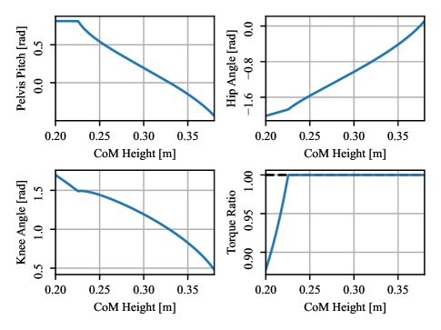
Figure 7: Demonstration of the IPOPT-optimized hip-knee torque ratio during squat. The optimized reference trajectory (a) $\theta_{P}^{*}$, (b) $\theta_{H}^{*}$, and (c) $\theta_{K}^{*}$. (d) The optimized torque ratio $r_{\tau}$. The dashed line denotes the desired ratio 1.

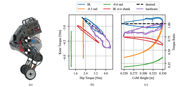
Figure 8: Squat experiment. (a)Squat motion illustration. (b) Hip and knee torque relation. (c) Torque ratio $r_{\tau}$ during squatting. The green and yellow lines denote constant $\theta_{P}$ tracking control at $-0.6$, $-0.3$rad respectively. The blue line denotes the proposed control strategy (36) and the red line denotes (36) without shank inertia. The purple line denotes the hardware experiment result. The black dashed line denotes the desired curve where $r_{\tau}=1$.

Comparison with alternatives

After identifying the valid squatting height range in Section V-C, we control the proposed WBR with the weighted QP controller (33) and compare with other alternatives in simulation. It is common in previous works where the joint angles $\boldsymbol{\Theta}$ are defined to track constant values as previously in [10, 7], we select $\theta_{P}=-0.3$, $-0.6$rad for instances, and simulate the torque ratio during the whole squatting process. Moreover, it is mentioned above that in (36), we need to incorporate precise inertia information with IK (36c) such that the moment arms satisfy the correct ratio. To verify such point, we neglect the shank inertia to form an inaccurate IK and compute the resulting torque ratio during squatting. For all examples, the WBR is commanded to track the desired CoM height $z^{d}(t)=0.3+0.05\sin(t)\in[0.25,0.35]$m, ensuring the CoM height is within the specific range computed above. The simulation results are shown in Fig. 8, the knee and hip torque relation is shown in Fig. 8a while the torque ratio $r_{\tau}$ is shown in Fig. 8b.

We first note that the constant pitch angle tracking strategies, $-0.3$rad (yellow line) and $-0.6$rad (green line) show poor performance in balancing torque distribution: the hip torque is nearly constant in Fig. 8a as the hip moment arm is always the same, the torque ratios are also smaller than 1, showing that the knee motor outputs larger torque than the hip. Tracking trajectory planned by (36) with imprecise model, neglecting shank inertia (red line) shows improved performance than constant pitch angle as (36) provides balance between hip and knee torque, but the imprecise inertia model leads to a steady error to the desired torque ratio, i.e., an approximately $1.2$Nm knee torque shift away from the desired unitary torque ratio (black dashed line). In contrast, the proposed strategy (blue line) could leads to a steady and periodic oscillation around the ideal ratio, indicating that IK formulation with whole-body inertia (36) can provide accurate kinematics reference and that the design can achieve human-like, balanced torque distribution.

Experimental validation

To further demonstrate the validity of our design and control strategy, the designed WBR robot is commanded to perform periodic squatting by track the same CoM height trajectory as in simulation. The experimental results are summarized in Fig. 8 as purple line. We note that due to the inevitable model error, there exists inertia mismatch between the hardware system and the theoretically derived model, leading to error between experimental and theoretical results. Despite such error, the experiment results shows improved performance compared to all other alternatives: it is closer to the desired torque ratio (black dashed line), showing the effectiveness of the control strategy (36) in improving joint torque distribution. The experiment is also presented in the attached video for reference.

V-D Dynamic Performance Test

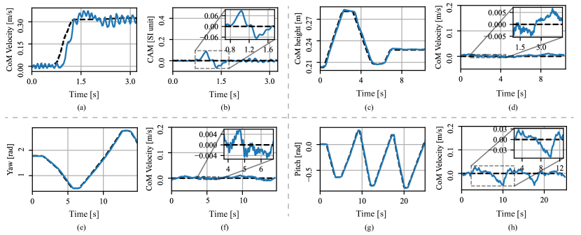
Figure 9: Dynamic performance test. (a-b) The CoM velocity and CAM data in tracking $\dot{x}^{d}_{c}$ command. (c-d) The CoM height and velocity data in tracking $z^{d}$ command. (e-f) The yaw and CoM velocity data in tracking $\phi^{d}$ command. (g-h) The pitch and CoM velocity data in tracking $\psi^{d}$ command. The dashed lines are user references bounded by lower/upper constraints.

In this section, we aim to demonstrate the dynamic performance of the proposed tracking controller (33). As we have five tracking references CoM velocity $\dot{x}_{c}^{d}$, CoM height $z^{d}$, base orientation yaw $\phi\in\mathbb{R}$, pitch $\theta\in\mathbb{R}$, roll $\psi\in\mathbb{R}$, we select the first four to test the dynamics performance, the experiment is performed by selecting one parameter to track random user commands from a remote controller, while the other parameters are commanded to be static. Due to the limitation of mechanical structure, active tracking of roll $\theta$ cannot be implemented, we will test the passive tracking, i.e., balancing, of roll angle in next section. The experiment results of testing dynamic tracking performance are shown in Fig. 9 and recorded in the attached video material for intuitive demonstration.

We note that it is clearly shown that the controller can effectively control the robot to track CoM velocity $\dot{x}^{d}_{c}$ in Fig. 9a while keep the other reference parameters balanced, we show CAM in Fig. 9b for instance. The fluctuation of CAM is zoomed in Fig. 9b, that the maximum fluctuation is only 0.06. We note that the CoM velocity exhibits oscillation in steady states, this is due to the ripple torque of the wheel motors that requires low-level position-based compensation in the motor drivers [43], currently such function is inaccessible to the authors; besides, the minor fluctuation in the balance of other parameters is also inevitable due to the model error. Furthermore, perfect tracking of CoM height $z^{d}$ in Fig. 9c is observed while good balancing performance of other parameters, e.g., $\dot{x}_{c}$ shown in Fig. 9d, is also recorded to show the performance of controller (33). Similarly, the tracking of base orientation, i.e., tracking yaw $\phi$ in Fig. 9e-f and pitch $\theta$ in Fig. 9g-h, also demonstrates good control performance: during the whole motion, the maximum deviation of $\dot{x}_{c}$ is always below $0.03$m/s, i.e., the other parameters are always balanced.

V-E Robustness against External Disturbance

Besides the squatting and tracking performance tested in Section V-C-V-D, it is also important that the WBR system could be robust against unexpected disturbance. In this section, we mainly test the robustness against perturbation from external environment and mobile stability in unknown terrain.

Random external disturbance

To test the robustness of controller (33) against external disturbance, we command the robot to operate static balancing task, and then 1) impose manual shaking on the lateral side of the robot to test if the WBR could maintain stability of roll angle $\psi$ and resume original configuration, 2) kick on the robot to test if the robot could maintain stability after the impact and resume the original configuration and position. The experiment results are shown in Fig. 10 and recorded in the attached video for demonstration.

During the lateral shaking shown in Fig. 10a, we note that the shaking is imposed for around $3.5$s and the roll angle $\theta$ is perturbed around $10^{\circ}$. After perturbation, the controller resumes balance with less than $0.8$s and the WBR is always balanced during the whole procedure. Similarly, in the kicking impact test in Fig. 10b, the WBR is kicked downwards and moves forward around $0.32$m to dissipate the disturbance, the controller spends around $1$s to stabilize and then slowly spend $3$s to return the original position. It is clearly demonstrated that the controller (33) could efficiently and robustly balance the system against external disturbance.

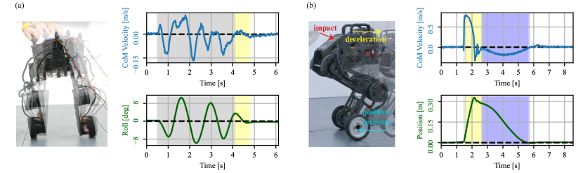
Figure 10: Robustness against unknown external disturbance. (a) Lateral shaking and the recorded data of balancing in CoM velocity $\dot{x}_{c}$ and roll angle $\theta$. (b) Kick impact and the recorded data of balancing CoM velocity $\dot{x}_{c}$ and resuming of position. The dashed black lines denote desired states. The gray area marks the moment when external disturbance is imposed, the yellow area marks the balancing process while the cyan span marks the resuming process to original position.

Unknown terrain in mobility

To test the compliance and robustness against environmental disturbance, i.e., unknown terrain, during locomotion, we command the WBR system to pass a pair of highly inclined symmetric slopes while maintaining the configuration of the WBR. During the process, the CoM velocity $\dot{x}_{c}^{d}$ and yaw $\phi^{d}$ are manually commanded, the other tracking parameters, i.e., $\theta^{d}$, $\psi^{d}$, $z^{d}$ are maintained to constant values (black dashed lines in Fig. 11). The experiment procedure is demonstrated in Fig. 11a and the measured data is shown in Fig. 11b-g, with recorded clip included in the attached video material.

We first note that the CoM velocity is commanded around $0.5$m/s (Fig. 11b), and the yaw is pushed to overcome the disturbances from the ground reaction force (Fig. 11c). Tracking of other parameters are will maintained, the error is small the could be resumed to balance quickly after passing the slopes, as are shown in Fig. 11e-f. Furthermore, we observed that when climbing over the slope, the base height (Fig. 11g) is actively lowered such that the CoM height (Fig. 11f) could be regulated constant, revealing the effectiveness of the proposed controller (33).

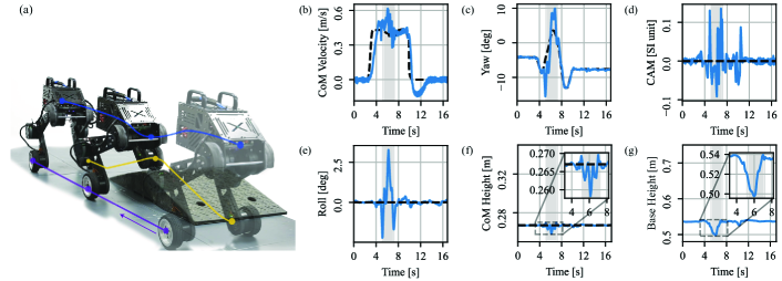
Figure 11: Robustness against unknown terrain. (a) The demonstration of the experiment, the WBR is commanded to pass a pair of highly inclined, symmetrically placed slopes. Trajectories of the base height, left wheel and right wheel are marked with blue, cyan and yellow lines. (b-g) The measured data of CoM velocity $\dot{x}_{c}$, CAM, roll $\psi$, base height, CoM height $z$ and yaw $\phi$ when passing the slopes, process of pass the slopes is marked with gray span in each figure, the black dashed lines denote the tracking commands. To make the control of roll angle compliant to unknown terrain, we reduce the control gains of roll angle $\psi$ to $K_{p}=50$, $K_{d}=5$.

Remark 4 (Computational efficiency).

As the error system (18) and CLF condition (20) are parameterized by $z$, the parameter $\mathbf{P}_{z}$ in (26) is updated in real-time. In the hardware experiment, we adopt the algorithm proposed in [44] to solve the CARE, and the measured average time spent to compute the $\mathbf{P}_{z}\in\mathbb{R}^{6\times 6}$ is within $25$$\mu$s, which is efficient for real-time control.

Numerically, the weighted QP defined in (33) is implemented using the CasADi conic interface [45] to OSQP [46]. The average time spent to solve the weighted QP using OSQP is measured around $200\mu$s. We note that because the control frequency in hardware experiment is at $500$Hz and then the corresponding sampling time $T_{s}$ is $2$ms, computation of (33) is only $10$% of $T_{s}$. Consequently, computation of (33) is efficient for real-time control of the proposed WBR system.

VI Conclusion

In this paper, a serial-legged wheeled bipedal robot is designed based on bio-mechanic analysis of human squatting, aiming to balance the torque distribution between hip and knee motors without losing the large base workspace. It is controlled using a CLF-based weighted QP controller with wLIP model. As a better approximation of wheeled bipedal locomotion by considering variable leg length and wheel torque, the proposed wLIP model is demonstrated to have superior dynamic performance than WIP. The CLF condition provides theoretically guaranteed stability in the presence of various constraints and task-space objectives. In hardware experiments, the deep squatting experiment illustrated that the bionically-designed WBR can realize human-like torque ratio, and the system could perform various tasks including CoM and base state manipulation, and is robust against external disturbances like manual perturbation and irregular terrain.

Current work lacks active adaptability to terrain, leading to lagged adaption and imperfect performance. It is expected to be improved with the help of lidar sensors and cameras. In the future, the wLIP model can be extended for 3D wheeled bipedal dynamic walking in the real world. On the other side, the bio-inspired mechanical design allows further extensions such as adding a robotic arm. With additional DoFs in the sagittal plane to contribute to the CAM, we believe the proposed WBR system could finish more challenging tasks.

References

- [1] V. Klemm et al., “Ascento: A two-wheeled jumping robot,” in Proc. IEEE Int. Conf. Robot. Automat. (ICRA), 2019, pp. 7515–7521.
- [2] S. Wang et al., “Balance Control of a Novel Wheel-legged Robot: Design and Experiments,” in Proc. IEEE Int. Conf. Robot. Automat. (ICRA), 2021, pp. 6782–6788.
- [3] F. Pierrot, C. Reynaud, and A. Fournier, “Delta: a simple and efficient parallel robot,” Robotica, vol. 8, no. 2, p. 105–109, 1990.
- [4] Y.-J. Kim, “Anthropomorphic low-inertia high-stiffness manipulator for high-speed safe interaction,” IEEE Trans. Robot., vol. 33, no. 6, pp. 1358–1374, 2017.
- [5] H. Chen, B. Wang, Z. Hong, C. Shen, P. M. Wensing, and W. Zhang, “Underactuated motion planning and control for jumping with wheeled-bipedal robots,” IEEE Robot. Automat. Lett. (RA-L), vol. 6, pp. 747–754, 2020.
- [6] F. Raza and M. Hayashibe, “Towards robust wheel-legged biped robot system: Combining feedforward and feedback control,” in 2021 IEEE/SICE Int. Sympo. Syst. Integr. (SII), 2021, pp. 606–612.
- [7] J. Yu, Z. Zhu, J. Lu, S. Yin, and Y. Zhang, “Modeling and mpc-based pose tracking for wheeled bipedal robot,” IEEE Robot. and Automat. Lett. (RA-L), vol. 8, no. 12, pp. 7881–7888, 2023.
- [8] Y. Zhuang, Y. Xu, B. Huang, M. Chao, G. Shi, X. Yang, K. Zhang, and C. Fu, “Height control and optimal torque planning for jumping with wheeled-bipedal robots,” in Proc. IEEE Int. Conf. Adv. Robot. and Mechatron. (ICARM), 2021, pp. 477–482.
- [9] Z. Cui, Y. Xin, S. Liu, X. Rong, and Y. Li, “Modeling and control of a wheeled biped robot,” Micromachines, vol. 13, no. 5, 2022.
- [10] T. Liu, C. Zhang, S. Song, and M. Q.-H. Meng, “Dynamic height balance control for bipedal wheeled robot based on ros-gazebo,” in Proc. IEEE Int. Conf. on Robot. and Biomim. (ROBIO), 2019, pp. 1875–1880.
- [11] B. Katz, J. Di Carlo, and S. Kim, “Mini cheetah: A platform for pushing the limits of dynamic quadruped control,” in Proc. IEEE Int. Conf. Robot. Automat. (ICRA). IEEE, 2019, pp. 6295–6301.
- [12] Y.-S. Ha and S. Yuta, “Trajectory tracking control for navigation of the inverse pendulum type self-contained mobile robot,” Robot. Auton. Syst., vol. 17, no. 1, pp. 65–80, 1996.
- [13] V. Klemm et al., “LQR-Assisted Whole-Body Control of a Wheeled Bipedal Robot With Kinematic Loops,” IEEE Robot. Automat. Lett. (RA-L), vol. 5, pp. 3745–3752, 2020.
- [14] H. Cao, B. Lu, H. Liu, R. Liu, and X. Guo, “Modeling and mpc-based balance control for a wheeled bipedal robot,” in Proc. Chin. Control Conf. (CCC), 2022, pp. 420–425.
- [15] S. Xin and S. Vijayakumar, “Online dynamic motion planning and control for wheeled biped robots,” in Proc. IEEE/RSJ Int. Conf. Intell. Robots Syst. (IROS), 2020, pp. 3892–3899.
- [16] W. Zhu, F. Raza, and M. Hayashibe, “Reinforcement learning based hierarchical control for path tracking of a wheeled bipedal robot with sim-to-real framework,” in Proc IEEE/SICE Int. Sympo. Sys Integr (SII), 2022, pp. 40–46.
- [17] J. Zhang, B. Lu, Z. Liu, Y. Xie, W. Chen, and W. Jiang, “A balance control method for wheeled bipedal robot based on reinforcement learning,” in Proc. Chin. Control Conf. (CCC), 2023, pp. 2288–2293.
- [18] J. Zhang, S. Wang, H. Wang, J. Lai, Z. Bing, Y. Jiang, Y. Zheng, and Z. Zhang, “An adaptive approach to whole-body balance control of wheel-bipedal robot ollie,” in Proc. IEEE/RSJ Int. Conf. Intell. Robots Syst. (IROS), 2022, pp. 12 835–12 842.
- [19] B. Recht, “A tour of reinforcement learning: The view from continuous control,” Annu. Rev. Control, Robot., Auton. Syst., vol. 2, pp. 253–279, 2019.
- [20] X. Li, H. Zhou, H. Feng, S. Zhang, and Y. Fu, “Design and experiments of a novel hydraulic wheel-legged robot (wlr),” in Proc. IEEE/RSJ Int. Conf. Intell. Robots Syst. (IROS), 2018, pp. 3292–3297.
- [21] X. Xiong and A. Ames, “3-D Underactuated Bipedal Walking via H-LIP Based Gait Synthesis and Stepping Stabilization,” IEEE Trans. Robot. (T-RO), vol. 38, pp. 2405–2425, 2021.
- [22] J. Reher, C. K. Kann, and A. Ames, “An inverse dynamics approach to control lyapunov functions,” 2020 American Control Conference (ACC), pp. 2444–2451, 2019.
- [23] M. Chadwick, H. Kolvenbach, F. Dubois, H. F. Lau, and M. Hutter, “Vitruvio: An open-source leg design optimization toolbox for walking robots,” IEEE Robot. and Automat. Lett. (RA-L), vol. 5, no. 4, pp. 6318–6325, 2020.
- [24] A. B. Ghansah, J. Kim, M. Tucker, and A. D. Ames, “Humanoid robot co-design: Coupling hardware design with gait generation via hybrid zero dynamics,” in IEEE Conf. Decis. Control (CDC). IEEE, 2023.
- [25] J. Gené-Morales, J. Flandez, A. Juesas, P. Gargallo, I. Miñana, and J. C. Colado, “A systematic review on the muscular activation on the lower limbs with five different variations of the squat exercise,” Journal of Human Sport and Exercise, pp. S1277–S1299, 2020.
- [26] D. Pérez et al., “Relationship of limb lengths and body composition to lifting in weightlifting,” Int. J. Environ. Res. Public Health, vol. 18, pp. 1–16, 01 2021.
- [27] J. D. Wong, M. F. Bobbert, A. J. van Soest, P. L. Gribble, and D. A. Kistemaker, “Optimizing the distribution of leg muscles for vertical jumping,” PLOS ONE, vol. 11, no. 2, p. e0150019, Feb 2016.
- [28] A. J. Van Soest, A. L. Schwab, M. F. Bobbert, and G. J. van Ingen Schenau, “The influence of the biarticularity of the gastrocnemius muscle on vertical-jumping achievement,” J. Biomech., vol. 26, no. 1, p. 1–8, Jan 1993.
- [29] Y. Chen, Z. Xie, K. Huang, H. Lin, and J. Chang, “Biomechanical Analysis to Determine the Most Effective Posture During Squats and Shallow Squats While Lifting Weights in Women,” J. Med. Biol. Eng., vol. 40, pp. 334–339, 2020.
- [30] R. Featherstone, Rigid body dynamics algorithms. Springer, 2014.
- [31] J. Carpentier, G. Saurel, G. Buondonno, J. Mirabel, F. Lamiraux, O. Stasse, and N. Mansard, “The Pinocchio C++ library : A fast and flexible implementation of rigid body dynamics algorithms and their analytical derivatives,” in Proc. IEEE/SICE Int. Sympo. Syst. Integr. (SII), 2019, pp. 614–619.
- [32] S. Kajita, F. Kanehiro, K. Kaneko, K. Yokoi, and H. Hirukawa, “The 3d linear inverted pendulum mode: a simple modeling for a biped walking pattern generation,” in Proc. IEEE/RSJ Int. Conf. Intell. Robots Syst., vol. 1, 2001, pp. 239–246 vol.1.
- [33] Y. Gong and J. Grizzle, “Angular momentum about the contact point for control of bipedal locomotion: Validation in a lip-based controller,” arXiv preprint abs/2008.10763, 2021.
- [34] P. M. Wensing and D. E. Orin, “High-speed humanoid running through control with a 3d-slip model,” in Proc. IEEE/RSJ Int. Conf. Intell. Robots Syst. (IROS), 2013, pp. 5134–5140.
- [35] A. D. Ames, S. Coogan, M. Egerstedt, G. Notomista, K. Sreenath, and P. Tabuada, “Control barrier functions: Theory and applications,” in 2019 18th European Control Conference (ECC), 2019, pp. 3420–3431.
- [36] R. Grandia et al., “Nonlinear model predictive control of robotic systems with control lyapunov functions,” in Robotics: Science and Systems, 2020.
- [37] D. Kim, J. D. Carlo, B. Katz, G. Bledt, and S. Kim, “Highly Dynamic Quadruped Locomotion via Whole-Body Impulse Control and Model Predictive Control,” arXiv preprint abs/1909.06586, 2019.
- [38] Y. Ding, C. Khazoom, M. Chignoli, and S. Kim, “Orientation-aware model predictive control with footstep adaptation for dynamic humanoid walking,” in Proc. IEEE-RAS Int. Conf. Humanoid Robots (Humanoids), 2022, pp. 299–305.
- [39] J. Shen, J. Zhang, Y. Liu, and D. Hong, “Implementation of a robust dynamic walking controller on a miniature bipedal robot with proprioceptive actuation,” in Proc. IEEE-RAS Int. Conf. Humanoid Robots (Humanoids), 2022, pp. 39–46.
- [40] C. Dario Bellicoso, C. Gehring, J. Hwangbo, P. Fankhauser, and M. Hutter, “Perception-less terrain adaptation through whole body control and hierarchical optimization,” in Proc. IEEE-RAS Int. Conf. on Humanoid Robots (Humanoids), 2016, pp. 558–564.
- [41] J. Hwangbo, J. Lee, and M. Hutter, “Per-contact iteration method for solving contact dynamics,” IEEE Robot. Automat. Lett. (RA-L), vol. 3, no. 2, pp. 895–902, 2018.
- [42] A. Wächter and L. T. Biegler, “On the implementation of an interior-point filter line-search algorithm for large-scale nonlinear programming,” Math. Program., vol. 106, pp. 25–57, 2006.
- [43] M. Piccoli and M. Yim, “Anticogging: Torque ripple suppression, modeling, and parameter selection,” Int. J. Robot. Res. (IJRR), vol. 35, no. 1-3, pp. 148–160, 2016.
- [44] A. Laub, “A schur method for solving algebraic riccati equations,” IEEE Trans. Autom. Control, vol. 24, no. 6, pp. 913–921, 1979.
- [45] J. A. E. Andersson, J. Gillis, G. Horn, J. B. Rawlings, and M. Diehl, “CasADi: a software framework for nonlinear optimization and optimal control,” Math. Program. Comput., vol. 11, pp. 1–36, 2018.
- [46] B. Stellato, G. Banjac, P. Goulart, A. Bemporad, and S. Boyd, “OSQP: an operator splitting solver for quadratic programs,” Math. Program. Comput., pp. 1–36, 2017.