Deep Active Audio Feature Learning in Resource-Constrained Environments

Abstract

The scarcity of labelled data makes training DNN models in bioacoustic applications challenging. In typical bioacoustics applications, manually labelling the required amount of data can be prohibitively expensive. To effectively identify both new and current classes, DNN models must continue to learn new features from a modest amount of fresh data. Active Learning (AL) is an approach that can help with this learning while requiring little labelling effort. Nevertheless, the use of fixed feature extraction approaches limits feature quality, resulting in underutilization of the benefits of AL. We describe an AL framework that addresses this issue by incorporating feature extraction into the AL loop and refining the feature extractor after each round of manual annotation. In addition, we use raw audio processing rather than spectrograms, which is a novel approach. Experiments reveal that the proposed AL framework requires 14.3%, 66.7%, and 47.4% less labelling effort on benchmark audio datasets ESC-50, UrbanSound8k, and InsectWingBeat, respectively, for a large DNN model and similar savings on a microcontroller-based counterpart. Furthermore, we showcase the practical relevance of our study by incorporating data from conservation biology projects.

1 Introduction

DNN models require a large amount of labelled data and long training times to extract high-quality hierarchical features [1], limiting their success to domains with abundant labelled data [2]. Our research focuses on bioacoustic applications in conservation biology. In this domain, generating labelled training samples usually requires the manual extraction of short segments (e.g. individual bird calls) from continuous recordings that cover days, weeks, or even longer periods. The relevant segments often occur only relatively infrequently in these recordings. Acquiring sufficient amounts of high-quality labelled data at the start of a project is thus often impractical. Ideally, we would like to bootstrap the process of sample collection with a small number of labelled samples. A first (tentative) classifier trained on these can then be used to suggest further relevant samples which are screened by an expert and subsequently used to train an improved classifier. The process is then repeated until the required performance is reached. Indeed, this is often done in real-world applications in an ad-hoc fashion. A more principled approach to keep the labelling effort acceptable using an incremental strategy is to employ Active Learning (AL), a semi-supervised machine learning technique [3].

As an iterative learning method, AL is intended to speed up learning, especially when a large labelled dataset is unavailable for traditional supervised learning [4, 1, 2]. AL algorithms combine intelligent acquisition functions to select samples that promise the best differential learning [2] with specialized incremental training techniques [3, 2].

Here, we investigate the suitability of AL for bioacoustic classification. From a high-level perspective, bioacoustic classification usually proceeds in two steps: the first step extracts a vector of characteristic features from the audio, while the second step performs a classification based on this feature vector. While Active Learning has been used in (bio)acoustic applications before (see Section 2), previous works have only attempted to improve the classification phase based on fixed feature extraction methods [2, 5, 6, 7, 3, 8, 9, 10, 11, 12, 13, 14, 13, 15, 16, 1]. As a result, the primary advantage of the Deep Active Learning (DAL) method is never fully realized.

We hypothesize that retraining the feature extraction method itself in the iterative training loop will improve the performance of active learning and allow us to further reduce the number of training samples required. Our experiments demonstrate the validity of this hypothesis using three standard benchmarks: ESC with 50 classes (ESC-50) [17], UrbanSound8k (US8K) [18], and InsectWingBeat (iWingBeat) [19]. Including the feature extraction in the active learning loop results in a model that requires significantly less labelling effort than existing DAL methods. For the three datasets, our approach reduces the labelling effort required by 14.28%, 66.67%, and 50%, respectively.

We demonstrate the method’s practical relevance beyond standard benchmarks by applying it to data from a real-world conservation project.

In previous work [20], we have shown that bioacoustic classification can be achieved by surprisingly small models that allow us to perform the recognition in-situ in field recording units. We show that our proposed active learning approach functions independently of the network size and that its advantages carry over to such tiny networks.

2 Current Literature

The fundamental issue our work is addressing is that, traditionally, in the AL process, the feature extraction process is static instead of being included in the incremental active learning loop.

2.1 Audio Feature Extraction Approaches

A significant variety of different audio feature extraction strategies are in use. Arguably, the most widely used methods are based on spectrograms (e.g., Mel Frequency Cepstral Coefficients (MFCC) [8] including its first and second-order derivatives [11], Log Power Mel Spectrogram (LPMS) [5], Chromagram [5], statistics of MFCCs in each audio segment [11], etc.).

An alternative is the use of raw audio Time Series (TS) as input to a CNN and to let the feature extractor be learned as part of the model [20, 21, 22, 23, 24].

Pre-trained DNN models such as VGGish [25] are also in use, as well as a mixture of hand-crafted features along with automatic features from the time-frequency domain of the audio signal used in [16] and learned dictionary-based techniques such as Gabor Dictionary [26].

2.2 Overview of Deep Active Learning

The basic idea behind active learning is that if a Machine Learning (ML) algorithm is allowed to choose which data to learn from, it may be able to improve its accuracy while using fewer training labels [4, 1]. Typically, AL algorithms request human annotators to label the data instances for learning.

The essential components of an AL technique are the selection of samples for human annotation, incremental training of a classifier with the annotated data, and labelling the remaining samples with the trained classifier [4, 1, 2, 3]. This is an iterative process. The quantity of samples that can be manually annotated is usually assumed as a fixed labelling budget.

As it is difficult to train a Deep Learning (DL) model to achieve acceptable performance with small amounts of data, the majority of works from the literature (e.g., [27, 8, 5, 6, 10, 13]) employ ML algorithms such as Random Forest (RF) [28], Support Vector Machine (SVM) [29], K-Nearest Neighbors (K-NN) Classifier [30], and Logistic Regression (LR) [31].

There are a variety of sample selection techniques or acquisition functions available. Random sample selection, uncertainty sampling [32] (e.g., least confidence, margin of confidence, etc.), diversity sampling (e.g., medoid-based AL [8], furthest traversal [33], cluster-based outliers, model-based outliers, etc.), query-by-committee [34] and expected error reduction [7] are commonly used examples of such sample selection techniques. However, as our acquisition function, we employ the BADGE [2] sample selection technique, which takes predicted uncertainty and sample variety into account to pick the most problematic samples. This is the only approach that delivers satisfactory results on the datasets used in this study. The availability of the implementation code in a public repository further ensures the reproducibility of this method.

2.3 Related Works

The majority of contemporary literature has been devoted to event classification. Han et al. [3] employ the open-source openSMILE [27] toolkit to extract audio features from the FindSound [35] dataset, the least confidence sampling strategy for sample selection, and SVM with linear kernels to train and classify the audio events. The same feature extraction toolkit and classifier are utilized by Qian et al. [9] in the AL system for the classification of bird sounds. They select samples using a random selection technique for human annotation and continue annotating until the budget runs out or the performance of the classifier is not adequate.

Shuyang et al. [8] employ MFCC and its first and second-order derivatives to extract features from audio data. They further use the statistics of MFCCs in each segment: minimum, maximum, median, mean, variance, skewness, kurtosis, median, and variance of the first and second-order derivatives in [11]. They cluster the data using k-medoid clustering and annotate the medoids of each cluster as local representatives. The label is then propagated throughout the cluster. Once the budget for annotation is exhausted, an SVM and an RF are trained to predict the labels in the former and the latter work, respectively. If there is a discrepancy between propagated and predicted labels, the labels are submitted to humans for correction.

Coleman et al. [5] use MFCC, LPMS, and Chromagram for audio feature extraction from the ESC-50 [36] dataset, train SVM with a small amount of annotated data for prediction of the labels of other samples, and use the smallest confidence scores to select samples for further human annotation. Hilasaca et al. [6] also extract features from spectrograms for soundscape ecology data, cluster the data using k-medoid clustering, and select samples from clusters using random, medoid (samples closest to the cluster centroid), contour (samples furthest from the centroid), and their combinations, for human annotation. They use the RF classifier to predict the labels for the rest of the data.

Kholghi et al. [10] use acoustic indices for feature extraction, k-means clustering, and hierarchical clustering algorithms to cluster the data, and randomly listen to sounds from each cluster for human annotation. They train RF using the annotated data and use it to predict the labels.

Ji et al. [14] and Qin et al. [12] use a Gabor Dictionary [26] and a learned dictionary for their AL based audio classification task on the US8K and ESC-50 datasets. Both use k-medoid clustering to cluster the data and manually label the medoid of each cluster and propagate the labels to the clusters.

Ash et al. [2] and Shi et al. [16] retrain the model in every iteration of human annotation and use the final trained model for labelling at the end of the learning process. Ash et al. [2] adopt diverse gradient embeddings and the k-means++ [37] seeding algorithm in their acquisition function (i.e., BADGE) for taking predictive uncertainty and sample diversity into account; however, the proposed method has only been evaluated on image data. Shi et al. [16], on the other hand, used data with extremely low-frequency of 1kHz and manually engineered the features. They evaluated their approach on ECG recordings obtained from patients with atrial fibrillation. Unlike the previous studies, Wang et al. [13] extracted features from the sonic sensor data using a pre-trained VGGish audio model [25]. They selected samples using an uncertainty sampling technique (i.e., least confidence score) and trained the RF classifier to label the data after human annotation.

In contrast to audio event classification, Kim and Pardo [38, 39] utilize MFCC to extract acoustic features from the DCASE2015 [40] dataset for audio event detection. They calculate the distance among the samples using the nearest neighbour algorithm, rank the samples nearest to the previously annotated sample as high, and choose them for further annotation by a human expert. Shuyang et al. [15] use the spectrogram of TUT Rare Sound Events 2017 [41] and TAU Spatial Sound Events 2019 [42] datasets [15] and change point detection to identify segments from the spectrograms that have events. The segments are clustered using k-medoid clustering, and the medoid of each cluster is annotated. The samples for human annotation are picked using the mismatch-first-farthest traversal approach suggested in their earlier study [11]. In order to detect and classify the rest of the samples, they train a DNN model architecture presented in [43].

According to the above discussion, k-medoid clustering [44] and the Farthest Traversal [33] appear to be the most popular sample selection techniques. However, due to their computational complexity, they do not scale to large amounts of data.

Importantly, all the proposed AL techniques are based on fixed feature sets that do not change throughout the AL life cycle. When a pre-trained model is used to extract features, it is never refined. To the best of our knowledge, it has never been investigated whether the fixed feature set is flexible enough to accommodate the model’s behaviour to time-varying data features. Our work aims to integrate the feature extractor into the active learning loop so that it can be refined with each iteration. To make learned feature extraction as flexible as possible, we start from a raw audio-based automatic feature extraction technique proposed by Mohaimenuzzaman et al. [20, 21] for end-to-end audio event classification.

3 Proposed Active Learning Framework

Figure 1 depicts the detailed construction of the proposed Deep Active Feature Learning (DAFL) approach.

Figure 1: The detailed architecture of the proposed DAFL where the red arrow indicates how the feature extractor is incorporated in the AL loop. Conventional systems use the black path instead of the red path for the active learning loop.

A pre-trained DNN model is employed as a feature extractor. We have used ACDNet [20] as the feature extractor. Figure 2 depicts the ACDNet architecture for an input length of 30,225.

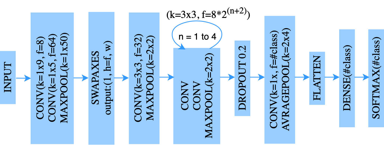
Figure 2: ACDNet architecture for an input length of 30,225, where k and f represent kernel size and number of filters, respectively, and $n\in\{2,\ldots,6\}$.

DAFL allows us to fine-tune the feature extractor. The output layer (i.e. the final dense and softmax layers) is removed from the pre-trained model to accomplish this. We adopt the BADGE [2] sample selection technique in our acquisition function, which combines diverse gradient embeddings and the k-means++ [37] seeding algorithm to take predictive uncertainty and sample diversity into consideration to identify the most difficult samples. The adoption of BADGE is motivated by the fact that alternative sample selection strategies performed poorly for the datasets we used. For instance, the best sample selection technique proposed by Qin et al. [12] has a prediction accuracy of $66\%$ after 2,000 annotations on the US8K dataset, which is not comparable to the results of the BADGE sample selection method (see Table 1).

The feature extractor is fine-tune d in each iteration of human annotation (simulated) on the annotated examples to improve feature embeddings. The previously extracted features are then replaced with new features extracted from the fine-tune d model. This iterative process is repeated until the labelling budget is exhausted or a desirable level of classification accuracy is attained. We then retrain the classifier(s) using the extracted features from the feature extractor. We present our proposed system in Algorithm 1.

Input: DNN Model ($M$), Labeling Budget ($B$), Fine-tune Epochs ($E$), Performance Threshold ($P_{thres}$), No. of Classes ($C$)

Output: Labeled Data ($L$)

Data: Labeled Set ($S_{l}$), Validation set ($S_{v}$), Test Set ($S_{d}$), Unlabeled Pool ($S_{u}$)

1

2$M_{found}\longleftarrow\textit{FALSE\/}$

3 $N\longleftarrow$ no. of samples to be selected

4 $AF\longleftarrow$ Acquisition Function

5 $HA\longleftarrow$ Human Annotation

6 $l_{c}\longleftarrow$ $GetLayerCount(M)$

7

/* last convolution index */

8 $lconv\longleftarrow l_{c}-2$

/* Replace the filters of the last convolution and train */

9 $M\longleftarrow M.layers[lconv].filters\longleftarrow 5*C)$

10 $M\longleftarrow Train(M)$

11

12while $B>len(S_{l})$ and $\textit{NOT\/}\;M_{found}$ do

       /* Keep layers up to the last convolution */

13       $M_{f}\longleftarrow M-M[0:lconv]$

14       $S\longleftarrow AF(M_{f}(N))$

15       $S_{a}\longleftarrow HA(S)$

16       $S_{u}\longleftarrow S_{u}-S_{a}$

17       $S_{l}\longleftarrow S_{l}\cup S_{a}$

18       $S_{t}\longleftarrow S_{a}\cup S_{t}[$Random $len(S_{a})$ samples$]$

19      

20      $val\longleftarrow 0.0$

21       foreach $e$ in $E$ do

22             $M^{\prime}\longleftarrow$ Fine-tune $M$ on $S_{t}$ by minimizing KLD loss

23             $val^{\prime}\longleftarrow M^{\prime}(S_{v})$

24             if $val^{\prime}>val$ then

25                   $val\longleftarrow val^{\prime}$

26                   $M\longleftarrow M^{\prime}$

27            

28      

29      $R_{es}\longleftarrow M(S_{d})$

30       if $R_{es}\geq P_{thres}$ then

31             $M_{found}\longleftarrow\textit{TRUE\/}$

32            

33      

34

35$L\longleftarrow M(S_{u})\cup S_{l}$

36

37return $L$

Algorithm 1 DAFL

4 Comparative Analysis

In this section, we compare the performance of DAFL with the existing DAL techniques and a baseline technique that we refer to as Deep Incremental Learning (DIcL). In DIcL, the samples are chosen at random for annotation. In contrast, the DAL and DAFL experiments use the BADGE [2] sample selection technique, and the model is fine-tune d on the newly annotated samples. The implementation of BADGE is retrieved from Ash [45] and used in our AL implementation. DIcL is thus the same as DAFL but without a targeted sample acquisition method.

This study employs three standard benchmark datasets: ESC-50, US8K and iWingBeat. To determine the fine-tuning strategy, a preliminary study was conducted. Experiments show that fine-tuning the entire model produces the best results (see Section 4.1). We begin by contrasting the performance of DIcL and DAL. For the DAL experiments, we used three different classifiers available in scikit-learn [46]: K-Neighbors Classifier, Logistic Regression, and Ridge Classifier. These methods are referred to as Active Learning with Logistic Regression (AL-LogisticReg), Active Learning with K-Neighbors Classifier (AL-KNC) and Active Learning with Ridge Classifier (AL-RidgeC), respectively. After analyzing the data, we choose the best method for each dataset and compare its performance to that of DAFL on each of the three datasets.

Our analysis shows that for ESC-50 and US8K, AL-RidgeC and AL-LogisticReg outperform DIcL, whereas DIcL outperforms DAL for iWingBeat. We then compared the performance of these approaches to that of our proposed DAFL and discovered that DAFL performed significantly better. DAFL requires approximately 14.3%, 66.67%, and 47.4% less labeling effort (according to Table 1) than other techniques for ESC-50, US8K and iWingBeat datasets, respectively. The same set of experiments is performed with Micro-ACDNet, which is 97.22% smaller than ACDNet and uses 97.28% fewer floating point operations (FLOPs) [20]. DAFL outperforms all other approaches on all three datasets, requiring 42.85%, 66.67%, and 60% less labeling effort, respectively. This supports the hypothesis we set out to investigate: including feature extraction in the AL loop improves performance and reduces labelling effort.

4.1 NoFreeze vs. Freeze Layers for Deep Incremental Learning

Our first experiment is designed to show whether the inclusion of feature extraction in the active learning loop is, in principle, useful. To this end, we use three distinct strategies to fine-tune the pre-trained ACDNet in this preliminary analysis for DIcL, i.e. active learning with random sample acquisition.

• no-freeze: all ACDNet layers have the ability to fine-tune their weight.

• fixed-freeze: only the last three layers are allowed to fine-tune. This is based on the notion that the initial layers perform feature extraction while the last three layers perform classification.

• scheduled-freeze: the last three layers are unfrozen for a few epochs, then two more layers for a few more epochs, and finally two more layers for a few more epochs.

This study was conducted using the ESC-50 [17] dataset. Experiment results show that fine-tuning the entire network yields the best results (see Figure 3).

Figure 3 (results also reported in Table 8) shows that the model’s performance is significantly improved through the fine-tuning process when the no-freeze policy is followed. This already gives clear evidence that it is useful to include fine-tuning the feature extraction layer in the active learning loop. As a result, we will adopt the “no-freeze” strategy as fine-tuning for the remainder of this paper.

Figure 3: Fine-tuning ACDNet in different settings (no-freeze, fixed-freeze and scheduled-freeze) for incremental learning.

4.2 Analysis with Full-sized ACDNet Model

The next experiment is designed to select the best-performing conventional DAL strategy for our problem. The winning method will subsequently be compared with the proposed DAFL.

As in Mohaimenuzzaman et al. [20], we represent accuracy as a 95% Confidence Interval (95%CI) [47] calculated using bootstrap confidence intervals [48, 49]. We used bootstrap sampling with replacement to test the model 1,000 times on the test sets of all the datasets to calculate the 95%CI (see Equation 1 following Mohaimenuzzaman et al. [20]).

$$95\%CI=\mu\pm Z\frac{\sigma}{\sqrt{N}},$$ (1)

where $\mu$ is the average accuracy of all the tests, $Z=1.96$ [47], $\sigma$ is the standard deviation, and $N$ is the total number of tests.

Note that all samples used in this research have been labelled by human experts. We simulate the “human annotation” process by withholding the labels of data at the start of the experiment and placing the data in the unlabeled pool. We then deliver the withheld labels on demand as the acquisition picks these unlabelled samples, just as a human expert would. In the remainder of this paper, we refer to this as “simulated human annotation”. While there is no human direct interaction with the process, this clearly delivers the exact same results.

4.2.1 Deep Incremental Learning (DIcL) vs Existing Deep Active Learning (DAL) with ACDNet

We first pitch DIcL against three conventional DAL strategies: AL-KNC, AL-LogisticReg and AL-RidgeC. We present the analyses on the three datasets in the following order: ESC-50, US8K, and iWingBeat.

Figure 4 (data also reported in Table 9), shows that AL-RidgeC obtains the highest prediction accuracy achieved by DIcL (i.e., $65.43\%$) in only 3 iterations on the ESC-50 dataset, saving $\approx 57\%$ of the labelling budget. At the end of seven simulated human labelling iterations, AL-RidgeC achieves the highest accuracy of $67.94\%$.

Figure 4: DIcL vs DAL that shows that the AL-based approach AL-RidgeC performs better than incremental learning on the ESC-50 dataset.

The same comparative analysis is performed on the US8K dataset. Figure 5 (see data in Table 10) demonstrates that AL-KNC and AL-LogisticReg learn to predict the data significantly better than DIcL. Furthermore, after only 2 iterations, AL-LogisticReg achieves the highest prediction accuracy achieved by DIcL (i.e., $88.19\%$), saving nearly $86.67\%$ of the labelling budget. As US8K contains more data than ESC-50, we perform fifteen iterations of human labelling for DIcL and the DAL process.

Figure 5: DIcL vs DAL that shows that the AL-based approach AL-LogisticReg performs better than incremental learning on the US8K dataset.

Somewhat surprisingly, Figure 6 (data reported in Table 11) reveals that DIcL has the highest prediction accuracy on the iWingBeat dataset. In contrast to the results on the other datasets, the performance of the initial model and the model obtained after human annotations (simulated) and fine-tuning do not differ significantly for this dataset. Since this dataset contains more labelled samples than the previous two, we run twenty human annotation iterations.

Figure 6: DIcL vs DAL on iWingBeat dataset

4.2.2 DAFL vs Others with ACDNet

We now compare the performance of the three best methods for three datasets (AL-RidgeC for ESC-50, AL-LogisticReg for US8K, and DIcL for iWingBeat) from the previous section to that of DAFL. We use the same testing procedures as in the previous sections. In the case of DAFL, we use ACDNet as the learning and classification model rather than DAL. The primary distinction between previous methods and DAFL is that it is calibrated using annotated samples and the feature extractor is updated. We begin by comparing the performances of models derived from various techniques, and then we examine the statistical significance of the performance of the winning model.

The performances of DAFL in terms of the 95% Confidence Interval (95%CI) are summarized, together with the results of the three best approaches (described in Tables 9, 10, and 11) in Table 1. Iteration-wise performance for ESC-50, US8K, and iWingBeat datasets are displayed in the columns labeled 95%CI-ESC-50, 95%CI-US8K, and 95%CI-iWingBeat, respectively.

Learning	95%CI-ESC-50		95%CI-US8K		95%CI-iWingBeat
Loops	AL-RidgeC	DAFL	AL-LogisticReg	DAFL	DIcL	DAFL
0	57.79 $\pm$ 0.16	55.81 $\pm$ 0.16	87.55 $\pm$ 0.05	86.97 $\pm$ 0.06	66.08 $\pm$ 0.04	66.08 $\pm$ 0.04
1	59.54 $\pm$ 0.14	63.76 $\pm$ 0.14	87.48 $\pm$ 0.05	85.93 $\pm$ 0.05	66.94 $\pm$ 0.04	66.59 $\pm$ 0.04
2	62.58 $\pm$ 0.15	64.15 $\pm$ 0.15	88.25 $\pm$ 0.04	86.82 $\pm$ 0.05	66.50 $\pm$ 0.04	66.99 $\pm$ 0.04
3	65.19 $\pm$ 0.14	65.00 $\pm$ 0.16	88.08 $\pm$ 0.04	87.15 $\pm$ 0.06	66.21 $\pm$ 0.04	67.57 $\pm$ 0.04
4	67.00 $\pm$ 0.15	65.94 $\pm$ 0.14	88.00 $\pm$ 0.05	87.09 $\pm$ 0.05	66.63 $\pm$ 0.04	67.13 $\pm$ 0.04
5	67.10 $\pm$ 0.15	67.28 $\pm$ 0.15	87.96 $\pm$ 0.05	88.59 $\pm$ 0.06	67.19 $\pm$ 0.04	67.40 $\pm$ 0.04
6	67.73 $\pm$ 0.15	68.74 $\pm$ 0.14	87.96 $\pm$ 0.05	88.20 $\pm$ 0.05	67.30 $\pm$ 0.04	67.76 $\pm$ 0.04
7	67.94 $\pm$ 0.14	70.02 $\pm$ 0.12	87.79 $\pm$ 0.05	88.94 $\pm$ 0.06	67.79 $\pm$ 0.04	67.66 $\pm$ 0.04
8	-	-	88.08 $\pm$ 0.04	88.62 $\pm$ 0.05	67.11 $\pm$ 0.04	68.10 $\pm$ 0.04
9	-	-	88.16 $\pm$ 0.05	88.60 $\pm$ 0.05	67.32 $\pm$ 0.04	68.03 $\pm$ 0.04
10	-	-	88.25 $\pm$ 0.04	88.70 $\pm$ 0.06	67.20 $\pm$ 0.04	68.86 $\pm$ 0.04
11	-	-	88.18 $\pm$ 0.05	88.75 $\pm$ 0.06	67.97 $\pm$ 0.04	68.95 $\pm$ 0.04
12	-	-	88.21 $\pm$ 0.05	88.80 $\pm$ 0.05	67.07 $\pm$ 0.04	68.90 $\pm$ 0.04
13	-	-	88.48 $\pm$ 0.06	89.01 $\pm$ 0.06	67.27 $\pm$ 0.04	69.05 $\pm$ 0.04
14	-	-	88.17 $\pm$ 0.05	89.20 $\pm$ 0.06	66.66 $\pm$ 0.04	69.29 $\pm$ 0.04
15	-	-	88.31 $\pm$ 0.05	89.45 $\pm$ 0.05	67.54 $\pm$ 0.04	69.32 $\pm$ 0.04
16	-	-	-	-	67.50 $\pm$ 0.04	69.76 $\pm$ 0.04
17	-	-	-	-	67.65 $\pm$ 0.04	70.12 $\pm$ 0.04
18	-	-	-	-	67.62 $\pm$ 0.04	70.04 $\pm$ 0.04
19	-	-	-	-	68.27 $\pm$ 0.04	70.18 $\pm$ 0.04
20	-	-	-	-	68.16 $\pm$ 0.04	70.13 $\pm$ 0.04

Table 1: DIcL vs DAL vs DAFL on All Datasets

Figure 7 is derived from Table 1, columns 95%CI-ESC-50. It compares the performance of AL-RidgeC and DAFL on the ESC-50 dataset. AL-RidgeC achieves the highest accuracy ($69.94\%$) in the seventh iteration, whereas DAFL reaches that accuracy in the sixth iteration ($68.74\%$), saving 14.3% of the labelling budget.

Figure 7: AL-RidgeC vs DAFL on ESC-50. DAFL reaches the maximum performance of AL-RidgeC at an earlier stage of the training.

Figure 8 shows a comparison of the performance of AL-LogisticReg and DAFL on the US8K dataset (results also reported in Table 1, columns 95%CI-US8K). AL-LogisticReg achieves the highest prediction accuracy ($88.48\%$) in the thirteenth iteration, but DAFL achieves that accuracy ($88.59\%$) in just five iterations, saving $66.67\%$ of the labeling budget.

Figure 8: AL-LogisticReg vs DAFL on US8K. DAFL reaches the maximum performance of AL-LogisticReg at an earlier stage of the training.

Figure 9 illustrates a comparison of the performance of DIcL and DAFL on the iWingBeat dataset (the data is also reported in Table 1, columns 95%CI-iWingBeat). DIcL achieves the highest prediction accuracy ($68.86\%$) in the thirteenth iteration, while DAFL achieves that accuracy ($68.86\%$) in only five iterations, saving $47.4\%$ of the labeling budget.

Figure 9: DIcL vs DAFL on iWingBeat.DAFL reaches the maximum performance of AL-LogisticReg at an earlier stage of the training.

From the above comparative study, we observe that DAFL significantly outperforms the best-performing methods of the preceding section, both in terms of final accuracy for a given labelling budget as well as in terms of labelling budget required for a given target performance. On the ESC-50, US8K, and iWingBeat datasets, DAFL requires approximately 14.3%, 66.67%, and 47.4% less labeling effort than its counterparts, respectively.

To validate the above findings, we now assess the statistical significance of DAFL performance. To measure the statistical significance of each model’s performance, we employ the statistical significance test described in [50]. In particular, we use a Friedman test [51] to reject the null hypothesis of no difference within the whole group of methods. Then, in accordance with Benavoli et al. [52], we conduct a pairwise post-hoc analysis using the Wilcoxon signed-rank test [53] and Holm’s correction [54, 55], with an initial significance level of $\alpha=5\%$. As a graphical depiction, we use Demšar [56]’s Critical Difference (CD) diagram. In the CD diagram, a thick horizontal line shows that the differences in the accuracy of a set of classifiers are not statistically significant. The horizontal scale at the top indicates the ranks of the learning methods, and the numbers adjacent to them indicate the calculated score used to determine the rank of each method.

Figure 10 depicts the statistical significance of the final models produced after completing all human annotation iterations on the ESC-50 dataset for DIcL, DAL, and DAFL. According to the figure, all the models perform statistically significantly differently. It demonstrates that the model produced by DAFL outperforms other models, ranking top among them.

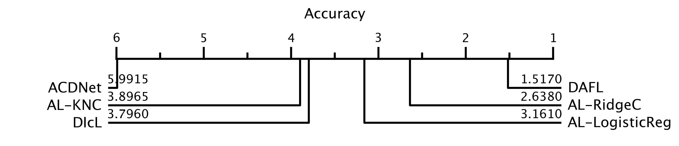
Figure 10: CD diagram showing statistical significance of the learning methods on the ESC-50 dataset.

An analogous statistical analysis is shown in Figure 11 for the US8K dataset. It illustrates that the model produced by DAFL outperforms other models and ranks highest among them.

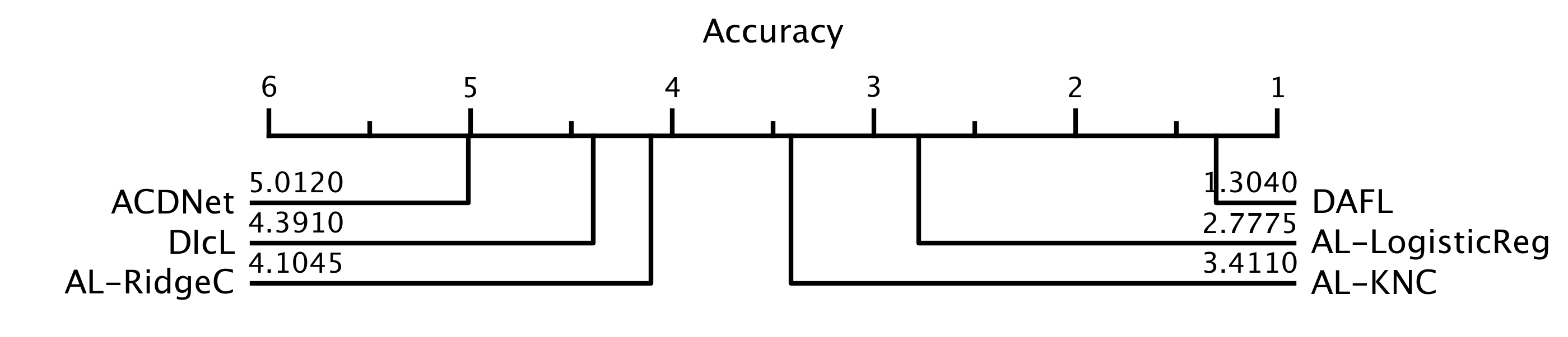
Figure 11: CD diagram showing statistical significance of the learning methods on the US8K dataset.

The situation is the same regarding the iWingBeat dataset. Figure 12 shows that the DAFL-generated model outperforms other models and ranks first among them.

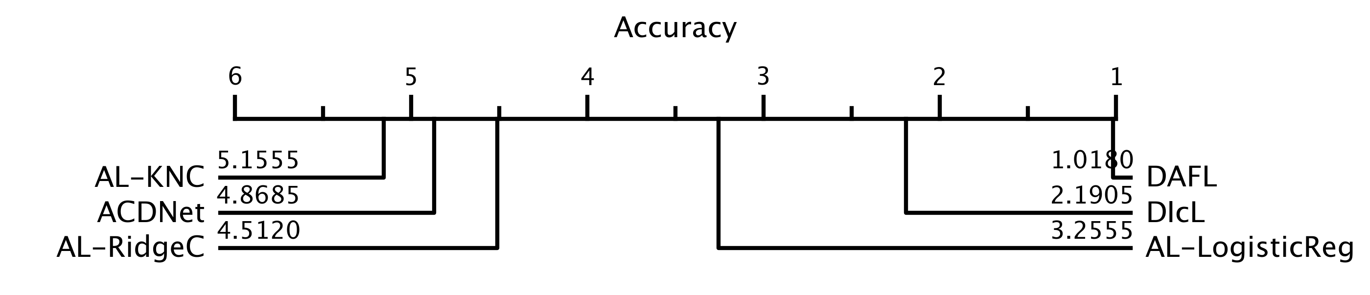
Figure 12: CD diagram showing statistical significance of the learning methods on iWingBeat dataset.

4.3 Analysis with Edge-based Model

In the preceding section, we illustrated the benefit of DAFL for ACDNet, a large architecture designed to run on performant hardware. Now, we repeat the study with Micro-ACDNet [20], an extremely small network operating on Microcontroller Units (MCUs), to investigate if the benefits are retained when moving to very small models. Table 2 summarizes the performances of DAFL in terms of the 95%CI, as well as the performances of the three best approaches (described in Tables 12, 13, and 14). The 95%CI-ESC-50, 95%CI-US8K, and 95%CI-iWingBeat columns show iteration-wise performance for the ESC-50, US8K, and iWingBeat datasets, respectively.

Learning	95%CI-ESC-50		95%CI-US8K		95%CI-iWingBeat
Loops	AL-LogisticReg	DAFL	AL-LogisticReg	DAFL	DIcL	DAFL
0	52.67 $\pm$ 0.15	55.36 $\pm$ 0.14	82.79 $\pm$ 0.06	81.73 $\pm$ 0.05	62.51 $\pm$ 0.04	62.51 $\pm$ 0.04
1	56.08 $\pm$ 0.15	58.31 $\pm$ 0.15	82.70 $\pm$ 0.06	81.97 $\pm$ 0.05	62.51 $\pm$ 0.05	61.80 $\pm$ 0.04
2	56.47 $\pm$ 0.15	60.05 $\pm$ 0.15	82.70 $\pm$ 0.06	81.95 $\pm$ 0.05	63.00 $\pm$ 0.05	62.73 $\pm$ 0.04
3	60.25 $\pm$ 0.15	60.76 $\pm$ 0.15	82.92 $\pm$ 0.06	82.88 $\pm$ 0.06	63.09 $\pm$ 0.04	62.36 $\pm$ 0.04
4	62.42 $\pm$ 0.15	63.61 $\pm$ 0.15	82.85 $\pm$ 0.06	83.03 $\pm$ 0.05	62.77 $\pm$ 0.04	63.24 $\pm$ 0.04
5	62.76 $\pm$ 0.15	63.25 $\pm$ 0.15	83.09 $\pm$ 0.06	83.56 $\pm$ 0.05	63.04 $\pm$ 0.04	63.09 $\pm$ 0.04
6	62.70 $\pm$ 0.15	64.01 $\pm$ 0.15	83.11 $\pm$ 0.06	83.56 $\pm$ 0.05	63.45 $\pm$ 0.05	63.37 $\pm$ 0.04
7	63.32 $\pm$ 0.15	65.2 $\pm$ 0.15	82.79 $\pm$ 0.06	83.15 $\pm$ 0.05	63.29 $\pm$ 0.04	63.50 $\pm$ 0.04
8	-	-	83.11 $\pm$ 0.04	83.13 $\pm$ 0.05	63.64 $\pm$ 0.04	63.88 $\pm$ 0.04
9	-	-	83.18 $\pm$ 0.06	83.46 $\pm$ 0.05	63.35 $\pm$ 0.04	64.19 $\pm$ 0.04
10	-	-	83.10 $\pm$ 0.06	83.41 $\pm$ 0.05	63.59 $\pm$ 0.04	64.35 $\pm$ 0.04
11	-	-	83.17 $\pm$ 0.06	83.48 $\pm$ 0.05	63.88 $\pm$ 0.04	64.27 $\pm$ 0.04
12	-	-	83.38 $\pm$ 0.06	84.35 $\pm$ 0.05	63.09 $\pm$ 0.05	64.35 $\pm$ 0.04
13	-	-	83.19 $\pm$ 0.06	84.03 $\pm$ 0.05	63.20 $\pm$ 0.05	64.59 $\pm$ 0.04
14	-	-	83.20 $\pm$ 0.06	83.99 $\pm$ 0.05	62.64 $\pm$ 0.04	64.37 $\pm$ 0.04
15	-	-	83.27 $\pm$ 0.06	84.12 $\pm$ 0.05	63.80 $\pm$ 0.04	64.39 $\pm$ 0.04
16	-	-	-	-	63.56 $\pm$ 0.04	64.89 $\pm$ 0.04
17	-	-	-	-	63.72 $\pm$ 0.04	64.81 $\pm$ 0.04
18	-	-	-	-	63.79 $\pm$ 0.04	64.98 $\pm$ 0.04
19	-	-	-	-	63.47 $\pm$ 0.04	64.99 $\pm$ 0.04
20	-	-	-	-	63.42 $\pm$ 0.04	64.85 $\pm$ 0.04

Table 2: Edge-based DIcL vs DAL vs DAFL on all the datasets

Figures 13, 14 and 15 use the data reported in Table 2, columns 95%CI-ESC-50, 95%CI-US8K and 95%CI-iWingBeat. Figure 13 indicates that on the ESC-50 dataset, DAFL consistently outperforms DAL (i.e., AL-LogisticReg) by a significant margin. In fact, DAFL achieves the highest accuracy produced by AL-LogisticReg (namely 63.42% in seven iterations) in five iterations. As a result, 42.85% of the labelling effort is saved. According to Figure 14, AL-LogisticReg achieves 83.38% accuracy in twelve iterations on the US8K dataset, whereas DAFL achieves 83.56% in only five iterations. As a result, the amount of labelling effort required is reduced by 58.33%. Figure 15 compares DIcL to DAFL on the iWingBeat dataset. It demonstrates that DAFL achieves the highest DIcL prediction accuracy (i.e. 63.88% in eleven iterations) in only eight iterations. This results in a 27.27% decrease in labelling effort.

Figure 13: Edge-based AL-LogisticReg vs DAFL on ESC-50 dataset

Figure 14: Edge-based AL-LogisticReg vs DAFL on US8K dataset

Figure 15: Edge-based DIcL vs DAFL on iWingBeat dataset

The statistical significance of the increase in accuracy of the final models produced after completing all human annotation iterations on the ESC-50 dataset for DIcL, DAL, and DAFL is depicted in Figure 16. According to the graph, all differences between models are statistically significant. It reveals that the DAFL model outperforms the other models and ranks first among them. The same holds for the experiments with the two other datasets (Figures 17 and reffig:micro_iwingbeat_sig_diag). Overall, the results are qualitatively identical to those for the large network model: DAFL outperforms the conventional AL techniques in all cases.

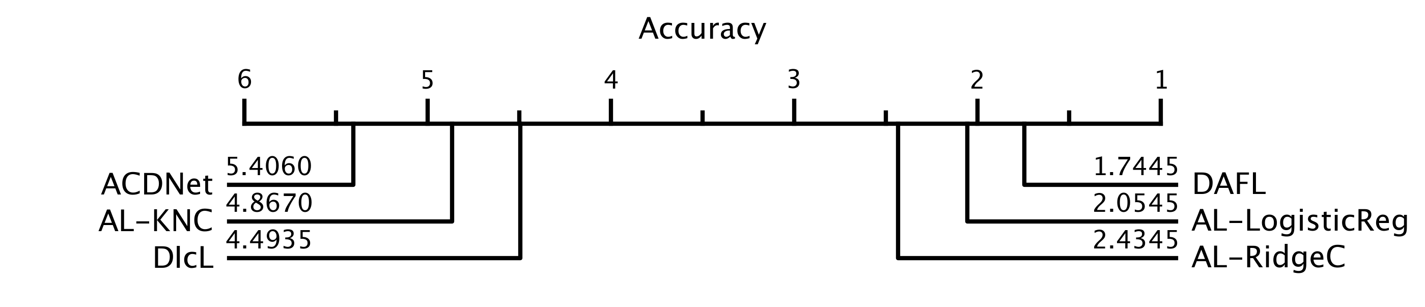
Figure 16: CD diagram showing statistical significance of the learning methods on the ESC-50 dataset.

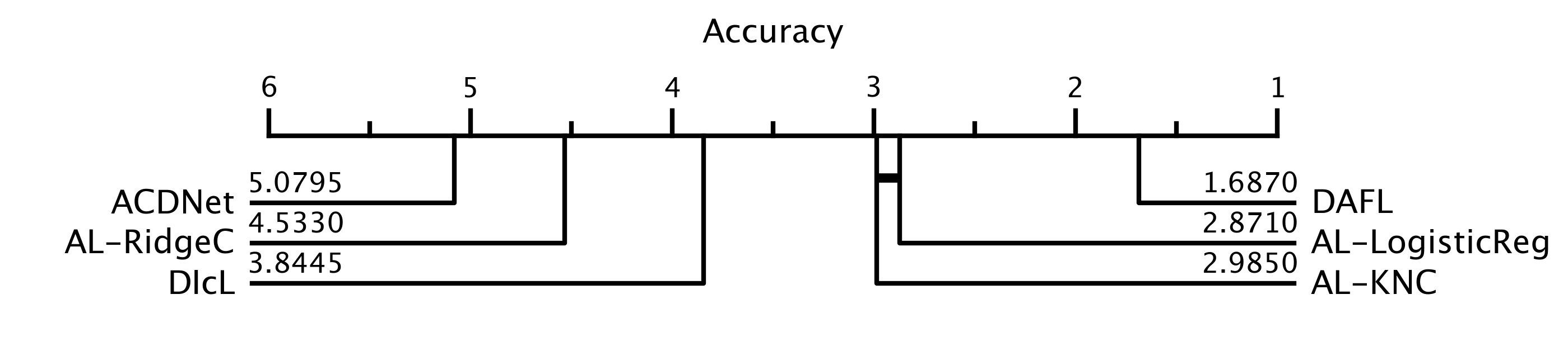
Figure 17: CD diagram showing statistical significance of the learning methods on the US8K dataset.

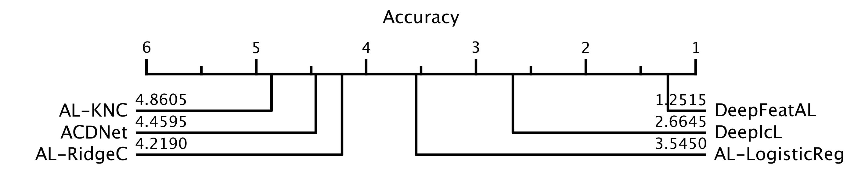
Figure 18: CD diagram showing statistical significance of the learning methods on iWingBeat dataset.

5 Real-world Application

To test the practical relevance of our method, we apply DAFL to data from a real-world conservation study. The objective is to identify the calls of an endangered subspecies of the Black-throated Finch (BTF) (Poephila cincta cincta [57] found in Queensland, Australia) [57] from audio recorded in the wild with standard bio-acoustic recorders.

The dataset consists of 49 files containing 98h of continuous audio recorded at 44.1kHz with 16-bit resolution ($\approx$2h per file). Calls were manually annotated by human experts and used to train and test an ACDnet model for the automated labelling of future recordings. A total of 2907 BTF calls were labelled. Unlabelled data in the recordings consists of calls from various other species and environmental background sounds (BGS).

Our review of the labelled data showed that the length of typical calls ranges from 0.6s to 0.672s. Consequently, we used sliding time windows of 0.6s length with a 0.1s offset for continuous recognition. Each sample is thus a vector $x_{i}\in\mathbb{R}^{12}$ (0.6s x 20,000Hz). We used zero padding at the end for windows that did not yield 12,000 data points. We augmented all BTF samples using adding noise, time-stretching, pitch-shifting, and time-shifting to obtain 20,000 samples. We regarded a window as a positive sample if it had at least 50% overlap with a BTF annotation. Full details of the data sets are given in Table 3.

Datasets	Recording time (h)	#Files	#Samples	Actual BTF Calls	Overlapping BTF Samples	BGS Samples	Augmented BTF Samples
Training set	80	40	410,349	2,602	10,349	4000,000	9,651
Validation set	6	3	30,787	198	787	30,000	-
Test set	12	6	432,000	107	426	431,576	-

Table 3: Training set, validation set and test set details

It is important to consider the exact nature of the real-world task as this has important implications for how performance must be measured. The objective is not to classify individual calls or to detect and/or count every individual call in the recordings. Rather, the real-world task is the detection of sites at which the target species is present. In a sense, the real task is the binary classification of sites, not sounds, according to the presence and absence of the target species. This site classification needs to be achieved with high accuracy and, importantly, with as little human intervention as possible.

Since reliable site classification is required, verification by a human expert as a post-process cannot be avoided. This implies that a simple sliding time-window recognition as described above cannot be used naïvely: it will produce too many false positives, necessitating too much manual checking. Even assuming an (unrealistically high) 95% raw classification accuracy, naïve application would produce more than 20,000 false positives per day (assuming equal rates of false positives and false negatives). It is impossible for a human expert to classify a 0.6s time window reliably in isolation. Rather, calls have to be listened to in a minimal temporal context (from experience, we assume 2 seconds). This means that 20,000 potential false positives amount to more than 11h human post-processing, so not much would be gained at all from such an approach compared to direct listening.

To overcome this problem, we exploit the fact that calls generally occur in clusters if they are present at all. As we only need site classification, we can afford to miss most calls at a site, as long as we do not miss all calls. In theory, a single reliably identified call is enough to classify the site positively. This allows us to circumvent the above problem by strongly biasing our classifier towards false negatives and summarizing the recognition in longer segments for human checking.

Based on an analysis of the call structures we decided to work with 5-second audio segments that were classified if they contained at least 4 recognized time slices. Biasing towards false negatives was induced using training class imbalance (see Table 3).

Table 4 and Table 5 present the results of applying ACDNet and Micro-ACDNet to the test data with this post-process. As each test file produced more than zero true positives (with the exception of Test File 5, which contains no calls), 100% of the occupied sites would have been correctly detected by combing the automatic classification with human checking of just the positively classified segments (TP+FP). The effort for post-processing is determined by the number of these segments. ACD (Micro-ACDnet) produced a total of 21 TP and 8 FP (16 TP and 14 FP), respectively, for the whole test set. This amounts to ca. 2.5 minutes of human verification (in 5-second chunks) required for the whole 12-hour test data set, or equivalently less than 5 minutes per day—a very feasible amount. In practice, even less effort may be required, as the verification can be stopped as soon as the first positive sample has been verified with certainty.

Test File No.	#5s Segments	#BTF Call Segments	TP	FP	FN	TN
1	1440	7	5	0	2	1433
2	1440	16	2	1	14	1423
3	1440	12	3	1	9	1427
4	1440	23	6	2	17	1415
5	1440	0	0	1	0	1439
6	1440	13	5	3	8	1424
Total	8,640	71	21	8	50	8,561

Table 4: Results after post-processing of the predictions from ACDNet

Test File No.	#5s Segments	#BTF Call Segments	TP	FP	FN	TN
1	1440	7	4	0	3	1433
2	1440	16	2	3	14	1421
3	1440	12	1	1	11	1427
4	1440	23	4	4	19	1413
5	1440	0	0	1	0	1439
6	1440	13	5	5	8	1422
Total	8,640	71	16	14	55	8,555

Table 5: Results after post-processing of the predictions from Micro-ACDNet

We now evaluate the relevance of the proposed DAFL schema in the context of this application. The full model reported above was trained on 80 hours of recordings that were manually labelled by a human expert (Table 3). We apply DAFL to reduce these labelling requirements. Initially, we use only 50% of the training recordings to train a Micro-ACDnet. This equates to 40 hours of labelling effort. We then run 10 rounds of active learning. In each round, the algorithm queries the expert to label 1,000 samples selected by the active learning procedure. If we assume a 2-second context for the presentation of each sample, as above, this equates to ca. 33 minutes of labelling time per active learning iteration or 5.5 hours for all ten iterations.

The performance of the DAFL-trained Micro-ACDnet model is fully comparable to the full-sized ACDnet model trained on the entire training set. Table 6 shows the performance of the model after each round of active learning. The last two columns show how many samples from the 1,000 sample training batch presented by the algorithm in the specific training round are correctly classified before and after the re-training. To confirm that the increase in performance is indeed caused by the active learning and not just by further training epochs, we compare the active learning performance to the performance of the model trained on just the initial training set for the same additional number of epochs in every round (column “retraining”). The model performing best in terms of overall precision is kept as the final trained model (Iteration 5).

Table 7 details the test performance of the final model for the six individual test files including post-processing as described above. We see that the number of true positives and false negatives is approximately equivalent to the full ACDnet model (Table 4). Likewise, the number of true positives plus false positives, which determines the total amount of human post-processing, differs only marginally (29 for the fully trained ACDnet versus 36 for the actively trained Micro-ACDnet).

Overall, the DAFL procedure allowed us to reduce the total labelling time required for training by 43% from 80 hours to 45.5 hours while maintaining the same performance (in terms of human post-processing required for full detection accuracy). It did so while allowing us to simultaneously transition from a large model to a small one suitable for edge devices. This demonstrates the practical relevance of the proposed DAFL.

Learning Iteration	#5s Segments	#BTF Call Segments	Retraining			DAFL
									1,000 Annotated Samples
			TP	FP	Precision	TP	FP	Precision	Known Before retrain ing	Known After retrain ing
0	8,640	71	15	15	0.50	15	15	0.50	-	-
1	8,640	71	19	22	0.46	21	21	0.50	646	730
2	8,640	71	21	38	0.36	19	18	0.51	655	767
3	8,640	71	21	47	0.31	17	20	0.46	709	747
4	8,640	71	19	23	0.45	21	24	0.47	787	799
5	8,640	71	22	34	0.39	19	17	0.53	775	818
6	8,640	71	23	49	0.32	14	17	0.45	790	845
7	8,640	71	22	39	0.36	16	22	0.42	803	819
8	8,640	71	22	57	0.28	13	20	0.39	780	766
9	8,640	71	23	53	0.30	18	42	0.30	799	819
10	8,640	71	18	22	0.45	14	20	0.41	785	798

Table 6: Performance of Micro-ACDnet for 10 rounds of active learning.

Test File No.	#5s Segments	#BTF Call Segments	TP	FP	FN	TN
1	1440	7	4	1	3	1432
2	1440	16	3	4	13	1420
3	1440	12	1	2	11	1426
4	1440	23	7	4	16	1412
5	1440	0	0	1	0	1439
6	1440	13	4	5	9	1422
Total	8,640	71	19	17	52	8,551

Table 7: Performance of the best Micro-ACDnet model for each test file.

6 Conclusion

Our study was designed to test the hypothesis that including feature extraction in the Active Learning loop provides performance benefits in (bio)acoustic classification. Our experimental investigation on three widely used standard benchmark datasets (ESC-50, US8K, and iWingBeat) as well as on real-world data provides clear and statistically significant evidence to confirm this hypothesis.

Integrating and fine-tuning the feature extractor into the AL loop allows faster learning and thus enables us to either reach a set accuracy level with a smaller labelling budget or to reach higher accuracy with a fixed labelling budget.

The proposed method was tested with a large standard model and with a very small model suitable for edge-AI applications. It provided similar performance benefits in both cases. This should pave the way for the use of active learning in edge devices.

In the future, we plan to investigate integrated edge-AI architectures in which the edge devices autonomously collect new samples and send these “back to base” for expert labelling. The hope is that this will provide a useful approach for edge-AI devices that can continuously learn and improve their performance in the field.

7 Appendix

7.1 Experimental Details

All experiments were conducted using Python version 3.7.4 and PyTorch 1.8.1.

7.1.1 Datasets

Experiments were carried out on three popular audio benchmark datasets: ESC-50 [36], US8K [18] and iWingBeat [19]. ESC-50 contains 2,000 samples, each of which is a 5-second audio recording sampled at 16kHz and 44.1kHz and distributed evenly among 50 balanced, separate classes (40 audio samples for each class). To achieve reproducible results, a presorted partition into 5 folds is also available for 5-fold cross-validation. The US8K dataset contains 8,732 labelled audio clips (of 4-second length) of urban sounds recorded at 22.05kHz from 10 classes. The clips are grouped into 10 folds for cross-validating the results for fair comparison. The iWingBeat dataset includes 50,000 labelled audio clips (length of 1 second each) from 10 classes of insects, with 5,000 examples per class. We resampled all audio samples of all datasets to 20kHz.

7.1.2 Splitting the Datasets for DeepIcL, Standard AL and DeepFeatAL

We separate the datasets into two parts. One is used for training, validation, and testing, while the data from the second part are placed in an unlabeled data pool. We keep 50%, 50% and 35% data instances from every class of the datasets for training, validation and testing.

We then create training sets, validation sets and test sets with 40%, 20% and 40% of the reserved data (for training, validation and testing) of the ESC-50 dataset, 40%, 20% and 40% of the US8K dataset and 57%, 28.5% and 28.5% of the iWingBeat dataset, respectively.

Finally, we move the remaining data to the unlabeled data pool.

7.1.3 Data Preprocessing

For ESC-50 and US8K, we follow the procedure described in [20]. For the iWingBeat dataset, we use input samples of length 20,000, or 1s audio at 20kHz since the recordings are only 1s long. We use the data augmentation techniques described in Mohaimenuzzaman et al. [20] and Mohaimenuzzaman et al. [21] to augment the training sets of the ESC-50, US8K and iWingBeat datasets. However, we do not employ the mixup of two classes for the training set augmentation and 10-crops of test data proposed in those articles because our goal is to improve model learning via active learning rather than those strategies.

7.1.4 Hyperparameter Settings for Initial Training

ACDNet is trained for 600 epochs with a learning rate scheduler 0.3, 0.6, 0.9 with the same learning settings described in Mohaimenuzzaman et al. [20]. At the end of training and validation, we use the best model for testing, DIcL, DAL and DAFL.

7.1.5 Learning Settings for DeepIcl, Standard AL and DeepFeatAL

We use seven, fifteen, and twenty iterations of human annotation (simulated) on the ESC-50, US8K, and iWingBeat datasets, respectively. In each iteration, the simulated annotation system is requested to provide the labels of 100 specific unlabeled samples (determined by the acquisition function) for the first two datasets and 500 unlabeled samples for the third dataset. In each iteration of the simulated labelling, we fine-tune the model for 100 epochs for each dataset during DIcL and DAFL; however, we add the same number of old training data to the newly labelled data to prevent the network from forgetting its prior knowledge. During this stage of learning with new data, we employ a significantly lower learning rate (i.e., 0.001), a new learning rate scheduler of [15, 60, 90] without any warm-ups and a batch size of 16.

7.2 Additional Tables Representing Experimental Results

The outcomes of all three steps of fine-tuning are provided in Table 8. In learning loops 1-7, the model was fine-tune d with 100 new data instances.

	Prediction Accuracy (%)
Learning Loops	No-freeze	Fixed-freeze	Scheduled-freeze
0	55.75	55.75	55.75
1	59.50	58.00	59.50
2	61.25	59.25	60.75
3	61.75	59.75	61.25
4	64.00	62.00	63.00
5	63.50	62.50	62.00
6	64.75	62.75	63.75
7	65.50	63.50	64.00

Table 8: ACDNet in different training settings for incremental Learning. The first row indicates the performance of the model before incremental learning.

	Accuracy(95%CI)
Learning Loops	DIcL	AL-KNC	AL-LogisticReg	AL-RidgeC
0	55.81 $\pm$ 0.15	54.02 $\pm$ 0.15	58.78 $\pm$ 0.15	57.79 $\pm$ 0.16
1	59.56 $\pm$ 0.15	56.83 $\pm$ 0.14	60.76 $\pm$ 0.16	59.54 $\pm$ 0.14
2	61.23 $\pm$ 0.15	61.19 $\pm$ 0.15	63.19 $\pm$ 0.15	62.58 $\pm$ 0.15
3	61.71 $\pm$ 0.15	62.73 $\pm$ 0.15	63.81 $\pm$ 0.16	65.19 $\pm$ 0.14
4	63.94 $\pm$ 0.15	63.19 $\pm$ 0.14	64.04 $\pm$ 0.15	67.00 $\pm$ 0.15
5	63.38 $\pm$ 0.15	63.22 $\pm$ 0.15	65.46 $\pm$ 0.15	67.10 $\pm$ 0.15
6	64.69 $\pm$ 0.15	64.86 $\pm$ 0.14	64.50 $\pm$ 0.15	67.73 $\pm$ 0.15
7	65.43 $\pm$ 0.15	65.18 $\pm$ 0.15	66.77 $\pm$ 0.15	67.94 $\pm$ 0.14

Table 9: DIcL vs DAL using ACDNet on ESC-50 dataset

	Accuracy (95%CI)
Learning Loops	DIcL	AL-KNC	AL-LogisticReg	AL-RidgeC
0	86.97 $\pm$ 0.06	87.24 $\pm$ 0.05	87.55 $\pm$ 0.05	87.00 $\pm$ 0.05
1	87.12 $\pm$ 0.05	87.60 $\pm$ 0.05	87.48 $\pm$ 0.05	86.80 $\pm$ 0.05
2	86.94 $\pm$ 0.04	87.51 $\pm$ 0.05	88.25 $\pm$ 0.04	87.09 $\pm$ 0.05
3	87.47 $\pm$ 0.06	87.49 $\pm$ 0.05	88.08 $\pm$ 0.04	87.60 $\pm$ 0.04
4	87.46 $\pm$ 0.05	87.66 $\pm$ 0.05	88.00 $\pm$ 0.05	87.42 $\pm$ 0.05
5	87.98 $\pm$ 0.04	87.65 $\pm$ 0.04	87.96 $\pm$ 0.05	87.27 $\pm$ 0.06
6	87.80 $\pm$ 0.05	88.05 $\pm$ 0.05	87.96 $\pm$ 0.05	87.38 $\pm$ 0.05
7	87.78 $\pm$ 0.06	88.14 $\pm$ 0.05	87.79 $\pm$ 0.05	87.47 $\pm$ 0.04
8	87.94 $\pm$ 0.05	88.12 $\pm$ 0.04	88.08 $\pm$ 0.04	87.54 $\pm$ 0.05
9	86.91 $\pm$ 0.05	88.04 $\pm$ 0.05	88.16 $\pm$ 0.05	87.49 $\pm$ 0.05
10	87.67 $\pm$ 0.05	87.93 $\pm$ 0.05	88.25 $\pm$ 0.04	87.72 $\pm$ 0.04
11	88.19 $\pm$ 0.06	88.05 $\pm$ 0.05	88.18 $\pm$ 0.05	87.70 $\pm$ 0.06
12	87.67 $\pm$ 0.05	87.91 $\pm$ 0.05	88.21 $\pm$ 0.05	87.73 $\pm$ 0.05
13	87.00 $\pm$ 0.04	87.80 $\pm$ 0.05	88.48 $\pm$ 0.06	87.80 $\pm$ 0.05
14	86.71 $\pm$ 0.06	88.18 $\pm$ 0.05	88.17 $\pm$ 0.05	87.78 $\pm$ 0.05
15	87.38 $\pm$ 0.04	88.48 $\pm$ 0.05	88.31 $\pm$ 0.05	87.82 $\pm$ 0.05

Table 10: DIcL vs DAL on US8K dataset

	Accuracy (95%CI)
Learning Loops	DIcL	AL-KNC	AL-LogisticReg	AL-RidgeC
0	66.08 $\pm$ 0.04	66.31 $\pm$ 0.04	66.11 $\pm$ 0.04	65.82 $\pm$ 0.04
1	66.94 $\pm$ 0.04	66.31 $\pm$ 0.04	66.53 $\pm$ 0.04	65.79 $\pm$ 0.04
2	66.50 $\pm$ 0.04	66.47 $\pm$ 0.04	66.57 $\pm$ 0.04	65.95 $\pm$ 0.04
3	66.21 $\pm$ 0.04	66.61 $\pm$ 0.04	66.53 $\pm$ 0.04	66.02 $\pm$ 0.04
4	66.63 $\pm$ 0.04	66.44 $\pm$ 0.04	66.64 $\pm$ 0.04	65.89 $\pm$ 0.04
5	67.19 $\pm$ 0.04	66.22 $\pm$ 0.04	66.61 $\pm$ 0.04	65.87 $\pm$ 0.04
6	67.30 $\pm$ 0.04	66.17 $\pm$ 0.04	66.68 $\pm$ 0.04	66.03 $\pm$ 0.04
7	67.79 $\pm$ 0.04	66.19 $\pm$ 0.04	66.79 $\pm$ 0.04	66.01 $\pm$ 0.04
8	67.11 $\pm$ 0.04	66.29 $\pm$ 0.04	66.91 $\pm$ 0.04	66.14 $\pm$ 0.04
9	67.32 $\pm$ 0.04	66.28 $\pm$ 0.04	66.95 $\pm$ 0.04	66.04 $\pm$ 0.04
10	67.20 $\pm$ 0.04	66.14 $\pm$ 0.04	67.02 $\pm$ 0.04	66.16 $\pm$ 0.04
11	67.97 $\pm$ 0.04	66.24 $\pm$ 0.04	67.15 $\pm$ 0.04	66.12 $\pm$ 0.04
12	67.07 $\pm$ 0.04	66.15 $\pm$ 0.04	67.05 $\pm$ 0.04	66.36 $\pm$ 0.04
13	67.27 $\pm$ 0.04	66.22 $\pm$ 0.04	67.10 $\pm$ 0.04	66.32 $\pm$ 0.04
14	66.66 $\pm$ 0.04	66.35 $\pm$ 0.04	67.10 $\pm$ 0.04	66.20 $\pm$ 0.04
15	67.54 $\pm$ 0.04	66.35 $\pm$ 0.04	67.03 $\pm$ 0.04	66.14 $\pm$ 0.04
16	67.50 $\pm$ 0.04	66.43 $\pm$ 0.04	67.13 $\pm$ 0.04	66.25 $\pm$ 0.04
17	67.65 $\pm$ 0.04	66.10 $\pm$ 0.04	67.17 $\pm$ 0.04	66.31 $\pm$ 0.04
18	67.62 $\pm$ 0.04	66.11 $\pm$ 0.04	67.17 $\pm$ 0.04	66.37 $\pm$ 0.04
19	68.27 $\pm$ 0.04	66.03 $\pm$ 0.04	67.11 $\pm$ 0.04	66.30 $\pm$ 0.04
20	68.16 $\pm$ 0.04	65.87 $\pm$ 0.04	67.17 $\pm$ 0.04	66.28 $\pm$ 0.04

Table 11: DIcL vs DAL on iWingBeat dataset

	Accuracy(95%CI)
Learning Loops	DIcL	AL-KNC	AL-LogisticReg	AL-RidgeC
0	55.36 $\pm$ 0.14	47.89 $\pm$ 0.15	52.67 $\pm$ 0.15	52.46 $\pm$ 0.16
1	55.99 $\pm$ 0.15	48.89 $\pm$ 0.14	56.08 $\pm$ 0.16	53.89 $\pm$ 0.14
2	55.72 $\pm$ 0.15	53.80 $\pm$ 0.15	56.47 $\pm$ 0.15	58.09 $\pm$ 0.15
3	55.24 $\pm$ 0.15	55.35 $\pm$ 0.15	60.25 $\pm$ 0.16	61.53 $\pm$ 0.14
4	56.25 $\pm$ 0.15	58.83 $\pm$ 0.14	60.25 $\pm$ 0.15	61.16 $\pm$ 0.15
5	54.94 $\pm$ 0.15	57.37 $\pm$ 0.15	62.76 $\pm$ 0.15	61.20 $\pm$ 0.15
6	57.37 $\pm$ 0.15	57.92 $\pm$ 0.14	62.70 $\pm$ 0.15	60.70 $\pm$ 0.15
7	57.70 $\pm$ 0.15	56.67 $\pm$ 0.15	63.32 $\pm$ 0.15	62.38 $\pm$ 0.14

Table 12: Edge-based DIcL vs DAL on ESC-50 dataset

	Accuracy (95%CI)
Learning Loops	DIcL	AL-KNC	AL-LogisticReg	AL-RidgeC
0	81.71 $\pm$ 0.06	81.77 $\pm$ 0.06	82.79 $\pm$ 0.06	81.84 $\pm$ 0.06
1	81.73 $\pm$ 0.06	82.06 $\pm$ 0.06	82.70 $\pm$ 0.06	81.71 $\pm$ 0.06
2	81.41 $\pm$ 0.06	82.16 $\pm$ 0.06	82.70 $\pm$ 0.06	82.02 $\pm$ 0.05
3	82.57 $\pm$ 0.06	82.36 $\pm$ 0.06	82.92 $\pm$ 0.06	82.26 $\pm$ 0.06
4	82.70 $\pm$ 0.06	82.44 $\pm$ 0.06	82.85 $\pm$ 0.06	81.92 $\pm$ 0.06
5	83.13 $\pm$ 0.06	82.20 $\pm$ 0.06	83.09 $\pm$ 0.06	82.04 $\pm$ 0.06
6	82.34 $\pm$ 0.06	82.35 $\pm$ 0.06	83.11 $\pm$ 0.06	81.98 $\pm$ 0.06
7	82.98 $\pm$ 0.06	82.85 $\pm$ 0.06	82.79 $\pm$ 0.06	82.12 $\pm$ 0.06
8	82.76 $\pm$ 0.06	82.80 $\pm$ 0.06	83.11 $\pm$ 0.06	81.96 $\pm$ 0.06
9	82.10 $\pm$ 0.06	82.77 $\pm$ 0.06	83.18 $\pm$ 0.06	82.01 $\pm$ 0.06
10	82.36 $\pm$ 0.06	82.66 $\pm$ 0.06	83.10 $\pm$ 0.06	82.25 $\pm$ 0.06
11	82.33 $\pm$ 0.06	83.02 $\pm$ 0.06	83.17 $\pm$ 0.06	82.16 $\pm$ 0.06
12	82.51 $\pm$ 0.06	83.30 $\pm$ 0.06	83.38 $\pm$ 0.06	82.01 $\pm$ 0.06
13	82.80 $\pm$ 0.06	83.24 $\pm$ 0.06	83.19 $\pm$ 0.06	82.15 $\pm$ 0.06
14	82.64 $\pm$ 0.06	82.97 $\pm$ 0.06	83.20 $\pm$ 0.06	81.89 $\pm$ 0.06
15	82.63 $\pm$ 0.06	83.15 $\pm$ 0.06	83.27 $\pm$ 0.06	82.16 $\pm$ 0.06

Table 13: Edge-based DIcL vs DAL on US8K dataset

	Accuracy (95%CI)
Learning Loops	DIcL	AL-KNC	AL-LogisticReg	AL-RidgeC
0	62.51 $\pm$ 0.04	62.59 $\pm$ 0.04	62.70 $\pm$ 0.04	62.29 $\pm$ 0.04
1	62.51 $\pm$ 0.05	62.54 $\pm$ 0.04	62.46 $\pm$ 0.04	62.16 $\pm$ 0.04
2	63.00 $\pm$ 0.05	62.54 $\pm$ 0.04	62.72 $\pm$ 0.04	62.22 $\pm$ 0.04
3	63.09 $\pm$ 0.04	62.20 $\pm$ 0.04	62.61 $\pm$ 0.04	62.22 $\pm$ 0.04
4	62.77 $\pm$ 0.04	62.33 $\pm$ 0.04	62.72 $\pm$ 0.04	62.24 $\pm$ 0.04
5	63.04 $\pm$ 0.04	62.20 $\pm$ 0.04	62.73 $\pm$ 0.04	62.17 $\pm$ 0.04
6	63.45 $\pm$ 0.05	62.55 $\pm$ 0.04	62.62 $\pm$ 0.04	62.27 $\pm$ 0.04
7	63.29 $\pm$ 0.04	62.66 $\pm$ 0.04	62.76 $\pm$ 0.04	62.38 $\pm$ 0.04
8	63.64 $\pm$ 0.04	62.67 $\pm$ 0.04	62.73 $\pm$ 0.04	62.39 $\pm$ 0.04
9	63.35 $\pm$ 0.04	62.92 $\pm$ 0.04	62.96 $\pm$ 0.04	62.39 $\pm$ 0.04
10	63.59 $\pm$ 0.04	62.96 $\pm$ 0.04	62.93 $\pm$ 0.04	62.48 $\pm$ 0.04
11	63.88 $\pm$ 0.04	62.85 $\pm$ 0.04	62.89 $\pm$ 0.04	62.59 $\pm$ 0.04
12	63.09 $\pm$ 0.05	63.12 $\pm$ 0.04	63.03 $\pm$ 0.04	62.62 $\pm$ 0.04
13	63.20 $\pm$ 0.05	62.81 $\pm$ 0.04	62.88 $\pm$ 0.04	62.49 $\pm$ 0.04
14	62.64 $\pm$ 0.05	62.72 $\pm$ 0.04	62.96 $\pm$ 0.04	62.59 $\pm$ 0.04
15	63.80 $\pm$ 0.04	62.81 $\pm$ 0.04	62.95 $\pm$ 0.04	62.52 $\pm$ 0.04
16	63.56 $\pm$ 0.04	62.43 $\pm$ 0.04	62.96 $\pm$ 0.04	62.57 $\pm$ 0.04
17	63.72 $\pm$ 0.04	62.17 $\pm$ 0.04	63.03 $\pm$ 0.04	62.61 $\pm$ 0.04
18	63.79 $\pm$ 0.04	62.23 $\pm$ 0.04	62.96 $\pm$ 0.04	62.66 $\pm$ 0.04
19	63.47 $\pm$ 0.04	62.33 $\pm$ 0.04	62.99 $\pm$ 0.04	62.70 $\pm$ 0.04
20	63.42 $\pm$ 0.04	62.27 $\pm$ 0.04	63.01 $\pm$ 0.04	62.63 $\pm$ 0.04

Table 14: Edge-based DIcL vs DAL on iWingBeat dataset

References

- Ren et al. [2021] Pengzhen Ren, Yun Xiao, Xiaojun Chang, Po-Yao Huang, Zhihui Li, Brij B Gupta, Xiaojiang Chen, and Xin Wang. A survey of deep active learning. ACM Computing Surveys (CSUR), 54(9):1–40, 2021.
- Ash et al. [2019] Jordan T Ash, Chicheng Zhang, Akshay Krishnamurthy, John Langford, and Alekh Agarwal. Deep batch active learning by diverse, uncertain gradient lower bounds. In International Conference on Learning Representations, ICLR 2019, 2019.
- Han et al. [2016] Wenjing Han, Eduardo Coutinho, Huabin Ruan, Haifeng Li, Björn Schuller, Xiaojie Yu, and Xuan Zhu. Semi-supervised active learning for sound classification in hybrid learning environments. PloS one, 11(9):e0162075, 2016.
- Settles [2012] Burr Settles. Active learning. Synthesis lectures on artificial intelligence and machine learning, 6(1):1–114, 2012.
- Coleman et al. [2020] William Coleman, Charlie Cullen, Ming Yan, and Sarah Jane Delany. Active learning for auditory hierarchy. In Proceedings of the International Cross-Domain Conference for Machine Learning and Knowledge Extraction, 2020, pages 365–384. Springer, 2020.
- Hilasaca et al. [2021] Liz Huancapaza Hilasaca, Milton Cezar Ribeiro, and Rosane Minghim. Visual active learning for labeling: A case for soundscape ecology data. Information, 12(7):265, 2021.
- Roy and McCallum [2001] Nicholas Roy and Andrew McCallum. Toward optimal active learning through Monte Carlo estimation of error reduction. ICML, Williamstown, 2:441–448, 2001.
- Shuyang et al. [2017] Zhao Shuyang, Toni Heittola, and Tuomas Virtanen. Active learning for sound event classification by clustering unlabeled data. In Proceedings of the IEEE International Conference on Acoustics, Speech and Signal Processing, ICASSP 2017, pages 751–755. IEEE, 2017.
- Qian et al. [2017] Kun Qian, Zixing Zhang, Alice Baird, and Björn Schuller. Active learning for bird sound classification via a kernel-based extreme learning machine. The Journal of the Acoustical Society of America, 142(4):1796–1804, 2017.
- Kholghi et al. [2018] Mahnoosh Kholghi, Yvonne Phillips, Michael Towsey, Laurianne Sitbon, and Paul Roe. Active learning for classifying long-duration audio recordings of the environment. Methods in Ecology and Evolution, 9(9):1948–1958, 2018.
- Shuyang et al. [2018] Zhao Shuyang, Toni Heittola, and Tuomas Virtanen. An active learning method using clustering and committee-based sample selection for sound event classification. In Proceedings of the 16th International Workshop on Acoustic Signal Enhancement, IWAENC 2018, pages 116–120. IEEE, 2018.
- Qin et al. [2019] Xiao Qin, Wanting Ji, Ruili Wang, and ChangAn Yuan. Learnt dictionary based active learning method for environmental sound event tagging. Multimedia Tools and Applications, 78(20):29493–29508, 2019.
- Wang et al. [2019] Yu Wang, Ana Elisa Mendez Mendez, Mark Cartwright, and Juan Pablo Bello. Active learning for efficient audio annotation and classification with a large amount of unlabeled data. In Proceedings of the IEEE international conference on acoustics, speech and signal processing, ICASSP 2019, pages 880–884. IEEE, 2019.
- Ji et al. [2019] Wanting Ji, Ruili Wang, and Junbo Ma. Dictionary-based active learning for sound event classification. Multimedia tools and applications, 78(3):3831–3842, 2019.
- Shuyang et al. [2020] Zhao Shuyang, Toni Heittola, and Tuomas Virtanen. Active learning for sound event detection. IEEE/ACM Transactions on Audio, Speech, and Language Processing, 28:2895–2905, 2020.
- Shi et al. [2020] Haotian Shi, Haoren Wang, Chengjin Qin, Liqun Zhao, and Chengliang Liu. An incremental learning system for atrial fibrillation detection based on transfer learning and active learning. Computer methods and programs in biomedicine, 187:105219, 2020.
- Piczak [2017] Karol Piczak. ESC-50: Dataset for environmental sound classification. https://github.com/karolpiczak/ESC-50, 2017.
- Salamon et al. [2014] Justin Salamon, Christopher Jacoby, and Juan Pablo Bello. A dataset and taxonomy for urban sound research. In Proceedings of the 22nd ACM international conference on Multimedia, 2014, pages 1041–1044. ACM, 2014.
- Chen et al. [2014] Yanping Chen, Adena Why, Gustavo Batista, Agenor Mafra-Neto, and Eamonn Keogh. Flying insect classification with inexpensive sensors. Journal of insect behavior, 27(5):657–677, 2014.
- Mohaimenuzzaman et al. [2023] Md Mohaimenuzzaman, Christoph Bergmeir, Ian West, and Bernd Meyer. Environmental sound classification on the edge: A pipeline for deep acoustic networks on extremely resource-constrained devices. Pattern Recognition, 133:109025, 2023.
- Mohaimenuzzaman et al. [2022] Md Mohaimenuzzaman, Christoph Bergmeir, and Bernd Meyer. Pruning vs XNOR-Net: A comprehensive study of deep learning for audio classification on edge-devices. IEEE Access, 10:6696–6707, 2022.
- Tokozume and Harada [2017] Yuji Tokozume and Tatsuya Harada. Learning environmental sounds with end-to-end convolutional neural network. In Proceedings of the IEEE International Conference on Acoustics, Speech and Signal Processing, ICASSP 2017, pages 2721–2725. IEEE, 2017.
- Tokozume et al. [2018] Yuji Tokozume, Yoshitaka Ushiku, and Tatsuya Harada. Learning from between-class examples for deep sound recognition. In Proceedings of the 6th International Conference on Learning Representations, ICLR 2018, page https://openreview.net/forum?id=B1Gi6LeRZ. OpenReview.net, 2018.
- Huang and Leanos [2018] Jonathan J Huang and Juan Jose Alvarado Leanos. AclNet: efficient end-to-end audio classification CNN. arXiv preprint arXiv:1811.06669, 2018.
- Hershey et al. [2017] Shawn Hershey, Sourish Chaudhuri, Daniel PW Ellis, Jort F Gemmeke, Aren Jansen, R Channing Moore, Manoj Plakal, Devin Platt, Rif A Saurous, Bryan Seybold, et al. CNN architectures for large-scale audio classification. In Proceedings of the IEEE international conference on acoustics, speech and signal processing, ICASSP 2017, pages 131–135. IEEE, 2017.
- Schröder et al. [2016] Jens Schröder, Jorn Anemuller, and Stefan Goetze. Classification of human cough signals using spectro-temporal Gabor filterbank features. In Proceedings of the IEEE International Conference on Acoustics, Speech and Signal Processing, ICASSP 2016, pages 6455–6459. IEEE, 2016.
- Eyben et al. [2010] Florian Eyben, Martin Wöllmer, and Björn Schuller. OpenSmile: the munich versatile and fast open-source audio feature extractor. In Proceedings of the 18th International Conference on Multimedia, 2010, pages 1459–1462, 2010.
- Breiman [2001] Leo Breiman. Random forests. Machine learning, 45(1):5–32, 2001.
- Cortes and Vapnik [1995] Corinna Cortes and Vladimir Vapnik. Support-vector networks. Machine learning, 20(3):273–297, 1995.
- Fix and Hodges [1989] Evelyn Fix and Joseph Lawson Hodges. Discriminatory analysis. nonparametric discrimination: Consistency properties. International Statistical Review/Revue Internationale de Statistique, 57(3):238–247, 1989.
- Cox [1958] David R Cox. The regression analysis of binary sequences. Journal of the Royal Statistical Society: Series B (Methodological), 20(2):215–232, 1958.
- Lewis and Gale [1994] David D Lewis and William A Gale. A sequential algorithm for training text classifiers. In Proceedings of the 17th Annual International ACM-SIGIR Conference on Research and Development in Information Retrieval, SIGIR 1994, pages 3–12. ACM/Springer, 1994.
- Basu et al. [2004] Sugato Basu, Arindam Banerjee, and Raymond J Mooney. Active semi-supervision for pairwise constrained clustering. In Proceedings of the 4th SIAM International Conference on Data Mining, 2004, pages 333–344. SIAM, 2004.
- Seung et al. [1992] H Sebastian Seung, Manfred Opper, and Haim Sompolinsky. Query by committee. In Proceedings of the 5th annual workshop on Computational learning theory, 1992, pages 287–294, 1992.
- FindSounds [2017] FindSounds. Sound types. https://findsounds.com/types.html, 2017.
- Piczak [2015] Karol J. Piczak. ESC: Dataset for environmental sound classification. In Proceedings of the 23rd Annual ACM Conference on Multimedia, 2015, pages 1015–1018. ACM Press, 2015. ISBN 978-1-4503-3459-4. doi: 10.1145/2733373.2806390. URL http://dl.acm.org/citation.cfm?doid=2733373.2806390.
- Vassilvitskii and Arthur [2006] Sergei Vassilvitskii and David Arthur. k-means++: The advantages of careful seeding. In Proceedings of the eighteenth annual ACM-SIAM symposium on Discrete algorithms, pages 1027–1035, 2006.
- Kim and Pardo [2017] Bongjun Kim and Bryan Pardo. I-SED: An interactive sound event detector. In Proceedings of the 22nd International Conference on Intelligent User Interfaces, 2017, pages 553–557, 2017.
- Kim and Pardo [2018] Bongjun Kim and Bryan Pardo. A human-in-the-loop system for sound event detection and annotation. ACM Transactions on Interactive Intelligent Systems (TiiS), 8(2):1–23, 2018.
- Stowell et al. [2015] Dan Stowell, Dimitrios Giannoulis, Emmanouil Benetos, Mathieu Lagrange, and Mark D Plumbley. Detection and classification of acoustic scenes and events. IEEE Transactions on Multimedia, 17(10):1733–1746, 2015.
- Mesaros et al. [2017] Annamaria Mesaros, Toni Heittola, Aleksandr Diment, Benjamin Elizalde, Ankit Shah, Emmanuel Vincent, Bhiksha Raj, and Tuomas Virtanen. DCASE 2017 challenge setup: Tasks, datasets and baseline system. In Proceedings of the Detection and Classification of Acoustic Scenes and Events Workshop, DCASE 2017, 2017.
- Turpault et al. [2019] Nicolas Turpault, Romain Serizel, Ankit Shah, and Justin Salamon. Sound event detection in domestic environments with weakly labeled data and soundscape synthesis. In Proceedings of the Detection and Classification of Acoustic Scenes and Events Workshop, DCASE 2019, page 253, 2019.
- Xu et al. [2018] Yong Xu, Qiuqiang Kong, Wenwu Wang, and Mark D Plumbley. Large-scale weakly supervised audio classification using gated convolutional neural network. In Proceedings of the IEEE international conference on acoustics, speech and signal processing. ICASSP 2018, pages 121–125. IEEE, 2018.
- Park and Jun [2009] Hae-Sang Park and Chi-Hyuck Jun. A simple and fast algorithm for k-medoids clustering. Expert systems with applications, 36(2):3336–3341, 2009.
- Ash [2020] Jordan Ash. Jordanash/Badge: An implementation of the badge batch active learning algorithm. https://github.com/JordanAsh/badge, 2020.
- Pedregosa et al. [2011] F. Pedregosa, G. Varoquaux, A. Gramfort, V. Michel, B. Thirion, O. Grisel, M. Blondel, P. Prettenhofer, R. Weiss, V. Dubourg, J. Vanderplas, A. Passos, D. Cournapeau, M. Brucher, M. Perrot, and E. Duchesnay. Scikit-learn: Machine learning in Python. Journal of Machine Learning Research, 12:2825–2830, 2011.
- Carpenter and Bithell [2000] James Carpenter and John Bithell. Bootstrap confidence intervals: when, which, what? A practical guide for medical statisticians. Statistics in medicine, 19(9):1141–1164, 2000.
- DiCiccio and Efron [1996] Thomas J DiCiccio and Bradley Efron. Bootstrap confidence intervals. Statistical science, 11(3):189–228, 1996.
- Cohen [1995] Paul R Cohen. Empirical methods for artificial intelligence, volume 139. MIT press Cambridge, MA, 1995.
- Fawaz et al. [2019] Hassan Ismail Fawaz, Germain Forestier, Jonathan Weber, Lhassane Idoumghar, and Pierre-Alain Muller. Deep learning for time series classification: a review. Data Mining and Knowledge Discovery, pages 1–47, 2019.
- Friedman [1940] Milton Friedman. A comparison of alternative tests of significance for the problem of m rankings. The Annals of Mathematical Statistics, 11(1):86–92, 1940.
- Benavoli et al. [2016] Alessio Benavoli, Giorgio Corani, and Francesca Mangili. Should we really use post-hoc tests based on mean-ranks? The Journal of Machine Learning Research, 17(1):152–161, 2016.
- Wilcoxon [1992] Frank Wilcoxon. Individual comparisons by ranking methods. In Breakthroughs in statistics, pages 196–202. Springer, 1992.
- Holm [1979] Sture Holm. A simple sequentially rejective multiple test procedure. Scandinavian journal of statistics, pages 65–70, 1979.
- Garcia and Herrera [2008] Salvador Garcia and Francisco Herrera. An extension on "statistical comparisons of classifiers over multiple data sets" for all pairwise comparisons. Journal of machine learning research, 9(12), 2008.
- Demšar [2006] Janez Demšar. Statistical comparisons of classifiers over multiple data sets. The Journal of Machine Learning Research, 7:1–30, 2006.
- DAWE [2005] DAWE. Southern black-throated finch (poephila cincta cincta). https://www.awe.gov.au/environment/biodiversity/threatened/assessments/poephila-cincta-cincta-2005, Feb 2005.