Circle packings, renormalizations and subdivision rules

Abstract.

In this paper, we use iterations of skinning maps on Teichmüller spaces to study circle packings. This allows us to develop a renormalization theory for circle packings whose nerves satisfy certain subdivision rules. We characterize when the skinning map has bounded image. Under the corresponding condition, we prove that the renormalization operator $\mathfrak{R}$ is uniformly contracting. This allows us to give complete answers for the existence and moduli problems for such circle packings. The exponential contraction of $\mathfrak{R}^{n}$ has many consequences. In particular, we prove that homeomorphisms between any two such circle packings are asymptotically conformal.

1. Introduction

A circle packing $\mathcal{P}$ of the Riemann sphere $\widehat{\mathbb{C}}$ is a collection of round disks of $\widehat{\mathbb{C}}$ with disjoint interiors. Its limit set $\Lambda(\mathcal{P})$ is the closure of the union of all circles in $\mathcal{P}$. Circle packings have been studied throughout the history from different perspectives. In addition to their intrinsic beauty, they have wide applications to combinatorics, geometry, probability theory, number theory and complex analysis.

For a circle packing $\mathcal{P}$, we can associate to it a graph $\mathcal{G}$, called the nerve or the tangency graph of $\mathcal{P}$. The nerve $\mathcal{G}$ assigns a vertex $v$ to each disk $D_{v}$ of $\mathcal{P}$ and an edge between $v,w$ if $\partial D_{v}\cap\partial D_{w}\neq\emptyset$.

It is easy to see that the nerve is a simple graph, i.e., it contains no multi-edges or self loops. Since there is a natural embedding of $\mathcal{G}$ in $\widehat{\mathbb{C}}$, it is also a plane graph, i.e., a graph together with an embedding in $\widehat{\mathbb{C}}$. It is usually convenient to mark the circle packing $\mathcal{P}$, i.e, label each circle in $\mathcal{P}$ by the corresponding vertex in $\mathcal{G}$ (see §2). Two marked circle packings are homeomorphic if there is a homeomorphism that preserves the labeling.

In this paper, we always assume that a circle packing has connected nerve. For finite circle packings, the Koebe-Andreev-Thurston circle packing theorem characterizes the existence and uniqueness of finite circle packings.

Finite Circle Packing Theorem.

Given a finite plane graph $\mathcal{G}$.

1. The graph $\mathcal{G}$ is isomorphic to the nerve of a finite circle packing $\mathcal{P}$ if and only if it is simple.

2. Suppose $\mathcal{G}$ is simple. Then

   • any two circle packings with nerve $\mathcal{G}$ are quasiconformally homeomorphic;

   • the moduli space $\mathcal{M}(\mathcal{G})$, consisting of marked circle packings with nerve $\mathcal{G}$ up to Möbius maps, is isometrically homeomorphic to a product of Teichmüller spaces of ideal polygons

     $$\prod_{F\text{ face of }\mathcal{G}}\operatorname{Teich}(\Pi_{F}).$$

     In particular, the circle packing is unique up to Möbius maps if and only if its nerve gives a triangulation of the sphere.

It is both natural and important to understand the situation for infinite circle packings.

Question 1.1.

Given an infinite simple plane graph $\mathcal{G}$, when is $\mathcal{G}$ isomorphic to the nerve of an infinite circle packing $\mathcal{P}$?

If the infinite circle packing $\mathcal{P}$ exists, when is it unique (up to Möbius maps)? Or more generally, what is its moduli space?

The infinite case is more complicated. The question has been extensively studied in the literature for locally finite triangulations, and has generated numerous new tools and techniques (see [RS87, He91, Sch91, HS93, HS94] or §1.5.1 for more discussions).

In this paper, we adapt new methods to study circle packings for subdivision graphs (cf. [CFP01] and see Definition 1.2 or §1.5.3 for more discussions). Such circle packings arise naturally in conformal dynamics and low dimensional topology. In particular, we give a complete answer to Question 1.1 for graphs with finite subdivision rule (see Theorem A and E).

Our method uses iterations of skinning maps on Teichmüller spaces, and also establishes a natural connection to renormalization theory. We prove a relative version of Thurston’s bounded image theorem in our setting, which provides compactness and allows us to prove the existence by taking limits of finite circle packings. The bounded image theorem also implies that the skinning map is uniformly contracting. By iterating this skinning map, we prove that

• (zooming out) finite circle packings for subdivision graphs stabilize exponentially fast (see Theorem B and Theorem F);

• (zooming in) renormalizations of infinite circle packings for subdivision graphs converge exponentially fast (see Theorem C).

This allows us to establish many universality results, such as universal scaling and asymptotic conformality of local symmetries (see Theorem D).

Our theory shares similarities with the renormalization theory of quadratic polynomials and Kleinian groups. To put our results in perspective, we provide a summary of these comparisons in the following table. The connections between the second and third columns have been extensively studied and discussed in [McM96].

Circle packings	Quadratic Renormalization	Kleinian group
Circle packings $\mathcal{P}$	Quadratic-like maps $f$	Kleinian groups $\Gamma$
Limit set $\Lambda(\mathcal{P})$	Julia set $J(f)$	Limit set $\Lambda(\Gamma)$
Subdivision rule $\mathcal{R}$	Kneading combinatorics	Mapping class $\psi:S\rightarrow S$
Finite circle packing $\mathcal{P}^{n}$ for $\mathcal{R}$	Finitely-renormalizable polynomial	Quasi-Fuchsian group
Circle packing $\mathcal{P}$ for subdivision graph	$\infty$-renormalizable polynomial $f$	Singly degenerate group $\Gamma$
QC homeomorphism among $\mathcal{P}$ (Theorem A)	QC conjugacy among $\infty$-renormalizable $f$	QC conjugacy among singly degenerate $\Gamma$
Circle packing $\mathcal{Q}$ for spherical subdivision	Tower of renormalization	Doubly degenerate group
Rigidity of circle packings $\mathcal{Q}$ (Theorem E)	Rigidity of towers	Rigidity of double limits
Exponential convergence (Theorem B, C and F)	Exponential convergence of $\mathfrak{R}^{n}(f)$	Exponential convergence of $\psi^{n}(M)$
Universality and $C^{1+\alpha}$ regularity (Theorem D)	Universality and $C^{1+\alpha}$ regularity	Universality and $C^{1+\alpha}$ regularity

1.1. Graphs with finite subdivision rule

We first recall that a CW complex $Y$ is a subdivision of a CW complex $X$ if $X=Y$ and every closed cell of $Y$ is contained in a closed cell of $X$. We define a polygon as a finite CW complex homeomorphic to a closed disk that contains one 2-cell, with at least three 0-cells. We will also call 0-cells, 1-cells and 2-cells the vertices, edges and faces respectively. We say two vertices are adjacent if they are on the boundary of an edge, and non-adjacent otherwise.

Definition 1.2.

A finite subdivision rule $\mathcal{R}$ consists of

1. a finite collection of polygons $\{P_{i}:i=1,...,k\}$;

2. a subdivision $\mathcal{R}(P_{i})$ that decomposes each polygon $P_{i}$ into $m_{i}\geq 2$ closed 2-cells

   $$P_{i}=\bigcup_{j=1}^{m_{i}}P_{i,j}$$

   so that each edge of $\partial P_{i}$ contains no vertices of $\mathcal{R}(P_{i})$ in its interior;

3. a collection of cellular maps, denoted by

   $$\psi_{i,j}:P_{\sigma(i,j)}\longrightarrow P_{i,j}$$

   that are homeomorphisms between the open 2-cells.

We call $P_{\sigma(i,j)}$ the type of the closed 2-cell $P_{i,j}$.

By condition (3), we can iterate the procedure and obtain $\mathcal{R}^{n}(P_{i})$. By condition (2), we can identify the $1$-skeleton $\mathcal{G}_{i}^{n}$ of $\mathcal{R}^{n}(P_{i})$ as a subgraph of the $1$-skeleton $\mathcal{G}_{i}^{n+1}$ of $\mathcal{R}^{n+1}(P_{i})$. We denote the direct limit by

$$\mathcal{G}_{i}=\lim_{\rightarrow}\mathcal{G}_{i}^{n}=\bigcup_{n}\mathcal{G}_{i}^{n}$$

for $i=1,..,k$. We call $\mathcal{G}_{i}$ the subdivision graphs for $\mathcal{R}$. We shall embed $P_{i}$ in $\widehat{\mathbb{C}}$ and call the complement $F_{i}:=\overline{\widehat{\mathbb{C}}-P_{i}}$ the external face. Note that $F_{i}$ is not subdivided, and remains a face for all $\mathcal{G}_{i}^{n}$.

Definition 1.3.

Let $\mathcal{R}$ be a finite subdivision rule. We say it is

• simple if for each $i$, $\mathcal{G}_{i}$ is simple;

• irreducible if for each $i$, $\partial P_{i}$ is an induced subgraph of $\mathcal{G}_{i}$ i.e., $\partial P_{i}$ contains all edges of $\mathcal{G}_{i}$ that connects vertices in $\partial P_{i}$;

• acylindrical if for each $i$, for any pair of non-adjacent vertices $v,w\in\partial P_{i}$, the two components of $\partial P_{i}-\{v,w\}$ are connected in $\mathcal{G}_{i}-\{v,w\}$. We call it cylindrical otherwise.

We remark that by cutting each polygon $P_{i}$ into finitely many pieces if necessary, we can always make $\mathcal{R}$ irreducible.

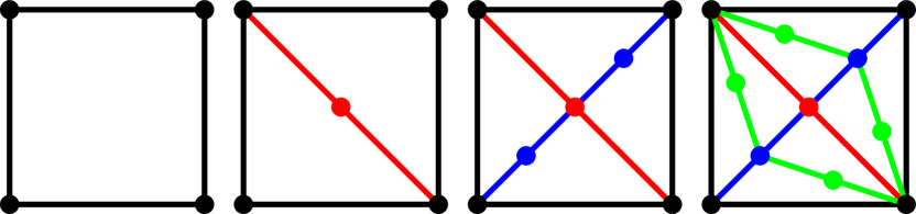
(a)

(b)

Figure 1.1. An example of an acylindrical subdivision rule on the top, and a cylindrical subdivision rule on the bottom.

1.2. Moduli space, finite approximation and renormalization

Our first result gives a precise description of the moduli space of subdivision graphs for $\mathcal{R}$. We remark that the techniques we use can be applied to more general subdivision rules. To simplify the presentation, we state our theorems for finite subdivision rules, and refer the readers to §7 for many generalizations.

Theorem A.

Let $\mathcal{R}$ be a simple, irreducible finite subdivision rule, consisting of polygons $\{P_{1},...,P_{k}\}$. Let $\mathcal{G}_{1},...,\mathcal{G}_{k}$ be the subdivision graphs for $\mathcal{R}$.

1. The subdivision graphs $\mathcal{G}_{i}$ are isomorphic to the nerves of infinite circle packings if and only if $\mathcal{R}$ is acylindrical;

2. Suppose that $\mathcal{R}$ is acylindrical. Then

   1. any two circle packings $\mathcal{P},\mathcal{P}^{\prime}$ with nerve $\mathcal{G}_{i}$ are quasiconformally homeomorphic, i.e., there exists a quasiconformal map $\Psi:\widehat{\mathbb{C}}\longrightarrow\widehat{\mathbb{C}}$ so that $\Psi(\Lambda(\mathcal{P}_{i}))=\Lambda(\mathcal{P}_{i}^{\prime})$;

   2. the moduli space $\mathcal{M}(\mathcal{G}_{i})$ is isometrically homeomorphic to the Teichmüller space $\operatorname{Teich}(\Pi_{F_{i}})$ of the ideal polygon associated to the external face of $F_{i}$.

Remark.

We remark that by (a), there is a natural Teichmüller metric on $\mathcal{M}(\mathcal{G}_{i})$, which is the metric used in (b). We also note that if $F_{i}$ has $e_{i}$ edges, then $\operatorname{Teich}(\Pi_{F_{i}})$ is homeomorphic to $\mathbb{R}^{e_{i}-3}$. Thus, the circle packing with nerve $\mathcal{G}_{i}$ is rigid if and only if $e_{i}=3$.

Exponential convergence of finite approximation

Let $\mathcal{P},\mathcal{P}^{\prime}\in\mathcal{M}(\mathcal{G}^{n}_{i})$. We say they have the same external class if $\pi_{F_{i}}(\mathcal{P})=\pi_{F_{i}}(\mathcal{P}^{\prime})$, where

$$\pi_{F_{i}}:\mathcal{M}(\mathcal{G}^{n}_{i})=\prod_{F\text{ face of }\mathcal{G}^{n}_{i}}\operatorname{Teich}(\Pi_{F})\longrightarrow\operatorname{Teich}(\Pi_{F_{i}})$$

is the projection map to the Teichmüller space for the external face $F_{i}$.

Suppose $\mathcal{R}$ is acylindrical. Theorem A implies that there exists a unique infinite circle packing for each external class. The existence and uniqueness are intimately connected. The infinite circle packing is constructed as the limit of finite circle packings for $\mathcal{G}^{n}_{i}$ with fixed external class. To put our rigidity result in perspective, note that a circle packing for $\mathcal{G}^{n}_{i}$ with a fixed external class is not rigid unless all non-external faces of $\mathcal{G}^{n}_{i}$ are triangles. Our second result shows that these finite circle packings stabilize exponentially fast (see Figure 1.2, c.f. [He91] and §1.5.2).

Theorem B.

Let $\mathcal{R}$ be a simple, irreducible, acylindrical finite subdivision rule, consisting of polygons $\{P_{1},...,P_{k}\}$. Let $\mathcal{G}_{1},...,\mathcal{G}_{k}$ be subdivision graphs for $\mathcal{R}$. Then there exist constants $C$, $n_{0}\in\mathbb{N}$ and $\delta<1$ so that for any $j$, the following holds.

Let $\mathcal{P},\mathcal{Q}$ be two finite circle packings for $\mathcal{G}_{i}^{n+j}$ with the same external class, where $n\geq n_{0}$. Let $\mathcal{P}^{j},\mathcal{Q}^{j}$ be the corresponding sub-circle packings associated to the subgraph $\mathcal{G}^{j}_{i}\subseteq\mathcal{G}^{n+j}_{i}$. Then

$$d(\mathcal{P}^{j},\mathcal{Q}^{j})\leq\min\{C,d(\mathcal{P},\mathcal{Q})\}\cdot\delta^{n-n_{0}},$$

where $d$ is the Teichmüller distance between the two circle packings.

This means that there exists a quasiconformal homeomorphism $\Psi:\hat{\mathbb{C}}\longrightarrow\hat{\mathbb{C}}$ between $\mathcal{P}^{j}$ and $\mathcal{Q}^{j}$ whose dilatation $K(\Psi)$ satisfying

$$\frac{1}{2}\log K(\Psi)\leq\min\{C,d(\mathcal{P},\mathcal{Q})\}\cdot\delta^{n-n_{0}}.$$

In particular, if we normalize the circle packings by Möbius transformations appropriately so that $\Psi$ fixes $0,1,\infty$, then

$$\|\Psi-id\|_{C^{0}}=O(\delta^{n}),$$

where $\|-\|_{C^{0}}$ is the $C^{0}$ norm with respect to the spherical metric.

Figure 1.2. The finite circle packings of level $0,1,2,3,4,15$ of the subdivision graph in Figure 1(a). These circle packings are chosen so that one can fit in a circle touching all four sides of each complementary quadrilateral region. One notices that the circles at a given level stabilize quite rapidly as asserted by Theorem B.

Renormalizations on circle packings

Let $\mathcal{P}$ be a circle packing with nerve $\mathcal{G}_{i}$. The complement of the union of ‘outermost’ closed disks consists of two regions. One of the two, denoted by $\Pi(\mathcal{P})$, has non-trivial intersection with the limit set $\Lambda(\mathcal{P})$. Define the space

$$\Sigma:=\bigcup_{i=1}^{k}\{(\mathcal{P},x):\mathcal{P}\in\mathcal{M}(\mathcal{G}_{i}),x\in\overline{\Pi(\mathcal{P})}\}/\operatorname{PSL}_{2}(\mathbb{C}).$$

By Theorem A, $\Sigma$ is homeomorphic to $\bigcup_{i=1}^{k}\mathbb{R}^{e_{i}-3}\times\overline{\Pi(\mathcal{P}_{i})}$, where $\mathcal{P}_{i}$ is (any) circle packing with nerve $\mathcal{G}_{i}$. Moreover, any two pairs $(\mathcal{P},x)$ and $(\mathcal{P}^{\prime},x^{\prime})$ on the same fiber are quasiconformally homeomorphic.

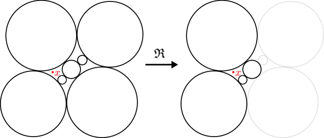
Figure 1.3. An illustration of the renormalization operator.

Let $\mathcal{Q}_{F}$ be the sub-circle packings of $\mathcal{P}$ corresponding to a face $F$ of $\mathcal{R}(P)$, and let $\Pi(\mathcal{Q}_{F})$ be the corresponding domain. Suppose that $x\in\overline{\Pi(\mathcal{Q}_{F})}\subseteq\overline{\Pi(\mathcal{P})}$. Then we define the renormalization of $(\mathcal{P},x)$ by

$$\mathfrak{R}((\mathcal{P},x))=(\mathcal{Q}_{F},x)\in\Sigma.$$

We remark that technically, if $x\in\partial\overline{\Pi(\mathcal{Q}_{F})}\cap\partial\overline{\Pi(\mathcal{Q}_{F^{\prime}})}$, then the definition of $\mathfrak{R}$ requires a choice. This happens if the point $x$ is the tangent point where two circles touch. We can resolve this issue by blowing up every tangent point into two points, and denote this new space by $\widetilde{\Sigma}$ with the projection map $\pi:\widetilde{\Sigma}\longrightarrow\Sigma$. In this way, we construct a renormalization operator

$$\mathfrak{R}:\widetilde{\Sigma}^{1}\subseteq\widetilde{\Sigma}\longrightarrow\widetilde{\Sigma}.$$

We say $(\mathcal{P},x)$ is infinitely renormalizable if $\mathfrak{R}^{n}$ is defined at $\pi^{-1}((\mathcal{P},x))$ for all $n$. It is easy to see that $(\mathcal{P},x)$ is infinitely renormalizable if and only if $x\in\Lambda(\mathcal{P})\cap\overline{\Pi(\mathcal{P})}$. Thus, the non-escaping locus $\widetilde{\Sigma}^{\infty}$ is homeomorphic to a fibration over a Cantor set, whose fibers are Euclidean spaces. It projects via $\pi$ to $\Sigma^{\infty}$, which is homeomorphic to $\bigcup_{i=1}^{k}\mathbb{R}^{e_{i}-3}\times(\Lambda(\mathcal{P}_{i})\cap\overline{\Pi(\mathcal{P}_{i})}).$

The following theorem states that as we zoom in at a limit point, a homeomorphism between two circle packings for subdivision graphs converges exponentially fast to a conformal map.

Theorem C.

Let $\mathcal{R}$ be a simple, irreducible, acylindrical finite subdivision rule, consisting of polygons $\{P_{1},...,P_{k}\}$. Let $\mathcal{G}_{i}$ be the subdivision graphs for $\mathcal{R}$. Then there exist constants $C$, $n_{0}\in\mathbb{N}$ and $\delta<1$ so that the following holds.

Suppose that $(\mathcal{P},x),(\mathcal{P}^{\prime},x^{\prime})\in\Sigma^{\infty}$ are homeomorphic. Then for all $n\geq n_{0}$,

$$d(\mathfrak{R}^{n}((\mathcal{P},x)),\mathfrak{R}^{n}((\mathcal{P}^{\prime},x^{\prime}))\leq\min\{C,d((\mathcal{P},x),(\mathcal{P}^{\prime},x^{\prime}))\}\cdot\delta^{n-n_{0}},$$

where $d$ is the Teichmüller metric.

We remark that $\mathfrak{R}^{n}((\mathcal{P},x))$ is interpreted as $\pi(\mathfrak{R}^{n}(\pi^{-1}((\mathcal{P},x))))$. In the case when $\pi^{-1}((\mathcal{P},x))$ consists of two points,

$$\mathfrak{R}^{n}((\mathcal{P},x))=\{(\mathcal{P}_{1,n},x_{1,n}),(\mathcal{P}_{2,n},x_{2,n})\}$$

consists of two points for all sufficiently large $n$. The Teichmüller distance is naturally defined on pairs of circle packings.

Universality and regularity

Once the exponential convergence of the renormalization is established, we can derive a number of consequences regarding the local geometry and universality of such circle packings (cf. [McM96, §9.4]).

Let $X\subseteq\widehat{\mathbb{C}}$ be a subset that is not necessarily open. A map $\Psi:X\longrightarrow\widehat{\mathbb{C}}$ is $C^{1+\alpha}$-conformal at $z$ if the complex derivative

$$\Psi^{\prime}(z):=\lim_{z+t\in X,t\to 0}\frac{\Psi(z+t)-\Psi(z)}{t}$$

exists, and

$$\Psi(z+t)=\Psi(z)+\Psi^{\prime}(z)t+O(|t|^{1+\alpha})$$

for all $z+t\in X$ and $t$ sufficiently small (cf. [McM96, §B.6]).

Theorem D.

Let $\mathcal{R}$ be a simple, irreducible, acylindrical finite subdivision rule, consisting of polygons $\{P_{1},...,P_{k}\}$. Let $\mathcal{G}_{i}$, $i=1,..,k$ be the subdivision graphs for $\mathcal{R}$.

1. Let $\mathcal{P},\mathcal{P}^{\prime}$ be two circle packings with nerve $\mathcal{G}_{i}$ and $\Psi$ be any homeomorphism between them. Then $\Psi|_{\Lambda(\mathcal{P})\cap\overline{\Pi(\mathcal{P})}}$ is $C^{1+\alpha}$-conformal.

2. Let $(\mathcal{P}_{0},x_{0})\in\Sigma^{\infty}$ be a renormalization periodic point with period $q$. Then there exists a Möbius map $\phi\in\operatorname{PSL}_{2}(\mathbb{C})$ so that $\phi((\Lambda(\mathcal{P}_{q}),x_{0}))=(\Lambda(\mathcal{P}_{0}),x_{0})$ where $\mathcal{P}_{q}$ is the subpacking of $\mathcal{P}_{0}$ corresponding to $\mathfrak{R}^{q}(\mathcal{P}_{0},x_{0})$. The multiplier $\mu:=\phi^{\prime}(x_{0})$ is called the scaling factor for $(\mathcal{P}_{0},x_{0})$.

3. Either

   • $x_{0}$ is a cusp point of $\partial\overline{\Pi(\mathcal{P}_{0})}$, in which case $\phi$ is a parabolic Möbius map with a fixed point at $x_{0}$; or

   • $x_{0}$ is not a cusp point of $\partial\overline{\Pi(\mathcal{P}_{0})}$, in which case the scaling factor satisfies $|\mu|>1$.

4. The scaling factor is universal, in the following sense. Let $\mathcal{Q}$ be an arbitrary circle packing. Suppose there exists a homeomorphism $\Psi:\widehat{\mathbb{C}}\longrightarrow\widehat{\mathbb{C}}$ so that $\Psi(\Lambda(\mathcal{P}_{0}))\subseteq\Lambda(\mathcal{Q})$. Then

   • $\Lambda(\mathcal{Q})$ is asympototically self-similar at $\Psi(x_{0})$ by a parabolic Möbius map if $|\mu|=1$.

   • $\Lambda(\mathcal{Q})$ is asympototically self-similar at $\Psi(x_{0})$ with scaling factor $\mu$ if $|\mu|>1$;

Remark.

We remark that there are few restrictions for the homeomorphism $\Psi$ on the interior of the disks for the circle packing. Thus the asymptotic conformality only applies to the restriction of $\Psi$ on the limit set.

In §5.5, we introduce the notion of a Teichmüller mapping between two circle packings, which is a homeomorphism between the circle packings that satisfies some additional desired properties. We proved that a Teichmüller mapping is asymptotically conformal at all combinatorially deep points (see Theorem 6.9 and Remark 6.10).

We also remark that since the scaling factor is $1$ at a cusp point of $\partial\overline{\Pi(\mathcal{P}_{0})}$, the renormalization operator $\mathfrak{R}$ is not a hyperbolic operator on $\Sigma^{\infty}$.

1.3. Existence and rigidity for spherical subdivision graphs

Subdivision graphs for a finite subdivision rule $\mathcal{R}$ has a special external face that is not subdivided. For many applications in dynamics and geometry, the circle packing is dense on the whole Riemann sphere. Such circle packings can be modeled by spherical subdivision graphs as follows.

$\mathcal{R}$-complexes

Let $\mathcal{R}$ be a finite subdivision rule. An $\mathcal{R}$-complex is a finite CW complex $X$ so that for any closed 2-cell $s$, there exist $P_{\sigma(s)}\in\{P_{i}:i=1,...,k\}$ and a cellular map $\psi_{s}:P_{\sigma(s)}\longrightarrow s$ that is a homeomorphism between the open 2-cells.

The subdivision rule gives a sequence of subdivisions $\mathcal{R}^{n}(X)$ for $X$. We always assume that $\mathcal{R}$ is the minimal finite subdivision rule that supports $X$, i.e. every polygon in $\{P_{i}:i=1,...,k\}$ appears as the type of some closed 2-cell of $\mathcal{R}^{n}(X)$ for some $n$. The 1-skeleton of subdivisions $\mathcal{R}^{n}(X)$ of $X$ gives a nested sequences of graphs

$$\mathcal{G}^{0}\subseteq\mathcal{G}^{1}\subseteq\mathcal{G}^{2}\subseteq...,\text{ and }\mathcal{G}=\lim_{\rightarrow}\mathcal{G}^{n}=\bigcup_{n}\mathcal{G}^{n}.$$

If the $\mathcal{R}$-complex $X$ is homeomorphic to a sphere, the plane graph $\mathcal{G}$ is called a spherical subdivision graph for $\mathcal{R}$. We remark that any spherical subdivision graph for $\mathcal{R}$ can be constructed by piecing together finitely many subdivision graphs of $\mathcal{R}$ along their boundaries.

Our next result gives a characterization of existence and rigidity.

Theorem E.

Let $\mathcal{G}$ be a simple spherical subdivision graph for an irreducible finite subdivision rule $\mathcal{R}$.

1. The graph $\mathcal{G}$ is isomorphic to the nerve of an infinite circle packing $\mathcal{P}$ if and only if $\mathcal{R}$ is acylindrical.

2. Moreover, if the circle packing exists, it is combinatorially rigid, i.e., there exists a unique circle packing up to Möbius maps with nerve $\mathcal{G}$.

Similar to the case of subdivision graphs, finite approximations stabilize exponentially fast.

Theorem F.

Let $\mathcal{G}$ be a simple spherical subdivision graph for an irreducible, acylindrical finite subdivision rule $\mathcal{R}$. Then there exist constants $C$, $n_{0}\in\mathbb{N}$ and $\delta<1$ so that for any $k$, the following holds.

Let $\mathcal{P},\mathcal{Q}$ be two circle packings for $\mathcal{G}^{n+k}$ where $n\geq n_{0}$. Let $\mathcal{P}^{k},\mathcal{Q}^{k}$ be the corresponding sub-circle packings for the subgraph $\mathcal{G}^{k}$. Then

$$d(\mathcal{P}^{k},\mathcal{Q}^{k})\leq C\delta^{n-n_{0}}.$$

1.4. Rigidity of Kleinian circle packings

A circle packing $\mathcal{P}$ is called Kleinian if its limit set $\Lambda(\mathcal{P})$ is equal to the limit set $\Lambda(\Gamma)$ of some Kleinian group $\Gamma$. The nerve of a Kleinian circle packing may not be a spherical subdivision graph for a finite subdivision rule, but instead follows a more general subdivision rule (see §7 and §8). In fact, the nerve of a geometrically finite Kleinian circle packing is a graph with finite subdivision rule if and only if the Kleinian group has no rank 2 cusps. Our theory is well-suited for this broader context. As an application, we prove the following.

Theorem G.

Let $\mathcal{P}$ be a Kleinian circle packing. Suppose the corresponding Kleinian group $\Gamma$ is geometrically finite. Then $\mathcal{P}$ is combinatorially rigid.

Remark.

We remark that geometrically infinite Kleinian circle packings are in general not combinatorially rigid. Indeed, by changing the ending lamination associated to the geometrically infinite end carefully, it is possible to change the limit set while the nerve for the circle packing remains constant.

1.5. Discussion on related work

1.5.1. Rigidity of hexagonal circle packing and other triangulations

Circle packings provide a conformally natural way to embed a planar graph into a surface. In the 1980s, Thurston proposed a constructive, geometric approach to the Riemann mapping theorem using circle packings. This conjecture was proved by Rodin-Sullivan in [RS87]. The proof depends crucially on the non-trivial uniqueness of the hexagonal packing as the only packing in the plane with nerve the triangular lattice.

Using combinatorial arguments, Schramm gave a generalization of the above rigidity result. Let $\mathcal{P}$ be a circle packing on the Riemann sphere $\widehat{\mathbb{C}}$ whose nerve $\mathcal{G}$ is a planar triangulation. In [Sch91, Theorem 1.1], Schramm proved that if $\widehat{\mathbb{C}}-\text{carrier}(\mathcal{P})$ is at most countable, then $\mathcal{P}$ is combinatorially rigid. Here the carrier of a packing $\mathcal{P}$ is the union of the closed disks in $\mathcal{P}$ and the ‘interstices’ bounded by three mutually touching circles in the complement of the packing. The rigidity of the hexagonal packing follows immediately, since the carrier is the whole complex plane.

He and Schramm continued to develop many new tools to weaken the hypothesis of above result. In [HS93], they proved a rigidity result with the hypothesis that $\widehat{\mathbb{C}}-\text{carrier}(\mathcal{P})$ is a countable union of points or disks. In [HS94], they proved a rigidity result for $\mathcal{P}$ with possibly uncountably many one-point components in $\widehat{\mathbb{C}}-\text{carrier}(\mathcal{P})$, but under the hypothesis that the boundary has $\sigma$-finite linear measure. These rigidity results have a close connection to the Koebe’s conjecture that every planar domain can be mapped conformally onto a circle domain, and the techniques in [HS93, HS94] led to a breakthrough towards the Koebe’s conjecture.

The concept of circle packings can be generalized to any closed orientable surface with a projective structure. A version of the Koebe-Andreev-Thurston theorem in this setting already appeared in [Thu82]. Since a surface of genus $g\geq 1$ in general supports many different projective structures, a natural question is to determine the subspace of projective structures supporting a circle packing with a fixed nerve. See [KMT03, KMT06] for results in this direction.

In the above mentioned work, the methods require crucially that the nerve is a triangulation. We remark that in our setting, the graph $\mathcal{G}$ is never a planar triangulation, nor locally finite.

1.5.2. Rate of convergence of finite circle packings

In his thesis [He91], He provided a quantitative estimate for the rate of convergence of finite approximation of the hexagonal circle packings. Let $\mathcal{G}$ be the nerve of the regular hexagonal circle packing. Then we have a natural level structure $\mathcal{G}^{0}\subseteq\mathcal{G}^{1}\subseteq\mathcal{G}^{2}\subseteq...$ where $\mathcal{G}^{0}$ is a single point, and $\mathcal{G}^{n}$ is the subgraph generated by $\mathcal{G}^{n-1}$ and all vertices adjacent to $\mathcal{G}^{n-1}$. Let $\mathcal{P}^{n},\mathcal{Q}^{n}$ be two circle packing of $\mathbb{C}$ with nerve $\mathcal{G}^{n}$. Let $\mathcal{P}^{1},\mathcal{Q}^{1}$ be the subpackings corresponding to the subgraph $\mathcal{G}^{1}\subseteq\mathcal{G}^{n}$. Then with appropriate normalization, He proved that there exists a homeomorphism $\Psi:\mathbb{C}\longrightarrow\mathbb{C}$ that sends the circle packing $\mathcal{P}^{1}$ to $\mathcal{Q}^{1}$ with $\|\Psi-id\|_{C^{0}}=O(\frac{1}{n})$ (cf. exponential convergence in Theorem B and F). This estimate gives a quantitative bound on the convergence of the discrete Riemann mapping in [RS87]. See also [HR93, HS96, HS98, HL10] for some generalizations, which are closely related to regularity of local symmetries.

1.5.3. Finite subdivision rules

With a motivation from the Cannon’s conjecture, finite subdivision rules are introduced and studied extensively in a series of papers by Cannon, Floyd and Parry [CFP01, CFP06a, CFP06b]. They appear naturally in the study of dynamics of rational maps and geometric group theory (see [CFKP03, CFP07, CFPP09]). Some connections between finite subdivision rules and circle packings have been explored in [BS97, Ste03, BS17].

In those previous work mentioned above, it is usually assumed that the the subdivision has bounded valence and it satisfies some expansion property, such as mesh approaching zero (see [CFP06a, CFP06b]). This expansion property requires that the edges are cut into smaller and smaller pieces for iterations of the subdivision. This is in contrast with the setting of this paper. The subdivision we obtain always have infinite valence. Moreover, in order to create an infinite graph from the 1-skeleton, the mesh is never shrinking to zero (see Assumption (2) in Definition 1.2).

1.5.4. Quasisymmetric rigidity

A Schottky set is the complement of a union of disjoint open disks in $\widehat{\mathbb{C}}$. This includes examples like circle packings and round Sierpinski carpets. In [BKM09], it is proved that a Schottky set $X$ with zero area is quasisymmetrically rigid. More precisely, any quasisymmetric homeomorphism of $X$ is the restriction of a Möbius map. Also see [BM13] for other quasisymmetric rigidity results. We remark that it is crucial that the homeomorphisms are quasisymmetric in this general setting as any two Sierpinski carpets are homeomorphic.

Quasisymmetric symmetries of relative Schottky sets are studied in [Mer12, Mer14]. We remark that a Schottky set has a different definition in [Mer12, Mer14] compared to [BKM09]. In order to apply He-Schramm’s uniformization results for relative circle domains, and with the main application on quasisymmetry groups of a Sierpiski carpet Julia set in mind, it is assumed in [Mer12, Mer14] that the complementary disks of a Schottky set have disjoint closures. In particular, it does not cover the case that we are considering in this paper. It is proved that the any local quasisymmetric symmetry has complex derivative on the Schottky set (see [Mer12, Theorem 1.2]), and the derivative is bi-Lipschitz (see [Mer12, Proposition 8.2]) (cf. Theorem D). It is conjectured that a local quasisymmetric symmetry possesses higher degree of regularity (see [Mer12, Conjecture 1.3]).

An immediate consequence of quasisymmetric rigidity for a fractal set is the identification of its quasisymmetric and conformal symmetry groups. In our context, the homeomorphism group of the limit set of a circle packing whose nerve is a spherical subdivision graph for a finite subdivision rule can already be identified with the conformal symmetry group, generalizing the result for Apollonian gaskets in [LLMM23].

1.5.5. Kleinian circle packings

Let $\Gamma$ be a geometrically finite Kleinian group whose limit set $\Lambda(\Gamma)$ is equal to the limit set $\Lambda(\mathcal{P})$ of an infinite circle packing $\mathcal{P}$. Then the corresponding three manifold $M=\Gamma\backslash\mathbb{H}^{3}$ is acylindrical (cf. Theorem 8.1). For acylindrical Kleinian group, it follows from [McM90] that there exists a unique Kleinian group with totally geodesic boundary in its quasiconformal conjugacy class. Such Kleinian groups have Schottky sets as their limit sets, and provide many examples of Kleinian circle packings.

The Apollonian circle packing is an example of a Kleinian circle packing, and its arithmetic, geometric, and dynamical properties have been extensively studied in the literature (for a non-exhaustive list, see e.g. [GLMWY03, GLMWY05, BF11, KO11, OS12, BK14, Zha22]). More recently, there have been many new and exciting developments in the study of more general Kleinian circle packings [KN19, KK21, BKK22, LLM22].

1.5.6. Renormalization and iterations on Teichmüller spaces

Renormalization was introduced into dynamics in the mid 1970s by Feigenbaum, Coullet and Tresser, and it has established itself as a powerful tool for the study of nonlinear systems whose essential form is repeated at infinitely many scales (for a non-exhaustive list, see e.g. [DH85, McM94, McM96, McM98, Lyu99, IS08, AL11, DLS20, AL22]). The connections between renormalization theories of quadratic polynomials and Kleinian groups are explained in [McM96]. Iterations on Teichmüller spaces have many applications in dynamics and geometry (see e.g. [Thu88, McM90, DH93, Sel11]).

1.5.7. Further applications

It is conjectured that besides some trivial examples, the Julia set of a rational map is not quasiconformally homeomorphic to the limit set of a Kleinian group (see [LLMM23]). This conjecture is proved in various settings when the Julia set or the limit set is a Sierpinski carpet (see [BLM16, QYZ19]). In an upcoming sequel [LZ23], the rigidity results in this paper will be used to prove the conjecture for circle packing limit sets of reflection groups.

In an upcoming paper of the first author and D. Ntalampekos, the exponential contraction of renormalizations will play an important role in characterizing Julia sets that can be quasiconformally uniformized to a circle packing (c.f. [Bon11, BLM16] for Sierpinski carpet Julia sets, and [McM90] for Sierpinski carpet/circle packing limit sets).

1.6. Methods and outline

In §2, we recall some classical results on the moduli spaces of finite circle packings, and relate these moduli spaces to Teichmüller spaces.

The skinning map for circle packings is introduced in §3. Roughly speaking, let $\mathcal{H}$ be a subgraph of a finite graph $\mathcal{G}$. The natural pullback of the inclusion map $i:\mathcal{H}\longrightarrow\mathcal{G}$ gives a map on the moduli space

$$\tau=\tau_{\mathcal{H},\mathcal{G}}:\mathcal{M}(\mathcal{G})\longrightarrow\mathcal{M}(\mathcal{H}).$$

We then characterize when the image $\tau(\mathcal{M}(\mathcal{G}))$ is bounded in $\mathcal{M}(\mathcal{H})$ based on how $\mathcal{H}$ sits in $\mathcal{G}$ (see Theorem 3.2 and 3.3). The construction and the theorems are motivated by Thurston’s Bounded Image Theorem for skinning maps of hyperbolic 3-manifolds (see the discussion in §3.1).

The Bounded Image Theorem provides compactness. In §4, we prove the existence part of Theorem A and E by taking geometric limit.

The skinning map we constructed is the restriction on some real slice of a holomorphic map between Teichmüller spaces. Thus it is a contraction with respect to the Teichmüller metric. Toegether with the Bounded Image Theorem, the contraction is uniform. In §5, we apply iterations of the skinning map to harvest compounding contraction. This allows us to prove uniqueness, and more generally, the exponential convergence results.

In §6, we apply these exponential convergence results to prove the regularity and universality results. With the appropriate setup, the argument is similar as in the renormalization theory.

Finally, in §7, we illustrate how our methods can be generalized to other subdivision rules. In particular, we consider the case of interpolations of finite subdivision rules (see Theorem 7.4) as well as $\mathbb{Z}^{2}$-subdivision rule (see Theorem 7.7). The former allows us to change the combinatorics of circle packings, and lays down the foundations to study parameter spaces of circle packings in the future. The latter provides a model for rank 2 cusps in a Kleinian group, which is used in §8 to show geometrically finite Kleinian circle packings are combinatorially rigid.

Acknowledgement

The authors thank Seigei Merenkov for explaining to us the literature and his work on rigidity results for circle packings, along with many invaluable suggestions. The authors also thank Dima Dudko, Misha Lyubich and Curt McMullen for many useful discussions. The circle packings in Figure 1.2 are produced with the program GOPack developed by C. Collins, G. Orick and K. Stephenson [COK17]. The limit sets in Figures 6.1, 7.2 and 8.5 are produced with C. McMullen’s program lim.

2. Teichmüller space and finite circle packings

In this section, we recall some facts about finite circle packings and their deformation spaces. Many details can be found in [LLM22]; see also [Bro85, Bro86].

Let $\mathcal{G}$ be a connected finite simple plane graph, and let $\mathcal{P}$ be any finite circle packing whose nerve is isomorphic to $\mathcal{G}$, as guaranteed by the Finite Circle Packing Theorem. The disks in $\mathcal{P}$ are marked by the vertices of the graph $\mathcal{G}$, and we denote the open round disk corresponding to a vertex $v$ by $D_{v,\mathcal{P}}$, and its boundary circle by $C_{v,\mathcal{P}}$. Define the Moduli space of marked finite circle packings associated to $\mathcal{G}$ as follows:

$$\begin{split}\mathcal{M}(\mathcal{G}):=\{\mathcal{P}\text{ is a marked finite }&\text{circle packing}\\ &\text{whose nerve is isomorphic to $\mathcal{G}$}\}/\sim\end{split}$$

where $\mathcal{P}^{\prime}\sim\mathcal{P}$ if there exists a Möbius transformation $\eta$ so that $D_{v,\mathcal{P}^{\prime}}=\eta(D_{v,\mathcal{P}})$ for every vertex $v$ of $\mathcal{G}$. A natural topology on the space is defined by $\mathcal{P}_{i}\to\mathcal{P}$ if $D_{v,\mathcal{P}_{i}}\to D_{v,\mathcal{P}}$ for every vertex $v$.

From now on, generally for simplicity, we drop the dependence on $\mathcal{P}$ in the notations when it is clear which packing we refer to. Given $\mathcal{P}\in\mathcal{M}(\mathcal{G})$, let $\Gamma$ be the group generated by reflections in the circles $C_{v}$. This group is called the kissing reflection group associated to $\mathcal{P}$ in [LLM22].

Let $\operatorname{Aut}^{\pm}(\hat{\mathbb{C}})\cong\operatorname{Isom}(\mathbb{H}^{3})$ be the group of Möbius and anti-Möbius transformations, which is also the group of isometries of $\mathbb{H}^{3}$. A quasiconformal deformation of $\Gamma$ is a discrete and faithful representation $\xi:\Gamma\longrightarrow\operatorname{Aut}^{\pm}(\hat{\mathbb{C}})$ that preserves parabolics, induced by a quasiconformal map $f:\hat{\mathbb{C}}\longrightarrow\hat{\mathbb{C}}$ (i.e. $\xi(\gamma)=f\circ\gamma\circ f^{-1}$ for all $\gamma\in\Gamma$).

The quasiconformal deformation space of $\Gamma$ is defined as

$$\mathcal{QC}(\Gamma):=\{\xi:\Gamma\longrightarrow\operatorname{Aut}^{\pm}(\hat{\mathbb{C}})\text{ is a quasiconformal deformation}\}/\sim$$

where $\xi\sim\xi^{\prime}$ if they are conjugates of each other by a Möbius transformation. We can put the algebraic topology on the space, i.e. $\xi_{i}\to\xi$ if $\xi_{i}(\gamma)\to\xi(\gamma)$ for all $\gamma\in\Gamma$.

The discussion in [LLM22] implies the following identification:

Proposition 2.1.

For any connected finite simple plane graph $\mathcal{G}$,

$$\mathcal{M}(\mathcal{G})\cong\mathcal{QC}(\Gamma).$$

Let $F$ be a face of $\mathcal{G}$. Then there exists a polygon $P_{F}$ and a cellular map $\psi_{F}:P_{F}\longrightarrow F$ which restricts to a homeomorphism between the interiors. Note that the map $\psi_{F}$ is a homeomorphism if and only if $F$ is a Jordan domain. The boundary $\partial P_{F}$ is called the ideal boundary of $F$, and is denoted by $I(F)$. Abusing notations, we often use the same symbols to denote vertices and edges of $P_{F}$ and those of $F$, especially when $F$ is a Jordan domain.

Consider the following set

$$\Pi:=\hat{\mathbb{C}}-\bigcup_{v}\overline{D_{v}}.$$

Each face $F$ of $\mathcal{G}$ gives a connected component $\Pi_{F}$ of $\Pi$, which we call the interstice of the packing $\mathcal{P}$ for the face $F$. Note that $\Pi_{F}$ is the interior of an ideal polygon with the same number of vertices as $I(F)$.

The group $\Gamma$ contains a subgroup of index $2$ of orientation preserving elements, which we denote by $\widetilde{\Gamma}$. Let $\Lambda$ and $\Omega$ be its limit set and domain of discontinuity respectively. Note that $\Pi_{F}$ is contained in a unique component $\Omega_{F}$ of $\Omega$. Let $\Gamma_{F}$ be the subgroup of $\Gamma$ generated by circles corresponding to vertices of $F$. Then $\Pi_{F}$ is the interior of a fundamental domain of the action of $\Gamma_{F}$ on $\Omega_{F}$.

It is easy to see that $\widetilde{\Gamma}$ is geometrically finite, i.e. its action on the hyperbolic 3-space $\mathbb{H}^{3}$ has a finite-sided fundamental polyhedron. Consider the Kleinian manifold

$$M:=\widetilde{\Gamma}\backslash(\mathbb{H}^{3}\cup\Omega).$$

Its boundary $\partial M=\bigcup_{F}X_{F}$ has a connected component for each face $F$ of $\mathcal{G}$. Each $X_{F}$ is topologically a punctured sphere, and its number of punctures is the same as the number of vertices of $F$. Conformally, $X_{F}\cong\widetilde{\Gamma}_{F}\backslash\Omega_{F}$, where $\widetilde{\Gamma}_{F}$ is the index 2 subgroup of $\Gamma_{F}$ consisting of orientation preserving elements. In fact, it is conformally the double of $\Pi_{F}$. The anti-holomorphic reflection that exchanges the two copies of $\Pi_{F}$ is an involution, denoted by $\sigma_{F}:X_{F}\longrightarrow X_{F}$.

By the quasiconformal deformation theory of Ahlfors, Bers, Maskit and others, including a nicely presented version of Sullivan [Sul81], there exists a holomorphic surjection

$$\Psi:\prod_{F}\operatorname{Teich}(X_{F})\longrightarrow\mathcal{QC}(\widetilde{\Gamma}),$$

which is a homeomorphism if each component of $\Omega$ is simply connected. The failure of injectivity comes from a component of $\Omega$ that is not simply connected, e.g. by performing a Dehn twist along an essential curve in that component which is homotopically trivial in the three manifold $M$. This map restricts to a surjection

$$\Psi:\prod_{F}\operatorname{Teich}^{\sigma_{F}}(X_{F})\longrightarrow\mathcal{QC}(\Gamma),$$

where $\operatorname{Teich}^{\sigma_{F}}(X_{F})$ denotes the quasiconformal deformation space of $X_{F}$ invariant under $\sigma_{F}$. Note that since $X_{F}$ is determined by $\Pi_{F}$, we also view $\operatorname{Teich}^{\sigma_{F}}(X_{F})\cong\operatorname{Teich}(\Pi_{F})$ as a deformation space of the ideal polygon $\Pi_{F}$.

We claim this restriction is also injective. Indeed, non-injectivity is only possible if there exist two different ways of decomposing some $X_{F}$ into two equal pieces of ideal polygon, together with an anti-holomorphic involution that exchanges the two pieces. Conformally, we can put one piece in the upper half plane, and the other piece the lower half plane, with punctures on the extended real line. It is then clear that the only anti-holomorphic involution is $z\mapsto\bar{z}$.

Combined with Proposition 2.1, we have

Theorem 2.2.

For any connected finite simple plane graph $\mathcal{G}$,

$$\mathcal{M}(\mathcal{G})\cong\prod_{F}\operatorname{Teich}(\Pi_{F}).$$

Moreover, it is easy to see that the identification above is isometric with respect to the Teichmüller metric on $\mathcal{QC}(\Gamma)$ and that of the product $\prod_{F}\operatorname{Teich}(\Pi_{F})$, defined as the maximum of the Teichmüller metrics on $\operatorname{Teich}(\Pi_{F})$.

Fenchel-Nielsen coordinates

Given a face $F$ with the cellular map $\psi_{F}:P_{F}\longrightarrow F$, any pair of non-adjacent vertices $v,w$ of $I(F)$ gives rise to an essential simple closed curve $\widetilde{\gamma}^{F}_{vw}$ of $X_{F}$, invariant under the involution $\sigma_{F}$.

More precisely, if $\psi_{F}(v)\neq\psi_{F}(w)$, let $g_{v}$ and $g_{w}$ be the reflections in the circles $C_{v}$ and $C_{w}$ respectively (note that here we use the same symbols to denote the corresponding vertices of $F$). Then the element $g_{v}g_{w}\in\widetilde{\Gamma}_{F}$ is loxodromic and determines the curve $\widetilde{\gamma}^{F}_{vw}$ on $X_{F}$. On the other hand, if $\psi_{F}(v)=\psi_{F}(w)$, then this curve can be represented by a nontrivial loop in $\Omega_{F}$, but is null-homotopic in $M$, so cannot be represented by a nontrivial element in $\widetilde{\Gamma}$ (for an illuminating picture, see [LLM22, Fig. 3.1]).

Geometrically, note that $v,w$ determine two non-adjacent sides $I_{v}$ and $I_{w}$ of the interstice $\Pi_{F}$. In the hyperbolic metric induced from $X_{F}$, let $\gamma^{F}_{vw}$ be the geodesic segment perpendicular to both $I_{v}$ and $I_{w}$. The double of $\gamma^{F}_{vw}$ in $X_{F}$ is the simple closed geodesic $\widetilde{\gamma}^{F}_{vw}$. We remark that every $\sigma_{F}$-invariant simple closed geodesic on $X_{F}$ arises this way.

Note that we can decompose $X_{F}$ into pairs of pants along a maximal collection of disjoint $\sigma_{F}$-invariant simple closed geodesics. Indeed, any such decomposition comes from a triangulation of $F$, where added edges between two non-adjacent vertices of $F$ determine the collection of simple closed geodesics in the way described above. The hyperbolic structure on $X_{F}$ is completely determined by the hyperbolic lengths of geodesics in this collection. This gives Fenchel-Nielsen coordinates on

$$\operatorname{Teich}(\Pi_{F})\cong\operatorname{Teich}^{\sigma_{F}}(X_{F})\cong\mathbb{R}_{+}^{m-3}$$

where $m$ is the number of vertices of $F$. Note that there are no twist parameters due to $\sigma_{F}$-invariance.

Finally, we remark that to go to infinity in $\operatorname{Teich}(\Pi_{F})$, some geodesic arc $\gamma_{vw}^{F}$ must shrink to zero. Given $\epsilon>0$, define $\operatorname{Teich}_{\geq\epsilon}(\Pi_{F})\subseteq\operatorname{Teich}(\Pi_{F})$ to be the subset of ideal polygons satisfying the condition that for any non-adjacent pair of vertices $v,w$, the geodesic arc $\gamma_{vw}^{F}$ has hyperbolic length $\geq\epsilon$.

Proposition 2.3.

For any $\epsilon>0$, $\operatorname{Teich}_{\geq\epsilon}(\Pi_{F})$ is compact.

Proof.

Note that in $\operatorname{Teich}_{\geq\epsilon}(\Pi_{F})$, given a pair of non-adjacent vertices $v,w$, for any point $x$ on $\gamma_{vw}^{F}$, on one of the two sides, a perpendicular geodesic segment starting at $x$ of length $\epsilon/2$ is contained entirely in $\Pi_{F}$. Since the hyperbolic area of $\Pi_{F}$ is fixed, this gives an upper bound on the length of $\gamma_{vw}^{F}$ as well. ∎

3. The skinning map and bounded image theorem

In this section, we will define the skinning map for circle packings, and characterize when a skinning map has bounded image.

Let $\mathcal{G}$ be a connected finite simple plane graph and $\mathcal{H}\subseteq\mathcal{G}$ be a connected induced subgraph, i.e., a connected graph formed by a subset of the vertices of $\mathcal{G}$ and all of the edges connecting pairs of vertices in the subset.

Then there exists a natural pullback of the inclusion map $i:\mathcal{H}\xhookrightarrow{}\mathcal{G}$ on the moduli space

$$\tau=\tau_{\mathcal{H},\mathcal{G}}:\mathcal{M}(\mathcal{G})\longrightarrow\mathcal{M}(\mathcal{H}).$$

Indeed, if $\mathcal{P}\in\mathcal{M}(\mathcal{G})$ is a circle packing with nerve $\mathcal{G}$, and $\mathcal{Q}$ be the corresponding sub-circle packing associated to $\mathcal{H}$, then $\tau(\mathcal{P})=\mathcal{Q}$. We call this map $\tau$ the skinning map associated to $\mathcal{H}\subseteq\mathcal{G}$.

We now define an important notion of cylindrical and acylindrical subgraphs (cf. Definition 1.3 and Figure 1.1).

Definition 3.1.

Let $F$ be a face of $\mathcal{H}$ that is a Jordan domain. It is called acylindrical in $\mathcal{G}$ if for any two non-adjacent vertices $v,w\in\partial F$, the two components of $\partial F-\{v,w\}$ are connected in $F\cap\mathcal{G}-\{v,w\}$. Otherwise, it is called cylindrical in $\mathcal{G}$.

Suppose all faces of $\mathcal{H}$ are Jordan domains. The subgraph $\mathcal{H}$ is called acylindrical in $\mathcal{G}$ if every face of $\mathcal{H}$ is acylindrical in $\mathcal{G}$. Otherwise, it is called acylindrical in $\mathcal{G}$.

The following is the analogue of Thurston’s Bounded Image Theorem in our setting (see [Thu82]).

Theorem 3.2 (Bounded Image Theorem).

Let $\mathcal{G}$ be a connected finite simple plane graph, and $\mathcal{H}\subseteq\mathcal{G}$ be a connected induced subgraph. Suppose that every face of $\mathcal{H}$ is a Jordan domain. Then the image $\tau(\mathcal{M}(\mathcal{G}))\subseteq\mathcal{M}(\mathcal{H})$ is bounded if and only if $\mathcal{H}$ is acylindrical in $\mathcal{G}$.

Recall that by Theorem 2.2, we have

$$\mathcal{M}(\mathcal{H})=\prod_{F\text{ face of }\mathcal{H}}\operatorname{Teich}(\Pi_{F}).$$

Let $\pi_{F}:\mathcal{M}(\mathcal{H})\longrightarrow\operatorname{Teich}(\Pi_{F})$ be the corresponding projection. We actually prove the following stronger version of the Bounded Image Theorem.

Theorem 3.3 (Relative Bounded Image Theorem).

Let $\mathcal{G}$ be a connected finite simple plane graph, and $\mathcal{H}\subseteq\mathcal{G}$ be a connected induced subgraph. Let $F$ be a face of $\mathcal{H}$ that is a Jordan domain. Then the image $\pi_{F}(\tau(\mathcal{M}(\mathcal{G})))\subseteq\operatorname{Teich}(\Pi_{F})$ is bounded if and only if $F$ is acylindrical in $\mathcal{G}$.

3.1. Topological descriptions

In this subsection, we give a topological description of acylindricity, and compare the skinning maps for circle packings with Thurston’s skinning maps. The aim is to provide motivation and connect our combinatorially definition to many well-known concepts in hyperbolic geometry and topology. Our proof of the Bounded Image Theorem is self-contained and does not require this connection.

Compressing disks

Let $\mathcal{P}$ be a circle packing with nerve $\mathcal{H}$. As in §2, let $\Gamma$ be the group generated by reflections along circles in $\mathcal{P}$, and $\widetilde{\Gamma}$ be the index 2 subgroup of $\Gamma$. Let $F$ be a face of $\mathcal{H}$. Then $F$ corresponds to a boundary component $X_{F}$ of the Kleinian manifold $M=\widetilde{\Gamma}\backslash(\mathbb{H}^{3}\cup\Omega(\widetilde{\Gamma}))$.

A compressing disk $D$ is an embedded disk in $M$ with $\partial D\subseteq\partial M$. It is a non-trivial if $\partial D$ does not bound a disk in $\partial M$. We say a component $X_{F}\subseteq\partial M$ is incompressible if every compressing disk $D$ with $\partial D\subseteq X_{F}$ is trivial.

The following gives a topological characterization for Jordan domain faces.

Theorem 3.4.

Let $F$ be a face of $\mathcal{H}$. Then $F$ is a Jordan domain if and only if $X_{F}$ is incompressible.

Proof.

It is easy to see that $X_{F}$ is incompressible if and only if the corresponding domain of discontinuity $\Omega_{F}$ is simply connected. This is equivalent to the fact that the limit set $\Lambda_{F}$ of the group $\Gamma_{F}$ is connected.

On the other hand, $\partial F$ is not 2-connected precisely when $F$ is not a Jordan domain, as deleting any repeated vertex separates the graph. The theorem then follows from [LLM22, Prop. 3.4]. ∎

Cylinders

Let $F$ be a face of $\mathcal{H}\subseteq\mathcal{G}$ that is a Jordan domain. Let $\mathcal{P}_{F}$ be a finite circle packing with nerve $F\cap\mathcal{G}$. Denote the corresponding reflection group, Kleinian group and Kleinian manifold by $\Gamma_{F}$, $\widetilde{\Gamma}_{F}$ and $M_{F}$.

Let $F_{ext}$ be the external face of $F\cap\mathcal{G}$, i.e., $F_{ext}=\overline{\widehat{\mathbb{C}}-F}$. Let $X_{ext}\subseteq\partial M_{F}$ be the corresponding surface.

A cylinder is a continuous map

$$f:(S^{1}\times[0,1],S^{1}\times\{0,1\})\longrightarrow(M_{F},\partial M_{F}).$$

It is called essential if its boundary components $f(S^{1}\times\{0\}),f(S^{1}\times\{1\})$ are essential curves of $\partial M_{F}$. A cylinder is boundary parallel if it can be homotoped rel boundary to a cylinder in $\partial M_{F}$.

The following theorem provides an equivalent topological definition of acylindrical faces in $\mathcal{G}$.

Theorem 3.5.

Let $F$ be a face of $\mathcal{H}\subseteq\mathcal{G}$ that is a Jordan domain. Then $F$ is acylindrical in $\mathcal{G}$ if and only if every cylinder with one boundary component in $X_{ext}$ is boundary parallel.

Proof.

Suppose $F$ is cylindrical in $\mathcal{G}$. Then there exists two non-adjacent vertices $v,w$ on $\partial F$, and a face $F^{\prime}$ of $\mathcal{G}$ so that $v,w\in F^{\prime}$. Let $g_{v}$ and $g_{w}$ be reflections in $C_{v}$ and $C_{w}$ respectively. Then $g_{v}g_{w}$ is in both $\widetilde{\Gamma}_{F^{\prime}}$ and $\widetilde{\Gamma}_{F_{ext}}$. In other words, the curves $\tilde{\gamma}_{vw}^{F^{\prime}}$ and $\tilde{\gamma}_{vw}^{F_{ext}}$ are homotopic in $M_{F}$. The homotopy between them gives an essential cylinder that is not boundary parallel.

Conversely, suppose $f:(S^{1}\times[0,1],S^{1}\times\{0,1\})\longrightarrow(\mathcal{M}_{F},\partial\mathcal{M}_{F})$ is an essential cylinder with $f(S^{1}\times\{0\})\subset X_{ext}$ and $f(S^{1}\times\{0\})\subset X_{F^{\prime}}$ for some face $F^{\prime}$ of $\mathcal{G}$. Assume further the cylinder is not boundary parallel. Then there exists a lift of $f$

$$\tilde{f}:\mathbb{R}\times[0,1]\longrightarrow\mathbb{H}^{3}\cup\Omega_{F}$$

so that $\tilde{f}(\mathbb{R}\times\{0\})\subset\Omega_{ext}$ and $\tilde{f}(\mathbb{R}\times\{0\})\subset g\cdot\Omega_{F^{\prime}}$ for some $g\in\Gamma_{F}$. Moreover we may assume the two endpoints of $f(\mathbb{R}\times\{0\})$ lie in two different circles $C_{v}$ and $C_{w}$ for a pair of non-adjacent $v,w\in\partial F$. Since the endpoints of $f(\mathbb{R}\times\{1\})$ are the same as those of $f(\mathbb{R}\times\{0\})$, we conclude that for some $g^{\prime}$ in the stabilizer of $\Omega_{F}^{\prime}$ in $\Gamma_{F}$, $gg^{\prime}\cdot\Pi_{F^{\prime}}$ must be bounded by arcs on $C_{v}$ and $C_{w}$. This immediately imply that $gg^{\prime}\cdot\Pi_{F^{\prime}}=\Pi_{F^{\prime}}$, as any further reflections are contained in one of the circles in $\mathcal{P}_{F}$, and thus cannot intersect two. Hence $v,w\in F^{\prime}$ and we conclude that $F$ is cylindrical. ∎

Skinning maps

Let $\Gamma$ be a geometrically finite Kleinian group, with Kleinian manifold $M$. Suppose $\partial M$ is incompressible. Then the quasiconformal deformation space of $\Gamma$ can be identified with $\operatorname{Teich}(\partial M)$. The cover of $\operatorname{Int}(M)$ corresponding to $\partial M$ is a finite union of quasi-Fuchsian manifolds, and we obtain a map

$$\operatorname{Teich}(\partial M)\longrightarrow\operatorname{Teich}(\partial M)\times\operatorname{Teich}(\overline{\partial M}).$$

The first coordinate is the identity map, and the second coordinate is Thurston’s skinning map

$$\tau_{M}:\operatorname{Teich}(\partial M)\longrightarrow\operatorname{Teich}(\overline{\partial M}),$$

which reveals the surface obscured by the topology of $M$ (see [Ken10]).

To see the connection with our setting, let us consider the following situation. Let $\mathcal{G}$ be a finite simple plane graph. Suppose that the faces $F_{1},...,F_{k}$ of $\mathcal{G}$ are all Jordan domains. Let $\mathcal{H}_{i}=\partial F_{i}$.

Let $\mathcal{P}$ be a circle packing with nerve $\mathcal{G}$, and $\Gamma$ be the group generated by reflection along circles in $\mathcal{P}$. Let $M$ be the Kleinian manifold for the index 2 subgroup of $\Gamma$ with the reflection map $\sigma:M\longrightarrow M$. We denote by $\Gamma_{i}$ and $M_{i}$ the subgroup and Kleinian manifold associated to $\mathcal{H}_{i}$. Note that each $M_{i}$ is a quasi-Fuchsian manifold. Then by Theorem 2.2, we have

$$\mathcal{M}(\mathcal{G})=\operatorname{Teich}^{\sigma}(\partial M)\text{ and }\mathcal{M}(\mathcal{H}_{i})=\operatorname{Teich}^{\sigma}(\partial M_{i}).$$

Note that

$$\operatorname{Teich}(\partial M)\times\operatorname{Teich}(\overline{\partial M})=\prod_{i}\operatorname{Teich}(\partial M_{i}).$$

Putting everything together, we have the following theorem giving a precise connection of Thurston’s skinning map and the skinning maps in our setting.

Theorem 3.6.

With the notations above, Thurston’s skinning map

$$(id,\tau_{M}):\operatorname{Teich}(\partial M)\longrightarrow\operatorname{Teich}(\partial M)\times\operatorname{Teich}(\overline{\partial M})=\prod_{i}\operatorname{Teich}(\partial M_{i})$$

restricts to a map

$$(id,\tau_{M}):\operatorname{Teich}^{\sigma}(\partial M)=\mathcal{M}(\mathcal{G})\longrightarrow\operatorname{Teich}^{\sigma}(\partial M)\times\operatorname{Teich}^{\sigma}(\overline{\partial M})=\prod_{i}\mathcal{M}(\mathcal{H}_{i}).$$

Moreover, we have the identity $(id,\tau_{M})|_{\operatorname{Teich}^{\sigma}(\partial M)}=\prod_{i}\tau_{\mathcal{H}_{i},\mathcal{G}}$

Proof.

For each face $F_{i}$ of $\mathcal{G}$, the stabilizer of the corresponding domain of discontinuity $\Omega_{i}$ is precisely $\Gamma_{i}$. So the restriction of the Thurston’s skinning map to the reflection locus has image in the reflection locus. Since $\Gamma_{i}$ comes from the reflection group generated by circles corresponding to vertices in $\mathcal{H}_{i}$, it follows that this restriction manifests as the product of $\tau_{\mathcal{H}_{i},\mathcal{G}}$ for circle packings. ∎

3.2. Well-connectedness

In this subsection, we prove the following proposition which says acylindrical subgraphs contains a lot of connecting paths.

Proposition 3.7.

Let $F$ be a face of $\mathcal{H}\subseteq\mathcal{G}$ that is a Jordan domain. Suppose that $F$ is acylindrical in $\mathcal{G}$. Then for any pair of non-adjacent vertices $v,w\in\partial F$, there exists a simple path $\gamma\in F\cap\mathcal{G}$ connecting $v,w$ so that $\operatorname{Int}(\gamma)\subseteq\operatorname{Int}(F)$.

To prove this, we first state the following separation lemma.

Lemma 3.8.

Let $F$ be a face of $\mathcal{H}\subseteq\mathcal{G}$ that is a Jordan domain. Suppose that $F$ is acylindrical in $\mathcal{G}$. Then for any pair of non-adjacent vertices $x,y\in\partial F$, there exists a path $\alpha\in F\cap\mathcal{G}$ with $\operatorname{Int}(\alpha)\subseteq\operatorname{Int}(F)$ that separates $x,y$ in $F$. More precisely, $x,y$ are in two different components of $F-\alpha$.

Proof.

Since $F$ is acylindrical in $\mathcal{G}$, there exists a path $\alpha\in F\cap\mathcal{G}$ that connects the two components of $\partial F-\{x,y\}$. This path $\alpha$ separates $x,y$. ∎

Proof of Proposition 3.7.

First note that since we can construct a simple path from a path by deleting closed loops, it suffices to construct a path $\gamma\in F\cap\mathcal{G}$ connecting $v,w$ so that $\operatorname{Int}(\gamma)\subseteq\operatorname{Int}(F)$.

To construct this path, we first pick the two adjacent vertices $x_{1},y_{1}\in\partial F$ of $v$, and let $I_{1}$ be the component of $\partial F-\{x_{1},y_{1}\}$ that contains $w$. By Lemma 3.8, there exists a path $\gamma_{1}$ connecting $v$ to $v_{1}$ where $v_{1}\in I_{1}$ with $\operatorname{Int}(\gamma_{1})\subseteq\operatorname{Int}(F)$.

Let $I_{2}$ be the component of $\partial F-\{v,v_{1}\}$ that contains $w$. Clearly, the two boundary points in $\partial I_{2}$ are non-adjacent. Now applying Lemma 3.8 to the two points in $\partial I_{2}$ and obtain a path $\gamma_{2}$ connecting a point $v_{2}\in I_{2}$ to $\partial F-\overline{I_{2}}$. Since the end points of $\gamma_{1}$ and $\gamma_{2}$ are linked, $\operatorname{Int}(\gamma_{1})\cup\operatorname{Int}(\gamma_{2})$ is connected.

Inductively, suppose $w\notin\{v,v_{1},v_{2},...,v_{k-1}\}$. Then let $I_{k}$ be the component of $\partial F-\{v,v_{1},v_{2},...,v_{k-1}\}$ that contains $w$. We can apply Lemma 3.8 to $\partial I_{k}$ and obtain a path $\gamma_{k}$ connecting $v_{k}\in I_{k}$ to $\partial F-\overline{I_{k}}$ with $\operatorname{Int}(\gamma_{k})\subseteq\operatorname{Int}(F)$. By construction, it is easy to see that $\operatorname{Int}(\gamma_{1})\cup...\cup\operatorname{Int}(\gamma_{k})$ is connected.

Since the number of vertices in $I_{k}$ by at least $1$ less than the number of vertices in $I_{k-1}$, this process eventually terminates, say at $k$. Thus, $w=v_{k}$ is an end point of $\gamma_{k}$. Since $\operatorname{Int}(\gamma_{1})\cup...\cup\operatorname{Int}(\gamma_{k})$ is connected, we can find a path connecting $v,w$ as desired. ∎

3.3. Bounded image theorem

In this subsection, we prove Theorem 3.3, from which Theorem 3.2 follows immediately. We remark that it is possible to give a similar argument as in Thurston’s original proof of the Bounded Image Theorem [Thu82].

Proof of Theorem 3.3.

Suppose that $F$ is cylindrical. Then there exist non-adjacent vertices $v,w\in\partial F$, and a face $F^{\prime}$ of $\mathcal{G}$ contained in $F$ so that $v,w\in F^{\prime}$. Let $\Gamma_{\mathcal{G}}$ be the reflection groups associated to a circle packing $\mathcal{P}_{\mathcal{G}}$ with nerve $\mathcal{G}$. Similarly, let $\Gamma_{\mathcal{H}}\subseteq\Gamma_{\mathcal{G}}$ be the subgroup associated to the induced subgraph $\mathcal{H}$.

As in §2, let $\Omega_{F^{\prime}}$ (and $\Omega_{F}$) be the component of domain of discontinuity for $\Gamma_{\mathcal{G}}$ (and $\Gamma_{\mathcal{H}}$) associated to $F^{\prime}$ (and $F$ respectively). Note that $\Omega_{F^{\prime}}\subseteq\Omega_{F}$. We also denote by $\Gamma_{F}$, $\Gamma_{F^{\prime}}$ the groups generated by circles corresponding to vertices of $F$, $F^{\prime}$ respectively, and $\widetilde{\Gamma}_{F}$, $\widetilde{\Gamma}_{F^{\prime}}$ their index 2 subgroups of orientation preserving elements. Let $g_{v},g_{w}\in\Gamma_{\mathcal{H}}\subseteq\Gamma_{\mathcal{G}}$ be reflections along circles $C_{v},C_{w}$ respectively. Then $g_{v},g_{w}\in\Gamma_{F}\cap\Gamma_{F^{\prime}})$. Since $v,w$ are non-adjacent in $\partial F$ and $\mathcal{H}$ is an induced subgraph of $\mathcal{G}$, they are non-adjacent in the ideal boundary $I(F^{\prime})$ of $F^{\prime}$. Thus, the product $g_{v}g_{w}$ corresponds to $\sigma$-invariant simple closed curves $\gamma$ and $\gamma^{\prime}$ in $X_{F}:=\widetilde{\Gamma}_{F}\backslash\Omega_{F}$ and $X_{F^{\prime}}:=\widetilde{\Gamma}_{F^{\prime}}\backslash\Omega_{F^{\prime}}$. Since $\Omega_{F^{\prime}}\subseteq\Omega_{F}$, we have the length satisfies

$$l_{X_{F}}(\gamma)\leq l_{X_{F^{\prime}}}(\gamma^{\prime}).$$

By quasiconformally deforming the surface $X_{F^{\prime}}$, we can find a sequence in $\mathcal{M}(\mathcal{G})$ so that the length of $\gamma^{\prime}$ is shrinking to $0$. By the above inequality, the length of $\gamma$ is also shrinking to $0$. Thus, the image of this sequence under

$$\pi_{F}\circ\tau:\mathcal{M}(\mathcal{G})\longrightarrow\operatorname{Teich}(\Pi_{F})$$

is not bounded. This proves one direction.

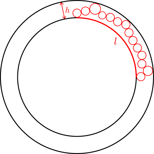
Figure 3.1. A bound on the modulus.

Conversely, suppose that $F$ is acylindrical. Let $\mathcal{P}_{\mathcal{G}}$ be a circle packing with nerve $\mathcal{G}$ and $\mathcal{P}_{\mathcal{H}}$ be the sub-circle packing associated to $\mathcal{H}$.

Let $\Pi_{F}$ be the interstice of the circle packing $\mathcal{P}_{\mathcal{H}}$ for the face $F$, i.e., the interior of the fundamental domain associated to $F$. Note that $\Pi_{F}$ is bounded by circular arcs from circles of $\mathcal{P}_{\mathcal{H}}$ associated to $\partial F$. Let $v,w$ be two non-adjacent vertices on $\partial F$, and let $I_{v},I_{w}$ be the two corresponding circular arcs on $\partial\Pi_{F}$. Then we obtain a quadrilateral $(\overline{\Pi_{F}},I_{v}\cup I_{w})$, which is conformally equivalent to

$$([0,t]\times[0,1],[0,t]\times\{0,1\}).$$

Here $t=\operatorname{Mod}((\overline{\Pi_{F}},I_{v}\cup I_{w}))$ is the conformal modulus of $(\overline{\Pi_{F}},I_{v}\cup I_{w})$.

Let us normalize by a Möbius map so that $C_{v}$ and $C_{w}$ are circles centered at $0$ with radius $1$ and $R>1$. Since $F$ is acylindrical, there exists a finite chain of circles in the closed annulus $\overline{A(R)}=\overline{B(0,R)}-B(0,1)$ that bounds the arc $I_{v}$ (see Figure 3.1). Let $l$ be the length of the arc $I_{v}$ and $h=R-1$, then $l/h$ is bounded above by the number of circles in this chain. Hence, $\operatorname{Mod}(A(R))=\frac{\log(R)}{2\pi}$ is bounded away from $0$. Therefore, $\operatorname{Mod}((\overline{\Pi_{F}},I_{v}\cup I_{w}))\leq\frac{1}{\operatorname{Mod}(A(R))}$ is bounded from above. Let $\gamma_{vw}$ be the simple closed curve on $X_{F}$ associated to the non-adjacent pair $(v,w)$. Then there exists a lower bound for the hyperbolic length $l_{X_{F}}(\gamma_{vw})$. Since this holds for any pair of non-adjacent vertices on $\partial F$, the image $\pi_{F}(\tau(\mathcal{M}(\mathcal{G})))$ is bounded in $\operatorname{Teich}(\Pi_{F})$ by Proposition 2.3. ∎

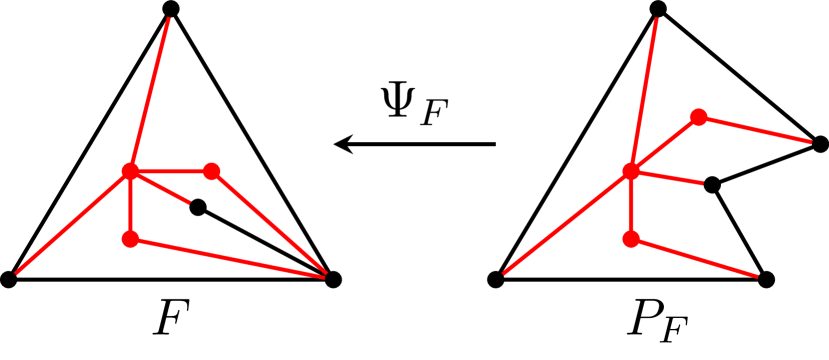
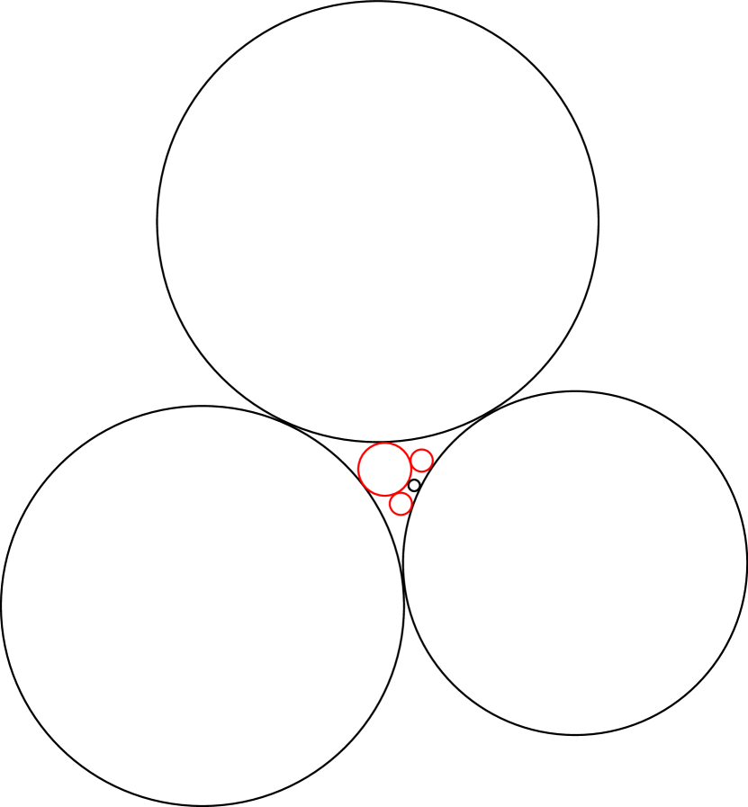
Figure 3.2. A counterexample with non-Jordan domains.

3.4. A counterexample with non-Jordan domains

We end our discussion with a counterexample showing that the Jordan domain assumption in the Bounded Image Theorem is essential.

Consider the example as Figure 3.2. The graph $\mathcal{H}$ is in black, and the graph $\mathcal{G}$ is the union of black and red edges. The bounded face $F$ of $\mathcal{H}$ is not a Jordan domain. Let $\Psi_{F}:P_{F}\longrightarrow F$ be the cellular map which restricts to a homeomorphism in the interior. Note that $P_{F}$ is acylindrical to the pullback of the graph $\mathcal{G}$. A circle packing with nerve $\mathcal{G}$ is depicted in the bottom of Figure 3.2. It is easy to see that we can shrink the small black circle to a point while fixing the other three black circles in $\mathcal{M}(\mathcal{G})$. Therefore, $\pi_{F}\circ\tau(\mathcal{M}(\mathcal{G}))$ is not bounded in $\operatorname{Teich}(\Pi_{F})$.

4. Existence of circle packings

The Bounded Image Theorem (Theorem 3.2) provides precompactness for finite circle packings, and allow us to take limit. In this section, we will prove the existence part of Theorem A and Theorem E.

Theorem 4.1.

Let $\mathcal{R}$ be an irreducible simple finite subdivision rule, with subdivision graphs $\mathcal{G}_{i},i=1,...,k$. Let $\mathcal{G}$ be a simple spherical subdivision graph for $\mathcal{R}$.

• The subdivision graphs $\mathcal{G}_{i}$ are isomorphic to the nerves of infinite circle packings $\mathcal{P}_{i}$ if and only if $\mathcal{R}$ is acylindrical.

• The spherical subdivision graph $\mathcal{G}$ is isomorphic to the nerve of an infinite circle packing $\mathcal{P}$ if and only if $\mathcal{R}$ is acylindrical.

4.1. Subdivision with Jordan domain faces

To apply the Bounded Image Theorem, we will need to construct a modification of $\mathcal{R}$ so that all the faces of the subdivision are Jordan domains.

Let $\mathcal{R}$ be an irreducible simple finite subdivision rule, consisting of polygons $\{P_{1},...,P_{k}\}$. Suppose that $\mathcal{R}$ is acylindrical.

Recall that $\mathcal{G}^{n}_{i}$ is the 1-skeleton of $\mathcal{R}^{n}(P_{i})$. Note that there exists a unique face of $\mathcal{G}^{n}_{i}$ that is not contained in $P_{i}$, which we will call the external face. Otherwise, it is a non-external face.

Since $\mathcal{R}$ is irreducible, $\mathcal{G}^{n}_{i}$ is an induced subgraph of $\mathcal{G}^{n+1}_{i}$. Since $\mathcal{R}$ is acylindrical, by replacing $\mathcal{R}$ with an iterate if necessary, we assume that

• the face $P_{i}$ of $\mathcal{G}^{0}_{i}$ is acylindrical in $\mathcal{G}^{1}_{i}$.

Lemma 4.2.

For each $i$, there exist graphs $\widetilde{\mathcal{G}}^{1}_{i}$ with

$$\mathcal{G}^{1}_{i}\subseteq\widetilde{\mathcal{G}}^{1}_{i}\subseteq\mathcal{G}^{2}_{i}$$

so that every face of $\widetilde{\mathcal{G}}^{1}_{i}$ is a Jordan domain.

Proof.

Let $F$ be a non-external face of $\mathcal{G}^{1}_{i}$. Suppose that $F$ is not a Jordan domain. Let $\psi_{F}:P_{F}\longrightarrow F$ be the cellular map given by the subdivision rule, where $P_{F}\in\{P_{1},...,P_{k}\}$. We denote the pullback of $\mathcal{G}^{2}_{i}$ by $\psi_{F}^{*}(\mathcal{G}^{2}_{i})$. More precisely,

$$\psi_{F}^{*}(\mathcal{G}^{2}_{i}):=\psi_{F}^{-1}(F\cap\mathcal{G}^{2}_{i}).$$

Note that $P_{F}$ is acylindrical in $\psi_{F}^{*}(\mathcal{G}^{2}_{i})$. Therefore, by Proposition 3.7, for any pair of non-adjacent vertices $v,w\in\partial P_{F}$, there exists a simple path $\gamma$ in $\psi_{F}^{*}(\mathcal{G}^{2}_{i})$ with $\operatorname{Int}(\gamma)\subseteq\operatorname{Int}(P_{F})$ connecting $v,w$. By adding finitely many such paths $\gamma_{1},...,\gamma_{k}$, we can make sure that every face $F^{\prime}\subseteq F$ of $\partial F\cup\psi_{F}(\bigcup\gamma_{i})$ is a Jordan domain.

Let $\widetilde{\mathcal{G}}^{1}_{i}$ be the graph by adding all such paths in every non-Jordan domain face of $\mathcal{G}^{1}_{i}$. This graph $\widetilde{\mathcal{G}}^{1}_{i}$ satisfies the requirement. ∎

Now we can construct a new finite subdivision rule $\widetilde{\mathcal{R}}$. It contains polygons $\{P_{1},...,P_{k},Q_{1},...,Q_{l}\}$, where $P_{i}$ is the polygon in the original finite subdivision rule $\mathcal{R}$, and $Q_{1},...,Q_{l}$ are non-external faces of $\widetilde{\mathcal{G}}^{1}_{i}$ that are not faces of $\mathcal{G}^{1}_{i}$ where $i=1,..,k$.

For each polygon $P_{i}$, the subdivision $\widetilde{\mathcal{R}}(P_{i})$ is defined so that the 1-skeleton of $\widetilde{\mathcal{R}}(P_{i})$ is $\widetilde{\mathcal{G}}^{1}_{i}$. By construction, each face of $\widetilde{\mathcal{R}}(P_{i})$ can be identified with a polygon in $\{P_{1},...,P_{k},Q_{1},...,Q_{l}\}$, and each edge of $\partial P_{i}$ contains no vertices of $\widetilde{\mathcal{R}}(P_{i})$.

Now consider a polygon $Q_{j}$. By definition, we can identify $Q_{j}$ as a face of $\widetilde{\mathcal{G}}^{1}_{i}$ for some $i$. Since each face of $\mathcal{R}(P_{i})$ can be identified with a polygon in $\{P_{1},..,P_{k}\}$, we can consider the subdivision $\widetilde{\mathcal{R}}(\mathcal{R}(P_{i}))$. Then we have

$$P_{i}\preceq\mathcal{R}(P_{i})\preceq\widetilde{\mathcal{R}}(P_{i})\preceq\mathcal{R}^{2}(P_{i})\preceq\widetilde{\mathcal{R}}(\mathcal{R}(P_{i}))\preceq\mathcal{R}^{3}(P_{i})$$

where $A\preceq B$ means that $B$ is a subdivision of $A$. Equivalently, denote the 1-skeleton of $\widetilde{\mathcal{R}}(\mathcal{R}(P_{i}))$ by $\widetilde{\mathcal{G}}^{2}_{i}$. Then we have

$$\mathcal{G}^{1}_{i}\subseteq\widetilde{\mathcal{G}}^{1}_{i}\subseteq\mathcal{G}^{2}_{i}\subseteq\widetilde{\mathcal{G}}^{2}_{i}\subseteq\mathcal{G}^{3}_{i}.$$

Since $Q_{j}$ is a face of $\widetilde{\mathcal{G}}^{1}_{i}$, we define the subdivision $\widetilde{\mathcal{R}}(Q_{j})$ so that the 1-skeleton of $\widetilde{\mathcal{R}}(Q_{j})$ is $\widetilde{\mathcal{G}}^{2}_{i}\cap Q_{j}$. By construction, each face of $\widetilde{\mathcal{R}}(Q_{j})$ can be identified with a polygon in $\{P_{1},...,P_{k},Q_{1},...,Q_{l}\}$, and each edge of $\partial Q_{j}$ contains no vertices of $\widetilde{\mathcal{R}}(Q_{j})$.

In this way, we obtain a new finite subdivision rule $\widetilde{\mathcal{R}}$.

Proposition 4.3.

Let $\mathcal{R}$ be an irreducible simple finite subdivision rule, consisting of polygons $\{P_{1},...,P_{k}\}$. Suppose that $\mathcal{R}$ is acylindrical. Then by replacing $\mathcal{R}$ with an iterate if necessary, there exists an irreducible simple acylindrical finite subdivision rule $\widetilde{\mathcal{R}}$ consisting of polygons

$$\{P_{1},...,P_{k},Q_{1},...,Q_{l}\}$$

with the following properties.

1. The subdivisions satisfy

   $$\mathcal{R}^{n}(P_{i})\preceq\widetilde{\mathcal{R}}^{n}(P_{i})\preceq\mathcal{R}^{n+1}(P_{i});$$

   or equivalently, the 1-skeletons satisfy

   $$\mathcal{G}^{n}_{i}\subseteq\widetilde{\mathcal{G}}^{n}_{i}\subseteq\mathcal{G}^{n+1}_{i}$$

   for all $i=1,..,k$ and $n\geq 1$. In particular, $\mathcal{G}_{i}=\widetilde{\mathcal{G}}_{i}$ for all $i=1,..,k$.

2. Every face of $\widetilde{\mathcal{R}}^{n}(P_{i})$ or $\widetilde{\mathcal{R}}^{n}(Q_{j})$ is a Jordan domain for all $i=1,...,k,j=1,...,l$ and $n\geq 1$.

Proof.

It is clear that $\widetilde{\mathcal{R}}$ constructed above is simple, and acylindrical. By subdividing the polygons in $\{P_{1},...,P_{k},Q_{1},...,Q_{l}\}$, we can also make sure that $\widetilde{\mathcal{R}}$ is irreducible.

To prove $(1)$, we note that by construction, we have $\widetilde{\mathcal{R}}^{2}(P_{i})=\widetilde{\mathcal{R}}(\mathcal{R}(P_{i}))$ for all $i$. Since each face of $\mathcal{R}^{j}(P_{i})$ can be identified with one of the polygons in $\{P_{1},..,P_{k}\}$,

$$\widetilde{\mathcal{R}}(\mathcal{R}^{n-1}(P_{i}))=\widetilde{\mathcal{R}}(\mathcal{R}((\mathcal{R}^{n-2}(P_{i})))=\widetilde{\mathcal{R}}^{2}(\mathcal{R}^{n-2}(P_{i}))=...=\widetilde{\mathcal{R}}^{n}(P_{i}).$$

Let $F$ be a face of $\mathcal{R}^{n-1}(P_{i})$. Then $\mathcal{R}(F)\preceq\widetilde{\mathcal{R}}(F)\preceq\mathcal{R}^{2}(F)$. Therefore, we have $\mathcal{R}^{n}(P_{i})\preceq\widetilde{\mathcal{R}}^{n}(P_{i})=\widetilde{\mathcal{R}}(\mathcal{R}^{n-1}(P_{i}))\preceq\mathcal{R}^{n+1}(P_{i})$.

To prove $(2)$, it suffices to show that every face of $\widetilde{\mathcal{R}}(P_{i})$ and $\widetilde{\mathcal{R}}(Q_{j})$ is a Jordan domain. The statement is clear from our construction for $\widetilde{\mathcal{R}}(P_{i})$.

To prove the statement for $\widetilde{\mathcal{R}}(Q_{j})$, we first claim that every face of $\widetilde{\mathcal{R}}^{2}(P_{i})$ is a Jordan domain.

Proof of the claim.

Let $F$ be a face of $\widetilde{\mathcal{R}}^{2}(P_{i})=\widetilde{\mathcal{R}}(\mathcal{R}(P_{i}))$. Let $F^{\prime}$ be a face of $\mathcal{R}(P_{i})$ so that $F\subseteq F^{\prime}$. Let $\psi_{F^{\prime}}:P_{F^{\prime}}\longrightarrow F^{\prime}$ be the cellular map. Then by the construction of $\widetilde{\mathcal{R}}$, $\psi_{F^{\prime}}^{-1}(F)$ is a Jordan domain. Since that $P_{i}$ is acylindrical in $\mathcal{G}^{1}_{i}$ for all $i$, and $\mathcal{R}(F^{\prime})\preceq\widetilde{\mathcal{R}}(F^{\prime})$, we have that $\partial P_{F^{\prime}}$ is acylindrical in $\psi_{F^{\prime}}^{*}(\widetilde{\mathcal{G}}^{2}_{i})$. Therefore,

• either the face $\psi_{F^{\prime}}^{-1}(F)$ is disjoint from $\partial P_{F^{\prime}}$; or

• $\psi_{F^{\prime}}^{-1}(F)\cap\partial P_{F^{\prime}}$ is a single vertex; or

• $\psi_{F^{\prime}}^{-1}(F)\cap\partial P_{F^{\prime}}$ is a single edge.

In all three cases, we conclude that $F$ is also a Jordan domain. ∎

Since we can identify the polygon $Q_{j}$ with a face of $\widetilde{\mathcal{R}}(P_{i})$ and $\widetilde{\mathcal{R}}(Q_{j})=\widetilde{\mathcal{R}}^{2}(P_{i})\cap Q_{j}$, the statement for $\widetilde{\mathcal{R}}(Q_{j})$ follows immediately from the claim. ∎

A similar argument gives the following version for spherical subdivision graphs.

Proposition 4.4.

Let $\mathcal{G}$ be a simple spherical subdivision graph with irreducible finite subdivision rule $\mathcal{R}$. Suppose that $\mathcal{R}$ is acylindrical. Then by replacing $\mathcal{R}$ with another if necessary, we have that every face of $\mathcal{G}^{n}$ is a Jordan domain for all $n\geq 0$.

4.2. Cylindrical subdivisions

In this subsection, we shall prove the following characterization of cylindrical subdivisions.

Proposition 4.5.

Let $\mathcal{R}$ be a simple irreducible finite subdivision rule, consisting of polygons $\{P_{1},...,P_{k}\}$. Suppose that $\mathcal{R}$ is cylindrical. Then there exist a finite number $K$ and a pair of non-adjacent vertices $v,w\in\partial P_{i}$ so that there are infinitely many paths of length $\leq K$ in $\mathcal{G}_{i}$ connecting $v,w$ with pairwise disjoint interiors.

Proof.

Suppose that $\mathcal{R}$ is cylindrical. Then there exists a pair of $v,w\in\partial P_{i}$ so that $\partial P_{i}-\{v,w\}$ are in different components of $\mathcal{G}^{n}_{i}-\{v,w\}$ for all $n$. Therefore, there exists a face $F_{n}$ of $\mathcal{G}^{n}_{i}$ so that $v,w\in\partial F_{n}$. We may assume the faces are nested, i.e., $F_{n+1}\subseteq F_{n}$. Since the subdivision is non-trivial, i.e., $\mathcal{R}(P_{i})$ consists of at least two faces, $F_{n+1}$ is a proper subset of $F_{n}$. Let $\gamma_{n}\subseteq\partial F_{n}$ be a path connecting $v,w$. Since $F_{n}$ are all different, we may assume $\gamma_{n}$ are all different. Since $F_{n}$ is a face, the lengths of $\gamma_{n}$ are all bounded by some number $K$. We need to show we can choose them so that they have pairwise disjoint interiors.

Suppose for each $\gamma_{k}$, there are only finitely many $\gamma_{n}$ with $\operatorname{Int}(\gamma_{k})\cap\operatorname{Int}(\gamma_{n})\neq\emptyset$, then we can inductively select infinitely many paths $\gamma_{n_{k}}$ that satisfy the requirement of the proposition.

Thus, we may assume that there are infinitely many $\gamma_{n}$ with $\operatorname{Int}(\gamma_{k})\cap\operatorname{Int}(\gamma_{n})\neq\emptyset$. By the subdivision rule, we may assume $k=0$. Since the faces $F_{n}$ form a nested sequence, we may assume $\operatorname{Int}(\gamma_{0})\cap\operatorname{Int}(\gamma_{n})\neq\emptyset$ for all $n$. We can choose $v^{\prime},w^{\prime}\in\gamma_{0}$ so that $\{v^{\prime},w^{\prime}\}\neq\{v,w\}$ and $v^{\prime},w^{\prime}\in\gamma_{n}$ for all $n$. Denote by $\gamma^{\prime}_{n}$ the subpath of $\gamma_{n}$ that connects $v^{\prime},w^{\prime}$. Then $\gamma^{\prime}_{n}$ is a path in $F_{n}$ that connects $v^{\prime},w^{\prime}$, and the length of $\gamma^{\prime}_{n}$ is at most $K-1$. Since $\mathcal{R}$ is irreducible and simple and $F_{n}$ contains $v,w$ on its boundary, $v^{\prime},w^{\prime}$ are non-adjacent vertices in the ideal boundary of $F_{n}$ for all $n\geq 1$. Thus, by considering $\gamma^{\prime}_{n},n\geq 1$ as paths in $F_{1}$ if necessary, we may assume that $v^{\prime},w^{\prime}$ are non-adjacent vertices.

Thus, we obtain infinitely many different paths connecting two non-adjacent vertices with length $\leq K-1$. This process must terminate as the lengths of paths are positive integers. The proposition follows. ∎

4.3. Existence of circle packings

Proof of Theorem 4.1.

Let us prove the case for subdivision graphs. The statement for spherical subdivision graph can be proved in a similar way.

Suppose that $\mathcal{R}$ is acylindrical. Consider the sequence $\mathcal{G}^{n}_{i}$. By Proposition 4.3, we may assume that all faces of $\mathcal{G}^{n}_{i}$ are Jordan domains. Let $F_{ext}$ be the external face. By Theorem 2.2, we have

$$\mathcal{M}(\mathcal{G}^{n}_{i})=\prod_{F\text{ face of }\mathcal{G}^{n}_{i}}\operatorname{Teich}(\Pi_{F})=\prod_{F\text{ non-external}}\operatorname{Teich}(\Pi_{F})\times\operatorname{Teich}(\Pi_{F_{ext}}).$$

Fix a conformal structure $\sigma_{ext}\in\operatorname{Teich}(\Pi_{F_{ext}})$, and let $\mathcal{P}^{n}_{i}\in\mathcal{M}(\mathcal{G}^{n}_{i})$ be a circle packing with nerve $\mathcal{G}^{n}_{i}$ so that it has $\sigma_{ext}$ for $\operatorname{Teich}(\Pi_{F_{ext}})$.

Consider the sequence of circle packings $(\mathcal{P}^{n}_{i}:n\in\mathbb{N})$. Let $\tau_{k,n}:\mathcal{M}(\mathcal{G}^{n}_{i})\longrightarrow\mathcal{M}(\mathcal{G}^{k}_{i})$ be the skinning map, where $n>k$. By construction, we have

$$\pi_{F_{ext}}(\tau_{k,n}(\mathcal{P}^{n}_{i}))=\sigma_{ext}.$$

Let $F$ be a non-external face of $\mathcal{G}^{k}_{i}$. Then $F$ is acylindrical in $\mathcal{G}^{n}_{i}$ for all $n>k$. Therefore, by Theorem 3.3,

$$\pi_{F}(\tau_{k,n}(\mathcal{M}(\mathcal{G}^{n}_{i})))=\pi_{F}(\tau_{k,k+1}(\tau_{k+1,n}(\mathcal{M}(\mathcal{G}^{n}_{i}))))\subseteq\pi_{F}(\tau_{k,k+1}(\mathcal{M}(\mathcal{G}^{k+1}_{i})))$$

is uniformly bounded for all $n>k$. Combining the two, we conclude that

$$\{\tau_{k,n}(\mathcal{P}^{n}_{i}):n>k\}$$

is a bounded subset of $\mathcal{M}(\mathcal{G}^{k}_{i})$.

We assume the normalizations are chosen so that the level $0$ circle packings do not shrink to a point. By choosing a subsequence, we assume that $\Lambda(\mathcal{P}^{n}_{i})$ converges to a closed set in Gromov-Hausdorff topology. Since $\tau_{k,n}(\mathcal{P}^{n}_{i})$ is bounded in $\mathcal{M}(\mathcal{G}^{k}_{i})$,

$$\Lambda^{k}:=\lim_{n\to\infty}\Lambda(\tau_{k,n}(\mathcal{P}^{n}_{i}))$$

exists and is the limit set of a circle packing with nerve $\mathcal{G}^{n}_{i}$. Note that $\Lambda^{k}\subseteq\Lambda^{n}$ if $n\geq k$. Let $\Lambda^{\infty}=\overline{\bigcup_{k}\Lambda^{k}}$. Then $\Lambda^{\infty}$ is the limit set of an infinite circle packing with nerve $\mathcal{G}_{i}$.

Conversely, suppose that $\mathcal{R}$ is cylindrical. By Proposition 4.5, there exists a pair of non-adjacent vertices $v,w\in\partial P_{i}$ with infinitely many paths in $\mathcal{G}_{i}$ of uniformly bounded length connecting $v,w$ with pairwise disjoint interiors. Suppose for contradiction that $\mathcal{P}_{i}$ is a circle packing with nerve $\mathcal{G}_{i}$. The complement of the union of ‘outermost’ closed disks consists of two regions, and let $\Pi(\mathcal{P}_{i})$ be the component that has non-trivial intersection with the limit set $\Lambda(\mathcal{P}_{i})$. Let $I_{v},I_{w}$ be the circular arcs on $\partial\Pi(\mathcal{P}_{i})$ corresponding to the vertices $v,w$. Then the conformal modulus of the quadrilateral $(\overline{\Pi(\mathcal{P}_{i})},I_{v}\cup I_{w})$ is a finite number. However, there are infinitely many distinct chain of touching circles in $\overline{\Pi(\mathcal{P}_{i})}$ with bounded length that connects $I_{v}$ and $I_{w}$. This is impossible, and thus the theorem follows. ∎

Let $\mathcal{M}(\mathcal{G}_{i}):=\{\mathcal{P}_{i}:\mathcal{P}_{i}\text{ has nerve }\mathcal{G}_{i}\}/\operatorname{PSL}_{2}(\mathbb{C})$ be the moduli space with nerve $\mathcal{G}_{i}$. Let $F_{i}$ be the external face of $\mathcal{G}_{i}$. Then there exists a map

$$\Phi_{i}:\mathcal{M}(\mathcal{G}_{i})\longrightarrow\operatorname{Teich}(\Pi_{F_{i}}).$$

Note that the proof of Theorem 4.1 actually shows that

Proposition 4.6.

Suppose that $\mathcal{R}$ is acylindrical. Then $\Phi_{i}$ is surjective.

We will see in §5.3 that this map is a isometric bijection with respect to the Teichmüller metrics.

5. Iterations of the skinning map

Since the skinning map is a holomorphic map between Teichmüller spaces, it is a contraction with respect to the Teichmüller metric. By the Bounded Image Theorem, we have a uniform contraction. In this section, we make the above observations precise and iterate the skinning map to harvest compounding contraction. This allows us to prove exponential convergence of finite approximations as well as that of renormalizations. These results of exponential convergence then imply rigidity of circle packings.

5.1. The set up

Let $\mathcal{R}$ be a simple irreducible acylindrical finite subdivision rule, consisting of polygons $\{P_{1},...,P_{k}\}$. By Proposition 4.3 and replacing $\mathcal{R}$ with an appropriate one if necessary, we may assume that

1. every face $F$ of $\mathcal{G}_{i}^{k}$ is a Jordan domain; and

2. every non-external face $F$ of $\mathcal{G}_{i}^{k}$ is acylindrical in $\mathcal{G}_{i}^{n}$ for all $n>k$.

A finite list of maps $\tau_{F}$

Let $F$ be a face of $\mathcal{G}_{i}^{1}$, and let $\mathcal{H}_{F}=\partial F$ be the induced subgraph of $\mathcal{G}_{i}^{1}$. As $F$ is a Jordan domain, $\mathcal{H}_{F}$ has exactly two faces, one of which being $F$; denote by $F^{c}$ the other face. Thus, we have

$$\mathcal{M}(\mathcal{H}_{F})=\operatorname{Teich}(\Pi_{F})\times\operatorname{Teich}(\Pi_{F^{c}}).$$

We define the map

$$\tau_{F}:\mathcal{M}(\mathcal{G}_{i}^{1})=\prod_{S\text{ face of }\mathcal{G}_{i}^{1}}\operatorname{Teich}(\Pi_{S})\longrightarrow\operatorname{Teich}(\Pi_{F^{c}})$$

by $\tau_{F}(\mathcal{P})=\pi_{F^{c}}(\tau_{\mathcal{H}_{F},\mathcal{G}^{1}_{i}}(\mathcal{P}))$, where $\tau_{\mathcal{H}_{F},\mathcal{G}^{1}_{i}}:\mathcal{M}(\mathcal{G}_{i}^{1})\longrightarrow\mathcal{M}(\mathcal{H}_{F})$ is the skinning map and $\pi_{F^{c}}:\mathcal{M}(\mathcal{H}_{F})\longrightarrow\operatorname{Teich}(\Pi_{F^{c}})$ is the projection map.

By Theorem 3.6, $\tau_{F}$ is the composition of a projection map and the restriction of Thurston’s skinning map. Since Thurston’s skinning map is always a contraction with respect to the Teichmüller metric (see [McM90, Theorem 2.1]), we have the following lemma.

Lemma 5.1.

Let $F$ be a non-external face of $\mathcal{G}_{i}^{1}$. Then for any $\mathcal{P}\in\mathcal{M}(\mathcal{G}_{i}^{1})$, we have

$$\|d\tau_{F}(\mathcal{P})\|<1,$$

where the norm is computed with respect to the Teichmüller metrics on $\mathcal{M}(\mathcal{G}_{i}^{1})$ and $\operatorname{Teich}(\Pi_{F^{c}})$.

A finite list of compact sets $K_{i}$

Let $F$ be a face of $\mathcal{G}_{i}^{1}$. We consider two cases.

Case (1): $F$ is not the external face of $P_{i}$. Then $F$ is acylindrical in $\mathcal{G}_{i}^{2}$. So by Theorem 3.3, we have that $\pi_{F}(\tau_{\mathcal{G}_{i}^{1},\mathcal{G}_{i}^{2}}(\mathcal{M}(\mathcal{G}_{i}^{2})))$ is a bounded set. Let $K_{F}\subseteq\operatorname{Teich}(\Pi_{F})$ be a compact set that contains every geodesic segments connecting two points in $\pi_{F}(\tau_{\mathcal{G}_{i}^{1},\mathcal{G}_{i}^{2}}(\mathcal{M}(\mathcal{G}_{i}^{2})))$. In fact, let $B(R)\subseteq\operatorname{Teich}(\Pi_{F})$ be a closed ball of radius $R$ covering $\pi_{F}(\tau_{\mathcal{G}_{i}^{1},\mathcal{G}_{i}^{2}}(\mathcal{M}(\mathcal{G}_{i}^{2})))$, then we can choose $K_{F}$ to be the closed ball $B(2R)$ with the same center and radius $2R$.

Case (2): $F$ is the external face of $P_{i}$. Note that there is a finite list of faces $F_{l}$ of $\mathcal{G}^{1}_{j}$ that are identified with $P_{i}$ by the subdivision rule. Let $F^{c}_{l}$ be the complementary face of the induced subgraph $\mathcal{H}_{l}=\partial F_{l}$. Note that we have a natural identification between $\operatorname{Teich}(\Pi_{F^{c}_{l}})$ and $\operatorname{Teich}(\Pi_{F})$. It is easy to see that $F^{c}_{l}$ is acylindrical in $\mathcal{G}_{j}^{2}$. Thus, by Theorem 3.3, we have that

$$\pi_{F^{c}_{l}}(\tau_{\mathcal{H}_{l},\mathcal{G}_{j}^{2}}(\mathcal{M}(\mathcal{G}_{j}^{2})))\subseteq\operatorname{Teich}(\Pi_{F^{c}_{l}})\cong\operatorname{Teich}(\Pi_{F})$$

is a bounded set. Similarly, let $K_{F}\subseteq\operatorname{Teich}(\Pi_{F})$ be a compact set that contains all geodesic segments connecting two points in $\bigcup_{l}\pi_{F^{c}_{l}}(\tau_{\mathcal{H}_{l},\mathcal{G}_{j}^{2}}(\mathcal{M}(\mathcal{G}_{j}^{2})))$.

In either case, we call $K_{F}$ the corresponding compact set for the face $F$, and denote

$$K_{i}:=\prod_{F\text{ face of }\mathcal{G}^{1}_{i}}K_{F}\subseteq\prod_{F\text{ face of }\mathcal{G}^{1}_{i}}\operatorname{Teich}(\Pi_{F})=\mathcal{M}(\mathcal{G}_{i}^{1})$$

the corresponding compact set for $\mathcal{G}_{i}^{1}$.

Diameter $C$ and contraction constant $\delta$

Let $C_{i}$ be the diameter of $K_{i}$, and $C:=\max_{i=1,...,k}C_{i}$. Let

$$\delta_{i}:=\max_{\mathcal{P}\in K_{i}}\|d\tau_{F}(\mathcal{P})\|,$$

and let $\delta:=\max_{i=1,...,k}\delta_{i}$. By Lemma 5.1, $\delta<1$.

5.2. Fixed external class

In this subsection, we shall discuss exponential convergence and rigidity of circle packings for subdivision graphs with a fixed external class. Similar arguments give the same results for circle packings for spherical subdivision graphs.

Let $F_{ext}$ be the external face for $\mathcal{G}_{i}^{n}$. Recall that

$$\mathcal{M}(\mathcal{G}^{n}_{i})=\prod_{F\text{ non-external}}\operatorname{Teich}(\Pi_{F})\times\operatorname{Teich}(\Pi_{F_{ext}}).$$

Fix a conformal structure $\sigma_{ext}\in\operatorname{Teich}(\Pi_{F_{ext}})$, and consider the fiber

$$\mathcal{M}_{\sigma_{ext}}(\mathcal{G}_{i}^{n})=\prod_{F\text{ non-external}}\operatorname{Teich}(\Pi_{F})\times\{\sigma_{ext}\}.$$

To ease the notations, we shall often drop the subscripts for the skinning maps, and denote by

$$\tau=\tau_{\mathcal{G}_{i}^{n},\mathcal{G}_{i}^{n+1}}:\mathcal{M}(\mathcal{G}_{i}^{n+1})\longrightarrow\mathcal{M}(\mathcal{G}_{i}^{n}).$$

We shall denote by $\tau^{l}:\mathcal{M}(\mathcal{G}_{i}^{n+l})\longrightarrow\mathcal{M}(\mathcal{G}_{i}^{n})$ the composition of the skinning maps.

Lemma 5.2.

Let $k\geq 1$, and let $\mathcal{P}_{1},\mathcal{P}_{2}\in\mathcal{M}_{\sigma_{ext}}(\mathcal{G}_{i}^{k+2})$. Then

$$d(\tau^{2}(\mathcal{P}_{1}),\tau^{2}(\mathcal{P}_{2}))\leq\delta\cdot d(\tau(\mathcal{P}_{1}),\tau(\mathcal{P}_{2}))\leq\min\{C,d(\mathcal{P}_{1},\mathcal{P}_{2})\}\cdot\delta,$$

where $C$ is the diameter and $\delta$ is the contraction constant defined in §5.1, and $d$ is the Teichmüller distance on the corresponding spaces.

Proof.

Let $F$ be a face of $\mathcal{G}_{i}^{k}$. Suppose that $F$ is not the external face. Let

$$\mathcal{G}_{F}:=\mathcal{G}_{i}^{k+1}\cap F.$$

Then $\mathcal{G}_{F}$ is identified by the subdivision rule to $\mathcal{G}^{1}_{j}$ for some $j$. Therefore, we can identify $\mathcal{M}(\mathcal{G}_{F})$ with $\mathcal{M}(\mathcal{G}^{1}_{j})$. Since $k\geq 1$ and $F$ is not an external face of $\mathcal{G}_{i}^{k}$, by our construction of the compact sets, we have

$$\tau_{\mathcal{G}_{F},\mathcal{G}_{i}^{k+2}}(\mathcal{M}(\mathcal{G}_{i}^{k+2}))\subseteq K_{j}\subseteq\mathcal{M}(\mathcal{G}^{1}_{j}).$$

Let $F_{j}$ be the external face for $\mathcal{G}^{1}_{j}$. Note that $F^{c}_{j}$ is $P_{j}$, which can be identified with $F$. Thus, we have the following commutative diagram

Note that every map in the commutative diagram does not expand the Teichmüller metric. Let $\mathcal{P}\in\tau(\mathcal{M}(\mathcal{G}_{i}^{k+2}))$. Then $\tau_{\mathcal{G}_{F},\mathcal{G}^{k+1}_{i}}(\mathcal{P})\in K_{j}$. Thus

$$\|d(\pi_{F}\circ\tau)(\mathcal{P})\| =\|d(\tau_{F_{j}}\circ\tau_{\mathcal{G}_{F},\mathcal{G}^{k+1}_{i}})(\mathcal{P})\|$$

$$=\|d\tau_{F_{j}}(\tau_{\mathcal{G}_{F},\mathcal{G}^{k+1}_{i}}(\mathcal{P}))\|\cdot\|d\tau_{\mathcal{G}_{F},\mathcal{G}^{k+1}_{i}}(\mathcal{P})\|$$

$$\leq\delta\cdot 1=\delta.$$

Since the Teichmüller geodesic connecting $\tau_{\mathcal{G}_{F},\mathcal{G}^{k+2}_{i}}(\mathcal{P}_{1})$ and $\tau_{\mathcal{G}_{F},\mathcal{G}^{k+2}_{i}}(\mathcal{P}_{2})$ is contained in $K_{j}$, we conclude that $\|d(\pi_{F}\circ\tau)(\mathcal{P})\|\leq\delta$ along the geodesic connecting $\tau(\mathcal{P}_{1})$ and $\tau(\mathcal{P}_{2})$. Therefore, by integration along this geodesic,

$$d((\pi_{F}\circ\tau^{2})(\mathcal{P}_{1}),(\pi_{F}\circ\tau^{2})(\mathcal{P}_{2}))\leq\delta\cdot d(\tau(\mathcal{P}_{1}),\tau(\mathcal{P}_{2})).$$

Suppose $F$ is the external face. By construction, we have $(\pi_{F}\circ\tau^{2})(\mathcal{P})=\sigma_{ext}$ for all $\mathcal{P}\in\mathcal{M}_{\sigma_{ext}}(\mathcal{G}_{i}^{k+2})$. Thus

$$d((\pi_{F}\circ\tau^{2})(\mathcal{P}_{1}),(\pi_{F}\circ\tau^{2})(\mathcal{P}_{2}))=0\leq\delta\cdot d(\tau(\mathcal{P}_{1}),\tau(\mathcal{P}_{2})).$$

Combining the two, we have

$$d(\tau^{2}(\mathcal{P}_{1}),\tau^{2}(\mathcal{P}_{2}))\leq\delta\cdot d(\tau(\mathcal{P}_{1}),\tau(\mathcal{P}_{2})).$$

Since the diameter of $K_{j}$ is bounded by $C$, we have $d(\tau(\mathcal{P}_{1}),\tau(\mathcal{P}_{2}))\leq C$. Since $d(\tau(\mathcal{P}_{1}),\tau(\mathcal{P}_{2}))\leq d(\mathcal{P}_{1},\mathcal{P}_{2})$, the lemma follows. ∎

By induction, we have the following immediate corollary.

Corollary 5.3.

Let $k\geq 1$ and $n\geq 1$. Let $\mathcal{P}_{1},\mathcal{P}_{2}\in\mathcal{M}_{\sigma_{ext}}(\mathcal{G}_{i}^{k+n+1})$. Then

$$d(\tau^{n+1}(\mathcal{P}_{1}),\tau^{n+1}(\mathcal{P}_{2}))\leq\delta^{n}\cdot d(\tau(\mathcal{P}_{1}),\tau(\mathcal{P}_{2}))\leq\min\{C,d(\mathcal{P}_{1},\mathcal{P}_{2})\}\cdot\delta^{n}$$

Let $\mathcal{G}$ be a simple spherical subdivision graph with finite subdivision rule $\mathcal{R}$. By Proposition 4.4, we may assume that all faces of $\mathcal{G}^{n}$ are Jordan domains. Abusing the notations, let

$$\tau=\tau_{\mathcal{G}^{n},\mathcal{G}^{n+1}}:\mathcal{M}(\mathcal{G}^{n+1})\longrightarrow\mathcal{M}(\mathcal{G}^{n}).$$

A similar proof also gives the following version for spherical subdivision graphs.

Lemma 5.4.

Let $k\geq 1$ and $n\geq 1$. Let $\mathcal{P}_{1},\mathcal{P}_{2}\in\mathcal{M}(\mathcal{G}^{k+n+1})$. Then

$$d(\tau^{n+1}(\mathcal{P}_{1}),\tau^{n+1}(\mathcal{P}_{2}))\leq\min\{C,d(\mathcal{P}_{1},\mathcal{P}_{2})\}\cdot\delta^{n}.$$

Exponential convergence of finite approximations

The following estimate is classical and useful in our setting.

Lemma 5.5.

Let $\Psi:\widehat{\mathbb{C}}\longrightarrow\widehat{\mathbb{C}}$ be a $K$-quasiconformal map that fixes $0,1,\infty$. Then for $t\in X:=\widehat{\mathbb{C}}-\{0,1,\infty\}$,

$$d_{X}(t,\Psi(t))\leq\log K,$$

where $d_{X}$ is the hyperbolic metric on $X$.

More generally, let $\Psi:\widehat{\mathbb{C}}\longrightarrow\widehat{\mathbb{C}}$ be a $K$-quasiconformal map sending $a,b,c$ to $a^{\prime},b^{\prime},c^{\prime}$. Let $M$ be a Möbius map that sends $a,b,c$ to $a^{\prime},b^{\prime},c^{\prime}$. Then for $t\in X_{a,b,c}:=\widehat{\mathbb{C}}-\{a,b,c\}$,

$$d_{X_{a^{\prime},b^{\prime},c^{\prime}}}(M(t),\Psi(t))\leq\log K,$$

where $d_{X_{a^{\prime},b^{\prime},c^{\prime}}}$ is the hyperbolic metric on $X_{a^{\prime},b^{\prime},c^{\prime}}:=\widehat{\mathbb{C}}-\{a^{\prime},b^{\prime},c^{\prime}\}$.

Proof.

Note that $x\in X$ determines a Riemann surface $X_{t}:=\widehat{\mathbb{C}}-\{0,1,\infty,t\}$ in the moduli space of 4-times punctured spheres, and the map $\Psi$ gives a quasiconformal map between the two Riemann surfaces $X_{t}$ and $X_{\Psi(t)}$. Thus $d(X_{t},X_{\Psi(t)})\leq\frac{1}{2}\log K$. Since the Teichmüller metric descends to $\frac{1}{2}d_{X}$ on the moduli space,

$$d_{X}(t,\Psi(t))=2d(X_{t},X_{\Psi(t)})\leq\log K.$$

The more general part follows by composing with Möbius maps. ∎

Proof of Theorem B and Theorem F.

Theorem B now follows immediately from Corollary 5.3, Lemma 5.5 and the fact that the spherical metric is bounded above by the hyperbolic metric of $\widehat{\mathbb{C}}-\{0,1,\infty\}$. Similarly, Theorem F follows from Lemma 5.4 and Lemma 5.5. ∎

Rigidity of circle packings

We will use the exponential convergence to prove rigidity of circle packings.

Theorem 5.6.

Let $\mathcal{R}$ be a simple irreducible acylindrical finite subdivision rule, with subdivision graphs $\mathcal{G}_{i}$, and external face $F_{i},i=1,...,k$. Let $\mathcal{G}$ be a simple spherical subdivision graph for $\mathcal{R}$. Then

• there exists a unique circle packing with nerve $\mathcal{G}_{i}$ and external class $\sigma_{i}\in\operatorname{Teich}(\Pi_{F_{i}})$; and

• there exists a unique circle packing with nerve $\mathcal{G}$.

Proof.

First note that the existence is guaranteed by Theorem 4.1 and Proposition 4.6.

Let $\mathcal{P}_{1}$ and $\mathcal{P}_{2}$ be two circle packings with nerve $\mathcal{G}_{i}$ and external class $\sigma_{i}\in\operatorname{Teich}(\Pi_{F_{i}})$. Let $\mathcal{P}^{k}_{j},\mathcal{P}^{k+n+1}_{j},j=1,2$ be the sub-circle packing associated to $\mathcal{G}^{k}_{i}$ and $\mathcal{G}^{k+n+1}_{i}$. Then by Corollary 5.3,

$$d(\mathcal{P}^{k}_{1},\mathcal{P}^{k}_{2})\leq C\delta^{n}.$$

Since this is true for all $n$, we conclude that $\mathcal{P}^{k}_{1}$ and $\mathcal{P}^{k}_{2}$ are conformally homeomorphic, i.e., there exists a Möbius map $M$ so that $M(\Lambda(\mathcal{P}^{k}_{1}))=\Lambda(\mathcal{P}^{k}_{2})$. Since this is true for all $k$, we conclude that $\mathcal{P}_{1}$ and $\mathcal{P}_{2}$ are conformally homeomorphic.

The rigidity of circle packings for spherical subdivision graphs follows by a similar argument. ∎

Theorem E now follows immediately.

Proof of Theorem E.

By combining Theorem 4.1 and Theorem 5.6, we prove the statement. ∎

5.3. Varying external classes

We will now explain how circle packings vary as we vary the external classes.

Let $\mathcal{P}$ and $\mathcal{P}^{\prime}$ be circle packings with nerve $\mathcal{G}_{i}$ and external class $\sigma,\sigma^{\prime}\in\operatorname{Teich}(\Pi_{F_{i}})$. Let $\mathcal{H}$ be an induced finite subgraph of $\mathcal{G}_{i}$ so that every face is a Jordan domain. To simplify the notations, we define

$$\rho_{F}=\pi_{F}\circ\tau_{\mathcal{H},\mathcal{G}_{i}}:\mathcal{M}(\mathcal{G}_{i})\longrightarrow\operatorname{Teich}(\Pi_{F}).$$

Note that since the composition does not depend on the induced subgraph $\mathcal{H}$, $\rho_{F}$ is well-defined. We say a face $F$ of $\mathcal{H}$ is

• external if $F$ contains the external face $F_{i}$ of $\mathcal{G}_{i}$;

• maximal in $\mathcal{H}$ if

  $$d(\rho_{F}(\mathcal{P}),\rho_{F}(\mathcal{P}^{\prime}))=d(\tau_{\mathcal{H},\mathcal{G}_{i}}(\mathcal{P}),\tau_{\mathcal{H},\mathcal{G}_{i}}(\mathcal{P}^{\prime})).$$

Lemma 5.7.

Let $\mathcal{P}$ and $\mathcal{P}^{\prime}$ be circle packings with nerve $\mathcal{G}_{i}$ and external class $\sigma,\sigma^{\prime}\in\operatorname{Teich}(\Pi_{F_{i}})$. Then the external face of $\mathcal{G}^{1}_{i}$ is maximal, i.e.,

$$d(\sigma,\sigma^{\prime})=d(\tau_{\mathcal{G}^{1}_{i},\mathcal{G}_{i}}(\mathcal{P}),\tau_{\mathcal{G}^{1}_{i},\mathcal{G}_{i}}(\mathcal{P}^{\prime})).$$

Proof.

Suppose not. Then there exists a non-external face $F^{1}$ of $\mathcal{G}^{1}_{i}$ that is maximal. We will now construct a nested sequence of non-external maximal face $F^{n}$ of $\mathcal{G}_{i}^{n}$ so that

$$d(\rho_{F^{n}}(\mathcal{P}),\rho_{F^{n}}(\mathcal{P}^{\prime}))\to\infty,$$

which would give a contradiction with the Bounded Image Theorem.

Let $\mathcal{G}_{F^{1}}:=\mathcal{G}^{2}_{i}\cap{F^{1}}$. By the subdivision rule, $\mathcal{G}_{F^{1}}$ is identified with $\mathcal{G}^{1}_{j}$ for some $j$. Let $F^{1,c}=\overline{\widehat{\mathbb{C}}-F^{1}}$. Then $F^{1,c}$ is the external face for $\mathcal{G}_{F^{1}}$. Consider the skinning map $\tau_{F^{1}}:\mathcal{M}(\mathcal{G}_{i}^{1})\longrightarrow\operatorname{Teich}(\Pi_{F^{1,c}})$. Then $\tau_{F^{1}}(\tau_{\mathcal{G}^{1}_{i},\mathcal{G}_{i}}(\mathcal{P}))=\rho_{F^{1,c}}(\mathcal{P})$. Thus, we have

$$d(\rho_{F^{1,c}}(\mathcal{P}),\rho_{F^{1,c}}(\mathcal{P}^{\prime})) =d(\tau_{F^{1}}(\tau_{\mathcal{G}^{1}_{i},\mathcal{G}_{i}}(\mathcal{P})),\tau_{F^{1}}(\tau_{\mathcal{G}^{1}_{i},\mathcal{G}_{i}}(\mathcal{P}^{\prime})))$$ (5.1)

$$<d(\tau_{\mathcal{G}^{1}_{i},\mathcal{G}_{i}}(\mathcal{P}),\tau_{\mathcal{G}^{1}_{i},\mathcal{G}_{i}}(\mathcal{P}^{\prime}))$$

$$=d(\rho_{F^{1}}(\mathcal{P}),\rho_{F^{1}}(\mathcal{P}^{\prime})).$$

Note that

$$\tau_{\mathcal{G}_{F^{1}},\mathcal{G}_{i}}(\mathcal{P}),\tau_{\mathcal{G}_{F^{1}},\mathcal{G}_{i}}(\mathcal{P}^{\prime})\in K_{j}\subseteq\mathcal{M}(\mathcal{G}^{1}_{j}).$$

Thus by applying the skinning map $\tau_{F^{1,c}}:\mathcal{M}(\mathcal{G}_{F^{1}})\longrightarrow\operatorname{Teich}(\Pi_{F^{1}})$, we have

$$d(\rho_{F^{1}}(\mathcal{P}),\rho_{F^{1}}(\mathcal{P}^{\prime})) =d(\tau_{F^{1,c}}(\tau_{\mathcal{G}_{F^{1}},\mathcal{G}_{i}}(\mathcal{P})),\tau_{F^{1,c}}(\tau_{\mathcal{G}_{F^{1}},\mathcal{G}_{i}}(\mathcal{P}^{\prime})))$$ (5.2)

$$\leq\delta\cdot d(\tau_{\mathcal{G}_{F^{1}},\mathcal{G}_{i}}(\mathcal{P}),\tau_{\mathcal{G}_{F^{1}},\mathcal{G}_{i}}(\mathcal{P}^{\prime})).$$

Let $F^{2}$ be a maximal face in $\mathcal{G}_{F^{1}}$. By Equations 5.1 and 5.2, we have that $d(\rho_{F^{1,c}}(\mathcal{P}),\rho_{F^{1,c}}(\mathcal{P}^{\prime}))<\delta\cdot d(\tau_{\mathcal{G}_{F^{1}},\mathcal{G}_{i}}(\mathcal{P}),\tau_{\mathcal{G}_{F^{1}},\mathcal{G}_{i}}(\mathcal{P}^{\prime}))$, i.e., $F^{1,c}$ is not maximal in $\mathcal{G}_{F^{1}}$. Thus, $F^{2}$ is a non-external maximal face in $\mathcal{G}_{F^{1}}$ with

$$d(\rho_{F^{2}}(\mathcal{P}),\rho_{F^{2}}(\mathcal{P}^{\prime}))\geq\delta^{-1}d(\rho_{F^{1}}(\mathcal{P}),\rho_{F^{1}}(\mathcal{P}^{\prime})).$$

Now inductively apply the same argument for $\mathcal{G}_{F^{n-1}}=\mathcal{G}^{n}_{i}\cap F^{n-1}$, we obtain a non-external maximal face $F^{n}$ of $\mathcal{G}_{F^{n-1}}$ with

$$d(\rho_{F^{n}}(\mathcal{P}),\rho_{F^{n}}(\mathcal{P}^{\prime})) \geq\delta^{-1}d(\rho_{F^{n-1}}(\mathcal{P}),\rho_{F^{n-1}}(\mathcal{P}^{\prime}))$$

$$\geq\delta^{-n}d(\rho_{F^{1}}(\mathcal{P}),\rho_{F^{1}}(\mathcal{P}^{\prime}))\to\infty.$$

But this is a contradiction to Theorem 3.3 as $F^{n}$ is acylindrical in $\mathcal{G}^{n+1}_{i}$. ∎

By induction, we have

Proposition 5.8.

Let $\mathcal{P}$ and $\mathcal{P}^{\prime}$ be circle packings with nerve $\mathcal{G}_{i}$ and external class $\sigma,\sigma^{\prime}\in\operatorname{Teich}(\Pi_{F_{i}})$. Then

$$d(\mathcal{P},\mathcal{P}^{\prime})=d(\sigma,\sigma^{\prime}).$$

In particular, $\mathcal{P}$ and $\mathcal{P}^{\prime}$ are quasiconformally homeomorphic.

Proof.

Let $\Pi_{ext}$ and $\Pi_{ext}^{\prime}$ be the interstices for $\mathcal{P}$ and $\mathcal{P}^{\prime}$ that correspond to the external face of $\mathcal{G}_{i}$. Since any quasiconformal homeomorphism between $\mathcal{P}$ and $\mathcal{P}^{\prime}$ sends $\Pi_{ext}$ to $\Pi_{ext}^{\prime}$ and preserves the tangent points, and $d(\sigma,\sigma^{\prime})$ gives the smallest dilatation of such maps, we have $d(\mathcal{P},\mathcal{P}^{\prime})\geq d(\sigma,\sigma^{\prime})$.

To prove the other direction, let $F$ be a non-external face of $\mathcal{G}^{1}_{i}$. Let $\mathcal{G}_{F}=\mathcal{G}^{2}_{i}\cap F$. Let $F^{c}=\overline{\widehat{\mathbb{C}}-F}$. Then $F^{c}$ is the external face for $\mathcal{G}_{F}$. Note that $\mathcal{G}_{F}$ can be identified with $\mathcal{G}^{1}_{j}$ for some $j$. Thus, applying Lemma 5.7 to $\mathcal{G}_{F}$, we conclude that

$$d(\tau_{\mathcal{G}_{F},\mathcal{G}_{i}}(\mathcal{P}),\tau_{\mathcal{G}_{F},\mathcal{G}_{i}}(\mathcal{P}))=d(\rho_{F^{c}}(\mathcal{P}),\rho_{F^{c}}(\mathcal{P}^{\prime}))\leq d(\sigma,\sigma^{\prime}).$$

Since this holds for all faces, we conclude that the external face $F_{i}$ is maximal in $\mathcal{G}^{2}_{i}$. Inductively, we have

$$d(\tau_{\mathcal{G}^{n}_{i},\mathcal{G}_{i}}(\mathcal{P}),\tau_{\mathcal{G}^{n}_{i},\mathcal{G}_{i}}(\mathcal{P}^{\prime}))=d(\sigma,\sigma^{\prime}).$$

Thus, we have a sequence of uniformly quasiconformal homeomorphisms between $\tau_{\mathcal{G}^{n}_{i},\mathcal{G}_{i}}(\mathcal{P}),\tau_{\mathcal{G}^{n}_{i},\mathcal{G}_{i}}(\mathcal{P}^{\prime})$ with dilatation $e^{2d(\sigma,\sigma^{\prime})}$. Therefore, $\mathcal{P},\mathcal{P}^{\prime}$ are quasiconformally homeomorphic and $d(\mathcal{P},\mathcal{P}^{\prime})\leq d(\sigma,\sigma^{\prime})$. ∎

As an immediate corollary, we have

Corollary 5.9.

Let $\Phi_{i}:\mathcal{M}(\mathcal{G}_{i})\longrightarrow\operatorname{Teich}(\Pi_{F_{i}})$ be the external class map. Then $\Phi_{i}$ is a isometric bijection with respect to the Teichmüller metrics.

Proof.

By Theorem 5.6, the map is a bijection. By Proposition 5.8, this map is an isometry. ∎

Theorem A follows immediately.

Proof of Theorem A.

Since $\operatorname{Teich}(\Pi_{F_{i}})$ is homeomorphic to $\mathbb{R}^{e_{i}-3}$, the statement follows from Theorem 4.1, Theorem 5.6 and Corollary 5.9. ∎

5.4. Renormalization

Let $F$ be a non-external face of $\mathcal{G}^{1}_{i}$. Then $F\cap\mathcal{G}_{i}$ is identified with $\mathcal{G}_{i(F)}$ for some $i(F)\in\{1,...,k\}$. Denote this identification by

$$\psi_{F}:\mathcal{G}_{i(F)}\longrightarrow F\cap\mathcal{G}_{i}.$$

This identification induces an identification

$$\psi_{F}^{*}:\mathcal{M}(F\cap\mathcal{G}_{i})\longrightarrow\mathcal{M}(\mathcal{G}_{i(F)}).$$

We define the renormalization operator

$$\mathfrak{R}_{F}:\mathcal{M}(\mathcal{G}_{i})\longrightarrow\mathcal{M}(\mathcal{G}_{i(F)})$$

by $\mathfrak{R}_{F}(\mathcal{P})=\psi_{F}^{*}(\tau_{F\cap\mathcal{G}_{i},\mathcal{G}_{i}}(\mathcal{P}))$.

Let $F^{1}$ be a non-external face of $\mathcal{G}^{1}_{i}$, and let $F^{n}$ be a face of $\mathcal{G}^{n}_{i}$ with $F^{n}\subseteq F^{n-1}$. We call $(F^{n})_{n}$ a nested sequence of faces in $P_{i}$.

Given a nested sequence of faces $(F^{n})_{n}$, let $i_{n}$ be the index so that $F^{n}$ is identified with $P_{i_{n}}$ by the subdivision rule. Denote by $\psi_{n}:\mathcal{G}_{i_{n}}\longrightarrow F^{n}\cap\mathcal{G}_{i}$ the identification. Then $\psi_{n}^{-1}(F^{n+1})$ is a non-external face of $\mathcal{G}^{1}_{i_{n}}$. Thus, we can iterate the renormalization operator for a nested sequence of faces. Abusing the notations, we write it as

$$\mathfrak{R}^{n}:=\mathfrak{R}_{\psi_{n-1}^{-1}(F^{n})}\circ\mathfrak{R}_{\psi_{n-2}^{-1}(F^{n-1})}\circ...\circ\mathfrak{R}_{F^{1}}=\psi_{n}^{*}\circ\tau_{F^{n}\cap\mathcal{G}_{i},\mathcal{G}^{i}}.$$

Proposition 5.10.

Let $F^{1},...,F^{n}$ be a nested sequence of faces in $P_{i}$, and let $\mathcal{P},\mathcal{P}^{\prime}\in\mathcal{M}(\mathcal{G}_{i})$. Then

$$d(\mathfrak{R}^{n}(\mathcal{P}),\mathfrak{R}^{n}(\mathcal{P}^{\prime})) \leq\delta^{n-1}d(\mathfrak{R}(\mathcal{P}),\mathfrak{R}(\mathcal{P}^{\prime}))$$

$$\leq\delta^{n-1}\min\{d(\mathcal{P},\mathcal{P}^{\prime}),C\}.$$

Proof.

We will prove the statement for $n=2$. The general case follows by induction. Let $\mathcal{G}_{F^{1}}^{1}:=\mathcal{G}_{i}^{2}\cap F^{1}\cong\mathcal{G}^{1}_{i_{1}}$. Then

$$\psi_{1}^{*}(\tau_{\mathcal{G}_{F^{1}}^{1},\mathcal{G}_{i}}(\mathcal{M}(\mathcal{G}_{i})))\subseteq K_{i_{1}}.$$

Note that $F^{2}$ is a non-external face of $\mathcal{G}_{F^{1}}^{1}$. Let $F^{j,c}=\overline{\widehat{\mathbb{C}}-F^{j}}$ be the complementary face. Therefore, by considering the skinning map at face $F^{2}$ in $\mathcal{G}_{F^{1}}^{1}$, we have

$$d(\rho_{F^{2,c}}(\mathcal{P}),\rho_{F^{2,c}}(\mathcal{P}^{\prime})) \leq\delta\cdot d(\tau_{\mathcal{G}_{F^{1}}^{1},\mathcal{G}_{i}}(\mathcal{P}),\tau_{\mathcal{G}_{F^{1}}^{1},\mathcal{G}_{i}}(\mathcal{P}))$$

$$=\delta\cdot d(\rho_{F^{1,c}}(\mathcal{P}),\rho_{F^{1,c}}(\mathcal{P}^{\prime})),$$

where the last equality follows from Lemma 5.7.

Since the diameter of $K_{i_{1}}$ is bounded by $C$, we have

$$d(\rho_{F^{1,c}}(\mathcal{P}),\rho_{F^{1,c}}(\mathcal{P}^{\prime}))\leq\min\{d(\mathcal{P},\mathcal{P}^{\prime}),C\}.$$

By Proposition 5.8, for any $j$,

$$d(\mathfrak{R}^{j}(\mathcal{P}),\mathfrak{R}^{j}(\mathcal{P}^{\prime}))=d(\rho_{F^{j,c}}(\mathcal{P}),\rho_{F^{j,c}}(\mathcal{P}^{\prime})).$$

The proposition now follows. ∎

Remark 5.11.

We remark that the statement and the techniques used are similar as in Lemma 5.2 and Corollary 5.3. Indeed, the difference here is that renormalization corresponds to zooming in, while finite approximation as in Lemma 5.2 corresponds to zooming out.

For renormalization, it is crucial that we work with infinite circle packings with nerve $\mathcal{G}_{i}$, instead of $\mathcal{G}^{n}_{i}$. Although the renormalization $\mathfrak{R}_{F}:\mathcal{M}(\mathcal{G}^{n}_{i})\longrightarrow\mathcal{M}(\mathcal{G}^{n-1}_{i(F)})$ can be defined, it is not a contraction in general.

Analogously, for finite approximation, it is crucial that the external class for the circle packing is fixed.

Encoding nested faces

The information of an infinite nested sequence of faces can be coded by a point in the limit set of the circle packing. More precisely, let $\Pi(\mathcal{P}_{i})$ be the component of the complement of the union of ‘outermost’ closed disks that has non-trivial intersection with the limit set. Recall that

$$\Sigma:=\bigcup_{i=1}^{k}\{(\mathcal{P}_{i},x):\mathcal{P}_{i}\text{ has nerve }\mathcal{G}_{i},x\in\overline{\Pi(\mathcal{P}_{i})}\}/\operatorname{PSL}_{2}(\mathbb{C}).$$

Let $\mathcal{Q}_{j}$ be the sub-circle packings of $\mathcal{P}_{i}$ corresponding to a face of $\mathcal{G}^{1}_{i}$, and let $\Pi(\mathcal{Q}_{j})$ be the corresponding domain. Suppose that $x\in\overline{\Pi(\mathcal{Q}_{j})}\subseteq\overline{\Pi(\mathcal{P}_{i})}$. Then we define the renormalization of $(\mathcal{P}_{i},x)$ by

$$\mathfrak{R}((\mathcal{P}_{i},x))=(\mathcal{Q}_{j},x)\in\Sigma.$$

We remark that technically, if $x\in\partial\overline{\Pi(\mathcal{Q}_{j})}\cap\partial\overline{\Pi(\mathcal{Q}_{k})}$, then the definition of $\mathfrak{R}$ requires a choice. To deal with this ambiguity, let $\partial_{cusp}\Pi(\mathcal{P}_{i})$ be the set of cusps on $\partial\Pi(\mathcal{P}_{i})$, i.e., the set of tangent points of the ‘outermost’ closed disks. We define the space and the projection map

$$\pi:\widetilde{\Sigma}\longrightarrow\Sigma$$

by blowing up a point $(\mathcal{P}_{i},x)\in\Sigma$ into two points if $x\in\overline{\Pi(\mathcal{P}_{i})}-\partial_{cusp}\Pi(\mathcal{P}_{i})$ and $x$ is the tangent point of two circles in $\mathcal{P}_{i}$. Let

$$\Sigma^{\infty}:=\bigcup_{i=1}^{k}\{(\mathcal{P}_{i},x):\mathcal{P}_{i}\text{ has nerve }\mathcal{G}_{i},x\in\overline{\Pi(\mathcal{P}_{i})}\cap\Lambda(\mathcal{P}_{i})\}/\operatorname{PSL}_{2}(\mathbb{C}),$$

and $\widetilde{\Sigma}^{\infty}=\pi^{-1}(\Sigma^{\infty})$. Then elements in $\widetilde{\Sigma}^{\infty}$ are in one-to-one correspondence with an infinite nested sequence of faces.

Proof of Theorem C.

The statement follows from the above discussion and Proposition 5.10. ∎

5.5. Teichmüller mapping

Let $\mathcal{P}$ and $\mathcal{P}^{\prime}$ be two circle packings with nerve $\mathcal{G}_{i}$. Then by Proposition 5.8, they are quasiconformally homeomorphic, i.e., there exists a quasiconformal map $\Psi:\widehat{\mathbb{C}}\longrightarrow\widehat{\mathbb{C}}$ with

$$\Psi(\Lambda(\mathcal{P}))=\Lambda(\mathcal{P}^{\prime}).$$

Note that there is no restriction of the homeomorphism in the interior of the disks of the circle packing. In the following, we will define the Teichmüller mapping between the two circle packings, which satisfies some additional properties. We will also prove the existence of the Teichmüller mapping. Further properties of Teichmüller mappings will be explored in §6.2.

Let $\mathcal{P}$ be a circle packing with nerve $\mathcal{G}_{i}$, and $\mathcal{P}^{n}=\tau_{\mathcal{G}^{n}_{i},\mathcal{G}_{i}}(\mathcal{P})$ be the sub-circle packing of $\mathcal{P}$ associated to the finite subgraph $\mathcal{G}^{n}_{i}\subseteq\mathcal{G}_{i}$.

Suppose $F$ is a face of $\mathcal{G}^{n}_{i}$. Let $\Pi_{F}$ be the interstice of $\mathcal{P}^{n}$ associated to the face $F$. Let $\Gamma_{F}$ be the group generated by reflections along the circles in $\mathcal{P}^{n}$ associated to the vertices in $\partial F$. Let $\Omega_{F}$ be the component of domain of discontinuity of $\Gamma_{F}$ that contains $\Pi_{F}$, and $\Lambda_{F}=\partial\Omega_{F}$ be the limit set of $\Gamma_{F}$. We also denote by $\mathcal{P}_{F}$ the sub-circle packing associated to $F\cap\mathcal{G}_{i}$.

Definition 5.12 (Teichmüller mapping).

Let $\mathcal{P},\mathcal{P}^{\prime}$ be circle packings with nerve $\mathcal{G}_{i}$. A quasiconformal homeomorphism between $\mathcal{P}$ and $\mathcal{P}^{\prime}$ is called a Teichmüller mapping between $\mathcal{P}$ and $\mathcal{P}^{\prime}$ if for each non-external face $F$ of $\mathcal{G}^{n}_{i}$ with $n\geq 0$, we have

1. $\frac{1}{2}\log(K(\Psi|_{\Omega_{F}}))=d(\mathcal{P}_{F},\mathcal{P}^{\prime}_{F})$, and

2. $\Psi|_{\Lambda_{F}}:\Lambda_{F}\longrightarrow\Lambda^{\prime}_{F}$ conjugates the dynamics of $\Gamma_{F}$ and $\Gamma^{\prime}_{F}$.

In particular, a Teichmüller mapping minimizes the dilatation in $\Omega(F)$ for every non-external face $F$.

Remark 5.13 (The limit of lifts of Teichmüller mappings is not a Teichmüller mapping).

Let $\Gamma^{n},(\Gamma^{\prime})^{n}$ be the reflection group generated by circles in $\mathcal{P}^{n}$ and $(\mathcal{P}^{\prime})^{n}$ respectively. Then there exists a unique Teichmüller mapping $\psi_{n}:\Gamma^{n}\backslash\Omega^{n}\longrightarrow(\Gamma^{\prime})^{n}\backslash(\Omega^{\prime})^{n}$ that lifts to a quasiconformal homeomorphism $\Psi^{n}:\widehat{\mathbb{C}}\longrightarrow\widehat{\mathbb{C}}$ between the two circle packings $\mathcal{P}^{n}$ and $(\mathcal{P}^{\prime})^{n}$. By Proposition 5.8, we have

$$\frac{1}{2}\log(K(\Psi^{n}))=d(\sigma,\sigma^{\prime})=d(\mathcal{P},\mathcal{P}^{\prime}),$$

where $\sigma,\sigma^{\prime}$ are the external classes for $\mathcal{P}$ and $\mathcal{P}^{\prime}$. Therefore, it is natural to take a limit of $\Psi_{\infty}:=\lim_{n_{k}}\Psi_{n_{k}}$ for some convergent subsequence, which is a quasiconformal homeomorphism between $\mathcal{P}$ and $\mathcal{P}^{\prime}$. However, in the non-trivial case, this limit is never a Teichmüller mapping.

In fact, this map $\Psi_{\infty}$ gives a quasiconformal conjugacy between the infinitely generated reflection groups $\Gamma^{\infty},(\Gamma^{\prime})^{\infty}$, which is too restrictive to be a Teichmüller mapping: the quasiconformal map between the external classes is reflected into circles of every level, and so the restriction of $\Psi_{\infty}$ to $\Omega_{F}$ for any non-external face $F$ always has dilatation $e^{2d(\sigma,\sigma^{\prime})}$.

By Proposition 5.10, if $F$ is a non-external face of $\mathcal{G}^{n}_{i}$ with $n\geq 1$, then

$$d(\mathcal{P}_{F},\mathcal{P}^{\prime}_{F})\leq\delta^{n-1}\min\{d(\mathcal{P},\mathcal{P}^{\prime}),C\}.$$

Therefore, as an immediate corollary, we have

Corollary 5.14.

Let $\mathcal{P},\mathcal{P}^{\prime}$ be circle packings with nerve $\mathcal{G}_{i}$, and $\Psi:\widehat{\mathbb{C}}\longrightarrow\widehat{\mathbb{C}}$ be a Teichmüller mapping between them. Then

1. $\frac{1}{2}K(\Psi)=d(\mathcal{P},\mathcal{P}^{\prime})$; and

2. for each non-external face $F$ of $\mathcal{G}^{n}_{i}$ with $n\geq 1$, we have

   $$\frac{1}{2}K(\Psi|_{\Omega_{F}})\leq\delta^{n-1}\min\{d(\mathcal{P},\mathcal{P}^{\prime}),C\}.$$

Theorem 5.15 (Existence of Teichmüller mappings).

Let $\mathcal{P},\mathcal{P}^{\prime}$ be circle packings with nerve $\mathcal{G}_{i}$. Then there exists a Teichmüller mapping between $\mathcal{P},\mathcal{P}^{\prime}$.

Proof.

We construct the map by taking the limit of a sequence of quasiconformal homeomorphism between the infinite circle packings $\mathcal{P}$ and $\mathcal{P}^{\prime}$.

To start, let $\Psi_{0}$ be a quasiconformal homeomorphism between $\mathcal{P}$ and $\mathcal{P}^{\prime}$ constructed in Remark 5.13. Let $F$ be a non-external face of $\mathcal{G}_{i}^{1}$. Then by construction, it is easy to see that

$$\Psi_{0}|_{\Lambda_{F}}:\Lambda_{F}\longrightarrow\Lambda^{\prime}_{F}$$

conjugates the dynamics of $\Gamma_{F}$ and $\Gamma^{\prime}_{F}$. Let $\Psi_{F}$ be a quasiconformal homeomorphism between $\mathcal{P}_{F}$ and $\mathcal{P}^{\prime}_{F}$ as constructed in Remark 5.13. Then $\frac{1}{2}K(\Psi_{F})=d(\mathcal{P}_{F},\mathcal{P}^{\prime}_{F})$. Since $\Psi_{F}|_{\Lambda_{F}}:\Lambda_{F}\longrightarrow\Lambda^{\prime}_{F}$ also conjugates the dynamics of $\Gamma_{F}$ and $\Gamma^{\prime}_{F}$, $\Psi_{F}|_{\Lambda_{F}}=\Psi_{0}|_{\Lambda_{F}}$.

We define $\Psi_{1}$ by replacing $\Psi_{0}|_{\Omega_{F}}$ with $\Psi_{F}|_{\Omega_{F}}$ for each non-external face $F$ of $\mathcal{G}^{1}_{n}$. Since $\Lambda_{F}$ is a quasicircle, it is quasiconformally removable. Therefore $\Psi_{1}$ is quasiconformal, and satisfies

$$\frac{1}{2}\log(K(\Psi|_{\Omega_{F}}))=d(\mathcal{P}_{F},\mathcal{P}^{\prime}_{F})$$

for each non-external face $F$ of $\mathcal{G}^{1}_{i}$.

Inductively, we construct quasiconformal homeomorphism $\Psi_{n}$ between $\mathcal{P}$ and $\mathcal{P}^{\prime}$ so that

$$\frac{1}{2}\log(K(\Psi|_{\Omega_{F}}))=d(\mathcal{P}_{F},\mathcal{P}^{\prime}_{F})$$

for each non-external face $F$ of $\mathcal{G}^{j}_{i}$ with $j\leq n$. By taking a limit, we conclude that a Teichmüller mapping exists. ∎

Remark 5.16 (Teichmüller mappings are not unique).

It is easy to see that Teichmüller mappings between $\mathcal{P},\mathcal{P}^{\prime}$ are not unique, as we can introduce some small perturbations in the interiors of the disks in the circle packing.

6. Universality and regularity of local symmetries

In this section, we will apply the results of exponential convergence for circle packings to prove the universality and regularity of local symmetries.

6.1. Asymptotic conformality

Let $\mathcal{R}$ be a simple irreducible acylindrical finite subdivision rule, consisting of polygons $\{P_{1},...,P_{k}\}$. In this section, we will prove that

Theorem 6.1.

Let $\mathcal{P}$ and $\mathcal{P}^{\prime}$ be two circle packings with nerve $\mathcal{G}_{i}$, and $\Psi$ a homeomorphism between them. Then $\Psi|_{\Lambda(\mathcal{P})\cap\overline{\Pi(\mathcal{P})}}$ is $C^{1+\alpha}$-conformal.

Recall that a map $\Psi:X\longrightarrow\widehat{\mathbb{C}}$ is $C^{1+\alpha}$-conformal at $z$ if the complex derivative $\Psi^{\prime}(z):=\lim_{z+t\in X,t\to 0}\frac{\Psi(z+t)-\Psi(z)}{t}$ exists, and $\Psi(z+t)=\Psi(z)+\Psi^{\prime}(z)t+O(|t|^{1+\alpha})$ for all $z+t\in X$ and $t$ sufficiently small. It suffices to show that map $\Psi|_{\Lambda(\mathcal{P})\cap\overline{\Pi(\mathcal{P})}}$ is $C^{1+\alpha}$-conformal at every point $x\in\Lambda(\mathcal{P})\cap\overline{\Pi(\mathcal{P})}$. Let $x^{\prime}=\Psi(x)$ be the corresponding points in $\Lambda(\mathcal{P}^{\prime})$. We normalize by Möbius maps so that $x=x^{\prime}=0$, and so that $\overline{\Pi(\mathcal{P})}$ and $\overline{\Pi(\mathcal{P})}$ are bounded subsets of $\mathbb{C}$.

The proof of asymptotic conformality of $\Psi$ at $0$ consists of two steps.

1. We will first construct a sequence of pinched neighborhoods $\Delta^{n}$ and $(\Delta^{\prime})^{n}$ of $0$ so that $\Lambda(\mathcal{P})\cap\overline{\Delta^{n}}$ and $\Lambda(\mathcal{P}^{\prime})\cap\overline{(\Delta^{\prime})^{n}}$ are quasiconformally homeomorphic with dilatation converges to $1$ exponentially fast. This allows us to approximate the homeomorphism by Möbius map with error $O(\delta^{n}|z|\log(\frac{1}{|z|}))$.

2. We show that these pinched neighborhoods do not shrink to $0$ too fast so that $O(\delta^{n}|z|\log(\frac{1}{|z|}))=O(|z|^{1+\alpha})$ on $(\Delta^{n}-\overline{\Delta^{n+1}})\cap\Lambda(\mathcal{P})$.

This allows us to prove $\Psi(z)=\Psi^{\prime}(0)z+O(|z|^{1+\alpha})$ on the limit set.

A sequence of pinched neighborhoods $\Delta^{n}$

Let $F^{n}$ be a nested sequence of faces in $P_{i}$ associated to $0\in\Lambda(\mathcal{P})\cap\overline{\Pi(\mathcal{P})}$. We remark that there are potentially $2$ different nested sequences associated to $0$. This happens when $0$ is the tangent point of two circles in $\mathcal{P}$ and is in the interior $\Pi(\mathcal{P})$.

Let $D^{n}$ be a finite union of faces of $\mathcal{G}^{n}_{i}$ that share common boundary edges with $F^{n}$, and $A^{n}=D^{n}-\operatorname{Int}(F^{n})$. We denote the faces appeared in $A^{n}$ as $F^{n}(1),...,F^{n}(k_{n})$. Intuitively, one should think of $D^{n}$ is a combinatorial neighborhood of $F^{n}$ and provides some buffer for $F^{n}$ from the rest of the faces of $\mathcal{G}^{n}_{i}$.

Let $\mathcal{P}$ be a circle packing with nerve $\mathcal{G}_{i}$, and let $\mathcal{P}^{n}$ be the sub-circle packing associated to $\mathcal{G}^{n}_{i}$. Let $\Pi^{n}=\Pi_{F^{n}}$ be the interstice of $\mathcal{P}^{n}$ associated to the face $F^{n}$. Let $\Gamma^{n}$ be the reflection group generated by circles in $\mathcal{P}$ associated to $\partial F^{n}$, and let $\Omega^{n}$ be the component of the domain of discontinuity of $\Gamma^{n}$ that contains $\Pi^{n}$.

We define $\Pi^{n}(j)$ and $\Omega^{n}(j)$ similarly for the face $F^{n}(j)$. We define

$$\Delta^{n}=\Omega^{n}\cup\bigcup_{j}\Omega^{n}(j)$$

and $\overline{\Delta^{n}}$ is its closure. We remark that similar as $D^{n}$ gives combinatorial protection to $F^{n}$, $\Delta^{n}$ gives some buffer zone for $\Pi^{n}$ from the other interstices of the circle packing $\mathcal{P}^{n}$.

Note that by construction, it is clear that $\Pi^{n}\subseteq\Omega^{n}\subseteq\Delta^{n}$ and

$$...\subseteq\Delta^{n}\subseteq\Delta^{n-1}\subseteq...\subseteq\Delta^{0}.$$

Controlling the sizes of $\Delta^{n}$

Let $F$ be a non-external face of $\mathcal{G}^{n}_{i}$, and $\Pi_{F}$ be the corresponding interstice in $\mathcal{P}^{n}$. The boundary consists of finitely many circular arcs

$$\partial\Pi_{F}=\bigcup_{v\text{ vertex in }\partial F}I_{v}.$$

Lemma 6.2.

Let $\mathcal{P}$ be a circle packing with nerve $\mathcal{G}_{i}$. There exists a constant $\alpha>0$ so that for any non-external face $F$ of $\mathcal{G}^{n}_{i}$, every circular arc $I_{v}$ on the boundary of the corresponding interstice $\Pi_{F}$ has length $|I_{v}|\geq\alpha^{n}$.

Proof.

Let $F^{n}$ is a nested sequence of faces. By the Bounded Image Theorem (Theorem 3.3), the circle packings associated to $\partial F^{n}$ for each $n\geq 1$ belong to a fixed collection of compact sets of the corresponding moduli spaces. Thus ratio of

$$\min_{v\in\partial F^{n+1}}|I_{v}|/\min_{w\in\partial F^{n}}|I_{w}|$$

is uniformly bounded. The lemma now follows. ∎

The previous lemma allows us to control the size of the neighborhood $\Delta^{n}$.

Lemma 6.3.

Let $\mathcal{P}$ be a circle packing with nerve $\mathcal{G}_{i}$. There exists a constant $\epsilon>0$ so that if $x\in\Lambda(\mathcal{P})-\overline{\Delta^{n}}$, then $|x|\geq\epsilon^{n}$. Equivalently, we have

$$B(0,\epsilon^{n})\cap\Lambda(\mathcal{P})\subseteq\overline{\Delta^{n}}.$$

Proof.

By the previous lemma, in the pinched neighborhood $\Delta^{n}$ (see Figure 6.1), all circular arcs in the shaded region has length $\geq\alpha^{n}$. Any point $x\in\Lambda(\mathcal{P})-\overline{\Delta^{n}}$, lies outside the shaded region, as well as all the disks forming the interstices in the region. Since $0$ is in the center component (the darker shaded region), by choosing $\epsilon$ small enough (and smaller than $\alpha$), we can make sure that the distance from $x$ to $0$ is $\geq\epsilon^{n}$, as desired. ∎

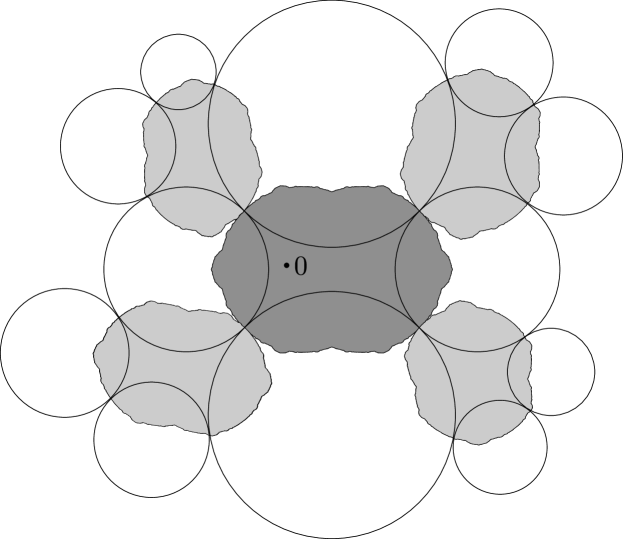
Figure 6.1. A pinched neighborhood of $0$

Local quasiconformal homeomorphism

Let $\mathcal{P}^{\prime}$ be another circle packing with nerve $\mathcal{G}_{i}$. By Proposition 5.10, there exists a quasiconformal map $f_{n}:\widehat{\mathbb{C}}\longrightarrow\widehat{\mathbb{C}}$ with

$$f_{n}(\Lambda(\mathcal{P})\cap\overline{\Omega^{n}})=\Lambda(\mathcal{P}^{\prime})\cap\overline{(\Omega^{\prime})^{n}}$$

so that $\frac{1}{2}\log K(f_{n})=O(\delta^{n})$. Since $D^{n}$ is a finite union of adjacent faces of $\mathcal{G}^{n}_{i}$, the argument applies to $\Delta^{n}$ and we have

Lemma 6.4.

Let $\mathcal{P},\mathcal{P}^{\prime}$ be two circle packings with nerve $\mathcal{G}_{i}$. There exists a quasiconformal map $f_{n}:\widehat{\mathbb{C}}\longrightarrow\widehat{\mathbb{C}}$ with

$$f_{n}(\Lambda(\mathcal{P})\cap\overline{\Delta^{n}})=\Lambda(\mathcal{P}^{\prime})\cap\overline{(\Delta^{\prime})^{n}}$$

so that $\frac{1}{2}\log K(f_{n})=O(\delta^{n})$.

We remark that by definition, these quasiconformal homeomorphism respects the marking, i.e., $f_{n}$ sends a circle $C_{v}$ of $\mathcal{P}$ to the corresponding circle $C^{\prime}_{v}$ of $\mathcal{P}^{\prime}$. Thus, we have the following lemma.

Lemma 6.5.

Suppose that $z\in\Lambda(\mathcal{P})\cap\overline{\Delta^{n}}$. Then $f_{n}(z)=\Psi(z)$.

Möbius approximation

Note that we have $f_{n}(0)=0$. Let $q_{n}=f_{n}^{-1}(1)$ and $p_{n}=f_{n}^{-1}(\infty)$. We define an approximating Möbius map $M_{n}\in\operatorname{PSL}_{2}(\mathbb{C})$ so that

$$M_{n}(0)=0,M_{n}(q_{n})=f_{n}(q_{n})=1,\text{ and }M_{n}(p_{n})=f_{n}(p_{n})=\infty.$$

Denote $a_{n}=M_{n}^{\prime}(0)$, and $X:=\widetilde{\mathbb{C}}-\{0,1,\infty\}$. Let $\epsilon$ be the constant in Lemma 6.3. We assume that $\epsilon\leq\delta$.

Lemma 6.6.

We have $p_{n}^{-1},q_{n}^{-1},a_{n},a_{n}^{-1}=O(\epsilon^{-n})$. Thus, for all $|z|<\epsilon^{3n}$,

$$M_{n}(z)=a_{n}z+O(\epsilon^{2n}|a_{n}z|)=a_{n}z+O(\epsilon^{n}|z|).$$

Proof.

Let $n\geq m$, and consider the map $f_{n}^{-1}\circ f_{m}$. By Lemma 6.3, we can choose points $\alpha_{n},\beta_{n}\in\Lambda(\mathcal{P})\cap\overline{\Delta^{n}}$ with $|\alpha_{n}|=\frac{\epsilon^{n}}{2}$ and $|\beta_{n}|=\epsilon^{n}$. By Lemma 6.5, we have that $f_{n}^{-1}\circ f_{m}$ fixes $0,\alpha_{n},\beta_{n}$. Consider the cross-ratio map $R(z)=(\alpha_{n},\beta_{n};0,z)=\frac{\alpha_{n}}{\beta_{n}}\cdot\frac{z-\beta_{n}}{z-\alpha_{n}}$. By applying Lemma 5.5 to $R\circ f_{n}^{-1}\circ f_{m}$ and $R$, we get

$$d_{X}(\frac{\alpha_{n}}{\beta_{n}}\cdot\frac{p_{m}-\beta_{n}}{p_{m}-\alpha_{n}},\frac{\alpha_{n}}{\beta_{n}}\cdot\frac{p_{n}-\beta_{n}}{p_{n}-\alpha_{n}})=d_{X}(R(p_{m}),R\circ f_{n}^{-1}\circ f_{m}(p_{m}))=O(\delta^{m}).$$

Note that $\frac{p_{m}-\beta_{n}}{p_{m}-\alpha_{n}}\to 1$ as $n\to\infty$, and $\frac{|\alpha_{n}|}{|\beta_{n}|}=\frac{1}{2}$. By fixing $m$ large enough, we can conclude that $\frac{\alpha_{n}}{\beta_{n}}\cdot\frac{p_{n}-\beta_{n}}{p_{n}-\alpha_{n}}$ is close to $\frac{\alpha_{n}}{\beta_{n}}$ for all large $n$. Thus, $\frac{p_{n}-\beta_{n}}{p_{n}-\alpha_{n}}$ is close to $1$ for all sufficiently large $n$. Therefore, $|p_{n}|\geq\epsilon^{n}$ for all sufficiently large $n$. Similarly, we have $|q_{n}|\geq\epsilon^{n}$ for all sufficiently large $n$.

A simple computation shows that $a_{n}=\frac{1}{q_{n}}-\frac{1}{p_{n}}$. Thus, $a_{n}=O(\epsilon^{-n})$. Note that the map $f_{n}^{-1}\circ f_{m}$ sends $0,q_{m},\alpha_{n},p_{m}$ to $0,q_{n},\alpha_{n},p_{n}$. Thus,

$$d_{X}((0,q_{m};\alpha_{n},p_{m}),(0,q_{n};\alpha_{n},p_{n}))=d_{X}(\frac{-\alpha_{n}}{q_{m}-\alpha_{n}}\cdot\frac{p_{m}-q_{m}}{p_{m}},\frac{-\alpha_{n}}{q_{n}-\alpha_{n}}\cdot\frac{p_{n}-q_{n}}{p_{n}})=O(\delta^{m}).$$

We claim that $\frac{|p_{n}-q_{n}|}{|p_{n}q_{n}|}\geq A\epsilon^{n}$ for some $A>0$ and all large $n$. Otherwise, after passing to a subsequence, we have $|\frac{-\alpha_{n}}{q_{m}-\alpha_{n}}\cdot\frac{p_{m}-q_{m}}{p_{m}}|$ behaves like $\epsilon^{n}$, and $|\frac{-\alpha_{n}}{q_{n}-\alpha_{n}}\cdot\frac{p_{n}-q_{n}}{p_{n}}|=O(\epsilon^{2n})$. Since the hyperbolic metric on $X$ near $0$ is bounded below by $\frac{|dx|}{|x||\log|Bx||}$ for some $B>0$ (see e.g. [Hem79, Lemma 2.5]), we have $d_{X}(\epsilon^{n},\epsilon^{2n})$ is bounded below by a constant. This is a contradiction. Thus, we have $a_{n}^{-1}=\frac{p_{n}q_{n}}{p_{n}-q_{n}}=O(\epsilon^{-n})$.

Note $M_{n}(z)=\frac{a_{n}z}{1-\frac{z}{p_{n}}}$. Thus, if $|z|<\epsilon^{3n}$, we have

$$|M_{n}(z)-a_{n}z|=\frac{|\frac{a_{n}z^{2}}{p_{n}}|}{|1-\frac{z}{p_{n}}|}=|a_{n}z|\frac{|\frac{z}{p_{n}}|}{|1-\frac{z}{p_{n}}|}=O(\epsilon^{2n}\cdot|a_{n}z|).$$

Since $|a_{n}|=O(\epsilon^{-n})$, $\epsilon^{2n}|a_{n}z|=O(\epsilon^{n}|z|)$ and the lemma follows. ∎

Lemma 6.7.

For all $\epsilon^{3n+3}\leq|z|\leq\epsilon^{3n}$, we have

$$f_{n}(z)=M_{n}(z)+O(\delta^{n/2}|z|)=a_{n}z+O(\delta^{n/2}|z|).$$

Proof.

We first claim that $a_{n}=O(1)$.

Proof of the claim.

Let $z_{n}\in\Lambda(\mathcal{P})$ with $|z_{n}|=\epsilon^{3n}$. Then by Lemma 6.5, $f_{n-1}(z_{n})=f_{n}(z_{n})$. By Lemma 6.6, $M_{n}(z_{n})=a_{n}z_{n}+O(\epsilon^{2n}|a_{n}z_{n}|)$, so

$$d_{X}(M_{n}(z_{n}),a_{n}z_{n})=O(\epsilon^{2n})=O(\delta^{n}).$$

Similarly, we have that $d_{X}(M_{n-1}(z_{n}),a_{n-1}z_{n})=O(\delta^{n})$. By Lemma 5.5, $d_{X}(f_{n}(z_{n}),M_{n}(z_{n}))=O(\delta^{n})$. Similarly, we have $d_{X}(f_{n-1}(z_{n}),M_{n-1}(z_{n}))=O(\delta^{n})$. Hence, we have

$$d_{X}(a_{n}z_{n},a_{n-1}z_{n})=O(\delta^{n}).$$

Note that near $0$, the hyperbolic metric on $X$ is bounded below by $\frac{|dx|}{|x||\log|Ax||}$ for some $A>0$. By Lemma 6.6, $|\log|a_{n}z_{n}||=O(n)$ and $|\log|a_{n-1}z_{n}||=O(n)$, so the hyperbolic metric between the interval bounded by $|a_{n}z_{n}|$ and $|a_{n-1}z_{n}|$ is bounded below by $\frac{|dx|}{Bn|x|}$ for some $B>0$. Thus

$$O(\delta^{n})=d_{X}(a_{n}z_{n},a_{n-1}z_{n})\geq d_{X}(|a_{n}z_{n}|,|a_{n-1}z_{n}|)\geq\frac{|\log\frac{|a_{n}|}{|a_{n-1}|}|}{Bn}.$$

Hence, $|\log\frac{|a_{n}|}{|a_{n-1}|}|=O(n\delta^{n})=O(\delta^{n/2})$. Therefore, $a_{n}=O(1)$. ∎

By Lemma 6.6, $|M_{n}(z)|\sim|a_{n}z|$, so $|\log|M_{n}(z)||=O(n)$ for all $\epsilon^{3n+3}\leq|z|\leq\epsilon^{3n}$. Thus the hyperbolic metric on the interval between $|M_{n}(z)|/2$ and $2|M_{n}(z)|$ is bounded below by $\frac{|dx|}{Bn|x|}$ for some $B>0$.

Let $\gamma(t),t\in I$ be the hyperbolic geodesic connecting $M_{n}(z)$ and $f_{n}(z)$. We claim that $1/2\leq|\gamma(t)|/|M_{n}(z)|\leq 2$ for all large $n$ and $t\in I$. Without loss of generality, suppose for contradiction that $|\gamma(t)|\geq 2|M_{n}(z)|$. Then

$$d_{X}(\gamma(t),M_{n}(z))\geq d_{X}(|\gamma(t)|,|M_{n}(z)|)\geq d_{X}(2|M_{n}(z)|,|M_{n}(z)|)\geq\frac{\log 2}{Bn}.$$

Thus, $\log 2=O(n\delta^{n})$ which is a contradiction.

Let $|\gamma|$ denote the Euclidean length of $\gamma$. Then $|\gamma|\geq|f_{n}(z)-M_{n}(z)|$. Let $\rho_{X}(x)|dx|$ be the hyperbolic metric on $X$. Note that $\rho_{X}(x)|dx|\geq\frac{|dx|}{2Bn|M_{n}(z)|}$ for all $x\in\gamma$. Therefore, we have

$$d_{X}(f_{n}(z),M_{n}(z))=\int_{\gamma}\rho_{X}(x)|dx|\geq|\gamma|\cdot\frac{1}{2Bn|M_{n}(z)|}\geq\frac{|f_{n}(z)-M_{n}(z)|}{2Bn|M_{n}(z)|}.$$

By Lemma 5.5, $d_{X}(f_{n}(z),M_{n}(z))=O(\delta^{n})$. Thus,

$$|f_{n}(z)-M_{n}(z)|=O(n\delta^{n}|M_{n}(z)|)=O(\delta^{n/2}|z|),$$

where the last equality holds as $a_{n}=O(1)$. By Lemma 6.6, $M_{n}(z)=a_{n}z+O(\epsilon^{n}|z|)$. Since $\epsilon\leq\delta$, we have $f_{n}(z)=a_{n}z+O(\delta^{n/2}|z|)$. ∎

Lemma 6.8.

The derivative $a_{n}=M_{n}^{\prime}(0)$ satisfies $|a_{n}-a_{n-1}|=O(\delta^{n/2})$. In particular, the limit $a=\lim_{n}a_{n}$ exists and $|a-a_{n}|=O(\delta^{n/2})$.

Proof.

Choose a sequence $z_{n}\in\Lambda(\mathcal{P})$ so that $|z_{n}|=\epsilon^{3n}$. By Lemma 6.3, we have $z_{n}\in\overline{\Delta^{n}}$. Therefore, by Lemma 6.5, $\Psi(z_{n})=f_{n}(z_{n})=f_{n-1}(z_{n})$. Hence, by Lemma 6.7,

$$0=\frac{f_{n}(z_{n})-f_{n-1}(z_{n})}{z_{n}}=(a_{n}-a_{n-1})+O(\delta^{n/2}).$$

Therefore, $|a_{n}-a_{n-1}|=O(\delta^{n/2})$. ∎

Proof of asymptotic conformality

We are ready to prove the regularity of local symmetries.

Proof of Theorem 6.1.

Let $z\in\Lambda(\mathcal{P})$ with $\epsilon^{3n+3}\leq|z|\leq\epsilon^{3n}$. By Lemma 6.3, $x\in\overline{\Delta^{3n}}\subseteq\overline{\Delta^{n}}$.

Let $\alpha=\frac{\log\delta}{6\log\epsilon}>0$. Then $\delta^{n/2}=\epsilon^{3n\alpha}=O(|z|^{\alpha})$. By Lemma 6.5, $\Psi(z)=f_{n}(z)$. By Lemma 6.6, Lemma 6.7 and Lemma 6.8, we have

$$\Psi(z)=f_{n}(z) =M_{n}(z)+O(\delta^{n/2}|z|)$$

$$=a_{n}z+O(\delta^{n/2}|z|)$$

$$=az+O(\delta^{n/2}|z|)$$

$$=az+O(|z|^{1+\alpha}).$$

This holds for any $n$, we conclude that $\Psi|_{\Lambda(\mathcal{P})}$ is $C^{1+\alpha}$-conformal at $0$. ∎

6.2. Combinatorially deep points

Let $\mathcal{P}$ be a circle packing with nerve $\mathcal{G}_{i}$. Let $x\in\Lambda(\mathcal{P})\cap\overline{\Pi(\mathcal{P})}$, and let $F^{n}$ be a nested sequence of faces associated to $x$. We say $x$ is a combinatorially deep point if for each $n$, $F^{n+1}\cap\partial F^{n}$ is either empty or a single vertex. We remark that for combinatorially deep points, the corresponding nested sequence is unique. For combinatorially deep points, we can improve the result of asymptotic conformality.

Theorem 6.9.

Let $\mathcal{P}$ and $\mathcal{P}^{\prime}$ be two circle packings with nerve $\mathcal{G}_{i}$, and $\Psi$ be a Teichmüller mapping between them. Then $\Psi$ is $C^{1+\alpha}$-conformal at all combinatorially deep points.

Remark 6.10.

We remark that the assertion of Theorem 6.9 is much stronger than the restriction $\Psi_{\Lambda(\mathcal{P})\cap\overline{\Pi(\mathcal{P})}}$ is $C^{1+\alpha}$-conformal. It asserts that for a combinatorially deep point $x$,

$$\Psi(x+t)=\Psi(x)+\Psi^{\prime}(x)t+O(|t|^{1+\alpha})$$

for all small $t$, while Theorem 6.1 only asserts that for small $t$ with $x+t\in\Lambda(\mathcal{P})\cap\overline{\Pi(\mathcal{P})}$.

In order to control the behavior of points outside the limit set, it is crucial that $\Psi$ is a Teichmüller mapping.

Nested annuli with bounded modulus

Let $\mathcal{P}$ be a circle packing with nerve $\mathcal{G}_{i}$. Let $x$ be a combinatorially deep point, with nested sequence of faces $F^{n}$. In contrast to the pinched neighborhoods that we construct for general points, we can construct a nested neighborhoods of $x$ that are simply connected with good geometric control.

Let $\Omega^{n}=\Omega_{F^{n}}$ be the component of domain of discontinuity associated to $F^{n}$. Since $F^{n}$ and $F^{n+1}$ does not share a common edge, it is easy to see that $\Omega^{n+1}$ is compactly contained in $\Omega^{n}$. Let $A^{n}:=\Omega^{n}-\overline{\Omega^{n+1}}$ be the corresponding annulus. By the Bounded Image Theorem (Theorem 3.3), we have

Lemma 6.11.

The domain $\Omega^{n}$ is a uniform quasi-disk and the annulus $A^{n}$ has uniformly bounded modulus. More precisely, there exists a constant $K,M>1$ so that for each $n\geq 1$,

• $\Omega^{n}$ is a $K$-quasi disk, and

• $\operatorname{Mod}(A_{n})\in[1/M,M]$.

In particular, by compactness, there exists a constant $\epsilon>0$ so that

$$B(0,\epsilon^{n})\subseteq\overline{\Omega^{n}}.$$

Proof of asymptotic conformality at combinatorially deep points

Proof of Theorem 6.9.

Similar as before, by Proposition 5.10, there exists a quasiconformal map $f_{n}:\widehat{\mathbb{C}}\longrightarrow\widehat{\mathbb{C}}$ with

$$f_{n}(\Lambda(\mathcal{P})\cap\overline{\Omega^{n}})=\Lambda(\mathcal{P}^{\prime})\cap\overline{\Omega^{n}}$$

so that $\frac{1}{2}\log K(f_{n})=O(\delta^{n})$. Since $\Psi$ is a Teichmüller mapping, we may choose $f_{n}$ so that

$$\Psi|_{\Omega^{n}}=f_{n}|_{\Omega^{n}}.$$

By replacing the pinched neighborhoods $\Delta^{n}$ and Lemma 6.3 in the proof of Theorem 6.1 by $\Omega^{n}$ and Lemma 6.11, the same arguement proves that $\Psi$ is $C^{1+\alpha}$ at all deep points. ∎

6.3. Renormalization periodic points

In this section, we will study renormalization periodic points. Without loss of generality, let us assume the period is $1$.

First, let $(\mathcal{P}_{0},x_{0})$ be a renormalization fixed point. Let $F^{n}$ be a corresponding nested sequence of faces. We remark that the corresponding nested sequence of faces $F^{n}$ is unique (see Remark 6.14 below). To describe the combinatorics, we give the following definition.

Definition 6.12.

A nested sequence of faces $(F^{n})$ is called a subdivision fixed point if

1. each $F^{n}$ is identified with $F^{0}$, by a cellular homeomorphism

   $$\psi_{n}:F^{0}\longrightarrow F^{n};$$

2. $\psi_{n}\circ\psi_{1}=\psi_{n+1}$ for all $n$.

Proposition 6.13.

Renormalization fixed points are in one to one correspondence with subdivision fixed points.

Proof.

Suppose $(\mathcal{P}_{0},x_{0})$ is a renormalization fixed point. Let $(F^{n})$ be a corresponding nested sequence of faces. Then it is clear that $(F^{n})$ is a subdivision fixed point.

Conversely, let $(F^{n})$ be a subdivision fixed point. By Proposition 5.10, we can find the unique renormalization fixed point by iterating the renormalization operator $\mathfrak{R}$ given by the combinatorial data $(F^{n})$. ∎

Remark 6.14.

Let $(F^{n})$ be a subdivision fixed point. If $F^{1}$ does not share an edge with $F^{0}$. Then $(F^{n})$ gives a combinatorially deep point, and $x_{0}$ is not the tangent point of two circles of $\mathcal{P}_{0}$. If $F^{1}$ shares an edge with $F^{0}$. Then $x_{0}$ is the tangent point of two circles of $\mathcal{P}_{0}$ and is on the boundary $\partial\Pi(\mathcal{P}_{0})$. Thus, in either case, the preimage $\pi^{-1}((\mathcal{P}_{0},x_{0}))\subseteq\widetilde{\Sigma}^{\infty}$ is a singleton.

In the following, we give a more descriptive construction of the renormalization fixed point.

Enlargement of $\mathcal{R}$

Let $(F^{n})$ be a subdivision fixed point. We may assume that $F^{0}=P_{i}$. To construct the renormalization fixed point, we will first construct a new finite subdivision rule $\mathcal{R}^{\prime}$ which enlarges $\mathcal{R}$. This new $\mathcal{R}^{\prime}$ is constructed by adding a new polygon that is inverted copy of $F^{1}$.

More precisely, we define $Q:=\overline{\widehat{\mathbb{C}}-F^{1}}$, and $Q^{\prime}:=\overline{\widehat{\mathbb{C}}-P_{i}}$. Let us denote the subdivision $\mathcal{R}(P_{i})$ as

$$P_{i}=F^{1}\cup\bigcup_{j}P_{i,j}.$$

Then $\bigcup_{j}P_{i,j}\cup Q^{\prime}$ gives a subdivision of $Q$. Since $F^{0}=P_{i}$ and $F^{1}$ are identified by $\psi_{1}$, it induces an identification between $Q$ and $Q^{\prime}$. We remark that this also induces a natural orientation reversing identification of $\partial P_{i}$ with $\partial Q$.

We extend $\mathcal{R}$ to $\mathcal{R}^{\prime}$ so that it consists of $\{P_{1},...,P_{k},Q\}$, where the subdivision $\mathcal{R}^{\prime}(P_{i})=\mathcal{R}(P_{i})$ and $\mathcal{R}^{\prime}(Q)$ as constructed as above. It is easy to see that we can identify each face of the subdivision with a polygon in the list $\{P_{1},...,P_{k},Q\}$, and thus $\mathcal{R}^{\prime}$ is a finite subdivision rule. Since $\mathcal{R}$ is simple, irreducible and acylindrical, it is easy to see that so is $\mathcal{R}^{\prime}$.

$\mathcal{R}^{\prime}$-complex and renormalization fixed point

Let $X$ be the $\mathcal{R}^{\prime}$-complex by gluing $P_{i}$ with $Q$ using the natural orientation reversing identification between $\partial P_{i}$ and $\partial Q$. Then $X$ is homeomorphic to a $2$-sphere.

Let $\mathcal{G}^{n}$ be the 1-skeleton of $\mathcal{R}^{n}(X)$ and $\mathcal{G}=\bigcup_{n}\mathcal{G}^{n}$. Then it is easy to verify that $\mathcal{G}$ is a simple graph. By Theorem E, there exists a unique circle packing $\mathcal{P}$ with nerve $\mathcal{G}$.

Let $\mathcal{G}_{F^{n}}=\mathcal{G}\cap F^{n}$, where $F^{n}$ is naturally identified as a subset of $P_{i}$. By construction, it is easy to see that there exists a homeomorphism $\tilde{\phi}$ of $\mathcal{G}$ extending the local homeomorphism $\mathcal{G}_{F^{1}}\longrightarrow\mathcal{G}_{F^{0}}$. Thus, by Theorem E, there exists a Möbius map $\phi$ that fixes $\mathcal{P}$.

Let $\mathcal{P}_{0}$ be the sub-circle packing of $\mathcal{P}$ associated to $\mathcal{G}_{F^{0}}$, and $x_{0}$ is the repelling fixed point of $\phi$. Then it is easy to see that $(\mathcal{P}_{0},x_{0})$ is the corresponding renormalization fixed point.

6.4. Proof of Theorem D

We are now ready to assemble the proof of the universality and regularity theorem.

Proof of Theorem D.

The statement (1) follows from Theorem 6.1, and the statement (2) follows from the above discussion.

By Remark 6.14, $x_{0}$ is either a combinatorially deep point, or a cusp point on the boundary $\partial\Pi(\mathcal{P}_{0})$. In the first case, we have that the scaling factor $|\mu|>1$ by Lemma 6.11. In the second case, the Möbius map $\phi$ preserves the two circles in $\mathcal{P}_{0}$ that passes through $x_{0}$. Thus $\phi$ is a parabolic map with a fixed point at $x_{0}$. This proves (3).

The last statement follows from the fact that the map $\Psi|_{\Lambda(\mathcal{P}_{0})\cap\overline{\Pi(\mathcal{P}_{0})}}$ is $C^{1+\alpha}$-conformal. ∎

7. Generalizations of subdivision rules

In this section, we will explain how our methods can be generalized for graphs with other types of subdivision rules.

7.1. Interpolations of finite subdivision rules

In this section, we generalize the finite subdivision rules. This generalization allows us to study subdivisions that are not periodic, and can be regarded as the interpolation of multiple finite subdivision rules.

Definition 7.1.

An interpolation of finite subdivision rules $\mathcal{R}$ consists of

1. a finite collection of polygons $\{P_{i}:i=1,...,k\}$;

2. a subdivision $\mathcal{R}(P_{i})$ that decomposes each polygon $P_{i}$ into $m_{i}\geq 2$ closed 2-cells

   $$P_{i}=\bigcup_{j=1}^{m_{i}}P_{i,j}$$

   so that each edge of $\partial P_{i}$ contains no vertices of $\mathcal{R}(P_{i})$ in its interior;

3. a finite collection of cellular maps $\psi_{i,j,l},l=1,...,k_{i,j}$ for $P_{i,j}$ so that

   $$\psi_{i,j,l}:P_{\sigma(i,j,l)}\longrightarrow P_{i,j}$$

   are homeomorphisms between the open 2-cells.

Remark 7.2.

We remark that the difference between an interpolation of finite subdivision rules and a finite subdivision rule is in the condition $(3)$. For a finite subdivision rule, there is a unique identification between a face of the subdivision with a polygon in the original list, while an interpolation of finite subdivision rules allows multiple different ways of identifications.

Let $\mathcal{R}$ be an interpolation of finite subdivision rules. Let $\mathcal{R}(P_{i})$ be the subdivision of $P_{i}$ and $\mathcal{G}^{1}_{i}$ be the corresponding 1-skeleton.

Definition 7.3.

Let $\mathcal{R}$ be an interpolation of finite subdivision rules. We say it is

• simple if for each $i$, $\mathcal{G}^{1}_{i}$ is simple;

• irreducible if for each $i$, $\partial P_{i}$ is an induced subgraph of $\mathcal{G}^{1}_{i}$;

• acylindrical if for each $i$, each face of $\mathcal{R}(P_{i})$ is a Jordan domain, and the face $P_{i}$ is acylindrical in $\mathcal{G}^{1}_{i}$.

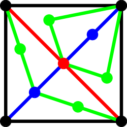
Figure 7.1. The first few levels of an interpolation of the two finite subdivision rules shown in Figure 1.1. Note that this example is not acylindrical.

Let $P\in\{P_{1},...,P_{k}\}$ be a polygon. To iterate $\mathcal{R}$ on $P$, we need to make a choice of the identification of the face of $\mathcal{R}(P)$ with a polygon in $\{P_{i}:i=1,...,k\}$. Suppose that such a choice is made at every iteration. Abusing the notations, we denote the sequence of subdivisions by $\mathcal{R}^{n}(P)$. Let $\mathcal{G}^{n}$ be the 1-skeleton of $\mathcal{R}^{n}(P)$, and $\mathcal{G}$ be the direct limit of $\mathcal{G}^{n}$. Let $F$ be the external face for $\mathcal{G}$.

We call the infinite graph $\mathcal{G}$ an admissible subdivision graph for $\mathcal{R}$. We remark that there can be uncountably many different admissible subdivision graph for $\mathcal{R}$.

The same proof as Theorem A gives the following.

Theorem 7.4.

Let $\mathcal{R}$ be a simple, irreducible, acylindrical interpolation of finite subdivision rules. Let $\mathcal{G}$ be an admissible subdivision graph for $\mathcal{R}$. Then the moduli space $\mathcal{M}(\mathcal{G})$ is isometrically homeomorphic to $\operatorname{Teich}(\Pi_{F})$. In particular, any two circle packings with nerve $\mathcal{G}$ are quasiconformally homeomorphic.

Given a sequence of nested faces for $\mathcal{G}$, we can define the corresponding iteration of renormalizations $\mathfrak{R}^{n}$. The same proof of Theorem C also gives

Theorem 7.5.

Let $\mathcal{R}$ be an interpolation of finite subdivision rules. There exist a constant $\delta<1$ and $C$ such that the following holds.

Let $\mathcal{G}$ be an admissible subdivision graph for $\mathcal{R}$.

• (Finite approximation) Suppose $\mathcal{P},\mathcal{P}^{\prime}\in\mathcal{M}(\mathcal{G}^{n+k})$ have the same external class. Let $\mathcal{P}^{k},(\mathcal{P}^{\prime})^{k}$ be the sub-circle packing associated to $\mathcal{G}^{k}$. Then

  $$d(\mathcal{P}^{k},(\mathcal{P}^{\prime})^{k})\leq\delta^{n-1}\min\{d(\mathcal{P},\mathcal{P}^{\prime}),C\}=O(\delta^{n}).$$

• (Renormalization) Let $\mathcal{P},\mathcal{P}^{\prime}\in\mathcal{M}(\mathcal{G})$. Then given a sequence of nested faces for $\mathcal{G}$, we have

  $$d(\mathfrak{R}^{n}((\mathcal{P},x)),\mathfrak{R}^{n}((\mathcal{P}^{\prime},x^{\prime})) \leq\delta^{n-1}d(\mathfrak{R}((\mathcal{P},x)),\mathfrak{R}((\mathcal{P}^{\prime},x^{\prime}))$$

  $$\leq\delta^{n-1}\min\{d((\mathcal{P},x),(\mathcal{P}^{\prime},x^{\prime})),C\}$$

  $$=O(\delta^{n}).$$

7.2. $\mathbb{Z}^{2}$-subdivision rules

In this subsection, we discuss what happens if the subdivision rule is not finite. We illustrate the ideas using a special type of subdivision rules, called $\mathbb{Z}^{2}$-subdivision rule. Such subdivision rules arise naturally from rank 2 cusps of a Kleinian groups, and will be applied in §8.

$\mathbb{Z}^{2}$-tilings

A CW-complex $X$ that is homeomorphic to $\mathbb{C}$ is called a $\mathbb{Z}^{2}$-tiling if there exists a properly discontinuous action of $\mathbb{Z}^{2}$. Note that each element of $\mathbb{Z}^{2}$ is a cellular homeomorphism of $X$, thus $X$ necessarily contains infinitely many 2-cells.

Let $P$ be a fundamental domain for this $\mathbb{Z}^{2}$-action, which we assume to be a Jordan domain. Let $Q=\overline{\widehat{\mathbb{C}}-P}$ be the complementary polygon associated to $P$. Then the $\mathbb{Z}^{2}$-tiling generates a subdivision of $Q$. More precisely, we can write

$$Q=\overline{\bigcup_{g\in\mathbb{Z}^{2}-\{id\}}g\cdot P},$$

where $(g\cdot\operatorname{Int}(P))\cap(g^{\prime}\cdot\operatorname{Int}(P))=\emptyset$ if $g\neq g^{\prime}$. We remark that technically, this is a subdivision of the punctured polygon $Q^{*}:=Q-\{\infty\}$. To avoid complicated notations, we will abuse the terminology and simply call it a subdivision of $Q$.

$\mathbb{Z}^{2}$-subdivisions

A $\mathbb{Z}^{2}$-subdivision rule is a generalization of a finite subdivision rule, that allows infinitely many faces in the subdivision.

Definition 7.6.

A $\mathbb{Z}^{2}$-subdivision rule $\mathcal{R}$ consists

1. a finite collection of polygons $\{P_{1},...,P_{k},Q_{1},...,Q_{l}\}$ with $l\leq k$ and $Q_{i}=\overline{\widehat{\mathbb{C}}-P_{i}}$ is the complementary polygon of $P_{i}$;

2. a subdivision $\mathcal{R}(P_{i})$ that decomposes each polygon $P_{i}$ into at least two closed 2-cells

   $$P_{i}=\bigcup_{j=1}^{m_{i}}P_{i,j}\cup\bigcup_{j=1}^{n_{i}}Q_{i,j}$$

   so that each edge of $\partial P_{i}$ contains no vertices of $\mathcal{R}(P_{i})$ in its interior;

3. a collection of cellular maps, denoted by

   $$\psi_{i,j}:P_{\sigma(i,j)}\longrightarrow P_{i,j},\;\;\phi_{i,j}:Q_{\tau(i,j)}\longrightarrow Q_{i,j}$$

   that are homeomorphisms between the open 2-cells;

4. a $\mathbb{Z}^{2}$-tiling $X_{i}$ with fundamental domain $P_{i}$ which induces a subdivision $\mathcal{R}(Q_{i})$ by

   $$Q_{i}=\overline{\bigcup_{g\in\mathbb{Z}^{2}-\{id\}}g\cdot P_{i}},$$

   where each closed 2-cell of $\mathcal{R}(Q_{i})$ is naturally identified with $P_{i}$.

Similar as a finite subdivision rule, we can iterate this procedure. We define $\mathcal{G}^{n}_{i}$ and $\mathcal{H}^{n}_{i}$ as the 1-skeleton of $\mathcal{R}^{n}(P_{i})$ and $\mathcal{R}^{n}(Q_{i})$ respectively. Let $\mathcal{G}_{i}=\bigcup_{n}\mathcal{G}^{n}_{i}$ and $\mathcal{H}_{i}=\bigcup_{n}\mathcal{H}^{n}_{i}$. We say $\mathcal{R}$ is simple if $\mathcal{G}_{i}$ and $\mathcal{H}_{i}$ are simple.

Following the discussion in §4.1, we say $\mathcal{R}$ is acylindrical if

• each face of $\mathcal{G}^{1}_{i}$ is a Jordan domain;

• the subgraph $\mathcal{G}^{0}_{i}$ is acylindrical in $\mathcal{G}^{1}_{i}$.

We remark that by our definition, the above two properties hold automatically for $\mathcal{H}^{1}_{i}$ and $\mathcal{H}^{0}_{i}$.

We can define an $\mathcal{R}$-complex $X$ similar as in the case of finite subdivision rule. If $X$ is homeomorphic to the Riemann sphere $\widehat{\mathbb{C}}$, we say the corresponding graph $\mathcal{G}=\bigcup_{n}\mathcal{G}^{n}$ a spherical subdivision graph with $\mathbb{Z}^{2}$-subdivision rule.

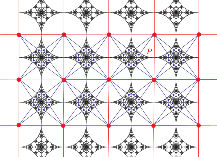
Figure 7.2. An example of a subdivision graph for a $\mathbb{Z}^{2}$-subdivision rule with the associated circle packing, given by a Kleinian group

Existence and rigidity of $\mathbb{Z}^{2}$-subdivision rule

Theorem 7.7.

Let $\mathcal{R}$ be a simple acylindrical $\mathbb{Z}^{2}$-subdivision rule.

• The moduli space $\mathcal{M}(\mathcal{G}_{i})$ is isometrically homeomorphic to $\operatorname{Teich}(\Pi_{F_{i}})$, where $F_{i}$ is the external face of $\mathcal{G}_{i}$.

• Suppose $\mathcal{G}$ is a simple spherical subdivision graph with $\mathbb{Z}^{2}$-subdivision rule $\mathcal{R}$. Then there exists a unique circle packing $\mathcal{P}$ whose nerve is $\mathcal{G}$.

We remark that with some minor adjustments, the proof is almost identical to the case of a finite subdivision rule. We will only sketch the proof and emphasize the one subtle difference here.

Consider the graph $\mathcal{H}^{1}_{i}$. Note that it is simply the 1-skeleton of a $\mathbb{Z}^{2}$-tiling, thus it is easy to construct circle packings with nerve $\mathcal{H}^{1}_{i}$. Each face of $\mathcal{H}^{1}_{i}$ can be identified with $P_{i}$. Hence, for each face $F$, we can construct a map

$$\pi_{F}:\mathcal{M}(\mathcal{H}^{1}_{i})\longrightarrow\operatorname{Teich}(\Pi_{P_{i}}).$$

Similar as in §5.1, we can construct a compact set $K_{i}\subseteq\operatorname{Teich}(\Pi_{P_{i}})$. Consider the set

$$\mathcal{M}_{K_{i}}(\mathcal{H}^{1}_{i})=\{\mathcal{P}\in\mathcal{M}(\mathcal{H}^{1}_{i}):\pi_{F}(\mathcal{P})\in K_{i}\text{ for all faces }F\}.$$

Let

$$\rho_{Q_{i}}=\pi_{Q_{i}}\circ\tau_{\mathcal{H}^{0}_{i},\mathcal{H}^{1}_{i}}:\mathcal{M}(\mathcal{H}^{1}_{i})\longrightarrow\operatorname{Teich}(\Pi_{Q_{i}})$$

be the composition of a projection map with the skinning map.

Lemma 7.8.

Let $\mathcal{P}_{1},\mathcal{P}_{2}\in\mathcal{M}_{K_{i}}(\mathcal{H}^{1}_{i})$. Then there exists a constant $\delta$ so that

$$d(\rho_{Q_{i}}(\mathcal{P}_{1}),\rho_{Q_{i}}(\mathcal{P}_{2}))\leq\delta\cdot d(\mathcal{P}_{1},\mathcal{P}_{2})=\delta\cdot\sup_{F}d(\pi_{F}(\mathcal{P}_{1})),\pi_{F}(\mathcal{P}_{2})).$$

Proof.

Since $\pi_{F}(\mathcal{P}_{1})$ (and $\pi_{F}(\mathcal{P}_{2})$) is contained in a compact set, $\mathcal{P}_{1}$ and $\mathcal{P}_{2}$ are quasiconformally homeomorphic. It follows from the discussion in [He91, §3] that the limit set of the group generated by reflection along circles in $\mathcal{P}_{1}$ (and $\mathcal{P}_{2}$) has zero measure. Therefore $d(\mathcal{P}_{1},\mathcal{P}_{2})=\sup_{F}d(\pi_{F}(\mathcal{P}_{1})),\pi_{F}(\mathcal{P}_{2}))\leq C_{i}$, where $C_{i}$ is the diameter of $K_{i}$.

Let $F_{ext}$ be the external face of $\mathcal{H}^{1}_{i}$. Then $\mathcal{H}^{1}_{i}=\bigcup_{g\in\mathbb{Z}^{2}}g\cdot\partial F_{ext}$. To get the uniform contraction, we can consider the subgraph

$$\mathcal{H}^{1}_{i}(3)=\bigcup_{g=(a,b),|a|,|b|\leq 1}g\cdot\partial F_{ext}.$$

Let $H$ be the unique face of $\mathcal{H}^{1}_{i}(3)$ that is not a face of $\mathcal{H}^{1}_{i}$.

Since $d(\mathcal{P}_{1},\mathcal{P}_{2})\leq C_{i}$, the diameter of $\rho_{H}(\mathcal{M}_{K_{i}}(\mathcal{H}^{1}_{i}))=\pi_{H}\circ\tau_{\mathcal{H}^{1}_{i}(3),\mathcal{H}^{1}_{i}}(\mathcal{M}_{K_{i}}(\mathcal{H}^{1}_{i}))$ is bounded by $C_{i}$, and hence it is contained in some compact set $K_{H}\subseteq\operatorname{Teich}(\Pi_{H})$. Consider the map $\pi_{Q_{i}}\circ\tau_{\mathcal{H}^{0}_{i},\mathcal{H}^{1}_{i}(3)}:\mathcal{M}(\mathcal{H}^{1}_{i}(3))=\operatorname{Teich}(\Pi_{P_{i}})^{9}\times\operatorname{Teich}(\Pi_{H})\longrightarrow\operatorname{Teich}(\Pi_{P_{i}})$. Thus, there exists $\delta<1$ so that

$$|d(\pi_{Q_{i}}\circ\tau_{\mathcal{H}^{0}_{i},\mathcal{H}^{1}_{i}(3)})|\leq\delta$$

on the compact set $K_{i}^{9}\times K_{H}\subseteq\operatorname{Teich}(\Pi_{P_{i}})^{9}\times\operatorname{Teich}(\Pi_{H})$. The lemma now follows from a similar argument as in Lemma 5.2. ∎

Proof of Theorem 7.7.

The existence part follows by a similar argument as in Theorem 4.1 by taking geometric limit of finite circle packings.

To prove the uniqueness, let $\mathcal{P}_{1},\mathcal{P}_{2}\in\mathcal{M}(\mathcal{G}_{i})$ be two circle packings with the same external class. Let $\mathcal{P}^{n}_{i}$ be the sub-circle packings of $\mathcal{P}_{i}$ associated to $\mathcal{G}^{n}_{i}$. By applying Theorem 3.3 to subdivisions of $P_{i}$, and combining Corollary 5.3 and Lemma 7.8, the same argument as in Theorem 5.6 gives

$$d(\mathcal{P}^{n}_{1},\mathcal{P}^{n}_{2})=O(\delta^{n}).$$

Since this is true for any $n$, we conclude that $\mathcal{P}_{1},\mathcal{P}_{2}$ are conformally homeomorphic.

A similar argument also allows us to prove the case for graph $\mathcal{G}$. ∎

8. Kleinian circle packings

Throughout this section, let $\Gamma$ be a Kleinian group, $\Lambda$ its limit set, and $\Omega$ the domain of discontinuity. We also use $M=\Gamma\backslash\mathbb{H}^{3}$ to denote the corresponding hyperbolic 3-manifold.

The goal of this section is twofold. First, we give a topological description of the hyperbolic 3-manifold $M$ when its limit set comes from a circle packing, and in particular prove the following result.

Theorem 8.1.

Let $\mathcal{P}$ be a Kleinian circle packing with nerve $\mathcal{G}$. Let $\Gamma$ be the associated Kleinian group, and $M=\Gamma\backslash\mathbb{H}^{3}$ the corresponding hyperbolic 3-manifold. Suppose $\Gamma$ is geometrically finite. Then $M$ is acylindrical, and homeomorphic to the interior of a compression body with empty or only toroidal interior boundary components.

As a matter of fact, we prove a more general topological characterization that includes all finitely generated Kleinian groups whose limit set is the limit set of a circle packing. Using this characterization, our second goal is to show the following, using mostly topological arguments.

Theorem 8.2.

Let $\mathcal{P}$ be a Kleinian circle packing. Let $\Gamma$ be the corresponding Kleinian group. Then its nerve $\mathcal{G}$ is a spherical subdivision graph

• for a finite subdivision rule if and only if $\Gamma$ is geometrically finite and contains no rank-2 parabolic subgroup;

• for a $\mathbb{Z}^{2}$-subdivision rule if and only if $\Gamma$ is geometrically finite and contains at least one rank-2 parabolic subgroup.

Combined with Theorem E (without rank-2 cusps) or Theorem 7.7 (with rank-2 cusps), we immediately obtain Theorem G. Note that we need not check acylindricity of the subdivision rule, since a circle packing already exists.

8.1. Geometric finiteness and acylindricity

In this section, we recall some basic facts regarding geometrically finite, acylindrical hyperbolic 3-manifolds.

Recall that a Kleinian group $\Gamma$ (and the corresponding hyperbolic 3-manifold $M$) is called geometrically finite if there exists a finite-sided fundamental polyhedron for the action of $\Gamma$ on $\mathbb{H}^{3}$. Equivalently, the unit neighborhood of the convex core of $M$

$$\operatorname{core}(M):=\Gamma\backslash\operatorname{Cvx\,Hull}(\Lambda)$$

has finite volume.

We have discussed incompressibility and acylindricity in the context of kissing reflection groups, cf. §3. In general, let $(N,P)$ be a pared 3-manifold, where $N$ is a compact oriented 3-manifold with boundary, and $P\subseteq\partial N$ is a submanifold consisting of incompressible tori and annuli. See [Thu86] for a precise definition in arbitrary dimension. Set $\partial_{0}N=N-P$. Then we say $(N,P)$ is acylindrical if each component of $\partial_{0}N$ is incompressible, and every essential cylinder with both ends in $\partial_{0}N$ is boundary parallel.

For a geometrically finite $M$, let $\operatorname{core}_{\epsilon}(M)$ be the convex core of $M$ minus $\epsilon$-thin cuspidal neighborhoods for all cusps. Here $\epsilon$ is always chosen small enough, say smaller than the Margulis constant in dimension 3. Let $P\subseteq\partial\operatorname{core}_{\epsilon}(M)$ be the union of boundaries of all cuspidal neighborhoods, then $(\operatorname{core}_{\epsilon}(M),P)$ is a pared 3-manifold, and we say $M$ (and the corresponding Kleinian group $\Gamma$) is acylindrical if $(\operatorname{core}_{\epsilon}(M),P)$ is. Note that the connected components of $\partial\operatorname{core}_{\epsilon}(M)-P$ are in one-to-one correspondence with the boundary components of the Kleinian manifold $\overline{M}$. In this way, it is easy to reconcile the general definition here with the one given in §3.

One can recognize acylindricity from the limit set in the geometrically finite case, in the spirit of Theorems 3.4 and 3.5. We start with the following lemma:

Lemma 8.3.

Let $\Gamma$ be any nonelementary Kleinian group, and $\Omega_{1}$, $\Omega_{2}$ two connected components of its domain of discontinuity $\Omega$. Let $\Gamma_{i}$ be the stabilizer of $\Omega_{i}$ in $\Gamma$, and assume $X_{i}:=\Gamma_{i}\backslash\Omega_{i}$ is a Riemann surface of finite type. Suppose $\overline{\Omega_{1}}\cap\overline{\Omega_{2}}$ consists of one point $p$. Then

1. $p$ is a parabolic fixed point;

2. Let $\sigma_{i}$ be a curve on $X_{i}$ that is not null-homotopic in $\overline{M}:=\Gamma\backslash\{\mathbb{H}^{3}\cup\Omega\}$. Then $\sigma_{1}$ and $\sigma_{2}$ are not homotopic in $\overline{M}$.

Proof.

By [Mas74, Theorem 3], $p=\overline{\Omega_{1}}\cap\overline{\Omega_{2}}=\Lambda(\Gamma_{1}\cap\Gamma_{2})$, so it must be a parablic fixed point. Moreover, if two curves $\sigma_{1}$ and $\sigma_{2}$ are homotopic, then $\Gamma_{1}\cap\Gamma_{2}$ contains a hyperbolic element, and thus $\overline{\Omega_{1}}\cap\overline{\Omega_{2}}$ contains at least two points. ∎

Proposition 8.4 (Characterization of geom. finite acy. Kleinian groups).

Suppose $\Gamma$ is nonelementary and geometrically finite of infinite volume. Then $\Gamma$ is acylindrical if and only if any connected component of the domain of discontinuity $\Omega$ is a Jordan domain, and the closures of any pair of connected components share at most one point. Moreover, any common point of the closures of two connected components is a parabolic fixed point, and any rank-1 parabolic fixed point arises this way.

Proof.

For the “only if” and the “moreover” part, see [BO22, Lemma 11.2]. For the “if” part, note that each boundary component of $\overline{M}$ is incompressible since each component of $\Omega$ is simply connected. Moreover, $\overline{M}$ is acylindrical, for any essential cylinder gives curves on $\partial_{0}N$ violating Part (2) of the previous lemma. ∎

Recall that the quasiconformal deformation space $\mathcal{QC}(\Gamma)$ can be identified with the Teichmüller space $\mathcal{T}(\partial\overline{M})$ if every boundary component is incompressible. Moreover, when $\Gamma$ is acylindrical, there exists a unique geometrically finite $\Gamma^{\prime}\in\mathcal{QC}(\Gamma)$ so that the convex core of the corresponding 3-manifold has totally geodesic boundary [McM90, Corollary 4.3]. This implies the limit set $\Lambda$ of $\Gamma$ is quasiconformally homeomorphic to the complement of countably many open round disks.

8.2. Compression bodies and gasket limit sets

In this section, we describe what hyperbolic 3-manifolds associated to Kleinian circle packings look like. In fact, we work in a more general setting and consider Kleinian groups with gasket limit sets. Here, a gasket is a closed subset of $\hat{\mathbb{C}}$ so that

1. each complementary component is a Jordan domain;

2. any two complementary components touch at most at 1 point;

3. no three complementary components share a boundary point;

4. the nerve, obtained by assigning a vertex to each complementary component and an edge if two touch, is connected.

Clearly the limit set of a circle packing is a gasket.

For the remainder of this subsection, we assume $\Gamma$ is finitely generated, whose limit set $\Lambda$ is a gasket with nerve $\mathcal{G}$. Let $\operatorname{core}^{\prime}_{\epsilon}(M)$ be the convex core of the corresponding hyperbolic 3-manifold $M$ minus $\epsilon$-thin cuspidal neighborhoods for all cusps of rank $1$. We will show

Proposition 8.5.

The manifold $M$ is homeomorphic to the interior of a compression body $(N,\partial N)$, with exterior boundary $\partial_{e}N$ homeomorphic to $S=\partial\operatorname{core}^{\prime}_{\epsilon}(M)$.

Compression bodies

A compact, orientable, irreducible manifold with boundary $(N,\partial N)$ is called a compression body if it is homeomorphic to the boundary connected sum of a solid 3-ball with a collection of solid tori and a collection of trivial interval bundles over closed surfaces, so that the other summands are attached to the 3-ball along disjoint disks. Either collection may be empty.

For one boundary component $\partial_{e}N$ of $N$, the inclusion induces a surjection on $\pi_{1}$; we refer to this component as the exterior boundary. As a matter of fact, this characterizes compression bodies: $(N,\partial N)$ is a compression body if and only if the inclusion of one component of $\partial N$ induces a surjection on $\pi_{1}$ (see e.g. [BJM13, Lem. 4.1]). All other boundary components of $N$ are incompressible; we refer to them as interior boundary components.

More generally, a punctured compression body also allows in the definition above gluing trivial interval bundles over punctured surfaces. In this case, the exterior boundary is a punctured surface, so are some of the interior boundary components. It is easy to see that the characterization mentioned above still applies in this general situation. From now on for simplicity, when we use “compression body”, the punctured case is also included.

A result of Otal, called “disk-busting” [Ota88, Rem. 1.5], gives a criterion for $(N,P)$ to be a pared acylindrical manifold, where $P$ is the union of all toroidal boundary components and a collection of simple curves on $\partial_{e}N$.

Gasket limit sets

We are now ready to prove Proposition 8.5. We start with the following lemma.

Lemma 8.6.

The boundary $S:=\partial\operatorname{core}^{\prime}_{\epsilon}(M)$ is connected, and the map $\pi_{1}(S)\to\pi_{1}(M)$ induced by inclusion is a surjection.

Proof.

Note that $X:=\Gamma\backslash\Omega$ is a union of finite area hyperbolic surfaces by the Ahlfors finiteness theorem. Components of $X$ are in one-to-one correspondence with components of $\partial\operatorname{core}(M)$. Moreover, $\partial\operatorname{core}(M)\cap\partial\operatorname{core}_{\epsilon}^{\prime}(M)$ consists of $\epsilon$-thick parts of components of $\partial\operatorname{core}(M)$, and $\partial\operatorname{core}_{\epsilon}^{\prime}(M)-\partial\operatorname{core}(M)$ consists of boundaries of cuspidal neighborhoods.

Each component $\widetilde{S^{\prime}}$ of $\partial\operatorname{Cvx\,Hull}(\Omega)$ faces a component $\Omega^{\prime}$ of $\Omega$, and covers a component $S^{\prime}$ of $\partial\operatorname{core}(M)$. The $\epsilon$-part of $S^{\prime}$ is covered by $\widetilde{S^{\prime}}$ minus disjoint horoballs based at all the parabolic fixed points on $\partial\Omega^{\prime}$. Note that by Lemma 8.3, these in particular include all common boundary points between $\Omega^{\prime}$ and another component of $\Omega$. In fact by Proposition 8.4, in the geometrically finite case, parabolic fixed points on $\partial\Omega^{\prime}$ are precisely common boundary points, but in general the former also include singly cusped parabolic points.

Furthermore, lifts of each component of $\partial\operatorname{core}_{\epsilon}^{\prime}(M)-\partial\operatorname{core}(M)$ are either flat strips bounded by two horocycles based at a parabolic fixed point at infinity (when the parabolic fixed point is a common boundary point), or half planes bounded by a single horocycle (when the parabolic fixed point is singly cusped).

Thus the preimage of $S$ under the projection $\pi:\mathbb{H}^{3}\to M$ can be described as follows. Take $\partial\operatorname{Cvx\,Hull}(\Omega)$, minus a horoball based at each parabolic fixed point, and then add back the flat strips or half planes on those horoballs contained in $\operatorname{Cvx\,Hull}(\Omega)$. Note that for any pair of components $\Omega^{\prime},\Omega^{\prime\prime}$ of $\Omega$ sharing a common boundary point, the corresponding components $\widetilde{S^{\prime}},\widetilde{S^{\prime\prime}}$ of $\partial\operatorname{Cvx\,Hull}(\Omega)$ are connected by a strip. As the nerve $\mathcal{G}$ is connected, this implies that $\pi^{-1}(S)$ is connected, and hence $S$ is connected as well.

Finally note that $\Gamma$ acts on $\pi^{-1}(S)$ freely and properly discontinuously. Hence $\Gamma\cong\pi_{1}(M)$ is a quotient of $\pi_{1}(S)$, as desired. ∎

Proof of Proposition 8.5.

By the tameness theorem of Agol [Ago04] and Calegari-Gabai [CG06], $M$ is homeomorphic to the interior of a compact 3-manifold with boundary $N$. If there are any singly cusped parabolic points, we modify $N$ by deleting an annular neighborhood on $\partial N$ of the corresponding simple curve representing the parabolic element.

By the previous lemma, one boundary component of $N$ induces a surjection on $\pi_{1}$, so $N$ must be a compression body, as desired. ∎

Moreover, we note that any non-toroidal interior boundary component of $N$ must correspond to a geometrically infinite end of $M$, for otherwise the limit set is not a gasket. Also, as singly cusped parabolic points only exist when $M$ is geometrically infinite, $N$ is compact (i.e. not punctured) when $M$ is geometrically finite. Thus we have the following corollary:

Corollary 8.7.

The 3-manifold $M$ is geometrically finite if and only if the interior boundary of $N$ is empty or consists entirely of tori. Moreover, in this case

• the compression body $N$ is compact;

• the 3-manifold $M$ is acylindrical; and hence

• the limit set $\Lambda$ is quasiconformally homeomorphic to the limit set of a Kleinian circle packing.

Proof.

The fact that $M$ is acylindrical follows from Proposition 8.4, and the last statement then follows from [McM90, Cor. 4.3]. ∎

So as soon as we have a geometrically finite gasket limit set, we can quasiconformally deform it to obtain a circle packing. In practice, it is much easier to construct geometrically finite Kleinian circle packings directly, e.g. the Apollonian gasket, and many examples studied in [LLM22].

Topology from the nerve.

We want to extract more topological information about the 3-manifold from the nerve. For example, is it possible to see whether the interior boundary of the compression body $N$ is empty from $\mathcal{G}$? Since the topology of $(N,\partial N)$ determines many geometric properties of $M$ (e.g. geometric finiteness by Corollary 8.7), this is the same as asking if these geometric properties can be read from $\mathcal{G}$.

By the discussion above, four distinct cases arise:

1. The interior boundary of $N$ is empty, i.e. $N$ is a handlebody;

2. The interior boundary of $N$ consists only of tori;

3. $N$ is homeomorphic to $\partial_{e}N\times[0,1]$;

4. The interior boundary of $N$ has at least one non-toroidal component, and $N$ is not homeomorphic to $\partial_{e}N\times[0,1]$.

The first two cases are closely related to subdivisions, and will be treated in the next subsection. We can distinguish the third case easily from the graph $\mathcal{G}$:

Proposition 8.8.

The compression body $N$ is homeomorphic to $\partial_{e}N\times[0,1]$ if and only if $\mathcal{G}$ is a tree. In this case, $M$ has a geometrically finite end and an geometrically infinite end.

Proof.

Note that in the proof of Lemma 8.6, $\pi^{-1}(S)$ is simply connected if and only if $\mathcal{G}$ is a tree, and thus $\Gamma\cong\pi_{1}(S)$ if and only if $\mathcal{G}$ is a tree.

Moreover, $\Gamma\backslash\Omega$ corresponds to a geometrically finite end of $M$. The other end must be geometrically infinite, for otherwise some component of $\Omega$ meets others in infinitely many points. ∎

It is easy to see that for the last case, we can find a collection of compressing disks to cut off non-toroidal interior boundary components. The structure of the nerve graph is thus a hybrid of the geometrically finite case and the tree case. We will remark on this case in greater detail later.

We remark that we can construct examples of Kleinian circle packings whose nerve is a tree. Indeed, Let $S$ be a surface of genus $g\geq 2$, and $\mu$ a maximal collection of disjoint simple closed curve on $S$ (in particular $S-\mu$ is a collection of pairs of pants), and $\lambda$ a minimal lamination so that $S-\lambda$ consists of ideal polygons. By [NS12, Theorem 1.3], there exists a Kleinian surface group with ending lamination $\lambda$, and parabolic locus $\mu$. The convex core boundary consists of three-punctured spheres, so must be totally geodesic. Therefore each domain of discontinuity is a round disk. As mentioned in the introduction, varying $\lambda$ while fixing $\mu$ gives conformally different packings with the same nerve, so no rigidity can be obtained in general for this case.

An entirely analogous construction also provides many examples for the last case, again applying [NS12, Theorem 1.3].

8.3. Kleinian subdivision rules

In this subsection, we associate a finite or $\mathbb{Z}^{2}$-subdivision rule $\mathcal{R}$ to the nerve $\mathcal{G}$ of the gasket limit set of a geometrically finite Kleinian group $\Gamma$.

The proof comes in two steps: we first reduce the question to a topological problem, and then show that this topological problem can always be solved in our setting. Note that by Corollary 8.7, we may assume the gasket comes from a circle packing $\mathcal{P}$, but this extra assumption is non-essential.

By Proposition 8.5, the hyperbolic 3-manifold $M=\Gamma\backslash\mathbb{H}^{3}$ is homeomorphic to the interior of a compact compression body $N$ whose interior boundary is either empty or consists of tori. Moreover, a collection of disjoint simple closed curves $\{\gamma_{i}\}$ on $\partial_{e}N$ gives the parabolic locus $P=\sqcup P_{i}$, where each $P_{i}\subseteq\partial N$ is an annulus with core curve $\gamma_{i}$ (see Figure 8.1 for an example).

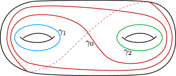
Figure 8.1. A Kleinian manifold whose limit set is the Apollonian gasket, homeomorphic to a genus two handlebody with parabolic locus marked

Let $\mathcal{E}=\{D_{j}\}$ be a collection of disjoint non-trivial compressing disks in $N$. Note that $\eta_{j}=\partial D_{j}$ forms a collection of disjoint simple closed curves on $\partial_{e}N$. The collection $\mathcal{E}$ is said to be maximal if cutting $N$ along all of $D_{j}$ produces a finite collection of topological balls $\{B_{k}\}$ and thickened tori $\{T_{l}\}$.

From now on we always assume $\mathcal{E}$ is maximal. After cutting along $\{D_{j}\}$, each $D_{j}$ becomes two disjoint disks $D_{j}^{+}$ and $D_{j}^{-}$. For each topological ball $B_{k}$, on its boundary lies the disjoint union of several of the disks $D_{j}^{\pm}$. Denote the portion of $\partial B_{k}$ coming from $\partial_{e}N$ by $\partial^{\prime}B_{k}$. For each thickened torus $T_{l}$, one of its boundary components contains one of the disks $D_{j}^{\pm}$. Denote the portion of the component from $\partial_{e}N$ by $\partial^{\prime}T_{l}$.

Since each $\gamma_{i}$ is homotopically nontrivial in $N$, it must intersect $\cup_{j}\eta_{j}$. Each segment of $\cup_{i}\gamma_{i}-\cup_{j}\eta_{j}$ lies on some $\partial^{\prime}B_{k}$ or $\partial^{\prime}T_{l}$, and connects two curves (possibly identical) among $\{\eta_{j}^{\pm}\}$, where $\eta_{j}^{\pm}=\partial D_{j}^{\pm}$. We have the following simple lemma.

Lemma 8.9.

The collection of curves $\{\gamma_{i}\}\cup\{\eta_{j}\}$ fills the surface $\partial_{e}N$, i.e. $\partial_{e}N-\cup_{i}\gamma_{i}-\cup_{j}\eta_{j}$ consists of disks.

Proof.

Suppose by contradiction that $\partial_{e}N-\cup_{i}\gamma_{i}-\cup_{j}\eta_{j}$ contains a nontrivial curve $\gamma$. Then in particular it lies on some $\partial^{\prime}B_{k}$ or some $\partial^{\prime}T_{l}$. In the former case, $\gamma$ is homotopically trivial in $N$, and in the latter case, it is homotopic to a curve on an interior toroidal boundary component. Moreover, since $\gamma$ does not intersect any $\gamma_{i}$, it is contained in a component $S^{\prime}$ of $\partial_{e}N-\cup_{i}\gamma_{i}$. But $S^{\prime}$ is incompressible in $N$, and no curve on $S^{\prime}$ represents a cuspidal curve around a rank-2 cusp. ∎

The collection $\mathcal{E}$ is called admissible if it is maximal, and satisfies the following conditions.

• For each segment of $\cup_{i}\gamma_{i}-\cup_{j}\eta_{j}$ contained in some $\partial^{\prime}B_{k}$, its endpoints do not lie on the same $\eta_{j}^{\pm}$.

• For each $B^{\prime}_{k}$, any path on $B^{\prime}_{k}$ connecting some $\eta_{j}^{\pm}$ to itself intersects some $\gamma_{i}\cap B_{k}^{\prime}$.

The following result reduces finding a subdivision rule to finding an admissible collection of compression disks.

Proposition 8.10.

Any admissible collection $\mathcal{E}$ of disjoint non-trivial compressing disks gives an irreducible simple finite or $\mathbb{Z}^{2}$-subdivision rule $\mathcal{R}$ on the graph $\mathcal{G}$ so that each face of the subdivision is a Jordan domain.

Remark.

We note that because of the arguments in §4.1, to obtain rigidity it is not necessary to make sure every face of the subdivision is a Jordan domain. Moreover, even though we have defined $\mathbb{Z}^{2}$-subdivisions with this additional assumption, it is easy to see that this is not necessary as well. However, the modification in §4.1 involves further subdivision, and in terms of the arguments below, this involves several copies of a fundamental domain. Here we instead give a geometrically meaningful modification so that the first level of subdivision can be described in a single fundamental domain.

Subdivisions and compressing disks

To give a precise statement and prepare the proof of Proposition 8.10, we first discuss how to translate the topological data of compressing disks to combinatorial information about subdivision of the graph $\mathcal{G}$.

Via the homeomorphism between the Kleinian manifold $(\overline{M},\partial\overline{M})$ and the compression body $(N,\partial N-P)$, objects discussed above (compressing disks, fragments of their boundary curves, etc.) are also present in $\overline{M}$, which we denote by the same notations.

In the universal cover $\mathbb{H}^{3}\cup\Omega$, choose lifts $\tilde{B}_{k}$ of each $B_{k}$ so that

• $\widetilde{B}_{k}$ is bounded by lifts $\widetilde{D}_{j}^{\pm}$ of compression disks;

• The boundary at infinity of each $\widetilde{D}_{j}^{\pm}$, denoted by $\widetilde{\eta}_{j}^{\pm}$, is a closed curve in $\hat{\mathbb{C}}$ whose only intersections with circles in $\mathcal{P}$ are points of tangency;

• The inward-pointing normals along each $\widetilde{D}_{j}^{\pm}$ points to a region $E_{j}^{\pm}$ bounded by $\widetilde{\eta}_{j}^{\pm}$, and $\bigcap_{D^{\pm}_{j}\text{ bounds }B_{k}}E_{j}^{\pm}$ is contained entirely in the domain of discontinuity – it is a lift of $\partial^{\prime}B_{k}-\cup_{i}\gamma_{i}$.

Note that each $\widetilde{\eta}_{j}^{\pm}$ determines a cycle $P_{j}^{\pm}$ in $\mathcal{G}$. We claim

Lemma 8.11.

If the collection $\mathcal{E}$ is admissible, then the cycles $P_{j}^{\pm}$ bounds a Jordan domain.

Proof.

If a cycle fails to bound a Jordan domain, then some vertices or edges are repeated. If an edge is repeated, the the corresponding curve $\widetilde{\eta}_{j}^{\pm}$ passes through a point of tangency twice. Since points of tangecy are parabolic fixed points, this only happens if $\eta_{j}^{\pm}$ is connected to itself by a segment of $\cup_{i}\gamma_{i}-\cup_{j}\eta_{j}$, contradicting admissibility. Technically, there might be several nested curves (which are orbits of some of $\widetilde{\eta}_{t}^{\pm}$ under the Kleinian group) passing through the same tangency twice (see Figure 8.2), but we can apply the argument above to the innermost curve.

Figure 8.2. Nested cycle repeating the same edge

Similarly, if some vertices (but none of the edges) are repeated, then there exist two distinct segments of $\widetilde{\eta}_{j}^{\pm}$ that lie in the same disk of the packing, and we can connect them via a path contained in the lift of the corresponding component of $\partial^{\prime}B_{k}-\cup_{i}\gamma_{i}$. This also contradicts admissibility. ∎

We now proceed to describe how to associate a subdivision rule to an admissible collection $\mathcal{E}$ of compressing disks. For simplicity, first assume that the Kleinian group $\Gamma$ contains no rank-2 parabolic subgroups. Then we can define a finite subdivsion rule $\mathcal{R}$ as follows.

The polygons.

The collection of polygons is $\{P_{j}^{\pm}\}$, where the interior of the polygon $P_{j}^{\pm}$ is chosen to be the part corresponding to the complement of $E_{j}^{\pm}$. Note that the complement of $P_{j}^{\pm}$ is naturally identified with $P_{j}^{\mp}$, since there exists an element $g_{j}^{\pm}\in\Gamma$ (possibly identity) mapping $E_{j}^{\mp}$ to the complement of $E_{j}^{\pm}$.

The subdivision.

For each $P_{j}^{\pm}$, let $B_{k}$ be the corresponding ball bounded by $D_{j}^{\mp}$ (note the change in the sign $+$ or $-$). Let $D_{j,t}^{\mp}$ denotes the other compressing disks bounding $B_{k}$. Then the corresponding curves $\widetilde{\eta}_{j,t}^{\mp}$ lie in the domain $E_{j}^{\mp}$. In particular, they determine polygons $P_{j,t}^{\mp}$ in $\mathcal{G}$ contained in the complement of $P_{j}^{\mp}$. Since $E_{j}^{\mp}\bigcap\cap_{t}E_{j,t}^{\mp}$ is contained entirely in the domain of discontinuity, we conclude that

$$\overline{(P_{j}^{\mp})^{c}}=\bigcup_{t}P_{j,t}^{\mp}.$$

The map $g_{j}^{\pm}$ induces a cellular map from $\overline{(P_{j}^{\mp})^{c}}$ to $P_{j}^{\pm}$, and hence also a subdivision of $P_{j}^{\pm}$.

The cellular maps.

For the subdivision $P_{j}^{\pm}=\bigcup_{t}g_{j}^{\pm}(P_{j,t}^{\mp})$, the inverse of $g_{j}^{\pm}$ identifies each piece to one of the original polygons.

The $\mathcal{R}$-complex

It remains to check that we can construct an $\mathcal{R}$-complex $X$ homeomorphic to the sphere so that the corresponding spherical subdivision graph is precisely $\mathcal{G}$. This is straightforward: choose any $j$. Then the polygon $P_{j}^{+}$ and its complement gives the sphere the structure of an $\mathcal{R}$-complex, as $(P_{j}^{+})^{c}$ is identified with $P_{j}^{-}$. Note that orbits of $\cup_{k}\tilde{B}_{k}$ under $\Gamma$ tile $\mathbb{H}^{3}$. For each $n$, subdividing $\mathcal{R}^{n}(X)$ is tantamount to moving into a new piece in this tiling. Since the cellular maps identify each piece in the subdivision with the original polygons via an element of $\Gamma$, the subdivision graph we obtain is precisely $\mathcal{G}$.

Rank-2 cusps.

We briefly discuss the case where $\Gamma$ contains at least one rank-2 parabolic subgroup. Without loss of generality, suppose $D_{1}^{+}$ bounds a thickened torus $T_{1}$. Correspondingly, $D_{1}^{-}$ bounds a ball, and its lift $\widetilde{D}_{1}^{-}$ is bounded at infinity by $\widetilde{\eta}_{1}^{-}$, with the corresponding domain $E_{1}^{-}$. Suppose the parabolic fixed point is at infinity. Then the action of the rank-2 parabolic subgroup gives $\mathbb{Z}^{2}$-orbits of $\widetilde{\eta}_{1}^{-}$.

Note that the cycle determined by $\widetilde{\eta}_{1}^{-}$ bounds a Jordan domain. The boundary of the polygons $P_{1}^{\pm}$ are both this cycle, and the interior $P_{1}^{+}$ is chosen to be the component not containing $\infty$, while the interior of $P_{1}^{-}$ is chosen to be the complement. As $\mathbb{C}-\bigcup_{g\in\mathbb{Z}^{2}}g\cdot E_{1}^{-}$ is contained entirely in the domain of discontinuity, the $\mathbb{Z}^{2}$-orbit of $P_{1}^{+}$ gives a $\mathbb{Z}^{2}$-tiling. Using the notation of §7, we set $Q_{1}^{+}=P_{1}^{-}$. Note that clearly

$$Q_{1}^{+}=\overline{\bigcup_{g\in\mathbb{Z}^{2}-id}g\cdot P_{1}^{+}}.$$

Now suppose $P_{1}^{+},Q_{1}^{+},\ldots,P_{s}^{+},Q_{s}^{+}$ are all the polygons obtained as above for each thickened torus $T_{l}$, and $P_{m+1}^{\pm},\ldots,P_{t}^{\pm}$ the remaining polygons obtained from other compressing disks, then one can define subdivisions of each polygon similarly as above. This gives a $\mathbb{Z}^{2}$-subdivision rule, as desired.

Construction of admissible $\mathcal{E}$

It remains to explicitly choose an admissible collection $\mathcal{E}$ of compressing disks on $N$. Suppose $\partial_{e}N$ is a surface of genus $g$, and there are $s$ toroidal boundary components (clearly $s\leq g$).

It is easy to see that we can find $g$ nontrivial compressing disks $D_{1},\ldots,D_{g}$ (with boundary $\eta_{1},\ldots,\eta_{g}$), so that $D^{+}_{l}$ bounds thickened tori $T_{l}$ for $1\leq l\leq s$, and $N-\bigcup_{l=1}^{s}T_{l}-\bigcup_{j=s+1}^{g}D_{j}$ is a connected ball $B_{1}$. (The only exception is $g=2$ and $s=2$, where we only need one compressing disk $D_{1}$ to decompose $N$ into two thickened tori.) If the collection $\mathcal{E}:=\{D_{1},\ldots,D_{s}\}$ is already admissible, then we are done. Otherwise, we can modify the collection as follows.

First consider $D_{1}$; the other disks bounding tori can be modified similarly. First suppose on $B_{1}$, there is a segment $L$ of $\cup\gamma_{i}-\cup_{j}\eta_{j}$ on $B_{1}$ connecting $\eta_{1}$ to itself. The end points of $L$ divides $\eta_{1}$ into two parts $\eta_{1}^{\prime}$ and $\eta_{1}^{\prime\prime}$. We first claim

Lemma 8.12.

There exists a segment $L^{\prime}$ of $\cup\gamma_{i}-\cup_{j}\eta_{j}$ on $\partial^{\prime}T_{1}$ connecting the interior of $\eta_{1}^{\prime}$ to that of $\eta_{1}^{\prime\prime}$.

Proof.

We can connect the two endpoints of $L$ in $\partial^{\prime}T_{1}$ via a simple segment $J$ not homotopic to either $\eta_{1}^{\prime}$ nor $\eta_{1}^{\prime\prime}$. Then $L\cup J$ is homotopic in $N$ to a simple close curve on the torus boundary. On the other hand, if $J$ does not intersect any $\gamma_{i}$, the curve $L\cup J$ can be homotoped in $\partial_{e}N$ to be disjoint from $\cup\gamma_{i}$. But such a curve cannot be homotopic to a cuspidal curve around the rank-2 cusp, a contradiction. So $J$ must intersect some segment $L^{\prime}$ of $\gamma_{i}$ in $\partial^{\prime}T_{1}$, and it is then easy to see that $L^{\prime}$ connects $\eta_{1}^{\prime}$ to $\eta_{1}^{\prime\prime}$. ∎

Figure 8.3. Modifying the disk bounding a thickened torus. To avoid crowding the figure, the torus interior boundary component is not drawn.

Now as in Figure 8.3, tracing two parallel copies of $L$, one copy of $\eta_{1}$, and two parallel copies of $L^{\prime}$, we obtain a curve $\eta_{1}^{\prime}$ and it is easy to see that it bounds a compressing disk $D_{1}^{\prime}$. Clearly there are fewer segments of $\cup_{i}\gamma_{i}-\cup_{j}\eta_{j}$ connecting $\eta_{1}^{\prime}$ to itself, and this does not affect the disks bounding other thickened tori. Inductively, we can thus modify $D_{1},\ldots,D_{s}$ so that no segment of $\cup_{i}\gamma_{i}-\cup_{j}\eta_{j}$ connects $\eta_{j}^{-}$ to itself for $1\leq j\leq s$. An entirely analogous argument also ensures that the second condition in the definition of admissibility is satisfied for these disks.

Next we consider $D_{g}$ assuming it does not bounds a thickened torus. Suppose there is a segment $L$ of $\cup_{i}\gamma_{i}-\cup_{j}\eta_{j}$ connecting $D_{g}^{+}$ to itself in $B_{1}$. Tracing two parallel copies of $L$ and a copy of $\eta_{g}$, we obtain two compressing disks $D_{g}^{1}$ and $D_{g}^{2}$; see Figure 8.4.

Figure 8.4. Modifying a disk not bounding a thickened torus

Replacing $D_{g}$ with $D_{g}^{1}$ and $D_{g}^{2}$, note that the number of segments violating the first condition in admissibility either reduces by 1, or remain the same, if the two segments in $\cup_{i}\gamma_{-}\cup_{j}\eta_{j}$ extending $L$ beyond its two endpoints terminate at the same $\eta_{j}^{\pm}$. We can then replace $D_{j}$ similarly by two disks $D_{j}^{1}$ and $D_{j}^{2}$. This process can be repeated, and terminates when one of the following happens:

• The two endpoints of extended $L$ are connected by some segment of $\cup_{k}\gamma_{k}-\cup_{j}\eta_{j}$. This is impossible since we now have a curve among $\gamma_{i}$ that is homotopically trivial.

• The two segments extending $L$ terminate at two different $\eta_{j}^{\pm}$. In this case, the number of segments violating the first condition in admissibility decreases by 1.

• The two endpoints of $L$ lie on some $\eta_{j}$ bounding a thickened torus. In this case, modify the disk as in Figure 8.3, we again reduce the number of segments violating the first condition by 1.

Inductively, we can thus guarantee the first condition is satisfied. An entirely analogous argument also guarantees the second condition is satisfied.

In this way, we obtain an admissible collection of compressing disks, as desired.

A topological model

We give a purely topological way of visualizing the subdivision rule. For simplicity, we focus on one simple example given in Figure 8.1.

It is easy to find an admissible collection of compressing disks. In fact, for one such collection, after cutting the handlebody along the disks, we obtain a topological ball $B$ as in Figure 5(a). The subdivisions are also illustrated on the Apollonian circle packing in Figure 5(b).

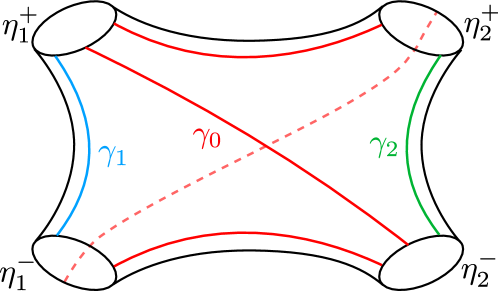
(a)

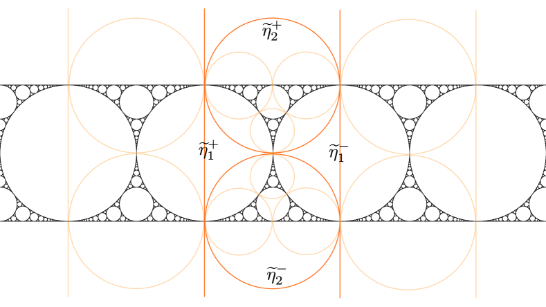
(b)

Figure 8.5. Cutting along an admissible collection of compressing disks, topologically (A) or on the limit set (B)

We can also use $B$ as a fundamental domain to build up a universal cover for the handlebody, which is homotopic to a infinite 4-valent tree (note that $\gamma_{1}$ and $\gamma_{2}$ generates the fundamental group); see Figure 8.6.

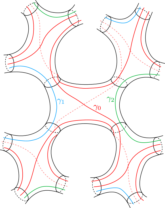
Figure 8.6. An infinite tree model for the universal cover

In this picture, the parabolic locus is unraveled to be a collection of infinite lines. Each component of the complement of these lines on the boundary corresponds to a disk in the packing. Entering a new copy of the ball $B$ is tantamount to entering a piece of the subdivision at the next level. The end space of the tree is naturally identified with the limit set with each parabolic fixed point blown up to be two points, which are also the ends of the line associated to the corresponding parabolic element.

8.4. Further remarks

With non-toroidal interior boundary components

When $N$ has at least one non-toroidal interior boundary component, and is not homoemorphic to $\partial_{e}N\times[0,1]$, we can still cut off each interior boundary component with a compressing disk. However, it might not be possible to modify these disks so that the corresponding cycles in the nerve $\mathcal{G}$ bounds a Jordan domain.

Moreover, choose a compressing disk $D$ so that cutting $N$ along $D$ produces a component homeomorphic to the trivial interval bundle over a non-toroidal interior boundary component, and let $P$ be the polygon in $\mathcal{G}$ bounded by the cycle determined by $D$. Then $\mathcal{G}-\bigcup_{\gamma\in\Gamma}\gamma\cdot P$ contains no loops, due to a similar argument as the tree case.

Topology from the nerve, revisited

We come back to the question of extracting topological information about the 3-manifold from the nerve. We have the converse to the construction above:

Proposition 8.13.

If $\mathcal{G}$ is a spherical subdivision graph for a finite subdivision rule, then $N$ is a handlebody. Similarly, if $\mathcal{G}$ is a spherical subdivision graph for a $\mathbb{Z}^{2}$-subdivision rule, then the interior boundary of $N$ consists of tori.

Proof.

We have the topology of $N$ has one of the types (1)-(4) listed just above Proposition 8.8. When $N$ is not a handlebody, say of type (2), then the corresponding Kleinian group has a rank-2 parabolic subgroup. Smaller and smaller polygons containing the corresponding parabolic fixed point has more and more sides, so no finite subdivision rule exists. Similar arguments can be made for all other cases.

Suppose now $\mathcal{G}$ is a spherical subdivision graph for a $\mathbb{Z}^{2}$-subdivision rule. Then we have a $\mathbb{Z}^{2}$-action on $\mathcal{G}$ coming from the subdivision rule. If $N$ is a handlebody, by combinatorial rigidity in this case the $\mathbb{Z}^{2}$-action realizes as Möbius maps fixing the circle packing. But this is only possible with rank-2 cusps.

On the other hand, clearly $\mathcal{G}$ cannot be a tree. Finally, if $N$ is of type (4), the limit set of any subgroup $\Gamma^{\prime}$ of $\Gamma$ corresponding to a geometrically infinite end is surrounded by cycles of disks in the packing. The length of the cycle grows exponentially as we approach the limit set (since $\Gamma^{\prime}$ contains free groups); but this means $\mathcal{G}$ does not come from a $\mathbb{Z}^{2}$-subdivision rule, since the length of the cycles can only grow linearly in that case. ∎

References

- [Ago04] I. Agol. Tameness of hyperbolic 3-manifolds. arXiv:math/0405568, 2004.
- [AL11] A. Avila and M. Lyubich. The full renormalization horseshoe for unimodal maps of higher degree: exponential contraction along hybrid classes. Publ. Math. IHES, 114: 171–223, 2011
- [AL22] A. Avila and M. Lyubich. Lebesgue measure of Feigenbaum Julia sets. Ann. of Math. (2), 195: 1–88, 2022
- [BO22] Y. Benoist and H. Oh. Geodesic planes in geometrically finite acylindrical manifolds. Ergodic Theory Dynam. Systems, 42: 514–553, 2022.
- [BJM13] I. Biringer, J. Johnson and Y. Minksy. Extending pseudo-Anosov maps into compression bodies. J. Topol., 6: 1019–1042, 2013.
- [BKK22] N. Bogachev, A. Kolpakov and A. Kontorovich. Kleinian sphere packings, reflection groups, and arithmeticity. arXiv:2203.01973, 2022.
- [BKM09] M. Bonk, B. Kleiner and S. Merenkov. Rigidity of Schottky sets. Amer. J. Math., 131(2):409–443, 2009.
- [BM13] M. Bonk and S. Merenkov. Quasisymmetric rigidity of square Sierpiński carpets. Ann. of Math. (2), 177(2):591–643, 2013.
- [BF11] J. Bourgain and E. Fuchs. A proof of the positive density conjecture for integer Apollonian circle packings. J. Amer. Math. Soc., 24(4): 945–967, 2011.
- [BK14] J. Bourgain and A. Kontorovich. On the local-global conjecture for integral Apollonian gaskets. Invent. Math., 196(3): 589–650, 2014.
- [BLM16] M. Bonk, M. Lyubich and S. Merenkov. Quasisymmetries of Sierpiński carpet Julia sets. Adv. Math., 301: 383–422, 2016.
- [Bon11] M. Bonk. Uniformization of Sierpiński carpets in the plane. Invent. Math., 186:559–665, 2011.
- [BS97] P. Bowers and K. Stephenson. A “regular” pentagonal tiling of the plane. Conform. Geom. Dyn., 1:58–68, 1997.
- [BS17] P. Bowers and K. Stephenson. Conformal tilings I: foundations, theory, and practice. Conform. Geom. Dyn., 21:1–63, 2017.
- [Bro85] R. Brooks. On the deformation theory of classical Schottky groups. Duke Math. J., 4:1009–1024, 1985.
- [Bro86] R. Brooks. Circle packings and co-compact extensions of Kleinian groups. Invent. Math., 86:461–469, 1986.
- [CG06] D. Calegari and D. Gabai. Shrinkwrapping and the taming of hyperbolic 3-manifolds. J. Amer. Math. Soc., 19(2): 385–446, 2006.
- [CFKP03] J. Cannon, W. Floyd, R. Kenyon and W. Parry. Constructing rational maps from subdivision rules. Conform. Geom. Dyn., 7:76–102, 2003.
- [CFP01] J. Cannon, W. Floyd and W. Parry. Finite subdivision rules. Conform. Geom. Dyn., 5:153–196, 2001.
- [CFP06a] J. Cannon, W. Floyd and W. Parry. Expansion complexes for finite subdivision rules. I. Conform. Geom. Dyn., 10:63–99, 2006.
- [CFP06b] J. Cannon, W. Floyd and W. Parry. Expansion complexes for finite subdivision rules. II. Conform. Geom. Dyn., 10:326–354, 2006.
- [CFP07] J. Cannon, W. Floyd and W. Parry. Constructing subdivision rules from rational maps. Conform. Geom. Dyn., 11:128–136, 2007.
- [CFPP09] J. Cannon, W. Floyd, W. Parry and K. Pilgrim. Subdivision rules and virtual endomorphisms. Geom. Dedicata, 141:181–195, 2009.
- [COK17] C. Collins, G. Orick, and K. Stephenson. A linearized circle packing algorithm. Computational Geometry: Theory and Applications, 64:13–19, 2017.
- [DH85] A. Douady and J. Hubbard. On the dynamics of polynomial-like maps. Ann. Sc. Éc. Norm. Sup., 18:287–343, 1985.
- [DH93] A. Douady and J. Hubbard. A proof of Thurston’s topological characterization of rational functions. Acta Math., 171(2):263–297, 1993.
- [DLS20] D. Dudko, M. Lyubich, and N. Selinger. Pacman renormalization and self-similarity of the Man- delbrot set near Siegel parameters. J. Amer. Math. Soc., 33: 653–733, 2020.
- [GLMWY03] R. Graham, J. Lagarias, C. Mallows, A. Wilks and C. Yan. Apollonian circle packings: number theory. J. Number Theory, 100: 1–45, 2003.
- [GLMWY05] R. Graham, J. Lagarias, C. Mallows, A. Wilks and C. Yan. Apollonian circle packings: geometry and group theory I. the Apollonian group. Discrete Comput. Geom., 34: 547–585, 2005.
- [He91] Z-X. He. An estimate for hexagonal circle packings. J. Differential Geom., 33(2):395–412, 1991.
- [HL10] Z-X. He and J. Liu. A sharp estimate for the hexagonal circle packing constants. Geom. Dedicata, 146:193–210, 2010.
- [HR93] Z-X. He and B. Rodin. Convergence of circle packings of finite valence to Riemann mappings.. Comm. Anal. Geom., 1(1):31–41, 1993.
- [HS93] Z-X. He and O. Schramm. Fixed points, Koebe uniformization and circle packings. Ann. of Math. (2), 137(2):369–406, 1993.
- [HS94] Z-X. He and O. Schramm. Rigidity of circle domains whose boundary has -finite linear measure. Invent. Math., 115:297–310, 1994.
- [HS96] Z-X. He and O. Schramm. On the convergence of circle packings to the Riemann map. Invent. Math., 125:285–305, 1996.
- [HS98] Z-X. He and O. Schramm. The -convergence of hexagonal disk packings to the Riemann map. Acta Math., 180(2):219–245, 1998.
- [Hem79] J. Hempel. The Poincaré metric on the twice punctured plane and the theorems of Landau and Schottky. J. London Math. Soc., 20:435–445, 1979.
- [IS08] H. Inou and M. Shishikura. The renormalization for parabolic fixed points and their perturbations. Manuscript., 2008.
- [KK21] M. Kapovich and A. Kontorovich. On superintegral Kleinian sphere packings, gugs, and arithmetic groups. arXiv:2104.13838, 2021.
- [Ken10] A. Kent. Skinning maps. Duke Math. J., 151:279–336, 2010.
- [KMT03] S. Kojima, S. Mizushima and S. P. Tan. Circle packings on surfaces with projective structures. J. Differential Geom., 63(3): 349–397, 2003.
- [KMT06] S. Kojima, S. Mizushima and S. P. Tan. Circle packings on surfaces with projective structures and uniformization. Pacific J. Math., 225(2): 287–300, 2006.
- [KN19] A. Kontorovich and K. Nakamura. Geometry and arithmetic of crystallographic sphere packings. Proc. Nat. Acad. Sci., 116(2): 436–441, 2019.
- [KO11] A. Kontorovich and H. Oh. Apollonian circle packings and closed horospheres on hyperbolic 3-manifolds. J. Amer. Math. Soc., 24: 603–648, 2011.
- [LLM22] R. Lodge, Y. Luo, and S. Mukherjee. Circle packings, kissing reflection groups and critically fixed anti-rational maps. Forum Math. Sigma, vol. 10, paper no. e3, 2022.
- [LLMM23] R. Lodge, M. Lyubich, S. Merenkov, and S. Mukherjee. On dynamical gaskets generated by rational maps, Kleinian groups, and Schwarz reflections. Conform. Geom. Dyn., 27(1): 1–54, 2023.
- [Lyu99] M. Lyubich. Feigenbaum-Coullet-Tresser Universality and Milnor’s Hairiness Conjecture. Ann. of Math. (2), 149(2): 319–420, 1999.
- [LZ23] Y. Luo, and Y. Zhang. On quasiconformal non-equivalence of gasket Julia sets and limit sets. Preprint, 2023.
- [Mas74] B. Maskit. Intersections of component subgroups of Kleinian groups. In L. Greenberg, editor, Discontinuous Groups and Riemann Surfaces: Proceedings of the 1973 Conference at the University of Maryland, 349–367. Ann. Math. St. 79, Princeton University Press, 1974.
- [McM90] C. McMullen. Iteration on Teichmüller space. Invent. Math., 99(2):425–454, 1990.
- [McM94] C. McMullen. Complex Dynamics and Renormalization (AM-135). Princeton University Press, 1994.
- [McM96] C. McMullen. Renormalization and 3-Manifolds which fiber over the circle (AM-142). Princeton University Press, 1996.
- [McM98] C. McMullen. Self-similarity of Siegel disks and Hausdorff dimension of Julia sets. Acta Math., 180:247–292, 1998.
- [Mer12] S. Merenkov. Planar relative Schottky sets and quasisymmetric maps. Proc. Lond. Math. Soc. (3), 104(3):455–485, 2012.
- [Mer14] S. Merenkov. Local rigidity of Schottky maps. Proc. Lond. Math. Soc. (3), 142(12):4321–4332, 2014.
- [NS12] H. Namazi and J. Souto Non-realizability and ending laminations: Proof of the density conjecture. Acta Math., 209(2):323-395, 2012.
- [OS12] H. Oh and N. Shah. The asymptotic distribution of circles in the orbits of Kleinian groups. Invent. Math., 187: 1–35, 2012.
- [Ota88] J.-P. Otal. Courants géodésiques et surfaces. PhD Thesis, Universit’e de Paris-Sud, Orsay, 1988.
- [QYZ19] W. Qiu, F. Yang and J. Zeng. Quasisymmetric geometry of Sierpiński carpet Julia sets. Fund. Math., 244: 73–107, 2019.
- [RS87] B. Rodin and D. Sullivan. The convergence of circle packings to the Riemann mapping. J. Differential Geom., 26(2):349–360, 1987.
- [Sch91] O. Schramm. Rigidity of infinite (circle) packings. J. Amer. Math. Soc., 4(1):127–149, 1991.
- [Sel11] N. Selinger. Thurston’s pullback map on the augmented Teichmüller space and applications. Invent. Math., 189:111–142, 2011.
- [Ste03] K. Stephenson. Circle packing: a mathematical tale. Notices Amer. Math. Soc., 11:1376–1388, 2003.
- [Sul81] D. Sullivan. On the ergodic theory at infinity of an arbitrary discrete group of hyperbolic motions. In I. Kra and B. Maskit, editors, Riemann Surfaces and Related Topics: Proceedings of the 1978 Stony Brook Conference, 465-496. Ann. Math. St. 97, Princeton University Press, 1981.
- [Thu82] W. Thurston. Hyperbolic geometry and 3-manifolds In Low-dimensional topology (Bangor, 1979), 9–25. London Math. Soc. Lecture Note Ser. 48, Cambridge Univ. Press, 1982.
- [Thu86] W. Thurston. Hyperbolic structures on 3-manifolds I: Deformation of acylindrical manifolds. Ann. of Math., 124: 203–246, 1986.
- [Thu88] W. Thurston. On the geometry and dynamics of diffeomorphisms of surfaces. Bull. Am. Math. Soc., 19(2): 417–431, 1988.
- [Zha22] Y. Zhang. Elementary planes in the Apollonian orbifold. Trans. Amer. Math. Soc., 376(1):453–506, 2023.