Understanding Turbo Codes: A Signal Processing Study

Abstract

In this paper, we study turbo codes from the digital signal processing point of view by defining turbo codes over the complex field. It is known that iterative decoding and interleaving between concatenated parallel codes are two key elements that make turbo codes perform significantly better than the conventional error control codes. This is analytically illustrated in this paper by showing that the decoded noise mean power in the iterative decoding decreases when the number of iterations increases, as long as the interleaving decorrelates the noise after each iterative decoding step. An analytic decreasing rate and the limit of the decoded noise mean power are given. The limit of the decoded noise mean power of the iterative decoding of a turbo code with two parallel codes with their rates less than $1/2$ is one third of the noise power before the decoding, which can not be achieved by any non-turbo codes with the same rate. From this study, the role of designing a good interleaver can also be clearly seen.

1 Introduction

Turbo codes have recently received considerable attentions, see for example [1-9], due to the near Shannon limit performance. The recent research results [2] on turbo codes have indicated that the bit error rate (BER) can reach $10^{-5}$ at signal-to-noise ratio (SNR) $E_{b}/N_{0}=0.0$dB. This “magic” performance has been surprising the communication community lately, and meanwhile questions, doubts, and explanations have been followed up too. The main question is: what is the magic of turbo codes? In turbo codes, there are two key elements: iterative decoding and interleaving between concatenated parallel codes. A simple example of rate 1/2 turbo code is shown in Fig. 1(a) for encoding and Fig. 1(b) for decoding, where $\downarrow 2$ means downsampling by $2$ , i.e., taking one in each two samples, and $z^{-1}$ denotes the delay variable as denoted by $D$ in the channel coding literature. An intuitive explanation for the super performance of turbo codes is the following.

Because of the hardware limitations, the error correction capability in low SNR environments is limited due to the limited distance property of a limited size error correction code. This means that implementing a decoding algorithm once may not be able to correct all errors but some errors, i.e., the total number of errors is reduced. A natural question is, to correct more errors, why one does not implement the decoding algorithm for the decoded signal again. To answer this question, one should notice that, although the total number of errors after the first decoding is reduced, the decoding algorithm may cause patterned errors, such as burst errors. These patterned errors may increase the number of total errors of the second implementation of the decoding algorithm. This implies that the direct implementation of cascaded multiple decoding algorithms may not be helpful. To get around of the patterned errors, an intuitive method is to add an interleaver between two cascaded decoding algorithms to spread the patterned errors over a long period of time. The interleaving between two decoders forces the interleaving between the concatenated encoders.

Figure 1: A rate 1/2 turbo code.

Although the above intuitive explanation is sometimes good enough, a quantitative analysis is more important to understand turbo codes better. There have been several excellent articles in the literature on the performance analysis of turbo codes, such as [3-9]. A strong analytic analysis is still needed to show the better performance of turbo codes than the conventional codes. Most recently, Forney in [18] mentioned “turbo codes work very well, but we don’t understand them.” The goal of this paper is to study turbo codes from the digital signal processing perspective by extending turbo codes and other codes defined from finite fields to the the complex field, and comparing them on the complex field. Since all codes here are defined over the complex field, the maximal likelihood decoding is the least squared error decoding, which can be achieved by solving a system of linear equations. By doing so, we show that the decoded noise mean power decreases when the iteration number in the decoding increases under the condition that the interleaving between concatenated parallel codes decorrelates the noise after each decoding iteration. Given a rate of a turbo code, the decreasing rate of the decoded noise mean power in terms of the number of iterations in the decoding is given, and the limit of the decoded noise mean power is also given when the number of iterations tends to infinity. It turns out that the decoded noise mean power in the limit sense can not be achieved by any non-iterative codes, i.e., non-turbo codes, with the same rate.

This paper is organized as follows. In Section 2, we study a general systematic error control code defined on the complex field and formulate the noise power after the least squared error decoding. The study in this section provides a foundation for the late analysis. In Section 3, we study the decoded noise mean power after the iterative turbo code decoding. In Section 4, we present some numerical examples.

2 Linear Error Control Codes Over the Complex Field

To study turbo codes defined on the complex field, in this section we first study a general linear error control code defined over the complex field, which have been recently discussed in [10]. As mentioned in [10], there are two advantages of error control codes defined on the complex field over the conventional error control codes. Since error control codes are defined on the complex field, all arithmetics are in the complex field and therefore the maximal likelihood decoding is the least squared error solution, that is the solution of a linear system. This is the first advantage, i.e., linear algorithm decoding. Since all channel distortions are with the complex field arithmetic, error control codes over the complex field can be designed to completely cancel an FIR intersymbol interference (ISI), which is not possible for any error control codes defined on finite fields. In [11-13], channel independent error control codes are designed to cancel the ISI, which are called ambiguity resistant codes. This is the second advantage.

In this section, we focus on channels with only additive random noise and study the noise power change after the least squared error decoding.

A linear error control code defined on the complex field is usually represented by

$$Y(z)=G(z)X(z),$$ (2.1)

where $X(z)=\sum_{n}X(n)z^{-n}$, $G(z)=\sum_{n=0}^{Q_{G}}G(n)z^{-n}$, and $Y(z)=\sum_{n}Y(n)z^{-n}$ are the $z$-transform of $K\times 1$ input vector sequence $X(n)$, $N\times K$ code generator matrix with order $Q_{G}$, and the $z$-transform of $N\times 1$ output vector sequence $Y(n)$, respectively. In particular, for a rate $K/N$ block linear error control code,

$$Y=GX,$$ (2.2)

where $X$, $Y$ and $G$ are $K\times 1$, $N\times 1$ and $N\times K$ (vectors) matrices, respectively. On the other hand, a convolutional code in (2.1) can also be represented by the block representation (2.2), where $G$ is the generalized Sylvester matrix of $G(z)$:

$$\left[\begin{array}[]{ccccc}G(Q_{G})&\cdots&G(0)&\cdots&0\\ \vdots&\ddots&\ddots&\ddots&\vdots\\ 0&\cdots&G(Q_{G})&\cdots&G(0)\end{array}\right].$$ (2.3)

Because of the mutual representations of block and convolutional codes in (2.1)-(2.3), without loss of generality, we focus on the block representation (2.2). A systematic rate $K/N$ block code $G$ is

$$G=\left[\begin{array}[]{c}I_{K}\\ F\end{array}\right],$$ (2.4)

where $I_{K}$ is the $K\times K$ identity matrix and $F$ is an $(N-K)\times K$ constant matrix. Since, in turbo codes, systematic codes are usually used, in the rest of this section we focus on systematic block codes. Let $G$ in (2.4) be

$$G=\left[\begin{array}[]{c}I_{K}\\ F\end{array}\right]=\left[\begin{array}[]{cccc}1&0&\cdots&0\\ 0&1&\cdots&0\\ \vdots&\vdots&\vdots&\vdots\\ 0&0&\cdots&1\\ g_{K+1,1}&g_{K+1,2}&\cdots&g_{K+1,K}\\ \vdots&\vdots&\vdots&\vdots\\ g_{N,1}&g_{N,2}&\cdots&g_{N,K}\end{array}\right].$$ (2.5)

To preserve the code output signal power, i.e., the output signal power is equal to the input signal power, the following normalization on $G$ is imposed:

$$\sum_{k=1}^{K}|g_{n,k}|^{2}=1,\,\,K+1\leq n\leq N.$$ (2.6)

The received signal is

$$\tilde{Y}=GX+\eta,$$ (2.7)

where $X=(X(1),\cdots,X(K))^{T}$, $\tilde{Y}=(\tilde{Y}(1),\cdots,\tilde{Y}(N))^{T}$, $\eta=(\eta(1),\cdots,\eta(N))^{T}$ are the input signal, the received signal and the additive random noise, respectively, and ^T means the transpose. The additive noise $\eta(n)$ is assumed i.i.d. and with mean $0$ and variance (or power) $\sigma_{\eta}^{2}$.

The maximal likelihood decoding of (2.7) is the least squared error solution:

$$\hat{X}=(G^{\dagger}G)^{-1}G^{\dagger}\tilde{Y}=X+(G^{\dagger}G)^{-1}G^{\dagger}\eta,$$ (2.8)

where ^† means the transpose conjugate. Thus, the noise after the decoding is

$$\hat{\eta}=(G^{\dagger}G)^{-1}G^{\dagger}\eta,$$ (2.9)

where $\eta$ is the additive noise before decoding and has power $\sigma_{\eta}^{2}$. We next want to calculate the mean power of this decoded noise $\hat{\eta}$.

Let $\eta=(\eta_{1}^{T},\eta_{2}^{T})^{T}$. Then $\eta_{1}$ and $\eta_{2}$ are independent each other. It is not hard to see that

$$\hat{\eta}=(I_{K}+F^{\dagger}F)^{-1}(\eta_{1}+F^{\dagger}\eta_{2}).$$ (2.10)

Let the singular value decomposition of $F$ be

$$F=U\Lambda V,$$ (2.11)

where $U=(u_{k,l})$ and $V=(v_{m,n})$ are $N\times N$ and $K\times K$ unitary matrices, respectively, and $\Lambda$ is the diagonal matrix. There are two cases for the diagonal matrix $\Lambda$.

Case I: $N-K<K$.

In this case,

$$\Lambda=\left[\mbox{diag}(\alpha_{1},\cdots,\alpha_{N-K}),0_{(N-K)\times(2K-N)}\right],$$ (2.12)

where $\alpha_{1}$, …, $\alpha_{N-K}$ with $|\alpha_{1}|\geq\cdots\geq|\alpha_{N-K}|$ are the singular values of $F$. Then (2.10) becomes

$$\hat{\eta}=V^{\dagger}\mbox{diag}\left(\frac{1}{1+|\alpha_{1}|^{2}},\cdots,\frac{1}{1+|\alpha_{N-K}|^{2}},1,\cdots,1\right)(V\eta_{1}+\Lambda^{\dagger}U^{\dagger}\eta_{2}).$$

Let $\hat{\eta}=(\hat{\eta}(1),\cdots,\hat{\eta}(K))^{T}$, then, by some algebra, the power of the $k$th component $\hat{\eta}(k)$ of $\hat{\eta}$ is

$$\sigma_{\hat{\eta}(k)}^{2}=\sigma_{\eta_{1}}^{2}\left(\sum_{m=1}^{N-K}|v_{m,k}|^{2}\frac{1}{(1+|\alpha_{m}|^{2})^{2}}+\sum_{m=N-K+1}^{K}|v_{m,k}|^{2}\right)+\sigma_{\eta_{2}}^{2}\sum_{m=1}^{N-K}|v_{m,k}|^{2}\frac{|\alpha_{m}|^{2}}{(1+|\alpha_{m}|^{2})^{2}},$$ (2.13)

where $v_{m,k}$ are the entries of the unitary matrix $V$ and $\sigma_{\eta_{i}}^{2}$ is the power of $\eta_{i}$ for $i=1,2$, which are equal to $\sigma_{\eta}^{2}$. Therefore, by the unitariness of the matrix $V$, the mean power of the decoded noise $\hat{\eta}$ is

$$\sigma_{\hat{\eta}}^{2}=\frac{\sigma_{\eta_{1}}^{2}}{K}\left(\sum_{k=1}^{N-K}\frac{1}{(1+|\alpha_{k}|^{2})^{2}}+2K-N\right)+\frac{\sigma_{\eta_{2}}^{2}}{K}\sum_{k=1}^{N-K}\frac{|\alpha_{k}|^{2}}{(1+|\alpha_{k}|^{2})^{2}}.$$ (2.14)

Since $\sigma_{\eta_{1}}^{2}=\sigma_{\eta_{2}}^{2}=\sigma_{\eta}^{2}$,

$$\sigma_{\hat{\eta}}^{2}=\frac{\sigma_{\eta}^{2}}{K}\left(\sum_{k=1}^{N-K}\frac{1}{1+|\alpha_{k}|^{2}}+2K-N\right).$$ (2.15)

By the normalization (2.6),

$$\sum_{k=1}^{K}|\alpha_{k}|^{2}=\sum_{n=K+1}^{N}\sum_{k=1}^{K}|g_{n,k}|^{2}=N-K,$$ (2.16)

where $\alpha_{N-K+1}=\cdots=\alpha_{K}=0$.

Given a rate $K/N$, by (2.16) the above mean power $\sigma_{\hat{\eta}}^{2}$ in (2.15) reaches the minimum when and only when $|\alpha_{k}|=1$ for $1\leq k\leq N-K$ and the minimum is

$$\sigma_{\hat{\eta}}^{2}=\frac{\sigma_{\eta}^{2}}{K}\left(\frac{N-K}{2}+2K-N\right)=\left(1-\frac{N-K}{2K}\right)\sigma_{\eta}^{2}.$$ (2.17)

In this case, the above minimum mean power can be expressed in terms of the powers $\sigma_{\eta_{i}}^{2}$ for $i=1,2$ as

$$\sigma_{\hat{\eta}}^{2}=\frac{7K-3N}{4K}\sigma_{\eta_{1}}^{2}+\frac{N-K}{4K}\sigma_{\eta_{2}}^{2}.$$ (2.18)

This formula will be used in Section 3 later.

Case II: $N-K\geq K$.

In this case,

$$\Lambda=\left[\begin{array}[]{c}\mbox{diag}(\alpha_{1},\cdots,\alpha_{K})\\ 0_{(N-K)\times K}\end{array}\right],$$ (2.19)

where $\alpha_{1}$, …, $\alpha_{K}$ with $|\alpha_{1}|\geq\cdots\geq|\alpha_{K}|$ are the singular values of $F$. Then (2.10) becomes

$$\hat{\eta}=V^{\dagger}\mbox{diag}\left(\frac{1}{1+|\alpha_{1}|^{2}},\cdots,\frac{1}{1+|\alpha_{K}|^{2}}\right)(V\eta_{1}+\Lambda^{\dagger}U^{\dagger}\eta_{2}).$$

Similar to (2.13), the power of the $k$th component $\hat{\eta}(k)$ of $\hat{\eta}$ is

$$\sigma_{\hat{\eta}(k)}^{2}=\sigma_{\eta_{1}}^{2}\sum_{m=1}^{K}|v_{m,k}|^{2}\frac{1}{(1+|\alpha_{m}|^{2})^{2}}+\sigma_{\eta_{2}}^{2}\sum_{m=1}^{K}|v_{m,k}|^{2}\frac{|\alpha_{m}|^{2}}{(1+|\alpha_{m}|^{2})^{2}}.$$ (2.20)

Thus, the mean power of $\hat{\eta}$ is

$$\sigma_{\hat{\eta}}^{2}=\frac{\sigma_{\eta_{1}}^{2}}{K}\sum_{k=1}^{K}\frac{1}{(1+|\alpha_{k}|^{2})^{2}}+\frac{\sigma_{\eta_{2}}^{2}}{K}\sum_{k=1}^{K}\frac{|\alpha_{k}|^{2}}{(1+|\alpha_{k}|^{2})^{2}}=\frac{\sigma_{\eta}^{2}}{K}\sum_{k=1}^{K}\frac{1}{1+|\alpha_{k}|^{2}}.$$ (2.21)

Given a rate $K/N$, by (2.16) the above mean power $\sigma_{\hat{\eta}}^{2}$ reaches the minimum when and only when $|\alpha_{k}|^{2}=(N-K)/K$ for $1\leq k\leq K$ and the minimum is

$$\sigma_{\hat{\eta}}^{2}=\frac{\sigma_{\eta}^{2}}{K}\frac{K}{1+(N-K)/K}=\frac{K}{N}\sigma_{\eta}^{2}.$$ (2.22)

In terms of $\sigma_{\eta_{i}}^{2}$ for $i=1,2$, the minimum decoded noise mean power is

$$\sigma_{\hat{\eta}}^{2}=\frac{K^{2}}{N^{2}}\sigma_{\eta_{1}}^{2}+\frac{K(N-K)}{N^{2}}\sigma_{\eta_{2}}^{2}.$$ (2.23)

This concludes the following theorem.

Theorem 1

Let a rate $K/N$ systematic error control code $G$ have the form (2.5)-(2.6). The decoded noise mean power $\sigma_{\hat{\eta}}^{2}$ after the least squared error decoding is expressed in (2.15) when $N-K<N$, and in (2.21) when $N-K\geq N$, where $\alpha_{k}$ are the singular values of the $(N-K)\times K$ matrix $F$ in code $G$. The decoded noise mean power $\sigma_{\hat{\eta}}^{2}$ reaches the minimum if and only if

$$|\alpha_{k}|^{2}=\left\{\begin{array}[]{ccc}1,&1\leq k\leq N-K,&\mbox{when }N-K<K,\\ \frac{N-K}{K},&1\leq k\leq K,&\mbox{when }N-K\geq K.\end{array}\right.$$ (2.24)

Moreover, the minimum decoded noise mean power is

$$\sigma_{\hat{\eta}}^{2}=\left\{\begin{array}[]{cc}\left(1-\frac{N-K}{2K}\right)\sigma_{\eta}^{2},&\mbox{when }N-K<K,\\ \frac{K}{N}\sigma_{\eta}^{2},&\mbox{when }N-K\geq K,\end{array}\right.$$ (2.25)

where $\sigma_{\eta}^{2}$ is the noise power before the decoding.

This theorem leads to the following corollary.

Corollary 1

A rate $K/N$ systematic code $G=(I_{K},F^{T})^{T}$ is optimal if and only if the $N-K$ nonzero eigenvalues of the matrix $F^{\dagger}F$ are equal to $1$ when $N-K<K$, and all eigenvalues of the matrix $F^{\dagger}F$ are equal to $(N-K)/K$ when $N-K\geq K$.

From these results, one can see that the noise mean power $\sigma_{\hat{\eta}}^{2}$ after the least squared error decoding is less than the original noise power $\sigma_{\eta}^{2}$, which gives us the following coding gain for the optimal rate $K/N$ systematic codes over the complex field:

$$\gamma(K,N)\stackrel{{\scriptstyle\Delta}}{{=}}\left\{\begin{array}[]{cc}\frac{2K}{2K-(N-K)},&\mbox{when }N-K<K,\\ \frac{N}{K},&\mbox{when }N-K\geq K.\end{array}\right.$$ (2.26)

Clearly, the coding gain $\gamma(K,N)>1$ when $N>K$. Then the decoded noise mean power can be expressed in terms of the original noise mean power and the coding gain:

$$\sigma_{\hat{\eta}}^{2}=\frac{1}{\gamma(K,N)}\sigma_{\eta}^{2},$$ (2.27)

i.e., the decoded noise mean power is reduced by the factor of $1/\gamma(K,N)$.

Notice that the decoded noise mean power $\sigma_{\hat{\eta}}^{2}$ is calculated from the LSE solution formula (2.10). The key for this power $\sigma_{\hat{\eta}}^{2}$ less than the original noise power $\sigma_{\eta}^{2}$ is the independence of the two noise parts $\eta_{1}$ and $\eta_{2}$ in (2.10). The maximal noise power reduction is achieved when $\eta_{1}$ and $\eta_{2}$ are completely independent. The following simple example shows that the noise power reduction property may not hold when these two noise parts are correlated. Let $F=I_{K}$ and $\eta_{1}=\eta_{2}$ in (2.10). Then $\hat{\eta}=\eta_{1}=\eta_{2}$. In the next section, the interleaving plays the role of decorrelating these two noise parts generated at each iterative decoding step in turbo code decoding, which is the key for turbo codes to have a good performance as we will see later.

Another remark we want to make here is the connection between the above coding gain and the spreading gain in CDMA communication systems, see for example [17]. In CDMA systems, each symbol is spread into $N$ symbols, where $N$ is the signature length. This case corresponds to the above coding with $K=1$. Clearly, the coding gain in this case is also $N$, i.e., the coding gain and the spreading gain are the same. The MMSE multiuser detection, [14-16], is similar to the above LSE decoding.

3 Turbo Codes Over the Complex Field

Figure 2: A turbo code with two parallel codes defined on the complex field.

After the previous study of systematic codes on the complex field, in this section we want to study turbo codes over the complex field, in particular, the decoded noise mean power change in the iterative decoding algorithm. Notice that, in the least squared error (LSE) decoding studied in Section 2, no iteration is used. We show that the iterative decoding makes the decoded noise mean power decrease when the number of iterations increases as long as the interleaver between parallel decoders decorrelates the decoded noise well after each decoder.

Similar to what was mentioned in Section 2, without loss of generality we only consider linear block codes in turbo codes as parallel codes with total two parallel codes as shown in Fig. 2. To study the turbo code shown in Fig. 2, we first describe some notations and formulations.

The rate of the turbo code shown in Fig. 2 is $K/N$, where the matrix $F_{1}$ has size $(N_{1}-K)\times K$, the matrix $F_{2}$ has size $(N_{2}-K)\times K$, and $N=N_{1}+N_{2}-K$. Let

$$G_{1}=\left[\begin{array}[]{c}I_{K}\\ F_{1}\end{array}\right],\,\,\mbox{ and }\,\,G_{2}=\left[\begin{array}[]{c}I_{K}\\ F_{2}\end{array}\right].$$ (3.1)

Let $P_{L}$ denote the interleaver with block length $L$ in Fig. 2 and $P_{L}^{-1}$ be its inverse. Then the turbo code encoding in Fig. 2(a) is

$$\left[\begin{array}[]{c}X(n)\\ Y_{1}(n)\end{array}\right]=G_{1}X(n),\,\,\mbox{ and }\,\,Y_{2}(n)=F_{2}(P_{L}X)(n),$$ (3.2)

where $n$ is the time index and the interleaver $P_{L}$ acts not only on the $K\times 1$ vector $X(n)$ at the time $n$ but also on a sequence of these vectors with total grouped vector length $L$. The received signal is

$$\left[\begin{array}[]{c}\tilde{X}(n)\\ \tilde{Y}_{1}(n)\\ \tilde{Y}_{2}(n)\end{array}\right]=\left[\begin{array}[]{c}X(n)\\ Y_{1}(n)\\ Y_{2}(n)\end{array}\right]+\left[\begin{array}[]{c}\eta_{0}(n)\\ \eta_{1}(n)\\ \eta_{2}(n)\end{array}\right]=\left[\begin{array}[]{c}X(n)+\eta_{0}(n)\\ Y_{1}(n)+\eta_{1}(n)\\ Y_{2}(n)+\eta_{2}(n)\end{array}\right],$$ (3.3)

where $\eta_{0}(n),\eta_{1}(n),\eta_{2}(n)$ are all together i.i.d. with mean $0$ and variance (or power) $\sigma_{\eta}^{2}$, i.e.,

$$\mbox{E}\eta_{i}(n)=0,\,\,\,\,\,\mbox{E}|\eta_{i}(n)|^{2}=\sigma_{\eta}^{2},\,\,\,i=0,1,2.$$ (3.4)

We next want to formulate the output noise after each iteration of the decoding in Fig. 2(b) and then study the output noise mean power. Notice that the LSE decoder for codes I and II in Fig. 2(b) are the least squared error solutions for code $G_{1}$ and $G_{2}$ in (3.1) as studied in Section 2. Thus the first step decoded signals in the iterative decoding in Fig. 2(b) are

$$\hat{X}_{1}^{(1)}(n) \stackrel{{\scriptstyle\Delta}}{{=}} \hat{X}_{1}(n)=(G_{1}^{\dagger}G_{1})^{-1}G_{1}^{\dagger}\left[\begin{array}[]{c}\tilde{X}(n)\\ \tilde{Y}_{1}(n)\end{array}\right],$$ (3.7)

$$\hat{X}_{2}^{(1)}(n) \stackrel{{\scriptstyle\Delta}}{{=}} \hat{X}_{2}(n)=P_{L}^{-1}(G_{2}^{\dagger}G_{2})^{-1}G_{2}^{\dagger}\left[\begin{array}[]{c}(P_{L}\hat{X}_{1}^{(1)})(n)\\ \tilde{Y}_{2}(n)\end{array}\right].$$ (3.10)

We will see later that the interleaver $P_{L}$ in (3.10) is for decorrelating the decoded noise, which makes the interleaving in the encoding necessary.

Similar to (2.8)-(2.9), the new noises after the LSE decoders for codes $G_{1}$ and $G_{2}$ at the first iteration are

$$\hat{\eta}_{1}^{(1)}(n) \stackrel{{\scriptstyle\Delta}}{{=}} \hat{X}_{1}^{(1)}(n)-X(n)=(I_{K}+F_{1}^{\dagger}F_{1})^{-1}(\eta_{0}(n)+F_{1}^{\dagger}\eta_{1}(n)),$$ (3.11)

$$\hat{\eta}_{2}^{(1)}(n) \stackrel{{\scriptstyle\Delta}}{{=}} \hat{X}_{2}^{(1)}(n)-X(n)=P_{L}^{-1}(I_{K}+F_{2}^{\dagger}F_{2})^{-1}(P_{L}\hat{\eta}_{1}^{(1)}(n)+F_{2}^{\dagger}\eta_{2}(n)).$$ (3.12)

For the second iteration, $\hat{\eta}_{2}^{(1)}(n)$ is the new noise of the decoded signal $\hat{X}_{2}(n)$ (replacing $\tilde{X}(n)$) in the new input signal. For the formulas at the $l$th iteration, we first have the following notations.

Let

$$\hat{X}_{i}^{(0)}(n)\stackrel{{\scriptstyle\Delta}}{{=}}\tilde{X}(n),\,\,\,\,i=1,2.$$ (3.13)

Let $\hat{X}_{1}^{(l)}(n)$ and $\hat{X}_{2}^{(l)}(n)$ be the outputs of the LSE decoders for codes $G_{1}$ and $G_{2}$ at the $l$th iteration, respectively. Let $\hat{\eta}_{i}^{(l)}(n)$ denote the new noise after the LSE decoder for code $G_{i}$ at the $l$th iteration for $i=1,2$. Then, from (3.11)-(3.12), it is not hard to see that the following general formulas for the new noises hold.

For $l=1,2,...$,

$$\hat{\eta}_{1}^{(l)}(n) \stackrel{{\scriptstyle\Delta}}{{=}} \hat{X}_{1}^{(l)}(n)-X(n)=(I_{K}+F_{1}^{\dagger}F_{1})^{-1}(\hat{\eta}_{2}^{(l-1)}(n)+F_{1}^{\dagger}\eta_{1}(n)),$$ (3.14)

$$\hat{\eta}_{2}^{(l-1)}(n) \stackrel{{\scriptstyle\Delta}}{{=}} \hat{X}_{2}^{(l)}(n)-X(n)=P_{L}^{-1}(I_{K}+F_{2}^{\dagger}F_{2})^{-1}(P_{L}\hat{\eta}_{1}^{(l-1)}(n)+F_{2}^{\dagger}\eta_{2}(n)).$$ (3.15)

If $\hat{\eta}_{2}^{(l-1)}(n)$ and $F_{1}^{\dagger}\eta_{1}(n)$ are independent and $P_{L}\hat{\eta}_{1}^{(l-1)}(n)$ and $F_{2}^{\dagger}\eta_{2}(n)$ are independent, then the mean powers of $\hat{\eta}_{1}^{(l)}(n)$ and $\hat{\eta}_{2}^{(l)}(n)$ in (3.14)-(3.15) can be calculated similar to (2.18) and (2.23) for the decoded noise $\hat{\eta}$ in (2.10). To study the independences, let us see the first two iterations in (3.11)-(3.15) for these new noises.

Let

$$A\stackrel{{\scriptstyle\Delta}}{{=}}(I_{K}+F_{1}^{\dagger}F_{1})^{-1},\,\,\,\,B\stackrel{{\scriptstyle\Delta}}{{=}}(I_{K}+F_{2}^{\dagger}F_{2})^{-1}.$$ (3.16)

Then

$$\hat{\eta}_{1}^{(1)}(n) = A\eta_{0}(n)+AF_{1}^{\dagger}\eta_{1}(n),$$

$$\hat{\eta}_{2}^{(1)}(n) = P_{L}^{-1}BP_{L}A\eta_{0}(n)+P_{L}^{-1}BP_{L}AF_{1}^{\dagger}\eta_{1}(n)+P_{L}^{-1}BF_{2}^{\dagger}\eta_{2}(n),$$

$$\hat{\eta}_{1}^{(2)}(n) = A\hat{\eta}_{2}^{(1)}(n)+AF_{1}^{\dagger}\eta_{1}(n)$$

$$= AP_{L}^{-1}BP_{L}A\eta_{0}(n)+AP_{L}^{-1}BP_{L}AF_{1}^{\dagger}\eta_{1}(n)+AF_{1}^{\dagger}\eta_{1}(n)+AP_{L}^{-1}BF_{2}^{\dagger}\eta_{2}(n),$$

$$\hat{\eta}_{2}^{(2)}(n) = P_{L}^{-1}BP_{L}\hat{\eta}_{1}^{(2)}(n)+P_{L}^{-1}BF_{2}^{\dagger}\eta_{2}(n)$$

$$= P_{L}^{-1}BP_{L}AP_{L}^{-1}BP_{L}A\eta_{0}(n)+P_{L}^{-1}BP_{L}AP_{L}^{-1}BP_{L}AF_{1}^{\dagger}\eta_{1}(n)+P_{L}^{-1}BP_{L}AF_{1}^{\dagger}\eta_{1}(n)$$

$$+P_{L}^{-1}BP_{L}AP_{L}^{-1}BF_{2}^{\dagger}\eta_{2}(n)+P_{L}^{-1}BF_{2}^{\dagger}\eta_{2}(n).$$

Let

$$Q\stackrel{{\scriptstyle\Delta}}{{=}}P_{L}^{-1}BP_{L}A=P_{L}^{-1}(I+F_{2}^{\dagger}F_{2})^{-1}P_{L}(I+F_{1}^{\dagger}F_{1})^{-1}.$$ (3.17)

Then the above expressions can be generalized to

$$\hat{\eta}_{1}^{(l)}(n) = A\left(Q^{l-1}\eta_{0}(n)+\sum_{i=0}^{l-1}Q^{i}F_{1}^{\dagger}\eta_{1}(n)+\sum_{i=0}^{l-2}Q^{i}P_{L}^{-1}BF_{2}^{\dagger}\eta_{2}(n)\right),$$ (3.18)

$$\hat{\eta}_{2}^{(l)}(n) = Q^{l}\eta_{0}(n)+\sum_{i=1}^{l}Q^{i}F_{1}^{\dagger}\eta_{1}(n)+\sum_{i=0}^{l-1}Q^{i}P_{L}^{-1}BF_{2}^{\dagger}\eta_{2}(n),$$ (3.19)

where $l=2,3,4,...$.

With the above formulations, we have proved the following theorem on the independences.

Theorem 2

Let $A$, $B$, $Q$ be the operators defined in (3.16)-(3.17), $F_{1}$ and $F_{2}$ be as in (3.1), and $P_{L}$ be an interleaver with block length $L$. If

• $Q^{k_{1}}F_{1}^{\dagger}\eta_{1}(n)$ and $Q^{k_{2}}F_{1}^{\dagger}\eta_{1}(n)$ are independent for any $0\leq k_{1}\neq k_{2}\leq l-1$,

• $Q^{k_{1}}P_{L}^{-1}BF_{2}^{\dagger}\eta_{2}(n)$ and $Q^{k_{2}}P_{L}^{-1}BF_{2}^{\dagger}\eta_{2}(n)$ are independent for any $0\leq k_{1}\neq k_{2}\leq l-1$,

• $P_{L}^{-1}BF_{2}^{\dagger}\eta_{2}(n)$ and $F_{2}^{\dagger}\eta_{2}(n)$ are independent,

then $\hat{\eta}_{2}^{(l-1)}(n)$ and $F_{1}^{\dagger}\eta_{1}(n)$ in (3.14) are independent, and $P_{L}\hat{\eta}_{1}^{(l)}(n)$ and $F_{2}^{\dagger}\eta_{2}(n)$ in (3.15) are independent.

When the block length $L$ of the interleaver $P_{L}$ is sufficiently large, such as $L>>K$, and the interleaver $P_{L}$ is sufficiently random, the conditions (a)-(c) in Theorem 2 usually hold. By the forms of $Q^{k}$ with $Q$ defined in (3.17), in order to have the above independences (a)-(b), the operators $A$ and $B$ between $P_{L}$ and its inverse $P_{L}^{-1}$ should not be $\alpha I_{K}$ for any nonzero constants $\alpha$. As a conclusion, we have proved the following corollary.

Corollary 2

When the block length $L$ of the interleaver $P_{L}$ is sufficiently large and the interleaver $P_{L}$ is sufficiently random, and the operators $(I_{K}+F_{1}^{\dagger}F_{1})$ and $(I_{K}+F_{2}^{\dagger}F_{2})$ are not equal to any nonzero constant multiples of the identity operator $I_{K}$, then $\hat{\eta}_{2}^{(l-1)}(n)$ and $F_{1}^{\dagger}\eta_{1}(n)$ in (3.14) are independent, and $P_{L}\hat{\eta}_{1}^{(l)}(n)$ and $F_{2}^{\dagger}\eta_{2}(n)$ in (3.15) are independent.

For an interleaver $P_{L}$, condition (c) usually holds. When the operator $Q=P_{L}^{-1}BP_{L}A$ in (3.17) maps a random process $X_{1}$ to another random process $X_{2}$ so that $X_{2}$ is independent of $X_{1}$, then conditions (a)-(b) also hold. This proves the following result.

Corollary 3

For an interleaver $P_{L}$, if the operator $Q$ in (3.17) maps a random process to an independent random process, then $\hat{\eta}_{2}^{(l-1)}(n)$ and $F_{1}^{\dagger}\eta_{1}(n)$ in (3.14) are independent, and $P_{L}\hat{\eta}_{1}^{(l)}(n)$ and $F_{2}^{\dagger}\eta_{2}(n)$ in (3.15) are independent.

This result is potentially useful in designing a good interleaver. Notice that in theory the interleaver can be replaced by any invertible decorrelator but the computational complexity has to be taken into account when the block length $L$ is large.

In what follows, we assume that the conditions in Corollary 2 hold and therefore the random variables $\hat{\eta}_{2}^{(l-1)}(n)$ and $F_{1}^{\dagger}\eta_{1}(n)$ in (3.14) are independent, and the random variables $P_{L}\hat{\eta}_{1}^{(l-1)}(n)$ and $F_{2}^{\dagger}\eta_{2}(n)$ in (3.15) are also independent. We next want to calculate the mean powers of the decoded noises $\hat{\eta}_{1}^{(l)}(n)$ and $\hat{\eta}_{2}^{(l)}(n)$ in (3.14)-(3.15) by utilizing the calculation (2.18) in Section 2.

Let $|\alpha_{k}|^{2}$, $1\leq k\leq K$, and $|\beta_{k}|^{2}$, $1\leq k\leq K$, be the eigenvalues of the matrices $F_{1}^{\dagger}F_{1}$ and $F_{2}^{\dagger}F_{2}$, respectively. By the optimality on codes $G_{1}$ and $G_{2}$ in Corollary 1, in what follows we assume condition (2.24) holds for both $\alpha_{k}$ and $\beta_{k}$, i.e.,

$$|\alpha_{k}|^{2}=\left\{\begin{array}[]{ccc}1,&1\leq k\leq N_{1}-K,&\mbox{when }N_{1}-K<K,\\ \frac{N_{1}-K}{K},&1\leq k\leq K,&\mbox{when }N_{1}-K\geq K,\end{array}\right.$$ (3.20)

and

$$|\beta_{k}|^{2}=\left\{\begin{array}[]{ccc}1,&1\leq k\leq N_{2}-K,&\mbox{when }N_{2}-K<K,\\ \frac{N_{2}-K}{K},&1\leq k\leq K,&\mbox{when }N_{2}-K\geq K.\end{array}\right.$$ (3.21)

Let $\sigma_{i,l}^{2}$ denote the mean power of the random processes $\hat{\eta}_{i}^{(l)}(n)$ for $i=1,2$, and $l=0,1,2,...$, in (3.13)-(3.15). Notice that the final decoded noise mean power in Fig. 2(b) is $\sigma_{2,l}^{2}$, which is calculated in the following. Similar to what was studied in Section 2, for the parameters $K,N_{i}$ for $i=1,2$ there are four cases: $0<N_{1}-K<K$ and $0<N_{2}-K<K$; $0<N_{1}-K<K$ and $0<N_{2}-K\geq K$; $0<N_{1}-K\geq K$ and $0<N_{2}-K<K$; and $0<N_{1}-K\geq K$ and $0<N_{2}-K\geq K$. In the last three cases, either one of $I_{K}+F_{i}^{\dagger}F_{i}$ for $i=1,2$ or both of them are $\frac{N}{K}I_{K}$, when their eigenvalues $\alpha_{k}$ and $\beta_{k}$ take the forms in (3.20)-(3.21). Therefore, the last three cases do not satisfy Corollary 2. This implies that, in these three cases, non-optimal parallel codes $G_{1}$ and $G_{2}$ need to be used for the independences of the decoded noises in the iterations of the decoding. Also, in the last three cases, the turbo code rates are small, which are usually not used in many applications. With these observations, we now consider the first case, i.e., $N_{1}-K<K$ and $N_{2}-K<K$. In this case, the eigenvalues of matrices $F_{i}^{\dagger}F_{i}$ for $i=1,2$ are $1$ and $0$, and hence the matrices $I+F_{i}^{\dagger}F_{i}$ for $i=1,2$ are not equal to $\alpha I_{K}$ for any constant $\alpha$, i.e., the conditions for the independences in Corollary 2 satisfy.

Similar to formula (2.18) and by the independences of $\hat{\eta}_{2}^{(l-1)}(n)$ and $F_{1}^{\dagger}\eta_{1}(n)$, and $P_{L}\hat{\eta}_{1}^{(l-1)}(n)$ and $F_{2}^{\dagger}\eta_{2}(n)$ in (3.14)-(3.15), we have, for $l=1,2,...$, and $\sigma_{1,0}^{2}=\sigma_{2,0}^{2}=\sigma_{\eta}^{2}$,

$$\sigma_{2,l}^{2} = \frac{7K-3N_{2}}{4K}\sigma_{1,l}^{2}+\frac{N_{2}-K}{4K}\sigma_{\eta}^{2},$$ (3.22)

$$\sigma_{1,l}^{2} = \frac{7K-3N_{1}}{4K}\sigma_{2,l-1}^{2}+\frac{N_{1}-K}{4K}\sigma_{\eta}^{2}.$$ (3.23)

Thus,

$$\sigma_{2,l}^{2} = \frac{7K-3N_{2}}{4K}\frac{7K-3N_{1}}{4K}\sigma_{2,l-1}^{2}+\left[\frac{7K-3N_{2}}{4K}\frac{N_{1}-K}{4K}+\frac{N_{2}-K}{4K}\right]\sigma_{\eta}^{2}$$ (3.24)

$$= \frac{49K^{2}-21K(N_{1}+N_{2})+9N_{1}N_{2}}{16K^{2}}\sigma_{2,l-1}^{2}+\frac{7K(N_{1}+N_{2})-3N_{1}N_{2}-11K^{2}}{16K^{2}}\sigma_{\eta}^{2}.$$

By the assumption $0<N_{1}-K,N_{2}-K<K$,

$$0<\frac{7K-3N_{2}}{4K}<1,\,\,\,\,0<\frac{7K-3N_{1}}{4K}<1.$$ (3.25)

Thus the recursive formula (3.24) converges. Let $\sigma_{2}^{2}$ be the limit of $\sigma_{2,l}^{2}$ when $l$ tends to infinity. Then

$$\sigma_{2}^{2}=\lim_{l\rightarrow\infty}\sigma_{2,l}^{2}=\frac{7K(N_{1}+N_{2})-3N_{1}N_{2}-11K^{2}}{21K(N_{1}+N_{2})-9N_{1}N_{2}-33K^{2}}\sigma_{\eta}^{2}=\frac{1}{3}\sigma_{\eta}^{2}.$$ (3.26)

Surprisingly, the above limit is independent of the rates $K/N_{1}$ and $K/N_{2}$. Notice that the recursive formula (3.24) for $\sigma_{2,l}^{2}$ is symmetric with the parameters $N_{1}$ and $N_{2}$. Hence, the same recursive formula holds for $\sigma_{1,l}^{2}$. Thus the limit $\sigma_{1}^{2}$ of $\sigma_{1,l}^{2}$ when $l$ tends to infinity is also

$$\sigma_{1}^{2}=\lim_{l\rightarrow\infty}\sigma_{1,l}^{2}=\frac{1}{3}\sigma_{\eta}^{2}.$$ (3.27)

By (3.25), the decoded noise mean power $\sigma_{i,l}^{2}$ decreases when the iteration number $l$ increases for both $i=1,2$ with the following decreasing rates: for $l=0,1,...$, and $\sigma_{1,0}^{2}=\sigma_{2,0}^{2}=\sigma_{\eta}^{2}$,

$$\sigma_{1,l}^{2}-\sigma_{i,l+1}^{2} = \sigma_{\eta}^{2}\frac{N_{1}-K}{2K}\Gamma^{l},$$ (3.28)

$$\sigma_{2,l}^{2}-\sigma_{2,l+1}^{2} = \sigma_{\eta}^{2}\frac{4K(N_{1}-K)+(N_{2}-K)(7K-3N_{1})}{8K^{2}}\Gamma^{l},$$ (3.29)

where

$$\Gamma=\frac{7K-3N_{2}}{4K}\cdot\frac{7K-3N_{1}}{4K}<1.$$ (3.30)

Thus, from (3.28)-(3.29), we have: for $l=1,2,...$,

$$\sigma_{1,l}^{2} = \sigma_{\eta}^{2}\left[1-\frac{N_{1}-K}{2K}\frac{1-\Gamma^{l}}{1-\Gamma}\right],$$ (3.31)

$$\sigma_{2,l}^{2} = \sigma_{\eta}^{2}\left[1-\frac{4K(N_{1}-K)+(N_{2}-K)(7K-3N_{1})}{8K^{2}}\frac{1-\Gamma^{l}}{1-\Gamma}\right].$$ (3.32)

From (3.26), one can see that the coding gain is $3$. Notice that, in this case, the overall rate for the turbo code is $K/N=K/(N_{1}+N_{2}-K)>1/3$ when $N_{1}-K<K$ and $N_{2}-K<K$. For a non-turbo code with rate $K/N$, by (2.26) the optimal coding gain is less than $N/K<3$. This proves that coding gain for turbo codes in the limit sense in this case is larger than any non-turbo codes with the same rate. The gain of a turbo code over a non-turbo code with rate $K/N$ is

$$\gamma_{turbo}(K,N)\stackrel{{\scriptstyle\Delta}}{{=}}\frac{\sigma_{\eta}^{2}/\sigma_{2}^{2}}{N/K}=\frac{3K}{N_{1}+N_{2}-K},\,\,\,K<N_{1}<2K,\,\,K<N_{2}<2K,$$ (3.33)

which is called the turbo gain.

In summary, the following theorem is proved.

Theorem 3

Assume a turbo code with two parallel codes $G_{1}$ with rate $K/N_{1}$ and $G_{2}$ with rate $K/N_{2}$ as in (3.1) such that $K<N_{i}<2K$ for $i=1,2$, and (3.20)-(3.21) hold. Assume the conditions in Corollary 2 hold for the decorrelating property of the interleaver. Then the decoded noise mean power $\sigma_{2,l}^{2}$ decreases with the decreasing rate (3.29)-(3.32) as the iteration number $l$ increases. The limit and the best decoded noise mean power are $\sigma_{\eta}^{2}/3$ with the original noise power $\sigma_{\eta}^{2}$, which is independent of the rates $K/N_{1}$ and $K/N_{2}$, and can not be achieved by any non-turbo code with the same rate. The turbo gain of turbo codes over non-turbo codes is formulated in (3.33).

Since the limit of the decoded noise power is independent of the rates when $K<N_{i}<2K$ for $i=1,2$, the following corollary is clear.

Corollary 4

The limit of the decoded noise mean power of the iterative decoding of a turbo code with rate $K/(K+2)$ for any positive integer $K$ is $\sigma_{\eta}^{2}/3$, where $\sigma_{\eta}^{2}$ is the noise power before the decoding.

Comparing to the conventional rate $K/(N_{1}+N_{2}-K)$ codes, by (2.25) and (3.32), when the iteration number $l$ satisfies the following lower bound, the decoded noise mean power for turbo codes with the same rate will be smaller than the ones for the conventional codes:

$$l>\frac{\log\left(1-\frac{(1-\Gamma)4K(N_{1}+N_{2}-2K)}{4K(N_{1}-K)+(N_{2}-K)(7K-3N_{1})}\right)}{\log\Gamma},$$ (3.34)

where $\Gamma$ is defined in (3.30).

Corollary 5

When the number $l$ of iterations in turbo code decoding satisfies the lower bound (3.34), the decoded noise mean power at the $l$th iteration is smaller than the ones for the conventional codes with the same rate.

An intuitive explanation for the above turbo gain is due to the iterations. Under the assumption of the independence of the decoded noise after the long interleaving, the new noise in the decoded signal $\hat{X}_{2}(n)$ in Fig. 2(b) decreases when the number of iterations increases, while the noises in the parity check parts $\tilde{Y}_{i}(n)$ for $i=1,2$ do not change at each iteration of the decoding. This implies that, the more parity check parts are, the less turbo gain is. In other words, the turbo gain $\gamma_{turbo}(K,N)$ is a decreasing function of variable $N/K$. Since the independence assumption in Theorem 2 is an ideal assumption, by Theorem 3, the following lower bound applies to the decoded noise mean powers in the iterative decoding.

Corollary 6

Let $\sigma_{2,l}^{2}$ be the noise mean power after the $l$th iterative decoding of a turbo code with two parallel codes of rates $K/N_{1}$ and $K/N_{2}$, respectively. Then, when $K<N_{1},N_{2}<2K$,

$$\sigma_{2,l}^{2}\geq\frac{1}{3}\sigma_{\eta}^{2},\,\,\,\mbox{ for }l\geq 0,$$ (3.35)

where $\sigma_{\eta}^{2}$ is the original noise power before decoding.

As an example, we consider two rate $2/3$ codes $G_{1}$ and $G_{2}$ in (3.1), i.e., $K=2$ and $N_{1}=N_{2}=1$. Thus, the turbo code rate is $1/2$. By (2.25) in Theorem 1, the decoded noise mean power for the optimal rate $1/2$ non-turbo code is $\sigma_{\eta}^{2}/2$, while the limit of the decoded noise mean power of this turbo code is $\sigma_{\eta}^{2}/3$. We will see later from the numerical examples in Section 4 that this limit is usually reached after only a few iteration steps.

The calculations (3.22)-(3.23) of the noise mean powers $\sigma_{i,l}^{2}$ of $\hat{\eta}_{i}^{(l)}(n)$ for $i=1,2$ in (3.14)-(3.15) are only for the optimal codes $G_{1}$ and $G_{2}$ with the eigenvalues in (3.20)-(3.21). The calculations for general parallel codes can be done by using the formulas (2.14) and (2.21), where $|\alpha_{k}|$ may not be equal to each other. The limit of the decoded noise mean power can also be calculated. The calculations are certainly more tedious than (3.22)-(3.23). When non-optimal codes $G_{1}$ and $G_{2}$ are used, the operators $I_{K}+F_{i}^{\dagger}F_{i}$ for $i=1,2$ always satisfy the condition in Corollary 2 for the independence for any rates $K/N_{i}$, which do not necessarily satisfy $K<N_{i}<2K$, $i=1,2$, as in the above calculations. For the other three cases, i.e., $K<N_{1}<2K,K<N_{2}\geq 2K$; $K<N_{1}\geq 2K,K<N_{2}<2K$; and $K<N_{1}\geq 2K,K<N_{2}\geq 2K$, similar calculations can be done by using the formulas (2.14) and (2.21), when non-optimal parallel codes with rates $K/N_{i}$, $i=1,2$, are used. Although turbo codes with only two parallel codes have been studied, turbo codes with more parallel codes can be similarly studied with more tedious formulas than (3.22)-(3.23). The interested readers can derive all of these extensions by themselves. We however omit the details here. In the next section, we want to see some numerical examples.

4 Numerical Simulations

In this section, we consider two turbo codes defined on the complex field with two different rates $1/2$ and $3/5$. In these two examples, the noise power before decoding is chosen $1$, i.e., $\sigma_{\eta}^{2}=1$.

The first turbo code is: $N_{1}=N_{2}=1$ and $K=2$, in this case, the turbo code rate is $1/2$. The two parallel codes are $G_{1}$ and $G_{2}$ with their parity check matrices $F_{1}=F_{2}=(1/\sqrt{2},-1/\sqrt{2})$ in (3.1), respectively. In this case, the two eigenvalues of $F_{i}^{\dagger}F_{i}$ are $1$ and $0$, and

$$I_{2}+F_{i}^{\dagger}F_{i}=\left[\begin{array}[]{cc}1.5&-0.5\\ -0.5&1.5\end{array}\right],$$

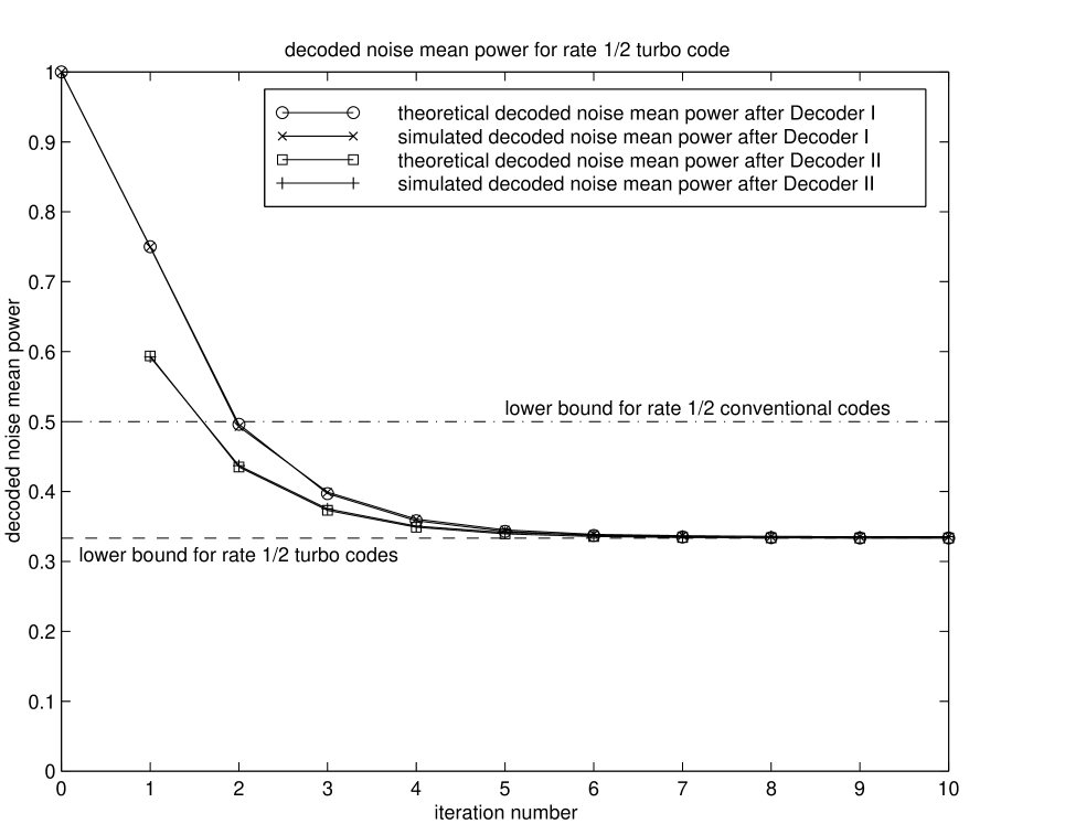
Figure 3: Decoded noise mean powers vs. iteration numbers for the rate 1/2 turbo code

for $i=1,2$. Certainly, they satisfy the condition in Corollary 2. The interleaver $P_{L}$ is the block interleaver with length $200\times 100=20000$ with row vectors (linewise) writing in and column vectors (columnwise) reading out, and $200$ by $100$ matrix size. The theoretical curves for both $\sigma_{1,l}^{2}$ (after Decoder I) and $\sigma_{2,l}^{2}$ (after Decoder II) in (3.22)-(3.23) of the decoded noise mean powers vs. iteration number $l$ are plotted in Fig. 3 with marks o and $\Box$, respectively. The corresponding simulated curves are also plotted in Fig. 3 with marks x and $+$, respectively. One can see that the simulated and theoretical curves coincide with each other. In Fig. 3, the lower bounds of the decoded noise mean powers for both turbo codes and the conventional codes with rate 1/2 are also shown. In this example, the lower bound in (3.34) on the number $l$ of the iterations in turbo codes is $1.4748$, i.e., when $l\geq 2$, the decoded noise mean power at the $l$th iteration is smaller than the ones for the conventional codes (the curves when $l\geq 2$ is below the lower bound $\sigma_{\eta}^{2}/2$ for rate $1/2$ non-turbo codes), which is precisely illustrated by the simulations shown in Fig. 3.

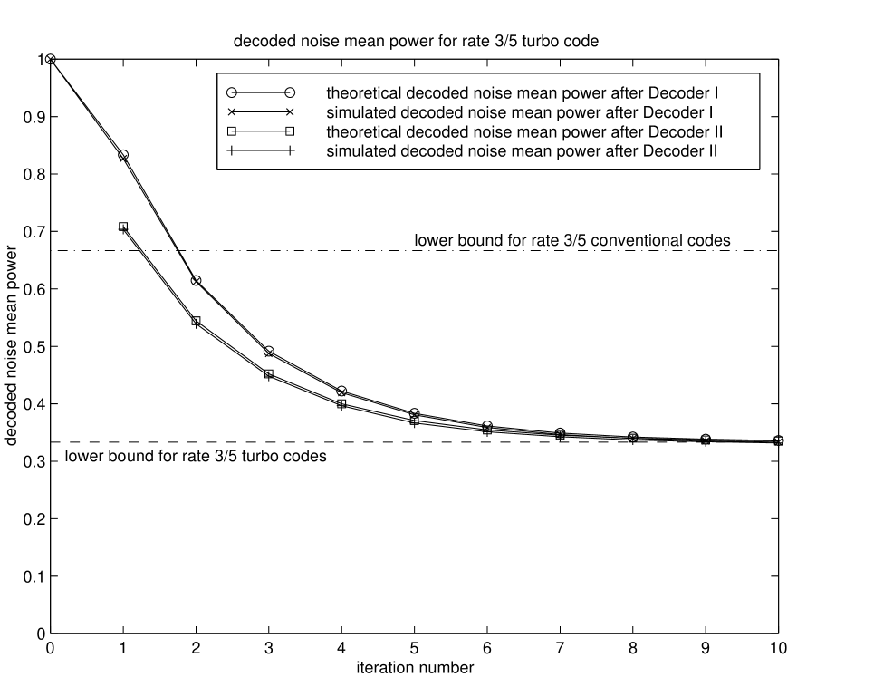
Figure 4: Decoded noise mean powers vs. iteration numbers for the rate 3/5 turbo code

The second turbo code is: $N_{1}=N_{2}=1$ and $K=3$, in this case, the turbo code rate is $3/5$. The two parallel codes are $G_{1}$ and $G_{2}$ with their parity check matrices $F_{1}=F_{2}=(1/\sqrt{3},1/\sqrt{3},-1/\sqrt{3})$ in (3.1), respectively. In this case, the three eigenvalues of $F_{i}^{\dagger}F_{i}$ are $1$, $0$ and $0$ for $i=1,2$. Similar to the first example, these codes also satisfy the condition in Corollary 2. The interleaver in this turbo code has length $600\times 50=30000$ and has the same type as the one in the first example. The theoretical and simulated curves of the decoded noise mean powers vs. the iteration number are plotted in Fig. 4. Similarly, the theoretical and simulated results coincide. Also, these curves converges to the same lower bound as the one in the first example, that is $\sigma_{\eta}^{2}/3$. This illustrates that the decoded noise mean power of turbo codes are eventually independent of the rates when the rates of the two parallel codes are less than $1/2$. However, one can clearly see from these two examples that the convergence speeds with different rates are different. In this example, the lower bound in (3.34) on the number $l$ of the iterations in turbo codes is $1.2047$, i.e., when $l\geq 2$, the decoded noise mean power at the $l$th iteration is smaller than the ones for the conventional codes, which is also precisely illustrated by the simulation shown in Fig. 4. Our numerous examples show that all the interleavers with square matrices do not perform well and actually the iterations may increase the decoded noise mean power, and the performance is sensitive to the choice of interleavers.

5 Conclusion

In this paper, we have analytically shown that the decoded noise mean power for turbo codes is smaller than the one for the conventional codes by extending them from finite fields to the complex field. It has been shown that the decoded noise mean power decreases when the iteration number increases in the iterative turbo code decoding, where the analytic decreasing rate has been given. We have also provided the limit of the decoded noise mean power in the iterative decoding. The limit is one third of the original noise power before the decoding, when the two parallel codes in turbo codes have rates less than $1/2$, which can not be achieved by any non-turbo codes with the same rate. All these results are built upon the assumption on the interleavers that decorrelates the decoded noises. From the results in this paper, the role of the interleavers is very clear. It turns out that the condition for the interleaver $P_{L}$ is that the operator $P_{L}^{-1}(I_{K}+F_{2}^{\dagger}F_{2})^{-1}P_{L}(I_{K}+F_{1}^{\dagger}F_{1})^{-1}$ maps a random process to another independent random process, where $(I_{K}+F_{i}^{\dagger}F_{i})^{-1}$ for $i=1,2$ are corresponding to the two cascaded decoders. The theoretical analysis has been illustrated by two numerical examples with rates 1/2 and 3/5. Our simulation results show that, after a few iteration decoding steps, the turbo code performance becomes better than the conventional code (non-turbo code) performance, and also the performance strongly depends on the choice of the interleavers.

Although the discussions in this paper are for codes defined on the complex field and from the digital signal processing point of view, it is believed that a similar analysis applies to codes defined on finite fields and even possibly a better performance can be achieved by taking the signal constellation and quantization into account. Further researches along this direction are under our current investigations.

This paper was written in the June of 1997.

References

[1] C. Berrou, A. Glavieux, and P. Thitimajshima, “Near Shannon limit error-correcting coding and decoding: turbo codes,” Proc. ICC’93, pp. 1064-1070, Geneve, Switzerland, May 1993.

[2] D. Divsalar and F. F. Pollara, “Turbo codes for PCS applications,” Proc. ICC’93, Seattle, WA, June 1995.

[3] P. Jung and M. Nasshan, “Performance evaluation of turbo codes for short frame transmission systems,” Electron. Lett., vol. 30, pp. 111-113, Jan. 1994.

[4] P. Jung and M. Nasshan, “Dependence of the error performance of turbo codes on the interleaver structure in short frame transmission systems,” Electron. Lett., vol. 30, pp. 287-288, Feb. 1994.

[5] S. Benedetto and G. Montorsi, “Average performance of parallel concatenated block codes,” Electron. Lett., vol. 31, pp. 156-158, Feb. 1995.

[6] S. Benedetto and G. Montorsi, “Performance evaluation of turbo-codes,” Electron. Lett., vol. 31, pp. 163-165, Feb. 1995.

[7] S. Benedetto and G. Montorsi, “Unveiling turbo codes: some results on parallel concatenated coding schemes,” IEEE Trans. on Information Theory, vol. 42, pp. 409-428, March 1996.

[8] J. Hagenauer, E. Offer, and L. Papke, “Iterative decoding of binary block and convolutional codes,” IEEE Trans. on Information Theory, vol. 42, pp. 429-445, March 1996.

[9] C. Berrou and A. Glavieux, “Near optimum error correcting coding and decoding: turbo codes,” IEEE Trans. on Communications, vol. 44, 1996.

[10] X.-G. Xia, “On modulated coding and least square decoding via coded modulation and Viterbi decoding,” technical report #97-6-2, Department of Electrical and Computer Engineering, University of Delaware, 1997.

[11] H. Liu and X.-G. Xia, “Precoding techniques for undersampled multi-receiver communication systems,” technical report #97-3-1, Department of Electrical Engineering, University of Delaware, 1997.

[12] X.-G. Xia and H. Liu, “Polynomial ambiguity resistant precoders: theory and applications in ISI/multipath cancellation,” technical report #97-5-1, Department of Electrical Engineering, University of Delaware, 1997.

[13] X.-G. Xia and G. Zhou, “On optimal ambiguity resistant precoders in ISI/multipath cancellation,” technical report #97-5-2, Department of Electrical Engineering, University of Delaware, 1997.

[14] Z. Xie, R. T. Short, and C. K. Rushforth, “A family of suboptimum detectors for coherent multiuser communications,” IEEE J. Select. Areas Communications, vol. 8, pp. 683-690, May 1990.

[15] U. Madhow and M. Honig, “MMSE interference suppression for direct-sequence spread spectrum CDMA,” IEEE Trans. on Communications, vol. 42, pp. 3178-3188, Dec. 1994.

[16] H. V. Poor and S. Verdú, “Probability of error in MMSE multiuser detection,” IEEE Trans. on Information Theory, vol. 43, pp. 858-871, May 1997.

[17] A. J. Viterbi, CDMA : Principles of Spread Spectrum Communication, Reading, Mass. : Addison-Wesley Pub. Co., 1995.

[18] IEEE Information Theory Society Newsletter, “A conversation with G. David Forney, Jr.,” vol. 47, No. 2, June 1997.