Nonparametric Additive Value Functions:
Interpretable Reinforcement Learning with an Application to Surgical Recovery

Abstract

We propose a nonparametric additive model for estimating interpretable value functions in reinforcement learning. Learning effective adaptive clinical interventions that rely on digital phenotyping features is a major for concern medical practitioners. With respect to spine surgery, different post-operative recovery recommendations concerning patient mobilization can lead to significant variation in patient recovery. While reinforcement learning has achieved widespread success in domains such as games, recent methods heavily rely on black-box methods, such neural networks. Unfortunately, these methods hinder the ability of examining the contribution each feature makes in producing the final suggested decision. While such interpretations are easily provided in classical algorithms such as Least Squares Policy Iteration, basic linearity assumptions prevent learning higher-order flexible interactions between features. In this paper, we present a novel method that offers a flexible technique for estimating action-value functions without making explicit parametric assumptions regarding their additive functional form. This nonparametric estimation strategy relies on incorporating local kernel regression and basis expansion to obtain a sparse, additive representation of the action-value function. Under this approach, we are able to locally approximate the action-value function and retrieve the nonlinear, independent contribution of select features as well as joint feature pairs. We validate the proposed approach with a simulation study, and, in an application to spine disease, uncover recovery recommendations that are inline with related clinical knowledge.

1 Introduction

The design and widespread usage of modern smartphones and wearables have facilitated real-time and consistent access to data concerning human behavior and health [46, 32]. Digital phenotyping data offers a resource for clinicians interested in learning improved guidelines and recommendations for patients recovering from clinical or surgical procedures [9, 35]. Currently, questions concerning a patient’s quality of life after a treatment or surgery are largely inferred from in-person follow-up visits and infrequent electronic surveys. These methods of evaluation are severely limited due their reliance on patient recall and their inability to capture the temporal evolution of a patient’s recovery. By combining the utility of digital phenotyping and novel statistical machine learning techniques, clinical practitioners are afforded a new paradigm for discovering improved standards of care from high-quality and temporally-dense data [36].

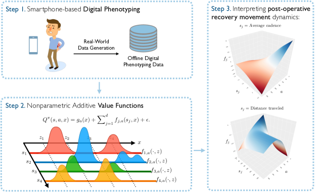
Figure 1: An overview of using nonparametric additive models for learning interpretable value functions. Within our setting, real-world data from subjects with select physiological disorders are collected using a smartphone-based digital phenotyping platform. Modalities collected from subject smartphones range from raw sensor data (e.g., GPS, accelerometer, gyroscope, or magnetometer) to usage logs (e.g., anonymized communication and screen-time). Relevant features $\mathbf{s}=(s_{1},\dots,s_{d})^{T}$ are summarized from these modalities and are used to frame a corresponding decision-making problem (or MDP see 2.1) of interest. Under the select MDP, we model the value function $Q^{\pi}(\mathbf{s},a,x)$ as a sum of nonparametric component functions $g_{a}(x)$ and $f_{j,a}(\mathbf{s}_{j},x)\hskip 3.0pt\forall j$. Here we visualize the change in the shape and sparsity patterns of the component function $f_{j,a}(\cdot,z)$ as the candidate variable $x$ changes, e.g., $x\in\{z_{1},z_{2},z_{3},z_{4}\}$. Each additive component function can be estimated and inspected using the kernel-weighted least square fixed point approximation detailed in 3.

In this paper, we introduce a novel approach in reinforcement learning for estimating recovery strategies and recommendations in studies employing the use of digital phenotyping data. Reinforcement learning is a sub-field of machine learning that focuses on learning sequences of decisions that optimize long-term outcomes from experiential data [45]. Within healthcare, reinforcement learning algorithms have been used to discover decision-making strategies for chronic illness treatments [5, 38], anesthesia regulation and automation [43], chemotherapy scheduling and dosage management [34, 1], and sepsis management [39, 37].

As it stands, employing reinforcement learning algorithms for healthcare applications requires (1) a consideration of the process used to estimate the decision-making strategy, or policy $\pi$, and (2) the ability to carefully examine the intended behavior of the learned policy before deployment in the real world [16]. Within these settings, decision-making policies are commonly represented as a function $\pi(\mathbf{s})$ of state features $\mathbf{s}=(s_{1},\dots,s_{d})^{T}\in\mathbb{R}^{d}$. Accordingly, policies can be estimated using policy gradient or value-based reinforcement learning algorithms [45]. In value-based reinforcement learning, policies are determined by selecting the action $a$ that maximizes the corresponding action-value function $Q^{\pi}(\mathbf{s},a)$. Under this greedy action-selection strategy, retrieving an optimal policy relies on learning an optimal action-value function, commonly represented using neural network function approximators. As such, current value-based reinforcement learning algorithms serve as black boxes that simply receive a set of data and output a near-optimal policy. Generally, these polices are not only difficult to interpret, but provide minimal indication as to which features in the data (i.e., $\mathbf{s}_{j}\hskip 3.0pt\forall j\in[d]$) contributed to the selected decision [16].

Rather than relying on black box function approximators, we introduce a class of value functions that provides a flexible, nonparametric representation of the action-value function, easily interpretable for both researchers and clinicians. By allowing for the inspection of a candidate variable $x$ (i.e., time-varying/-invariant confounders or continuous-valued actions), we construct a generalized framework for modeling action-value functions as a sum of nonparametric, additive component functions and takes the form

$$Q^{\pi}(\mathbf{s},a,x) =g_{a}(x)+\sum_{j=1}^{d}f_{j,a}(\mathbf{s}_{j},x)+\epsilon.$$ (1.1)

Specifically, we extend in the input space of $Q^{\pi}$ and allow for the examination of the marginal effect of a candidate variable $x$, as well as its joint effect between state features $\mathbf{s}_{j}$ under a discretized action space. This framework allows us to explore several representations of each additive component depending on our choice of $x$. For instance, when $x$ takes on continuous values over the entire discretized action space of $a$, we can directly represent $x$ as the continuous action $a$ and equate the marginal and joint additive component functions in Equation 1.1 to $g(a)$ and $f_{j}(\mathbf{s}_{j},a)$, respectively.

To estimate the components functions, we consider the classical approximate policy iteration algorithm, Least Square Policy Iteration (LSPI) [26], and provide a kernel-hybrid approach for estimating action-value functions without making explicit parametric assumptions regarding their additive functional form. To do so, we relax the traditional linearity assumption imposed in LSPI by leveraging advances in estimating high dimensional, nonparametric additive regression models [12, 40, 25]. In particular, we propose incorporating the kernel-sieve hybrid regression estimator introduced in [28] to obtain a sparse additive representation of the action-value function by combining local kernel regression and basis expansion methods such as splines.

To demonstrate the applicability of our methodology, we provide a simulation study, where we examine its ability in estimating nonlinear additive functions and compare its performance against modern neural network-based approaches. Furthermore, we directly apply our model to an on-going digital phenotyping study, where we learn and interpret a decision-making policy that aims to improve pain management and functional recovery in patients recovering from spine surgery by managing on patient mobility.

1.1 Related Research

Our work directly contributes to the growing literature on function approximation methods for value-based reinforcement learning. Current state-of-the-art algorithms approximate action-values functions using expressive modeling architectures such as neural networks. By combining fitted Q-iteration procedure with modern tools such as replay buffers and target networks, these algorithms are able to resolve the pitfalls of classical methods and solve complex, high-dimensional decision-making tasks [42, 2, 48, 29, 30]. Unfortunately, the powerful flexibility of these approaches comes at the cost of interpretability that is native to algorithms such as Least Squares Policy Iteration (LSPI).

LSPI is a model free, off-policy approximate policy iteration algorithm that models the action-value function using a parametric linear approximation and finds an approximate function that best satisfies the Bellman equation (i.e., the fixed point solution) [26]. While LSPI provides an unbiased estimate of the action-value function, it faces significant challenges when the model is misspecified and when the dimensionality of the feature space is high [26, 13]. Several modifications to LSPI have been proposed in the reinforcement learning literature. In settings where the feature space is large, several approach exist for finding sparse solutions under a linear model [18, 23, 47, 14]. Alternatively, [51] propose a kernel-based LSPI algorithm that operates in an infinite dimensional Hilbert space and allows for nonlinear feature extraction by selecting appropriate kernel functions. Additionally, [19] propose a locally-weighted LSPI model that leverages locally-weighted to construct a nonlinear, global control policy. In general, these last two approaches avoid the pitfalls of model misspecification and minimize apriori knowledge needed to model the action-value function.

Currently, no approximation methods in RL has been introduced that direcly allows for the nonparametric estimation concerning the additive contribution of select features and joint feature pairs. In the supervised learning literature, several approaches exist for estimating nonparametric component functions under high-dimensional feature spaces. Several of these approaches include generalized additive models (GAM) and sparse additive models (SpAM), which our approach draws parallels to [40, 17]. To bridge these areas of research, we re-formulate the policy evaluation step of the classical LSPI algorithm and propose incorporating the kernel-sieve hybrid regression estimator introduced in [28]. This approach provides a powerful function approximation technique for locally estimating action-value functions using a loss function combining both basis expansion and kernel method with a hybrid $\ell_{1}/\ell_{2}$-group Lasso penalty.

1.2 Organization of the Paper

The remainder of this paper is organized as follows. In Section 2.2, we introduce our generalized, nonparametric model for representing action-value functions. In Section 3, we present our estimation strategy for locally approximating the action-value function by combining basis expansion and kernel methods. In Section 4, we examine the results of a simulation study and highlight our method’s performance in estimating the sparse additive components of the action-value function. In Section 5, we present a real-world cohort of patients recovering from a neurological intervention for spine disease as a motivating case study. In Section 6, we apply our method to the digital-phenotyping study described in Section 5 and interpret the estimated recovery strategy. In Section 7, we discuss the limitations of our method and propose future extensions to address them.

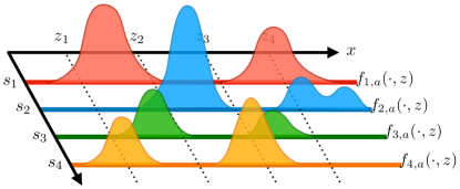
Figure 2: Representation of a nonparametric additive value function $Q^{\pi}(\mathbf{s},a,x)$ with respect to the candidate variable $x$ as detailed in (2.4).

2 Nonparametric Additive Value Functions

2.1 Preliminaries and Notation

We consider a discrete time, infinite horizon Markov Decision Process (MDP) defined by the tuple $\{\mathcal{S},\mathcal{A},\mathcal{P},R,\gamma\}$, where $\mathcal{S}$ is a $d$-dimensional continuous state space, $\mathcal{A}$ is a set of discrete (i.e., $\mathcal{A}=\{1,\dots,k\}$) or continuous (i.e., $\mathcal{A}=\mathbb{R}$) actions, $\mathcal{P}(\mathbf{s}^{\prime}|\mathbf{s},a)$ is a next-state transition probability kernel that specifies the probability of transitioning from state $\mathbf{s}\in\mathcal{S}$ to the next state $\mathbf{s}^{\prime}\in\mathcal{S}$ after taking action $a\in\mathcal{A}$, $R:\mathcal{S}\times\mathcal{A}\rightarrow\mathbb{R}$ is a reward function, and $\gamma\in[0,1]$ is a discount factor for weighting long-term rewards. Within this stochastic environment, the action selection strategy is determined by a deterministic policy, $\pi:\mathcal{S}\rightarrow\mathcal{A}$.

To assess the quality of a policy, the expected discounted sum of rewards when starting at state $\mathbf{s}$ and following policy $\pi$ can be computed using the value function $V^{\pi}:\mathcal{S}\rightarrow\mathbb{R}$. The value function starting a state $\mathbf{s}$ is defined as

$$V^{\pi}(\mathbf{s})=\mathbb{E}_{\pi}\left[\sum_{i=0}^{\infty}\gamma^{i}r_{i}\mid\mathbf{s}_{\text{init}}=\mathbf{s}\right].$$ (2.1)

In control problems where we are interested in improving our action selection strategy, it is useful to consider the action-value function $Q^{\pi}:\mathcal{S}\times\mathcal{A}\rightarrow\mathbb{R}$. Given a policy $\pi$, $Q^{\pi}$ represents the expected discounted sum of rewards after taking action $a$ and state $\mathbf{s}$, and following policy $\pi$ thereafter, i.e.,

$$Q^{\pi}(\mathbf{s},a)=\mathbb{E}_{\pi}\left[\sum_{i=0}^{\infty}\gamma^{i}r_{i}\mid\mathbf{s}_{\text{init}}=\mathbf{s},a_{\text{init}}=a\right]$$ (2.2)

Due to the Markovian property of our MDP, the action-value function (as well as the value function) is a fixed point of the Bellman operator $Q^{\pi}=\mathcal{T}_{\pi}Q^{\pi}$, where the operator $\mathcal{T}_{\pi}$ is defined as

$$(\mathcal{T}_{\pi}Q)(\mathbf{s},a)=R(\mathbf{s},a)+\gamma\int_{\mathcal{S}}Q(\mathbf{s}^{\prime},\pi(\mathbf{s}^{\prime}))d\mathcal{P}(\mathbf{s}^{\prime}|\mathbf{s},a)$$ (2.3)

or, equivalently in vector form, as $\mathcal{T}_{\pi}Q=\mathcal{R}+\gamma\mathcal{P}^{\pi}Q$, where $\mathcal{R}\in\mathbb{R}^{|\mathcal{S}||\mathcal{A}|}$ is a reward vector and $\mathcal{P}^{\pi}\in\mathbb{R}^{|\mathcal{S}||\mathcal{A}|\times|\mathcal{S}||\mathcal{A}|}$ is the induced transition matrix when following policy $\pi$ after a next state transition according to $\mathcal{P}(\mathbf{s}^{\prime}|\mathbf{s},a)$.

For a given MDP, the optimal action-value function is defined as $Q^{*}(\mathbf{s},a)=\sup_{\pi}Q^{\pi}(\mathbf{s},a)$ for all states and actions $(\mathbf{s},a)\in\mathcal{S}\times\mathcal{A}$. For a given action-value function $Q$, we define a greedy policy $\pi$ as $\pi(\mathbf{s})=\arg\max_{a\in\mathcal{A}}Q(\mathbf{s},a)$ for all $\mathbf{s}\in\mathcal{S}$. The greedy policy with respect to the optimal action-value function $Q^{*}$ is then an optimal policy, denoted as $\pi^{*}$. Hence, obtaining $Q^{*}$ allows us to arrive at an optimal action selection strategy.

2.2 Generalized Framework

For an arbitrary policy $\pi$, we introduce a generalized framework for modeling the action-value function $Q^{\pi}$ as a sum of nonparametric additive component functions. Our approach handles both discrete (i.e., $\mathcal{A}=\{1,\dots,k\}$) and continuous (i.e., $\mathcal{A}\equiv\mathbb{R}$) action spaces, while allowing for the incorporation of potentially time-varying, or time-invariant variables.

First, we present our generalized nonparametric framework for modeling $Q^{\pi}$ as

$$Q^{\pi}(\mathbf{s},a,x) =g_{a}(x)+\sum_{j=1}^{d}f_{j,a}(\mathbf{s}_{j},x)+\epsilon.$$ (2.4)

Under this model, we expand the input space of $Q^{\pi}$ to include the candidate variable $x\in\mathbb{R}$, and discretize the action space such that $a\in\{1,\dots,k\}$ if $\mathcal{A}$ is not already discrete. Accordingly, $g_{a}(\cdot)$ represents the additive marginal effect of $x$ under action $a$, and $f_{j}(\cdot,\cdot)$ represents the additive joint effect of interactions between $x$ and state features $\mathbf{s}_{j}$ under action $a$. Without making assumptions on the functional form of $g_{a}(\cdot)$ and $f_{j,a}(\cdot,\cdot)$, our model allows us to carefully examine additive nonlinear relationships that exist among relevant state features, actions and the variable $x$.

Second, our choice in $x$ allows us to explore several unique representations of the additive components in (2.4). For example, $x$ can represent time-varying or time-invariant confounders (e.g., age, gender, or the number of days since a surgical event) as well as continuous-valued actions $a\in\mathbb{R}$:

$$x=\begin{cases}\hskip 2.0pt\mathbf{s}_{0},\hskip 4.0pt\text{i.e., a candidate state feature or confounder,}\\ \hskip 2.0pta,\hskip 8.0pt\text{i.e., a continuous action}\end{cases}.$$ (2.5)

Example 2.1.

When $x=\mathbf{s}_{0}$, the additive functions in (2.4) respectively equate to $g_{a}(x)=g_{a}(\mathbf{s}_{0})$ and $f_{j,a}(\mathbf{s}_{j},x)=f_{j,a}(\mathbf{s}_{j},\mathbf{s}_{0})$. Furthermore, we can augment the state space $S$ using $x$ to form $S_{+}=\{x,s_{1},\dots,s_{d}\}$, and succinctly represent $Q^{\pi}(\mathbf{s},a,\mathbf{s}_{0})$ as $Q^{\pi}(\mathbf{s}_{+},a)$, where $\mathbf{s}_{+}\in S_{+}$ and

$$Q^{\pi}(\mathbf{s}_{+},a) =g_{a}(\mathbf{s}_{0})+\sum_{j=1}^{d}f_{j,a}(\mathbf{s}_{j},\mathbf{s}_{0})+\epsilon.$$ (2.6)

Thus, under the discrete action $a$, $g_{a}(\mathbf{s}_{0})$ models the nonlinear marginal effect of the confounder or state feature $\mathbf{s}_{0}$, whereas $f_{j,a}(\mathbf{s}_{j},\mathbf{s}_{0})$ models the nonlinear interaction between $\mathbf{s}_{0}$ and state features $\mathbf{s}_{j}$.

Example 2.2.

Similarly, when $x=a$, the additive functions in (2.4) respectively equate to $g_{a}(a)=g(a)$ and $f_{j,a}(\mathbf{s}_{j},a)=f_{j}(\mathbf{s}_{j},a)$. Under this choice of $x$, we avoid explicit discretization of the action space $\mathcal{A}$ and directly treat $a$ as a continuous action. Thus, for a given state-action pair, $Q^{\pi}(\mathbf{s},a,a)$ reduces to $Q^{\pi}(\mathbf{s},a)$, where

$$Q^{\pi}(\mathbf{s},a) =g(a)+\sum_{j=1}^{d}f_{j}(\mathbf{s}_{j},a)+\epsilon,$$ (2.7)

and the additive marginal effect of selecting a continuous action $a$ is modeled as $g(a)$, and $f_{j}(\mathbf{s}_{j},a)$ represents the additive effect of selecting action $a$ under state feature value $\mathbf{s}_{j}$.

3 Kernel Sieve Hybrid - Least Squares Policy Iteration

We introduce a general approach for estimating $Q^{\pi}(\mathbf{s},a)$ for both discrete and continuous action spaces. This estimation strategy offers us an intuitive way to (1) locally approximate the action-value function as an additive model with independent state features spanned by a B-spline basis expansion, (2) retrieve an estimate of the nonlinear additive components, and (3) obtain a sparse representation of the action-value function by selecting relevant regions of the domain of the component functions.

3.1 Basis Expansion

First, we model the action-value function using a centered B-spline basis expansion of the additive component functions. Let $\{\psi_{1},\dots,\psi_{m}\}$ be a set of normalized B-spline basis functions. For each component function, we project $f_{j,a}$ onto the space spanned by the basis, $\mathcal{B}_{m}=\text{Span}(\psi_{1},\dots,\psi_{m})$. Accordingly, $f_{j,a}(\mathbf{s}_{j},x)=\sum_{\ell=1}^{m}\varphi_{j\ell}(\mathbf{s}_{j})\bm{\beta}_{j\ell;a}(x)$, where $\varphi_{j\ell}$ are locally centered B-spline basis functions defined as $\varphi_{j\ell}(\mathbf{s})=\psi_{\ell}(\mathbf{s})-E[\psi_{\ell}(\mathbf{s}_{j})]$ for the $j$-th component function and the $\ell$-th basis component.

As we will discuss in Section 3.2, our estimation strategy relies on performing a locally-weighted least-squares minimization of an objective criterion with respect to a fixed value of the variable $x$. As such, we locally express our model in $(\ref{general-model})$ by (i) setting $x=z$, where $z\in\mathcal{X}$ is some arbitrary fixed value, and by (ii) using the aforementioned centered B-spline basis expansion:

$$Q^{\pi}(\mathbf{s},a,x=z)\approx\alpha_{a,z}+\sum_{j=1}^{d}\sum_{\ell=1}^{m}\varphi_{j\ell}(\mathbf{s}_{j})\beta_{j\ell;a,z}\quad.$$ (3.1)

Under this local model, $\alpha_{a,z}\in\mathbb{R}$ represents that marginal effect $g_{a}(x)$ when $z$ is a fixed value of $x$. Accordingly, $\beta_{j\ell;a,z}\in\mathbb{R}$ is the coordinate corresponding to the $\ell$-th B-spline basis of the $j$-th state-feature under $z$.

In Examples 2.1 and 2.2, we observe two choices for representing $x$ that highlight the generalizability of our model structure. Under theses examples, the local additive components in (3.1) can also be re-expressed as follows:

$$\alpha_{a,z}=\begin{cases}\hskip 2.0pt\alpha_{a,z}\hskip 8.0pt\text{when}\hskip 4.0ptx=\mathbf{s}_{0},\hskip 4.0pt\\ \hskip 2.0pt\alpha_{z}\hskip 15.0pt\text{when}\hskip 4.0ptx=a\end{cases}\quad\text{and}\quad\beta_{j\ell;a,z}=\begin{cases}\hskip 2.0pt\beta_{j\ell;a,z}\hskip 8.0pt\text{when}\hskip 4.0ptx=\mathbf{s}_{0},\hskip 4.0pt\\ \hskip 2.0pt\beta_{j\ell;z}\hskip 15.0pt\text{when}\hskip 4.0ptx=a\end{cases}.$$ (3.2)

Since the dynamics of the MDP are unknown, our estimation strategy relies on a batch dataset $\mathcal{D}=\{(\mathbf{s}^{[i]},a^{[i]},r^{[i]},\mathbf{s}^{[i]}{{}^{\prime}},x^{[i]})\}_{i=1}^{N}$ of sampled transitions from the MDP of interest, where $\mathbf{s}^{[i]}{{}^{\prime}}\sim P(\cdot|\mathbf{s}^{[i]},a^{[i]})$, and $x^{[i]}$ is the associated value of the candidate variable $x$. When we consider all observations in the dataset $\mathcal{D}$, we can equivalently re-express (3.1) in vector form as

$$Q_{\bm{\beta}_{+}}^{\pi}=\widetilde{\bm{\Phi}}\bm{\beta}_{+}$$ (3.3)

where $\bm{\beta_{+}}=(\bm{\beta}_{1+}^{T},\dots,\bm{\beta}_{|\mathcal{A}|+}^{T})^{T}$ $\in\mathbb{R}^{(1+dm)|\mathcal{A}|}$, $\bm{\beta}_{a+}=(\alpha_{a,z},\bm{\beta}_{1;a,z}^{T},\dots,\bm{\beta}_{d;a,z}^{T})^{T}\in\mathbb{R}^{1+dm}$, and

$$\widetilde{\bm{\Phi}}=\left(\begin{array}[]{c}\phi\left(\mathbf{s}^{[1]},a^{[1]},\right)^{T}\\ \vdots\\ \phi\left(\mathbf{s}^{[N]},a^{[N]},\right)^{T}\end{array}\right)=\left(\begin{array}[]{c}\varphi_{+}\left(\mathbf{s}^{[1]}\right)^{T}\mathbb{1}(a^{[1]}=1)\cdots\varphi_{+}\left(\mathbf{s}^{[1]}\right)^{T}\mathbb{1}(a^{[1]}=k)\\ \vdots\\ \varphi_{+}\left(\mathbf{s}^{[N]}\right)^{T}\mathbb{1}(a^{[N]}=1)\cdots\varphi_{+}\left(\mathbf{s}^{[N]}\right)^{T}\mathbb{1}(a^{[N]}=k)\end{array}\right)$$ (3.10)

such that $\widetilde{\bm{\Phi}}\in\mathbb{R}^{N\times(1+dm)|\mathcal{A}|}$, $\varphi_{+}(\mathbf{s})=\big{(}1\hskip 5.0pt\varphi_{2}(\mathbf{s}_{1})\cdots\varphi_{d}(\mathbf{s}_{d})\big{)}^{T}\in\mathbb{R}^{1+dm}$ and $\varphi_{j}(\mathbf{s}_{j})\in\mathbb{R}^{m}$ is a B-spline basis component vector. Note that $E[\psi_{\ell}(\mathbf{s}_{j})]$ is estimated as $\bar{\psi}_{j\ell}=N^{-1}\sum_{i=1}^{N}\psi_{\ell}(\mathbf{s}_{j}^{[i]})$ by using a sample of $N$ data points from the dataset $\mathcal{D}$.

3.2 Kernel-Weighted Least Squares Fixed Point Approximation

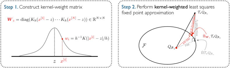
Figure 3: A step-by-step illustration of kernel-weighted least squares fixed point approximation. First, using observations gathered in the batch dataset $\mathcal{D}$, we construct a diagonal kernel-weight matrix $\bm{W}_{z}$, where each diagonal weight is a function of the distance between the observed candidate variable $x^{[i]}$ and the fixed value $z$. Second, let $\mathcal{F}$ be $\mathcal{C}(\bm{\Phi})$, i.e., the space of approximate value functions. Since applying the Bellman operator $\mathcal{T}_{\pi}$ to an arbitrary value function $Q_{\bm{\beta}_{+}}$ can push the resulting quantity $\mathcal{T}_{\pi}Q^{\pi}_{\bm{\beta}_{+}}$ out of the space $\mathcal{F}$, we perform a projection step using the constructed kernel-weighted matrix $\bm{W}_{z}$ (detailed in 3.2). This approach differs from classical least squares fixed point approximation (shown in grey), where an $\ell_{2}$-projection operator $\widehat{\Pi}$ is used. Lastly, we find $\widehat{\bm{\beta}}_{+}$ that minimizes the $\ell_{2}$-norm between $Q_{\bm{\beta}_{+}}$ and $\widehat{\Pi}_{\bm{W}_{z}}\mathcal{T}_{\pi}Q^{\pi}_{\bm{\beta}_{+}}$, i.e., the kernel-weighted projected bellman error.

We estimate our model parameters $\bm{\beta}_{+}$ by minimizing a kernel-weighted version of the classical projected Bellman error (PBE).

In LPSI, we observe that a simple procedure for estimating a linear action-value function is to force the approximate function to be a fixed point under the projected Bellman operator (i.e., $\Pi\mathcal{T}_{\pi}Q_{\bm{\beta}_{+}}\approx Q_{\bm{\beta}_{+}}$). For this condition to hold, the fixed point of the Bellman operator $\mathcal{T}_{\pi}$ must lie in the space of approximate value functions spanned by the basis functions over all possible state-action pairs, $\mathcal{C}(\bm{\Phi})$. By construction, it is known that $Q_{\bm{\beta}_{+}}=\bm{\Phi}\bm{\beta}_{+}\in\mathcal{C}(\bm{\Phi})$. However, since there is no guarantee that $\mathcal{T}_{\pi}Q_{\bm{\beta}_{+}}$ (i.e., the result of the Bellman operator) is in $\mathcal{C}(\bm{\Phi})$, it first must be projected onto $\mathcal{C}(\bm{\Phi})$ using the projection operator $\Pi$, such that $\Pi\mathcal{T}_{\pi}Q^{\pi}_{\bm{\beta}_{+}}=\bm{\Phi}\bm{u}^{*}$ where $\bm{u}^{*}$ is the solution to the following least-squares problem

$$\bm{u}^{*} =\mathop{\mathrm{argmin}}_{Q\in\mathcal{C}(\bm{\Phi})}\|Q_{\bm{\beta}_{+}}-\mathcal{T}_{\pi}Q_{\bm{\beta}_{+}}\|_{2}^{2}=\mathop{\mathrm{argmin}}_{\bm{u}\in\mathbb{R}^{k}}\|\bm{\Phi}u-\mathcal{T}_{\pi}\bm{\Phi}\bm{\beta}_{+}\|_{2}^{2}.$$ (3.11)

Empirically, $\bm{u}^{*}$ can be estimated using a sample-based feature design matrix $\widetilde{\bm{\Phi}}$ constructed from a dataset of $N$ transitions $\mathcal{D}$,

$$\bm{u}^{*} =\mathop{\mathrm{argmin}}_{\bm{u}\in\mathbb{R}^{k}}\|\widetilde{\bm{\Phi}}\bm{u}-\widehat{\mathcal{T}}_{\pi}\widetilde{\bm{\Phi}}\bm{\beta}_{+}\|_{2}^{2}$$ (3.12)

$$=\mathop{\mathrm{argmin}}_{\bm{u}\in\mathbb{R}^{k}}\sum_{i=1}^{N}\left(\phi(\mathbf{s}^{[i]},a^{[i]})^{T}\bm{u}-\Big{[}r^{[i]}+\gamma\phi(\mathbf{s}^{[i]}{{}^{\prime}},\pi(\mathbf{s}^{[i]}{{}^{\prime}}))^{T}\bm{\beta}_{+}\Big{]}\right)^{2}$$ (3.13)

where $\widehat{\mathcal{T}}_{\pi}$ is the empirical Bellman operator $(\widehat{\mathcal{T}}_{\pi}Q_{\beta})(\mathbf{s},a)=r(\mathbf{s},a)+\gamma\hskip 2.0ptQ_{\beta}(\mathbf{s}^{\prime},\pi(\mathbf{s}))$ defined using a single transition $\{\mathbf{s},a,r,\mathbf{s}^{\prime}\}$ from $\mathcal{D}$.

Rather than performing the projection step according to an $\ell_{2}$-norm, we propose using a kernel-weighted norm with weights that are centered at a fixed value $z$ that lies within the domain of the candidate variable $x$. Let the $K:\mathcal{X}\rightarrow\mathbb{R}$ be a symmetric kernel function with bounded support. We denote $K_{h}(\cdot)=h^{-1}K(\cdot/h)$, where $h>0$ is the bandwidth. The solution $\bm{u}_{z}^{*}$ to the kernel-weighted projection step is estimated as follows

$$\bm{u}_{z}^{*} =\mathop{\mathrm{argmin}}_{\bm{u}\in\mathbb{R}^{k}}\sum_{i=1}^{N}K_{h}(x^{[i]}-z)\left(\phi(\mathbf{s}^{[i]},a^{[i]})^{T}\bm{u}-\Big{[}r^{[i]}+\gamma\phi(\mathbf{s}^{[i]}{{}^{\prime}},\pi(\mathbf{s}^{[i]}{{}^{\prime}}))^{T}\bm{\beta}_{+}\Big{]}\right)^{2}$$ (3.14)

$$=\mathop{\mathrm{argmin}}_{\bm{u}\in\mathbb{R}^{k}}\left(\widetilde{\bm{\Phi}}\bm{u}-\widehat{\mathcal{T}}_{\pi}\widetilde{\bm{\Phi}}\bm{\beta}_{+}\right)^{T}\bm{W}_{z}\left(\widetilde{\bm{\Phi}}\bm{u}-\widehat{\mathcal{T}}_{\pi}\widetilde{\bm{\Phi}}\bm{\beta}_{+}\right)=(\widetilde{\bm{\Phi}}^{T}\bm{W}_{z}\widetilde{\bm{\Phi}})^{-1}\widetilde{\bm{\Phi}}^{T}\bm{W}_{z}\widehat{\mathcal{T}}_{\pi}\widetilde{\bm{\Phi}}\bm{\beta}_{+},$$ (3.15)

where $\bm{W}_{z}=\operatorname{diag}(K_{h}(x^{[1]}-z)\cdots K_{h}(x^{[N]}-z))\in\mathbb{R}^{N\times N}$ is a diagonal kernel-weight matrix. Under this weighted norm, transitions with a candidate variable $x^{[i]}$ that are local to $z$ contribute more to the overall fit of the least squares minimization. Accordingly, the empirical kernel-weighted projection operator is $\widehat{\Pi}_{\bm{W}_{z}}=\widetilde{\bm{\Phi}}(\widetilde{\bm{\Phi}}^{T}\bm{W}_{z}\widetilde{\bm{\Phi}})^{-1}\widetilde{\bm{\Phi}}^{T}\bm{W}_{z}$.

Using the projection operator $\widehat{\Pi}_{\bm{W}_{z}}$, we can now directly find $\bm{\beta_{+}}$ that minimizes the kernel-weighted empirical PBE represented as

$$\mathcal{E}_{\mathcal{D}}=\|Q_{\bm{\beta}_{+}}^{\pi}-\widehat{\Pi}_{\bm{W}_{z}}\mathcal{T}_{\pi}Q^{\pi}_{\bm{\beta}_{+}}\|_{2}^{2}=\|\widetilde{\bm{\Phi}}\bm{\beta}_{+}-\widetilde{\bm{\Phi}}\underbrace{(\widetilde{\bm{\Phi}}^{T}\bm{W}_{z}\widetilde{\bm{\Phi}})^{-1}\widetilde{\bm{\Phi}}^{T}\bm{W}_{z}\mathcal{T}_{\pi}\widetilde{\bm{\Phi}}\bm{\beta}_{+}}_{\widetilde{g}(\bm{\beta}_{+})\in\mathbb{R}^{k}}\|_{2}^{2}.$$ (3.16)

Since $\widetilde{\bm{\Phi}}\widetilde{g}(\beta)\in\mathcal{C}(\widetilde{\bm{\Phi}})$, minimizing this objective function is equivalent to solving for $\bm{\beta}_{+}$ in $\bm{\Phi}\bm{\beta}_{+}=\bm{\Phi}\widetilde{g}(\bm{\beta}_{+})$, which can be simplified as

$$\underbrace{\widetilde{\bm{\Phi}}^{T}\bm{W}_{z}\big{(}\widetilde{\bm{\Phi}}-\gamma\widetilde{\bm{\Phi}}^{\prime}\big{)}}_{\bm{A}_{z}}\bm{\beta}_{+}=\underbrace{\widetilde{\bm{\Phi}}^{T}\bm{W}_{z}\widetilde{R}}_{\bm{b}_{z}},$$ (3.17)

where $\widetilde{\bm{\Phi}}^{\prime}=\left(\phi(\mathbf{s}^{[1]}{{}^{\prime}},\pi(\mathbf{s}^{[1]}{{}^{\prime}}))^{T}\hskip 2.0pt\cdots\hskip 4.0pt\phi(\mathbf{s}^{[N]}{{}^{\prime}},\pi(\mathbf{s}^{[N]}{{}^{\prime}}))^{T}\right)^{T}$. Thus, the solution to minimizing the kernel-weighted empirical PBE can be obtained analytically as $\widehat{\bm{\beta}}_{+}=\bm{A}_{z}^{-1}\bm{b}_{z}$. This procedure is summarized in Figure 3.

3.3 Component-wise Regularization via Group Lasso

Since we are interested in obtaining a sparse representation of the elements in $\bm{\beta}_{+}$, we apply a penalty to an estimating equation $\mathcal{L}_{z}(\bm{\beta}_{+})$ of (3.17). Being that components of our basis functions are grouped by features, we incorporate a group Lasso penalty that performs group level variable selection by jointly constraining all coefficients that belong to a given feature. Consequently, our primary objective function for our estimator is

$$\mathcal{L}_{z}(\bm{\beta}_{+})+\lambda\mathcal{R}(\bm{\beta}_{+})=-\frac{1}{2}\bm{\beta}_{+}^{T}\widetilde{\bm{A}}_{z}\bm{\beta}_{+}-\bm{\beta}_{+}^{T}\widetilde{\bm{b}}_{z}+\lambda\sum_{a}^{|\mathcal{A}|}\Big{(}\sqrt{m}\cdot|\alpha_{a}|+\sum_{j\geq 2}\left\|\bm{\beta}_{j;a}\right\|_{2}\Big{)},$$ (3.18)

where $\lambda$ is a regularization parameter. Note that the group Lasso penalty $\mathcal{R}(\bm{\beta}_{+})$ includes a $\sqrt{m}$ factor used to appropriately scale the strength of the regularization term $\lambda$ applied to $|\alpha_{a}|$ and to that of the coefficients of the B-splines basis functions. This ensures that the grouped coefficients gets evenly penalized.

Input: $z$ (Fixed value), $\bm{\beta}^{(0)}_{+}$ (Initial weights), $K(\cdot)$ (Kernel function), $0\leq\gamma<1$ (Discount factor), $\mu$ (Step size), $\epsilon$ (Stopping Criteria), $\lambda$ (Regularization Parameter), $\pi$ (Current Policy)

[0.45em] Data: Dataset of transitions $\mathcal{D}=\{(\mathbf{s}^{[i]},a^{[i]},r^{[i]},\mathbf{s}^{[i]}{{}^{\prime}},x^{[i]})\}_{i=1}^{N}$

[0.45em] Initialization: Construct $\bm{W}_{z}$, $\bm{\Phi}$ and $\bm{\Phi}^{\prime}$

while $||\bm{\beta}^{(t+1)}_{+}-\bm{\beta}^{(t)}_{+}||\geq\epsilon$ do

       Select $j\in[d]$ with probability $1/d$

       for $a\in\mathcal{A}$ do

             Update $\bm{\beta}^{(t+1)}_{j,a}\leftarrow\mathcal{U}_{\lambda_{j}/\mu}\left(\bm{\beta}_{j;a}^{(t)}-\mu\hskip 2.0pt\bm{\Phi}^{T}_{\mathchoice{\mathbin{\vbox{\hbox{\scalebox{0.5}{$\displaystyle\bullet$}}}}}{\mathbin{\vbox{\hbox{\scalebox{0.5}{$\textstyle\bullet$}}}}}{\mathbin{\vbox{\hbox{\scalebox{0.5}{$\scriptstyle\bullet$}}}}}{\mathbin{\vbox{\hbox{\scalebox{0.5}{$\scriptscriptstyle\bullet$}}}}}j;a}\bm{W}_{z}\left(\big{(}\bm{\Phi}-\gamma\bm{\Phi}^{\prime}\big{)}\bm{\beta}_{+}^{(t)}-\widetilde{R}\right)\right)$

       end for

      

end while

Algorithm 1 KSH-LSTDQ (via Randomized Coordinate Descent for Group Lasso)

To estimate $\bm{\beta}_{+}$ under the objective function 3.18, we use the randomized coordinate descent method for composite functions proposed in [41]. Under this procedure, we (1) randomly select a coordinate $j$ from $\{1,\dots,d\}$ under a fixed action $a$, and (2) update the current estimate of $\beta_{j;a}^{(t)}$. We then repeat steps (1) and (2) until convergence to $\widehat{\bm{\beta}}_{+}$. Each update in (2) can be written in closed form as

$$U\left(\bm{\beta}_{j;a}^{(t)}\right) =\mathcal{U}_{\lambda_{j}/\mu}\left(\bm{\beta}_{j;a}^{(t)}-\mu\nabla_{j;a}\mathcal{L}_{z}(\bm{\beta}_{+}^{(t)})\right)$$ (3.19)

$$=\mathcal{U}_{\lambda_{j}/\mu}\left(\bm{\beta}_{j;a}^{(t)}-\mu\hskip 2.0pt\bm{\Phi}^{T}_{\mathchoice{\mathbin{\vbox{\hbox{\scalebox{0.5}{$\displaystyle\bullet$}}}}}{\mathbin{\vbox{\hbox{\scalebox{0.5}{$\textstyle\bullet$}}}}}{\mathbin{\vbox{\hbox{\scalebox{0.5}{$\scriptstyle\bullet$}}}}}{\mathbin{\vbox{\hbox{\scalebox{0.5}{$\scriptscriptstyle\bullet$}}}}}j;a}\bm{W}_{z}\left(\big{(}\bm{\Phi}-\gamma\bm{\Phi}^{\prime}\big{)}\bm{\beta}_{+}^{(t)}-\widetilde{R}\right)\right)$$ (3.20)

where $\mathcal{U}_{\lambda}$ is a soft-thresholding operator defined as $\mathcal{U}_{\lambda}(\mathbf{v})=\left(\mathbf{v}/\|\mathbf{v}\|_{2}\right)\cdot\max\left\{0,\|\mathbf{v}\|_{2}-\lambda\right\}$, $\mu$ is the step size, and $\lambda_{j}$ are regularization parameters. Note that $\lambda_{1}=\lambda\sqrt{m}$ and $\lambda_{j}=\lambda$ $\forall j\in[d]$. Details of the estimation procedure of KSH-LSTDQ are provided in Algorithm 1.
This algorithm allows us to retrieve an estimate of $\bm{\beta}_{+}$ relative to the fixed value $z$ and, accordingly, approximate the additive functions in 2.4, as

$$\widehat{g}_{a}(z)=\widehat{\alpha}_{a,z}\quad\text{and}\quad\widehat{f}_{j,a}(\mathbf{s}_{j},z)=\sum_{k=1}^{m}\varphi_{jk}(\mathbf{s}_{j})\widehat{\beta}_{jk;a,z}\quad\forall j\geq 2.$$ (3.21)

To retrieve a nonlinear, smooth estimate of $g_{a}(\cdot)$ and $f_{j,a}(\mathbf{s}_{j},\cdot)$ respectively, we compute the estimators $\widehat{\alpha}_{a,z}$ and $\widehat{f}_{j,a}(\mathbf{s}_{j},z)$ for each value of $z$ contained within the set $\mathcal{Z}=\{z_{1},\dots,z_{M}\}$ that densely covers the domain of $x$. This procedure amounts to running Algorithm 1 $M$ times (i.e., once for each element in $\mathcal{Z}$).

3.4 Approximate Policy Iteration

The aforementioned estimation strategy is a policy evaluation method for obtaining an approximate representation of the action-value function $Q^{\pi}$ under a fixed policy $\pi$. By using policy iteration, we can construct a procedure for estimating $Q^{*}$ under an improved, or potentially optimal policy $\pi^{*}$ [20, 3].

Data: $\mathcal{D}=\{(\mathbf{s}^{[i]},a^{[i]},r^{[i]},\mathbf{s}^{[i]}{{}^{\prime}},x^{[i]})\}_{i=1}^{N}$

[0.1em] Input: $\mathcal{Z}$ (Array of fixed values), $\{\bm{\beta}^{\text{init}}_{+(i)}\}_{i=1}^{|\mathcal{Z}|}$ (Initial weights), $K(\cdot)$ (Kernel function), $0\leq\gamma<1$ (Discount factor), $\mu$ (Step size), $\epsilon$ (Stopping Criteria), $\lambda$ (Regularization Parameter)

[0.3em] Initialization: Construct $\bm{\Phi}$

[0.2em] $\mathcal{B}^{(t)}=[\bm{\beta}^{\text{init}}_{+(i)}]_{i=1}^{|\mathcal{Z}|}$ (Matrix of model weights)

[0.3em] while $\|\mathcal{B}^{(t+1)}-\mathcal{B}^{(t)}\|_{F}\leq\epsilon$ do

       Construct $\bm{\Phi}^{\prime}$ w.r.t to a greedy policy $\pi(s)=\arg\max_{a}\widehat{Q}^{\pi}(s,a)$ using (3.4).

       for $i\in\{1\dots,|\mathcal{Z}|\}$ do

             $\mathcal{B}_{i\hskip 1.0pt\mathchoice{\mathbin{\vbox{\hbox{\scalebox{0.5}{$\displaystyle\bullet$}}}}}{\mathbin{\vbox{\hbox{\scalebox{0.5}{$\textstyle\bullet$}}}}}{\mathbin{\vbox{\hbox{\scalebox{0.5}{$\scriptstyle\bullet$}}}}}{\mathbin{\vbox{\hbox{\scalebox{0.5}{$\scriptscriptstyle\bullet$}}}}}}^{(t+1)}\leftarrow$ KSH-LSTDQ($\bm{\Phi}$, $\bm{\Phi}^{\prime}$, $\mathcal{B}_{i\hskip 1.0pt\mathchoice{\mathbin{\vbox{\hbox{\scalebox{0.5}{$\displaystyle\bullet$}}}}}{\mathbin{\vbox{\hbox{\scalebox{0.5}{$\textstyle\bullet$}}}}}{\mathbin{\vbox{\hbox{\scalebox{0.5}{$\scriptstyle\bullet$}}}}}{\mathbin{\vbox{\hbox{\scalebox{0.5}{$\scriptscriptstyle\bullet$}}}}}}^{(t)}$, $z_{i}$, $\dots$)

       end for

      

end while

Algorithm 2 KSH-LSPI

To perform policy iteration, we begin with an arbitrary policy $\pi_{0}$, or the behavioral policy $\pi_{\text{b}}$ used to generate $\mathcal{D}$. At each iteration $t$, we evaluate the current policy $\pi_{t}$ by estimating $Q^{\pi_{t}}$ according to (3.1) over a grid of local points $\mathcal{Z}=\{z_{1},\dots,z_{M}\}$. The policy improvement step follows by using the recently approximated action-value function $Q^{\pi_{t}}$ to generate the new greedy policy $\pi_{t+1}$. Since $Q^{\pi_{t}}$ is represented using a grid of $m$ local models (each computed with respect to each fixed value of $x$), the action selection strategy and representation of $\pi_{t+1}$ is closely determined by our choice of $x$. This process, as detailed in Algorithm 2, repeats until convergence.

Example 3.1.

When $x=\mathbf{s}_{0}$, we represent the greedy policy $\pi(\mathbf{s})$ using the local model whose value of $z$ is closest to $\mathbf{s}_{0}$. In other words, let $\mathcal{Z}=\{z_{1},\dots,z_{M}\}$ and $\mathcal{B}\in\mathbb{R}^{M\times(1+(d-1)m)|\mathcal{A}|}$ be a matrix of weights, where each row $i$ corresponds to a set of model weights estimated under the value $z_{i}$. The greedy policy $\pi(\mathbf{s})$ is defined as $\pi(\mathbf{s})=\arg\max_{a}\phi\left(\mathbf{s},a\right)^{T}\mathcal{B}_{i^{*}\mathchoice{\mathbin{\vbox{\hbox{\scalebox{0.5}{$\displaystyle\bullet$}}}}}{\mathbin{\vbox{\hbox{\scalebox{0.5}{$\textstyle\bullet$}}}}}{\mathbin{\vbox{\hbox{\scalebox{0.5}{$\scriptstyle\bullet$}}}}}{\mathbin{\vbox{\hbox{\scalebox{0.5}{$\scriptscriptstyle\bullet$}}}}}}$, where $i^{*}=\arg\min_{i\in\{1\dots,M\}}|\mathbf{s}_{0}-z_{i}|$.

Example 3.2.

When $x=a$, the greedy policy is represented as the fixed value $z$ of local model that maximizes its associated action-value function. Let $\mathcal{Z}=\{z_{1},\dots,z_{M}\}$ and $\mathcal{B}\in\mathbb{R}^{M\times(1+(d-1)m)}$ be a matrix of weights, where each row $i$ corresponds to a set of model weights estimated under the value $z_{i}$. The greedy policy $\pi(\mathbf{s})$ is defined as $\pi(\mathbf{s})=z_{i^{*}}$ where $i^{*}=\arg\max_{i}\phi\left(\mathbf{s},\cdot\right)^{T}\mathcal{B}_{i\mathchoice{\mathbin{\vbox{\hbox{\scalebox{0.5}{$\displaystyle\bullet$}}}}}{\mathbin{\vbox{\hbox{\scalebox{0.5}{$\textstyle\bullet$}}}}}{\mathbin{\vbox{\hbox{\scalebox{0.5}{$\scriptstyle\bullet$}}}}}{\mathbin{\vbox{\hbox{\scalebox{0.5}{$\scriptscriptstyle\bullet$}}}}}}$ .

4 Simulation Study

In this section, we perform a simulation study to examine the key properties of the KSH-LSTDQ and KSH-LSPI algorithms. Specifically, we highlight the KSH-LSTDQ algorithm’s performance in estimating the marginal nonlinear additive functions $g_{a}(x)$ and compare the performance of the KSH-LSPI algorithm against a set of neural network-based approaches.

4.1 Estimating Marginal Components

We consider a multidimensional, continuous state MDP with binary actions and an additive reward function. For each sampled trajectory, elements of the initial state vector $\mathbf{s}^{(0)}\in\mathbb{R}^{d}$ is sampled as $\mathbf{s}^{(0)}_{i}\in$ Unif$(\frac{1}{2},\frac{1}{2})\hskip 6.0pt\forall i\in[d]$. At each time step $t$, we randomly sample an action $a^{(t)}\in\{0,1\}$ with probability $\frac{1}{2}$. Accordingly, each next state transition occurs as $\mathbf{s}^{(t)}\sim\mathcal{N}(\mathbf{s}^{(t-1)}+\delta_{a},0.1)$, where $\delta_{a}=0.1\cdot\mathbb{1}(a^{(t)}=0)-0.1\cdot\mathbb{1}(a^{(t)}=1)$. Under this MDP, we construct a reward function

$$r(\mathbf{s},a)=u_{1}(\mathbf{s}_{1},a)+u_{2}(\mathbf{s}_{2},a)$$ (4.1)

with reward components that are reliant only on the state features $\mathbf{s}_{1}$ and $\mathbf{s}_{2}$, where

$$u_{1}(\mathbf{s}_{1},a) =(5\mathbf{s}_{1}^{2}+5)\mathbb{1}(a=1)-(2\mathbf{s}_{1}^{3}-5)\mathbb{1}(a=0),$$ (4.2)

$$u_{2}(\mathbf{s}_{2},a) =(5\sin(\mathbf{s}_{2}^{2})+5)\mathbb{1}(a=1)+(4\mathbf{s}_{2}-5)\mathbb{1}(a=0)$$ (4.3)

and $g_{j}(\mathbf{s}_{j},a)=0\hskip 3.5pt\forall j\geq 3$. For an arbitrary policy $\pi$, the construction of this reward function induces a corresponding action-value function that is additive with respect each non-zero reward component, specifically

$$Q^{\pi}(\mathbf{s},a) =\mathbb{E}_{\pi}\left[\sum_{i=0}^{\infty}\gamma^{i}r(\mathbf{s}^{(i)},a^{(i)})\mid\mathbf{s}^{(0)}=\mathbf{s},a^{(0)}=a\right]$$

$$=\sum_{j=1}^{2}\mathbb{E}_{\pi}\left[\sum_{i=0}^{\infty}\gamma^{i}u_{j}(\mathbf{s}_{j}^{(i)},a^{(i)})\mid s^{(0)}=\mathbf{s},a^{(0)}=a\right]$$

$$=U_{1}(\mathbf{s}_{1},a)+U_{2}(\mathbf{s}_{2},a).$$

$a=1$      $a=0$  

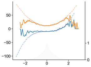
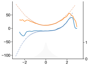
Component Value			Density
	$\mathbf{s}_{1}$	$\mathbf{s}_{1}$

((a)) Marginal effect $\widehat{g_{a}}(\mathbf{s}_{1})$ vs. Monte-Carlo estimate of $U_{1}(\mathbf{s}_{1},a)$.

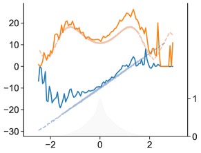
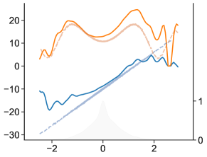
Component Value			Density
	$\mathbf{s}_{2}$	$\mathbf{s}_{2}$

((b)) Marginal effect $\widehat{g_{a}}(\mathbf{s}_{2})$ vs. Monte-Carlo estimate of $U_{2}(\mathbf{s}_{2},a)$.

Figure 4: A comparison of estimated marginal component functions $\widehat{g_{a}}(\mathbf{s}_{i})$ and MC-estimates of $u_{i}(\mathbf{s}_{i},a)$ as described in Section 4.1. For each action, the solid lines represent the estimate of the marginal component function, $g_{a}(\mathbf{s}_{i})$, of $Q^{\pi}(s,a)$ as modeled in Equation 4.4 under a bandwidth of $h=0.001$ (left) and $h=0.01$ (right), while the dashed line represents the Monte-Carlo estimate of $U_{i}(\mathbf{s}_{i},a)$. The observed distribution of the state feature $\mathbf{s}_{i}$ is displayed using the density in grey.

Using $n$ trajectories sampled from this MDP (represented as a batch dataset $\mathcal{D}$), we evaluate the behavioral policy (i.e., $\pi(s^{[i]})=a^{[i]}$) and retrieve the marginal component function $g_{a}(x)$ of the following nonparametric additive model

$$Q^{\pi}(\mathbf{s},a) =g_{a}(\mathbf{s}_{i})+\sum_{j\in[d]/i}f_{j,a}(\mathbf{s}_{j},\mathbf{s}_{i})+\epsilon,$$ (4.4)

where $x=\mathbf{s}_{i}$ and $i\in\{1,2\}$. To measure the performance of our model against a target, we utilize Monte-Carlo (MC) sampling on the MDP to retrieve a direct estimate of the $Q^{\pi_{e}}(s,a)$, evaluated as $\widehat{Q}_{\text{MC}}^{\pi_{e}}(\mathbf{s},a)=\frac{1}{n}\sum_{i=1}^{n}\sum_{j=1}^{\ell}\gamma^{j}r_{ij}$, where $\ell$ is the length of each trajectory and $n$ is the number of sampled trajectories. Since our action-value function is additive, we can similarly construct MC estimates for the component functions $U_{1}(\mathbf{s}_{1},a)$ and $U_{2}(\mathbf{s}_{2},a)$. Lastly, using a pre-specified grid of points $\mathcal{Z}=\{z_{1},\dots,z_{M}\}$, we repeat Algorithm 1 $M$ times to obtain smooth estimates of $g_{a}(\mathbf{s}_{i})$ as described in Section 3.3.

In Figure 4, we observe the nonlinear marginal component functions of the estimated nonparametric additive model represented in Equation (4.4). Under this example, we set the dimensionality of the state space to $d=5$ and the discount factor to $\gamma=0.5$. The dataset $\mathcal{D}$ consisted of 1000 sampled trajectories each with a length of $\ell=10$; the MC estimates were obtained by sampling trajectories of length $\ell$ 100 times. Figure 4 compares the Monte-Carlo estimate of $u_{i}(\mathbf{s}_{i},a)$ to the estimated component function $\widehat{g_{a}}(\mathbf{s}_{i})$ retrieved by the KSH-LSTDQ estimator under a bandwidth of $h=0.001$ and $h=0.01$, respectively. As the bandwidth of the kernel function increases, the model produces a smoother component function since larger weights are assigned to observations further from each local point $z$. Furthermore, note that towards the boundary of the domain, the value of the component function is pulled towards zero. Since, our simulation relies on state transitions sampled from a normal distribution, these regions of the domain generally have fewer observations. As a result, the group Lasso penalty shrinks these sparse regions toward 0. Lastly, while our model, is generally able retrieve the shape of the underlying function at non-sparse regions of the domain, our estimates are also slightly biased for complex functions, as observed for $\widehat{g_{a}}(\mathbf{s}_{2})$.

Mean Regret
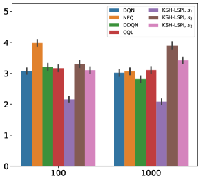
	Number of Episodes

((a)) Dimensionality of $\mathbf{s}_{i}$ is 5.

Mean Regret
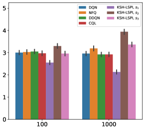
	Number of Episodes

((b)) Dimensionality of $\mathbf{s}_{i}$ is 50.

Figure 5: Regret analysis comparing the performance of KSH-LSPI models, where the candidate feature $x$ is independently represented using state features $\{\mathbf{s}_{1},\mathbf{s}_{2},\mathbf{s}_{3}\}$, and neural network-based approaches as described in Section 4.2. Within each sub-figure, the dimensionality of the state space and the number of episodes used to generate the batch dataset are varied.

4.2 Comparison to Neural Approaches

We evaluate the performance of the KSH-LSPI algorithm against a set of widely-used neural network-based approaches, specifically: neural fitted Q-iteration (NFQ), deep Q-network (DQN), double deep Q-network (DDQN), and conservative Q-learning (CQL) [29, 48, 42, 24]. Each model is trained using a batch dataset of experiences, which are gathered from a random policy interacting in an MDP with correlated state features and an additive reward function. Similar to Equation (4.1), the reward function is dependent on the first two state features $\{\mathbf{s}_{1},\mathbf{s}_{2}\}$ and the selected action $a$. Appendix A.1 provides a detailed description of the MDP and the data generation process. In each experiment, we adjust the dimensionality of the MDP’s state space and the number of episodes used to generate the batch dataset. For the KSH-LSPI algorithm, we fit a separate model, where the candidate feature $x$ is represented as one of the first three state features $\{\mathbf{s}_{1},\mathbf{s}_{2},\mathbf{s}_{3}\}$. Here, each state feature, denoted as $\mathbf{s}_{i}$, contributes to the marginal component, $g_{a}(\mathbf{s}_{i})$, as illustrated in Equation (4.4). We perform policy iteration in accordance with Example 3.1, setting the maximum number of allowed policy iterations to $3$. Detailed specifications and architectures of both the KSH-LSPI models and the neural network-based approaches can be found in Appendix A.2.

Estimated policies from each approach were evaluated within the MDP used to generate the training batch dataset. Specifically, each policy was rolled out for 10 time steps (i.e., an episode), 1000 times. A regret analysis was performed, where, at the end of each episode, the difference between the optimal reward at each time step and the reward obtained by the current policy was calculated. The average of these differences over all episodes was then computed to obtain the estimated mean regret for each experiment. Figure 5 presents results from the regret analysis, where the dimensionality of the state space and the number of episodes used to generate the batch dataset were varied. Within each experiment, we observe that the KSH-LSPI model under a candidate feature of $\mathbf{s}_{2}$ and $\mathbf{s}_{3}$, perform similarly to the neural network-based approaches when the number of episodes is 100, and worse when the number episodes used the generated the batch dataset increases to 1000. Conversely, when $\mathbf{s}_{1}$ (i.e., the feature that accounts for the most variation within the observed rewards) is set as the candidate feature, the KSH-LSPI model outperforms the neural-network based models, and is further improved as the number of episodes increases. These results highlight a key sensitivity in the KSH-LSPI model; that is, the appropriate selection of the candidate feature $x$ largely influences model performance.

5 Motivating Case Study

Postoperative recovery is defined as the period of functional improvement that occurs from the end of surgery and hospital discharge to the instance in which normal function has been restored [6]. Depending on the type of surgery administered, this period of functional recovery can vary drastically and be accompanied by mild to severe complications. For patients who received a corrective surgery for spine disease, post-operative recovery is impacted by the complexity of the diagnosis and surgical procedure received. Additional barriers to recovery for spine disease patients include stress, pain, cognitive dysfunction, and potential postoperative complications [49].

To improve the postoperative recovery and care of spine patients, physicians have employed a multi-pronged approach that focuses on protocols that expedite functional recovery, decrease post-operative complications, and improve subjective patient experience [11]. As part of this effort, patient mobilization and consistent pain management are heavily suggested [7]. To advance theses efforts, physicians require objective measurements of a patient’s functional capacity and pain over the course of their recovery [9, 35, 22, 4]. With respect to spine patients, such measurements can provide a formal understanding and quantification of mobilization activities that expedite overall patient recovery and minimize the risk of complications.

Distance Traveled (km)	Radius of Gyration (km)	Average flight duration (km)
Time Spent at Home (hours)	Maximum Diameter (km)	Fraction of the day spent stationary
Max. Distance from Home (km)	Num. Significant Places Visited	Time Spent Walking
Average flight length (km)	Number of Steps	Average Cadence

Table 1: Subset of GPS and accelerometer-based summary statistics of digital phenotyping. Definitions can be found on the Forest GitHub repository (www.github.com/onnela-lab/forest).

Figure 6: Smoothed mobility proportions (with standard errors represented in grey) for spine disease cohort centered on day of surgery. The lighter shaded area corresponds to the first 30 post-operative days. Receiving a neurosurgical intervention is followed by a period of decreased mobility, where patients tend to travel less and stay at home over a longer duration. Individual-level differences in recovery are driven by factors such as the type of surgery received, the specific diagnosis of spine disease, and patient demographics.

We consider $n=67$ neurosurgical spine patients with median age of 57 years (IQR: 48–65.5) that were enrolled between June 2016 and March 2020 as part of a digital phenotyping study at Brigham and Women’s Hospital. Each patients underwent a neurosurgical intervention in relation to their spine disease. For data collection, patients installed the Beiwe application on their smartphones. Beiwe is a high-throughput research platform that was developed by the Onnela lab at Harvard T.H. Chan School of Public Health for smartphone-based digital phenotyping on iOS and Android devices. Passive features collected on Beiwe includes GPS and accelerometer data in their raw unprocessed form, Bluetooth and WiFi logs, and anonymized phone call and text message logs. Samples were collected from the GPS data stream for 1 minute every 5 minutes, and from the accelerometer data stream for 10 seconds every 10 seconds. Using the raw data sampled from the GPS and accelerometer sensors, a set of behavioral features concerning patient mobility are computed at the daily level [27]. A subset of these features are represented in Table 1. For active data collection, patients were electronically surveyed once daily at 5PM Eastern standard time to evaluate their current pain level. The prompt of the micro-survey was ?Please rate your pain over the last 24 hours on a scale from 0 to 10, where 0 is no pain at all and 10 is the worst pain imaginable.?

Figure 7: Pre- and post-operative pain responses with time centered on the day of surgery (i.e., blue line) with a fitted local regression (i.e., black line) for a random selection of patients. While surgery corresponds to a sharp decline in self-reported pain, we observe a heterogeneous recovery experience among these four patients.

In conjunction with the daily self-reported micro-surveys, these constructed features allow researchers to objectively identify post-operative trends in mobility and pain as it relates to overall functional recovery [4, 9]. To this end, we seek to leverage reinforcement learning to estimate and interpret mobility-based action-value functions that provide recommendations concerning questions such as ?What level of mobilization is advisable after surgery?? and ?How should these levels be adjusted given a patient’s current condition??. The overall goal of these recommendations is to manage a patient’s overall pain level and promote improved recovery. Furthermore, by utilizing an interpretable representation of the estimated action-value function, we seek to identify clinical and digital phenotyping features that are important to consider for decision-making.

6 Application to Surgical Recovery

Using data collected from the spine disease cohort described in Section 5, we implement nonparametric additive models to estimate action-value functions associated with

1. A behavioral policy that aims to mimic decisions commonly taken by patients, and

2. An improved policy retrieved from performing approximate policy iteration on the estimated behavioral policy.

In both cases, the estimated decision-making policy aims to suggest the daily number of steps necessary to reduce long-term ($\gamma\gg 0$) post-operative pain response. We explore both discrete and continuous action spaces and provide a practical interpretation of the additive functional components as presented in Equations (2.6) and (2.7), respectively.

Variable	$n$ $(\%)$ or Median ($25^{\text{th}}$–$75^{\text{th}}$)
Demographic Data
Age	57.0 (48.0–65.5)
Female gender	34 (50.7)
Site of surgery
Cervical	19 (28.4)
Lumbar	27 (40.3)
Thoracic	2 (3.0)
Multiple	18 (26.9)
Data Collection
GPS days of follow-up	61 (49–61)
Accelerometer days of follow-up	61 (50.5–61)
Daily pain survey response rate	59.4 (42.4–76.9)
Digital Phenotypes
Number of places visited	3 (2–5)
Time spent at home (hours)	18.3 (12.9–21.9)
Distance traveled (km)	32.3 (10.8–62.3)
Maximum distance from home (km)	10.6 (4.5–25.5)
Radius of gyration (km)	1.50 (0.18-5.01)
Time spent not moving	21.2 (20.2–22.2)
Average cadence	1.64 (1.55–1.74)
Number of steps	948.6 (356.9–2,005)

Table 2: Participant demographic information and digital phenotyping data for spine disease cohort. Summaries are computed according to the first 60 postoperative days since surgery (including the day of surgery).

6.1 Data Pre-processing

We consider the recovery period of $n=67$ neurosurgical spine disease patients with a mean post-operative follow-up of 87 days (SD = 51.21 days). Baseline clinical information on this study cohort can be found in Table 2. Digital phenotyping features based on raw GPS and accelerometer data were constructed and summarized on a daily time scale to closely monitor each patients’ clinical recovery and/or progression after surgery. These features include passively sampled summary statistics that uniquely describe a patient’s daily mobility and activity levels.

We construct a simple MDP where each time step $t$ corresponds to a day since surgery. The state space, $S\in\mathbb{R}^{d}$ is a multidimensional, continuous state vector that consists of relevant digital phenotyping features and patient-specific demographic information (i.e., age and days since surgery). In total, $d=9$ features were used in this analysis. The action space $\mathcal{A}\in\mathbb{R}$ represents the number of steps taken per day. For the discrete action model, the action space, $\mathcal{A}\in\{0,1\}$, is binarized such that $0$ represents moving less than the subject-level pre-operative median number of steps taken per day and $1$ represents moving above this threshold. The rewards, $r\in\mathbb{R}$, are chosen to be the negative value of the self-reported pain score, where each score is taken from a numerical rating scale between 0 (i.e., no pain) and 10 (i.e., worst pain imaginable). Lastly, we consider a discount factor $\gamma$ of 0.5 to examine estimated policies that aim to reduce long-term pain response.

Under this MDP, we consider up to the first 60 days since surgery for each patient. Patients with a post-operative follow-up period of less than 5 days were excluded. Entries with missing values in either the digital phenotyping features or the daily self-reported pain scores were removed. The batch dataset $\mathcal{D}$ with $N=$ 1,409 daily transitions was constructed using data collected from the study cohort and represented using the MDP. All state features were normalized to [0,1] for model fitting.

6.2 Model Fitting

To estimate the action-value function associated with the behavioral policy $\pi_{b}$, we implement Algorithm 1 where we construct $\bm{\Phi}^{\prime}$ using the observed next-state action contained within each patient-level trajectory in $\mathcal{D}$. That is, $\bm{\Phi}_{i\mathchoice{\mathbin{\vbox{\hbox{\scalebox{0.5}{$\displaystyle\bullet$}}}}}{\mathbin{\vbox{\hbox{\scalebox{0.5}{$\textstyle\bullet$}}}}}{\mathbin{\vbox{\hbox{\scalebox{0.5}{$\scriptstyle\bullet$}}}}}{\mathbin{\vbox{\hbox{\scalebox{0.5}{$\scriptscriptstyle\bullet$}}}}}}^{\prime}=\phi(\mathbf{s}^{{}^{\prime}[i]},a^{[i+1]})$ for the $i^{\text{th}}$ observed transition. Accordingly, the action-value function associated with an improved policy $\pi^{*}$ is estimated by performing approximate policy iteration (as detailed Algorithm 2) on the action-value function associated with the behavioral policy. For both discrete and continuous action versions of the general model (2.4), we use a Gaussian kernel $K(u)=e^{-\frac{1}{2}u^{2}}$ and a grid of evenly-spaced points $\mathcal{Z}$ within a [0,1] range for discretization. For the discrete action model, we estimate the marginal effect $g_{a}(x)$ and the additive joint effects $f_{j,a}(\mathbf{s}_{j},x)$ for $j\geq 2$ for each candidate state feature $x$ in a set $\mathcal{H}$, where $x\neq\mathbf{s}_{j}$.

To select the hyperparameters of the KSH-LSTDQ estimator (i.e., the degree of the B-spline functions, number of basis functions, bandwidth, and regularization penalty), we partitioned the dataset $\mathcal{D}$ into training and validation sets according to a $80\%-20\%$ patient-level split and performed a grid search. Using these partitions, we retrieved a set of hyperparameters that minimized the validation mean squared error between the estimated action-value under the behavioral policy when $\gamma=0$ and the true immediate rewards,

$$\text{MSE}(\mathcal{D}_{\text{Val}})=\frac{1}{|\mathcal{D}_{\text{Val}}|}\sum_{(\mathbf{s},a,r)\sim\mathcal{D}_{\text{Val}}}\Big{(}\widehat{Q}^{\pi_{b}}(\mathbf{s},a)-r\Big{)}^{2}.$$

Accordingly, these hyperparameters were used to retrieve the KSH-LSTDQ estimators for MDPs where $\gamma$ is set to 0.5. The set of hyperparameters used for each estimated model is displayed in Appendix B.1.

6.3 Results and interpretations

We visualize and interpret the estimated the additive component functions of the action-value functions associated with the behavioral and improved policies.

6.3.1 Discrete Action Model

For the discrete action model, we model a nonparametric action-value function for each candidate state feature in the set $\mathcal{H}$, which we represent as $x$. Here, $\mathcal{H}$ consists of the following features: age, number of days since surgery, time spent at home (hours), and distance traveled (km).

Marginal State Feature Effects. In Figure 8, we examine the marginal effect $\widehat{g}_{a}(x)$ of the estimated action-value function for each candidate state feature $x\in\mathcal{H}$ under the behavioral policy $\pi_{b}$ and the improved policy $\pi^{*}$ constructed using policy iteration. Specifically, $\widehat{g}_{a}(x)$ returns the estimated marginal change in long-term negative pain response for a given state feature $x$ under action $a$. Across each sub-figure in Figure 8(a), moving above a patient’s pre-operative baseline number of steps ($a=1$) within a given day is associated with a higher immediate negative pain response in comparison to the converse action ($a=0$), regardless of the value of $x$. This observation is inline with clinical research that suggests movement at or above a patient’s pre-operative baseline is associated with improved post-operative functional recovery [10, 33, 33, 9].

Within each select action, the marginal effect shows a nonlinear change in long-term pain response. When $x=\text{{age}}$, Figure 8(a) suggests a marginal increase in long-term negative pain response for small and large values of age. This observation supports clinical studies suggesting the existence of age-related pain sensitivity that peaks during mid-life [52]. Additionally, when $x=\text{{time spent at home}}$, our model suggests that spending more time at home is associated with a nonlinear decrease in negative pain response. Furthermore, when $x=\text{{distance traveled}}$, we observe that, regardless of the selected action, traveling less than $150$km is associated with a constant effect on negative pain response, whereas traveling beyond $150$km within a given day is associated with an increasing effect. We note that this association is possibly due to survivorship bias present in the model estimates, where a few patients report minimal pain during periods of excessive travel.

Lastly, when $x=\text{{days since surgery}}$, our model examines the impact of mobilization as the number of days since surgery increases. We note the difference in the marginal effect among both actions is maximized for days closest to the onset of surgery, suggesting that increased mobilization during early periods of recovery may be associated with decreased pain response. This finding supports current clinical practice that suggests early mobilization enhances surgical recovery, a cornerstone of post-operative pain management [49, 7].

The differences between the marginal effects associated with the behavioral and improved policies, as shown in Figure 8(b), are subtle. While the underlying trends and ordering of actions are relatively consistent, the estimated effect sizes appear to be smaller for select candidate state features under the improved policy (e.g., $x=$ age, time spent at home, or days since surgery) compared to those of the behavioral policy.

Move ABOVE preoperative baseline ($a=1$):      Move BELOW preoperative baseline ($a=0$):  

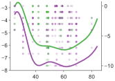
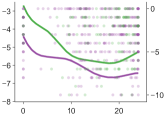
Marginal Effect			Negative Pain Score
	$x=\text{Age}$	$x=\text{Time spent at home (hours)}$
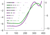
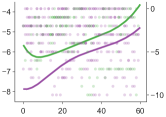
Marginal Effect			Negative Pain Score
	$x=\text{Distance traveled (km)}$	$x=\text{Days since surgery}$

((a)) Behavioral policy

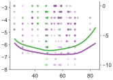
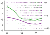
Marginal Effect			Negative Pain Score
	$x=\text{Age}$	$x=\text{Time spent at home (hours)}$
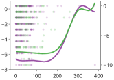
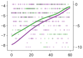
Marginal Effect			Negative Pain Score
	$x=\text{Distance traveled (km)}$	$x=\text{Days since surgery}$

((b)) Policy Iteration

Figure 8: A comparison of the marginal component function $\widehat{g}_{a}(x)$ of $Q^{\pi}(\mathbf{s},a,x)$ estimated under the behavioral policy $\pi=\pi_{b}$ vs. the improved policy $\pi=\pi^{*}$. Each sub-figure is associated with a separate nonparametric additive model of $Q^{\pi}(\mathbf{s},a,x)$, where the state feature representing $x$ is changed. For each action, the solid lines represent the estimate of the marginal component function $\widehat{g}_{a}(x)$ over the range of observed values of $x$, whereas the points represent the value of the associated observed rewards (i.e., negative pain score) over $x$.

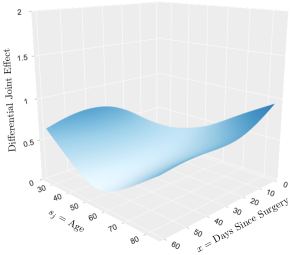
((a)) Behavioral policy

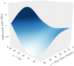
((b)) Policy Iteration

Figure 9: Surface plots representing the difference between the joint component functions $\widehat{f}_{j,1}(\mathbf{s}_{j},x)$ and $\widehat{f}_{j,0}(\mathbf{s}_{j},x)$ (i.e., the differential benefit of selecting action $a$=1 over $a=0$) of $Q^{\pi}(\mathbf{s},a,x)$ estimated under the behavioral policy $\pi=\pi_{b}$ vs. the improved policy $\pi=\pi^{*}$.

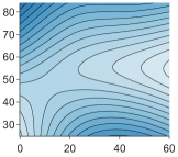
Age		Time spent not moving
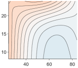
$x=\text{Days since surgery}$		$x=\text{Age}$
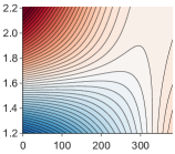
Average Cadence		Max. dist. from home
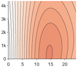
$x=\text{Distance travel}$		$x=\text{Time spent at home}$

((a)) Behavioral policy

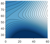
Age		Time spent not moving
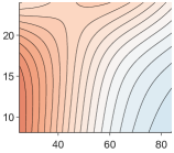
$x=\text{Days since surgery}$		$x=\text{Age}$
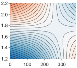
Average Cadence		Max. dist. from home
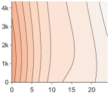
$x=\text{Distance travel}$		$x=\text{Time spent at home}$

((b)) Policy Iteration

Figure 10: Contour plots representing the differential benefit of selecting action $a=1$ over $a=0$ with respect to joint effects $\widehat{f}_{j,a}(\mathbf{s}_{j},x)$ under $Q^{\pi}(\mathbf{s},a,x)$ estimated under the behavioral policy $\pi=\pi_{b}$ vs. the improved policy $\pi=\pi^{*}$. Each sub-figure is associated with a separate nonparametric additive model of $Q^{\pi}(\mathbf{s},a,x)$, where the state feature representing $x$ is changed.

Joint Effects betwen State Features. In Figures 10 and 10, we examine the joint effect $f_{j,a}(x,\mathbf{s}_{j})$ of the estimated action-value function between select state features $\mathbf{s}_{j}$ (i.e., age, time spent not moving, average cadence, and maximum distance from home) and candidate state features $x\in\mathcal{H}$. The value of each joint feature pair corresponds to a nonlinear effect on an estimated smooth surface representing the additive, long-term change in negative pain response. We specifically examine the benefit of selecting a given action over its converse by visualizing the difference between the joint effects under both actions, i.e., $f_{j,1}-f_{j,0}$. Differences greater than zero indicate an additive preference for action $a=1$, over the converse $a=0$.

When examining the joint effect between $x=\text{{days since surgery}}$ and $\mathbf{s}_{j}=\text{{age}}$, we observe that regardless of the value of each corresponding feature, moving more than the pre-operative baseline is associated with an increase in negative pain response throughout the domain of the joint component function. Interestingly, this association is more pronounced among younger patients under the improved policy. This observation is consistent with clinical research suggesting a relationship between increased post-operative movement and improved rehabilitation, and its potential modification by factors such as age [33, 10, 21].

When $x=\text{{distance traveled}}$ and $\mathbf{s}_{j}=\text{{average cadence}}$, maintaining a slower average walking cadence over longer distances seems to be associated with moving beyond the pre-operative baseline step count. This association is relatively consistent across both the behavioral and improved policies. However, under the improved policy, a positive association is noticed with faster walking cadences near the upper boundary of total distance traveled. In general, the differential relationship between $x=\text{{distance traveled}}$ and $\mathbf{s}_{j}=\text{{average cadence}}$ could be indicative of the shift from automaticity to executive control of locomotion, as seen in rehabilitation literature [8]. This shift may occur as distances increase or as walking becomes more challenging (e.g., due to physical exertion, elevated pain response, or injury), requiring individuals to expend more cognitive effort (i.e., executive control) to manage their gait.

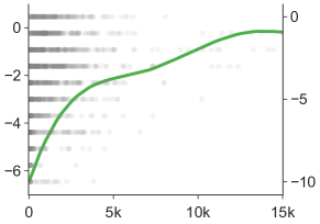
Marginal Effect		Negative Pain Score
	$a=\text{Step count}$

((a)) Behavioral policy

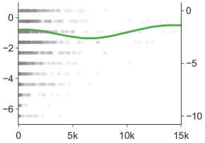
Marginal Effect		Negative Pain Score
	$a=\text{Step count}$

((b)) Policy Iteration

Figure 11: The marginal component function $\widehat{g}(a)$ of $Q^{\pi}(\mathbf{s},a)$ estimated under the behavioral policy $\pi=\pi_{b}$ vs. the improved policy $\pi=\pi^{*}$. The solid lines represent the estimate of the marginal component function $\widehat{g}(a)$ over the observed values $a$, whereas the points represent the value of the associated observed reward (i.e., negative pain score).

6.3.2 Continuous Action Model

We estimate a nonparametric action-value function for a continuous action (i.e., number of steps taken) under the behavioral and improved policies.

Marginal effects. In Figure 11, we examine the marginal effect $\widehat{g}(a)$ of the estimated action-value function. Specifically, $\widehat{g}(a)$ returns the estimated change in long-term negative pain score for a select value of $a$, or number of steps taken. Similar to the discrete action model, the marginal effect of the continuous action reveals a positive association between number of steps taken and long-term negative pain response, especially under the behavioral policy. For the behavioral policy (as shown in Figure 11(a)), we observe that the marginal effect is log-shaped and increases with number of steps taken. On the other hand, for the improved policy (as shown in Figure 11(b)), we observe that the marginal effect of the improved policy is relatively constant across the observed number of steps taken.

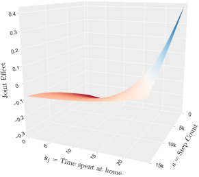
((a)) Behavioral policy

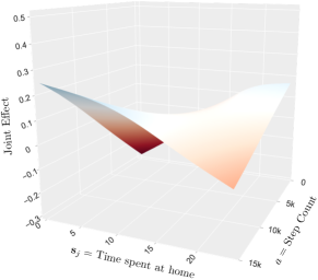
((b)) Policy Iteration

Figure 12: Surface plots representing the joint component functions $\widehat{f}_{j}(\mathbf{s}_{j},a)$ of $Q^{\pi}(\mathbf{s},a)$ estimated under the behavioral policy $\pi=\pi_{b}$ vs. the improved policy $\pi=\pi^{*}$.

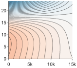
Time spent at home		Distance traveled
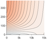
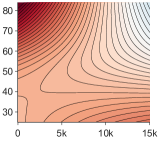
Age		Days since surgery
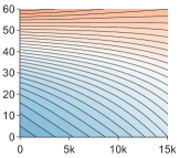
$a=\text{Step count}$		$a=\text{Step count}$

((a)) Behavioral policy

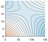
Time spent at home		Distance traveled
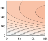
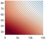
Age		Days since surgery
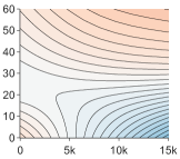
$a=\text{Step count}$		$a=\text{Step count}$

((b)) Policy Iteration

Figure 13: Contour plots representing the joint component functions $\widehat{f}_{j}(\mathbf{s}_{j},a)$ of $Q^{\pi}(\mathbf{s},a)$ estimated under the behavioral policy $\pi=\pi_{b}$ vs. the improved policy $\pi=\pi^{*}$. Each sub-figure is associated with the same nonparametric additive model, but represents a different state feature $\mathbf{s}_{j}$ on the y-axis.

Joint effects between State Features and Actions. In Figures 13 and 13, we examine the joint effects $\widehat{f}_{j}(\mathbf{s}_{j},a)$ between select state features $\mathbf{s}_{j}$ and the continuous action $a$ of the estimated action-value functions. When $a=\text{{step count}}$ and $\mathbf{s}=\text{{time spent at home}}$, we observed that increased time spent at home beyond 15 hours is associated with a positive increase in negative pain response across observed values of step count under the behavioral policy. This trend changes under the improved policy, where joint effect is maximized when step count increases and time spent at home increases and when step count is minimized and time spent at home increases.

Similar to the discrete action model, we observe a differential change in the joint effect associated with age. Under the behavioral and improved policy, an increase in step count across age is relatively associated with an increase the negative pain response.

7 Discussion

In this study, we introduced a regularized, nonparametric additive model for action-value function representation. Our approach, KSH-LSPI, distinguishes itself from LSPI by avoiding parametric assumptions about the action-value function’s form. It achieves this by incorporating ideas directly from local kernel regression and spline methods. This estimation approach affords KSH-LSPI the ability to capture the nonlinear additive contribution of each state-action feature represented in the model. Furthermore, by introducing a group Lasso penalty to our primary objective function, we perform component-wise variable selection and retrieve a parsimonious representation of the action-value function.

In the simulation study, we evaluate the performance of the proposed estimator and examine its sensitivity to changes in its hyperparameters. Future work aims to delve deeper, examining the estimator’s finite sample properties both theoretically and through further simulations. The application of the proposed method to the digital phenotyping spine disease dataset also provides new insights into mobilization behaviors that support post-operative pain management and reaffirmed several well-studied clinical findings. In future applications to spine disease recovery, we hope to extend the model by including categorical features such as gender, race, and diagnosis, as well as additional clinical features such as medication use.

However, this study is not without limitations. Outcomes from our model require careful interpretation and should not be deemed significant without comprehensive uncertainty quantification. In future adaptations of the KSH-LSPI model, we hope to formalize our uncertainty concerning our model estimates by incorporating a form of interval estimation. In the offline reinforcement learning setting, uncertainty-based approaches have shown promise in offline RL by prioritizing risk adverse policies when performing policy improvement [44, 31, 15]. This naturally brings light to a limitation concerning our method’s approach for policy improvement. After evaluating the current policy using KSH-LSTDQ, our policy improvement step greedily selects actions that maximize the estimated action-value function. Unfortunately, function approximation methods in offline reinforcement learning are prone to providing overly optimistic values for state-action pairs that are unobserved in the training data. Hence, safe policy improvement steps, within the actor-critic framework, that regularize the learned policy toward the behavioral policy is encouraged in offline reinforcement learning, especially in healthcare applications [50]. Another potential remedy would be to initialize our algorithm using an initial policy that closely reflects behaviors that would be suggested by a clinical expert. Initialization using physician guided policies helps prevent the algorithm from becoming overly optimistic by selecting best actions that physicians themselves may select [16].

The push for interpretability in machine learning models, especially within healthcare contexts, is driven by a need for transparency in decision-making processes. Compared to the powerful, but often less interpretable neural network methodologies, nonparametric additive models for value-functions offers a representation where decision-making policies can be understood and scrutinized. Such interpretability is essential for potential clinical applications, given the need for clinicians to trust and validate the recommendations derived from these models. In conclusion, the KSH-LSPI model, while having areas that require further refinement, provides a promising framework that aligns with the demand for both efficacy and transparency.

Appendix A Simulation Study

A.1 MDP with Correlated States and Additive Rewards

We consider a multidimensional, continuous state MDP with binary actions and an additive reward function. For each sampled trajectory, elements of the initial state vector $\mathbf{s}^{(0)}\in\mathbb{R}^{d}$ are sampled as $\mathbf{s}^{(0)}_{i}\in$ Uniform[0,1] for all $i\in[d]$. At each time step $t$, we randomly sample an action $a^{(t)}\in\{0,1\}$ with probability $\frac{1}{2}$. State transitions for each state feature are determined by following the equation:

$$\mathbf{s}_{i}^{(t+1)}=\frac{X_{i}^{(t)}+b\hskip 2.0ptU}{1+b}+\delta\hskip 2.0pt\mathbf{s}_{i}^{(t)}+\epsilon_{i},$$ (A.1)

where $X_{i}^{(t)}$ and $U$ follow Uniform[0,2] and Uniform[0,1], respectively, and $\epsilon_{i}\sim\mathcal{N}(0,0.3)$. Furthermore, we set $b$ and $\delta$ to 0.1. When the action $a$ is 0, the signs of the state components change, and otherwise remain the same when $a$ is 1. Under this MDP, we construct a reward function:

$$r(\mathbf{s},a)=u_{1}(\mathbf{s}_{1},a)+u_{2}(\mathbf{s}_{2},a)$$ (A.2)

with reward components that are reliant only on the state features $\mathbf{s}_{1}$ and $\mathbf{s}_{2}$, where:

$$u_{1}(\mathbf{s}_{1},a) =(4\mathbf{s}_{1}-5)\mathbb{1}(a=1)-(5\mathbf{s}_{1}^{2}+5)\mathbb{1}(a=0)$$ (A.3)

$$u_{2}(\mathbf{s}_{2},a) =(\sin(\mathbf{s}_{2}^{2})+5)\mathbb{1}(a=1)+(2\mathbf{s}_{3}-5)\mathbb{1}(a=0)$$ (A.4)

and $g_{j}(\mathbf{s}_{j},a)=0$ for all $j\geq 3$.

A.2 Model Specification and Architecture

A.2.1 Neural Network Approaches

Each neural network-based approach (i.e., DQN, DDQN, NFQ, and CQL) uses the same common architecture to represent their policy and/or value function. Specifically, the input layer is followed by two subsequent dense layers with 64 hidden units each. Each hidden unit leverages a rectified linear unit (ReLU) activation function. Each method was trained over a span of 20 epochs, with each epoch consisting 100 steps and a batch size of 256. For DQN and DDQN, the target network is updated after 500 iterations. The learning rates of DQN, DDQN and NFQ were set to $6.25\times 10^{-5}$, whereas the learning rates of the policy and value network of CQl were set to 0.0001 and 0.0003, respectively.

A.2.2 KSH-LSPI Model

For each experiment, the hyper-parameters of each nonparametric additive model were identical. The bandwidth $h$ was set to 0.001. Each feature was represented as a linear combination of 5 B-spline basis functions with a degree of 2. The regularization parameter $\lambda$ was set to 5, while the learning rate $\mu$ was set to 0.001. We use a grid of 100 local points within a [0,1] range to represent $Q^{\pi}(\mathbf{s},a,\cdot)$. The maximum allowable number of iterations for Algorithm 1 is 500, while the number of policy iterations in Algorithm 2 is 3.

Appendix B Application to Surgical Recovery

B.1 Model Hyperparameters

Model Type	Candidate Feature	Degree	$h$	$\lambda$	$\mu$	$\#$ of Local Points	$\#$ of Basis Functions
Discrete action
Behavioral	Days since surgery	3	0.05	0	0.0001	100	10
Behavioral	Age	3	0.05	0	0.0001	100	10
Behavioral	Distance traveled	3	0.05	1	0.0001	100	10
Behavioral	Time spent at home	3	0.05	0	0.0001	100	10
Improved	Days since surgery	3	0.05	0	0.0001	100	10
Improved	Age	3	0.05	0	0.0001	100	10
Improved	Distance traveled	3	0.05	1	0.0001	100	10
Improved	Time spent at home	3	0.05	0	0.0001	100	10
Continuous action
Behavioral	Step count	3	0.001	1	0.0001	20	10
Improved	Step count	3	0.001	1	0.0001	20	10

Table 3: A summary of the model type and associated parameters utilized in the KSH-LSPI models.

References

- [1] Inkyung Ahn and Jooyoung Park “Drug scheduling of cancer chemotherapy based on natural actor-critic approach” In Bio Systems 106.2-3 Biosystems, 2011, pp. 121–129 DOI: 10.1016/J.BIOSYSTEMS.2011.07.005
- [2] András Antos, Csaba Szepesvári and Rémi Munos “Fitted Q-iteration in continuous action-space MDPs” In Advances in Neural Information Processing Systems 20.1, 2007 URL: http://hal.inria.fr/inria-00185311/en/.
- [3] Dimitri P Bertsekas “Approximate policy iteration: a survey and some new methods” In J Control Theory Appl 9.3, 2011, pp. 310–335 DOI: 10.1007/s11768-011-1005-3
- [4] Alessandro Boaro, Harrison T Reeder and Francesca Siddi “Smartphone GPS signatures of patients undergoing spine surgery correlate with mobility and current gold standard outcome measures Digital Phenotyping in Neurosurgery View project Intracranial aneurysm View project” In Article in Journal of neurosurgery. Spine, 2021 DOI: 10.3171/2021.2.SPINE202181
- [5] Melanie K. Bothe et al. “The use of reinforcement learning algorithms to meet the challenges of an artificial pancreas” In Expert review of medical devices 10.5 Expert Rev Med Devices, 2013, pp. 661–673 DOI: 10.1586/17434440.2013.827515
- [6] A. J. Bowyer and C. F. Royse “Postoperative recovery and outcomes – what are we measuring and for whom?” In Anaesthesia 71 John Wiley & Sons, Ltd, 2016, pp. 72–77 DOI: 10.1111/ANAE.13312
- [7] Burgess and Wainwright “What Is the Evidence for Early Mobilisation in Elective Spine Surgery? A Narrative Review” In Healthcare 7.3 MDPI AG, 2019, pp. 92 DOI: 10.3390/healthcare7030092
- [8] David J Clark “Automaticity of walking: functional significance, mechanisms, measurement and rehabilitation strategies.” In Frontiers in human neuroscience 9, 2015, pp. 246 DOI: 10.3389/fnhum.2015.00246
- [9] David J Cote, Ian Barnett, Jukka Pekka Onnela and Timothy R Smith “Digital Phenotyping in Patients with Spine Disease: A Novel Approach to Quantifying Mobility and Quality of Life” In World Neurosurgery 126 Elsevier Inc., 2019, pp. e241–e249 DOI: 10.1016/j.wneu.2019.01.297
- [10] C Duc et al. “Objective evaluation of cervical spine mobility after surgery during free-living activity.” In Clinical biomechanics (Bristol, Avon) 28.4, 2013, pp. 364–369 DOI: 10.1016/j.clinbiomech.2013.03.006
- [11] Mazin Elsarrag et al. “Enhanced recovery after spine surgery: A systematic review” In Neurosurgical Focus 46.4, 2019, pp. 1–8 DOI: 10.3171/2019.1.FOCUS18700
- [12] Jianqing Fan and Jiancheng Jiang “Nonparametric inferences for additive models” In Journal of the American Statistical Association 100.471 Taylor & Francis, 2005, pp. 890–907 DOI: 10.1198/016214504000001439
- [13] Amir-massoud Farahmand et al. “Regularized Policy Iteration with Nonparametric Function Spaces” In Journal of Machine Learning Research 17, 2016, pp. 1–66
- [14] Matthieu Geist and Bruno Scherrer “l1-penalized projected Bellman residual” In European Wrokshop on Reinforcement Learning, 2011 URL: https://hal.inria.fr/hal-00644507
- [15] Mohammad Ghavamzadeh, Shie Mannor, Joelle Pineau and Aviv Tamar “Bayesian Reinforcement Learning: A Survey” In Foundations and Trends in Machine Learning 8.5-6 Now Publishers Inc, 2016, pp. 359–483 DOI: 10.1561/2200000049
- [16] Omer Gottesman et al. “Guidelines for reinforcement learning in healthcare” In NAture MediciNe — 25, 2019, pp. 14–18 DOI: 10.1038/s41591-018-0310-5
- [17] Trevor J. Hastie “Generalized Additive Models” In Statistical Models in S Routledge, 2017, pp. 249–307 DOI: 10.1201/9780203738535-7
- [18] Matthew W. Hoffman, Alessandro Lazaric, Mohammad Ghavamzadeh and Rémi Munos “Regularized least squares temporal difference learning with nested L2 and L1 penalization” In Lecture Notes in Computer Science (including subseries Lecture Notes in Artificial Intelligence and Lecture Notes in Bioinformatics) 7188 LNAI, 2012, pp. 102–114 DOI: 10.1007/978-3-642-29946-9–“˙˝13
- [19] Matthew Howard and Yoshihiko Nakamura “Locally weighted least squares policy iteration for model-free learning in uncertain environments” In IEEE International Conference on Intelligent Robots and Systems, 2013, pp. 1223–1229 DOI: 10.1109/IROS.2013.6696506
- [20] Ronald A. Howard “Dynamic programming and Markov processes” John Wiley, 1960 URL: https://psycnet.apa.org/record/1961-01474-000
- [21] Maria Jaensson, Karuna Dahlberg and Ulrica Nilsson “Factors influencing day surgery patients’ quality of postoperative recovery and satisfaction with recovery: a narrative review” In Perioperative Medicine 8.1, 2019, pp. 3 DOI: 10.1186/s13741-019-0115-1
- [22] Marta Karas et al. “Predicting Subjective Recovery from Lower Limb Surgery Using Consumer Wearables” In Digital Biomarkers 4.1 Karger Publishers, 2020, pp. 73–86 DOI: 10.1159/000511531
- [23] J Zico Kolter and Andrew Y Ng “Regularization and feature selection in least-squares temporal difference learning” In ACM International Conference Proceeding Series 382, 2009 DOI: 10.1145/1553374.1553442
- [24] Aviral Kumar, Aurick Zhou, George Tucker and Sergey Levine “Conservative Q-Learning for Offline Reinforcement Learning” In Advances in Neural Information Processing Systems 2020-Decem Neural information processing systems foundation, 2020 DOI: 10.48550/arxiv.2006.04779
- [25] John Lafferty and Larry Wasserman “Rodeo: Sparse, greedy nonparametric regression” In Annals of Statistics 36.1, 2008, pp. 28–63 DOI: 10.1214/009053607000000811
- [26] Michail G. Lagoudakis and Ronald Parr “Least-squares policy iteration” In Journal of Machine Learning Research 4.6, 2004, pp. 1107–1149 DOI: 10.1162/1532443041827907
- [27] Gang Liu and Jukka Pekka Onnela “Bidirectional imputation of spatial GPS trajectories with missingness using sparse online Gaussian Process” In Journal of the American Medical Informatics Association 28.8 Oxford Academic, 2021, pp. 1777–1784 DOI: 10.1093/JAMIA/OCAB069
- [28] Junwei Lu, Mladen Kolar and Han Liu “Kernel Meets Sieve: Post-Regularization Confidence Bands for Sparse Additive Model” In Journal of the American Statistical Association 115.532, 2020, pp. 2084–2099 DOI: 10.1080/01621459.2019.1689984
- [29] Volodymyr Mnih et al. “Playing Atari with Deep Reinforcement Learning”, 2013 DOI: 10.48550/arxiv.1312.5602
- [30] Volodymyr Mnih et al. “Human-level control through deep reinforcement learning” In Nature 518.7540 Nature Publishing Group, 2015, pp. 529–533 DOI: 10.1038/NATURE14236
- [31] Brendan O’Donoghue, Ian Osband, Remi Munos and Volodymyr Mnih “The Uncertainty Bellman Equation and Exploration” In 35th International Conference on Machine Learning, ICML 2018 9 International Machine Learning Society (IMLS), 2017, pp. 6154–6173 URL: https://arxiv.org/abs/1709.05380v4
- [32] Jukka-Pekka Onnela “Opportunities and challenges in the collection and analysis of digital phenotyping data” In Neuropsychopharmacology, 2020 DOI: 10.1038/s41386-020-0771-3
- [33] Gulsah Ogutluler Ozkara et al. “Effectiveness of physical therapy and rehabilitation programs starting immediately after lumbar disc surgery.” In Turkish neurosurgery 25.3, 2015, pp. 372–379 DOI: 10.5137/1019-5149.JTN.8440-13.0
- [34] Regina Padmanabhan, Nader Meskin and Wassim M. Haddad “Closed-loop control of anesthesia and mean arterial pressure using reinforcement learning” In Biomedical Signal Processing and Control 22 Elsevier, 2015, pp. 54–64 DOI: 10.1016/J.BSPC.2015.05.013
- [35] Nikhil Panda et al. “Smartphone Global Positioning System (GPS) Data Enhances Recovery Assessment After Breast Cancer Surgery” In Annals of Surgical Oncology, 2020 DOI: 10.1245/s10434-020-09004-5
- [36] Nikhil Panda et al. “Using Smartphones to Capture Novel Recovery Metrics after Cancer Surgery” In JAMA Surgery 155.2, 2020, pp. 123–129 DOI: 10.1001/jamasurg.2019.4702
- [37] Xuefeng Peng et al. “Improving Sepsis Treatment Strategies by Combining Deep and Kernel-Based Reinforcement Learning” In AMIA Annual Symposium Proceedings 2018 American Medical Informatics Association, 2018, pp. 887 URL: /pmc/articles/PMC6371300//pmc/articles/PMC6371300/?report=abstracthttps://www.ncbi.nlm.nih.gov/pmc/articles/PMC6371300/
- [38] Thomas Peyser, Eyal Dassau, Marc Breton and Jay S. Skyler “The artificial pancreas: current status and future prospects in the management of diabetes” In Annals of the New York Academy of Sciences 1311.1 Ann N Y Acad Sci, 2014, pp. 102–123 DOI: 10.1111/NYAS.12431
- [39] Aniruddh Raghu et al. “Continuous State-Space Models for Optimal Sepsis Treatment - a Deep Reinforcement Learning Approach”, 2017, pp. 1–17 URL: http://arxiv.org/abs/1705.08422
- [40] Pradeep Ravikumar, John Lafferty, Han Liu and Larry Wasserman “Sparse Additive Models” In Journal of the Royal Statistical Society. Series B: Statistical Methodology 71.5, 2007, pp. 1009–1030 URL: http://arxiv.org/abs/0711.4555
- [41] Peter Richtárik and Martin Takáč “Iteration complexity of randomized block-coordinate descent methods for minimizing a composite function” In Mathematical Programming 144.1-2, 2014, pp. 1–38 DOI: 10.1007/s10107-012-0614-z
- [42] Martin Riedmiller “Neural fitted Q iteration - First experiences with a data efficient neural Reinforcement Learning method” In Lecture Notes in Computer Science (including subseries Lecture Notes in Artificial Intelligence and Lecture Notes in Bioinformatics) 3720 LNAI Springer, Berlin, Heidelberg, 2005, pp. 317–328 DOI: 10.1007/11564096–“˙˝32/COVER
- [43] Eric D. Sinzinger and Brett Moore “Sedation of Simulated Icu Patients Using Reinforcement Learning Based Control” In International Journal on Artificial Intelligence Tools 14.1-2 World Scientific Publishing Company, 2011, pp. 137–156 DOI: 10.1142/S021821300500203X
- [44] Aaron Sonabend-W et al. “Expert-Supervised Reinforcement Learning for Offline Policy Learning and Evaluation” In Advances in Neural Information Processing Systems 2020-December Neural information processing systems foundation, 2020 URL: https://arxiv.org/abs/2006.13189v2
- [45] Richard S. Sutton and Andrew G. Barto “Reinforcement Learning, Second Edition: An Introduction - Complete Draft” In The MIT Press, 2018, pp. 1–3 URL: https://mitpress.mit.edu/books/reinforcement-learning-second-edition
- [46] John Torous, Patrick Staples and Jukka Pekka Onnela “Realizing the Potential of Mobile Mental Health: New Methods for New Data in Psychiatry” In Current Psychiatry Reports 17.8 Current Medicine Group LLC 1, 2015, pp. 1–7 DOI: 10.1007/s11920-015-0602-0
- [47] Nikolaos Tziortziotis and Christos Dimitrakakis “Bayesian Inference for Least Squares Temporal Difference Regularization”, 2017, pp. 1593212 URL: https://hal.inria.fr/hal-01593212
- [48] Hado Van Hasselt “Double Q-learning” In Advances in Neural Information Processing Systems 23, 2010
- [49] Thomas W Wainwright, Tikki Immins and Robert G Middleton “Enhanced recovery after surgery (ERAS) and its applicability for major spine surgery” In Best Practice and Research: Clinical Anaesthesiology 30.1 Elsevier Ltd, 2016, pp. 91–102 DOI: 10.1016/j.bpa.2015.11.001
- [50] Ziyu Wang et al. “Critic Regularized Regression” In Advances in Neural Information Processing Systems 2020-December Neural information processing systems foundation, 2020 URL: https://arxiv.org/abs/2006.15134v3
- [51] Xin Xu, Dewen Hu and Xicheng Lu “Kernel-based least squares policy iteration for reinforcement learning” In IEEE Transactions on Neural Networks 18.4, 2007, pp. 973–992 DOI: 10.1109/TNN.2007.899161
- [52] Robert P Yezierski “The effects of age on pain sensitivity: preclinical studies.” In Pain medicine (Malden, Mass.) 13 Suppl 2.Suppl 2, 2012, pp. 27–36 DOI: 10.1111/j.1526-4637.2011.01311.x