JISA: A Polymorphic Test-and-Measurement Automation Library

Abstract

JISA is a software library, written in Java, aimed at providing an easy, flexible and standardised means of creating experimental control software for physical sciences researchers. Specifically, with an emphasis on enabling measurement code to be written in an instrument-agnostic way, allowing such routines to be reused across multiple different setups without requiring modification. Additionally, it provides a simple means of recording and handling data, as well as pre-built graphical user interface (GUI) “blocks” to enable the relatively easy creation of graphical control systems. Together these allow users to quickly piece together test-and-measurement programs with coherent user interfaces, without requiring much experience of such things.

Nr.	Code metadata description
C1	Current code version	1.0
C2	Permanent link to code/repository used for this code version	https://github.com/OE-FET/JISA
C3	Code capsule	N/A
C4	Legal Code License	AGPLv3
C5	Code versioning system used	git
C6	Software code languages, tools, and services used	Java
C7	Compilation requirements, operating environments and dependencies	JDK 11 or newer
C8	Developer documentation/manual	https://github.com/OE-FET/JISA/wiki
C9	Support email for questions	waw31@cam.ac.uk

Table 1: Code metadata.

1 Introduction and Motivation

Writing software to control experimental systems, where multiple, individual instruments are made to work in concert to perform automated measurement routines, is commonplace in physical sciences research. When considering how such software controls each instrument, one can split the process into three parts. The first of these is the instrument itself, which listens to instructions sent to it from the controlling computer — often responding by taking some action and/or replying [1, 2, 3]. The second is the “driver”, the software library used to format and send these commands over some hardware protocol and interpret responses from the instrument. The main purpose of this is to present the functionality of the instrument, as well as any output it may give, in a way that is readily useable by a programmer. The third part we shall label the “routine”, where the logic of a measurement is laid out. This is essentially the software that makes use of the driver to control the instrument as part of some wider measurement routine. Boundaries between entities (such as those listed here) and how information flows through them, are referred to as “interfaces” in computer science [4]. Therefore, there are two interfaces in this picture: Instrument $\leftrightarrow$ Driver (ID), and Driver $\leftrightarrow$ Routine (DR).

For instruments, their ID interfaces are defined by their manufacturer, almost always with some degree of arbitrariness. As a result, two instruments with the same functionality, but of different make and model, are unlikely to have compatible ID interfaces, and thus will require different drivers. Furthermore, because drivers, and thus DR interfaces, are normally designed to follow the same rough structure as the ID interface of their target instrument, the same incompatibility often applies to DR interfaces too. The result of this is that a routine written to perform an experiment using one set of instruments would need to be significantly altered to accommodate instruments of the same type, but different makes and models, thus often preventing measurement code from being reusable.

As an illustrative example, let us suppose we have two voltmeters: A and B. Voltmeter A holds the settings of measurement range, “rng”, and integration time, “time”, persistently in its own memory, which it recalls whenever it is instructed to take a measurement. Voltmeter B, on the other hand, treats the task more like a one-off spot measurement, with both parameters needing to be specified in the measurement command each time. If drivers were to be written for these instruments, with their DR interfaces made to mimic the ID interfaces defined above, then they will look drastically different. The driver for A will have three methods, two for individually setting the rng and time settings, and one for triggering a measurement, whereas B will only have one method which takes both rng and time as arguments. This is depicted in the top row of Figure 1.

Figure 1: Diagrammatic representations of the ID and DR interfaces for two instruments, A and B, where the methods exposed by the driver to the measurement routine are represented as information sent from the routine to the driver over the DR interfaces, where they are converted into the specific command codes required by the instrument, and then sent to the instrument over the ID interface. The top row represents a typical DR interface made to simply mimic the ID interface, whereas the bottom row shows how both instruments could be abstracted behind a common interface allowing interchangeability.

Clearly, any measurement routine using the driver for A would require significant alteration to instead accommodate B. However, this can be avoided by defining a common interface, and hiding the differences in the underlying implementation behind it. For instance, the rng and time settings for B could be held as variables within the driver layer, with them being recalled and sent any time a voltage measurement is requested (as well as holding initial default values). That way, both A and B can implement a common DR interface, as is shown on the bottom row of Figure 1. Now, a measurement routine can be written that will work regardless of whether it is using A or B as, from the perspective of the routine, they are now indistinguishable. In essence, we have taken the concept of a voltmeter, and turned it into a black box by defining a common voltmeter interface. In rough terms, this is what is known as “polymorphism” in object-oriented programming: where one has multiple, interchangeable objects of different classes that all implement the same interface.

Most available tools and drivers tend to lack any such standardisation. For instance, in National Instruments’ LabVIEW, instrument drivers are typically written in a completely procedural manner, using no object-oriented features at all. On the other hand, open-source drivers (normally written in Python), while typically object-oriented, do not use any common interfaces. There are some projects that have tried to standardise such things, namely PyMeasure for Python [5], but this has not been their primary focus. Furthermore, Python has long lacked static typing features, making it a less than ideal language for defining such structures and enforcing them on later additions to the codebase (although this has been changing in more recent years).

In contrast, JISA aims to standardise from the ground up. It does this by defining standard interfaces to define the functionality of different “types” of instrument (i.e. voltmeters, temperature controllers, etc) as well as a growing set of drivers that implement them. For instance, if someone wants to write a driver for a voltmeter in JISA, it is required to meet the standard voltmeter specification, ensuring compatibility between different makes and models.

Additionally, JISA provides basic data-recording and data-handling functionality, as well as a simplified means of creating graphical user interfaces (GUI) for test-and-measurement programs. This comes in the form of a series of pre-defined “blocks” that can be easily connected together to make a cohesive user interface. The idea being to provide a means for other scientists to make control programs quickly and easily, without requiring extensive knowledge or skill in the subject.

2 Software Description

JISA is written in Java, thus it is useable in any language that can be interpreted on, “hook into”, or be compiled to be run directly on the Java Virtual Machine (JVM). Examples include Kotlin (compiles to Java bytecode), and Python (can either compile through Jython/GraalVM, or hook in through JPype). This makes it interoperable with almost any language, especially since the development of the GraalVM polyglot JVM, which is able to compile and run code written in many different languages, giving them all access in one way or another to Java classes and libraries. This includes: Python, JavaScript, Ruby, PHP, R, and C/C++ (via LLVM). Java is also a well-known programming language itself, often being the language chosen for teaching object-oriented programming, both in schools and university STEM courses [6]. However, example code listings in this paper shall be written in Kotlin, to keep them compact. In general, JISA comprises three parts: standardised instrument control, basic data handling and processing, and GUI creation. In this section we shall explore each of these.

2.1 Instrument Control

In JISA, each physical instrument is represented by an object, instantiated from a class representing its make and model. This way, instrument objects can take advantage of the polymorphism enabled by object orientation. For instance, in Java and most other programming languages, classes can be defined as “implementing” an “interface”. In this sense of the word, an interface is like a template, specifying what methods any classes that implement it must themselves implement. That is, it specifies (at least part of) the interface, in the previous sense of the word, of objects instantiated from the class, hence the name. Therefore, instrument objects in JISA implement interfaces that describe what type of instrument it is. For instance, a class for controlling a source-measure unit (SMU) would implement the SMU interface, which itself is defined by combining the interfaces of voltmeters, ammeters, voltage sources and current sources. Therefore, any SMU that is controlled in JISA can be thought of as being an object of type SMU, VMeter, IMeter, VSource, and/or ISource, without any thought having to be given as to which make and model it is. This enables one to write measurement routines in an instrument-agnostic way, where the routine itself simply expects to be handed an instrument of a given type, not specific make/model. An example of this is demonstrated in Listing 2.1, where a conductivity sweep routine expects an object of type SMU to be passed as one of its arguments, meaning that any make/model of SMU can be used.

[h!]

fun sweep(smu: SMU, vals: Iterable¡Double¿, del: Long, table: ResultTable)

// Find columns in table with matching title and data type (explained later) val I = table.findColumn(”Current”, Double::class) val V = table.findColumn(”Voltage”, Double::class)

smu.setFourProbeEnabled(false) // Two-wire measurement smu.setIntegrationTime(20e-3) // 20ms int time (or nearest available) smu.setCurrent(0.0) // Source current at 0 A smu.useAutoRanges() // Auto range for both current and voltage smu.turnOn() // Enable SMU output

for (current in vals) // Loop over each current value

smu.setCurrent(current) // Source current sweep value Thread.sleep(del) // Wait for delay time

table.addRow row -¿ row[I] = smu.getCurrent() // Ask SMU for current measurement row[V] = smu.getVoltage() // Ask SMU for voltage measurement

smu.turnOff() // Disable SMU output

val smu1 = K2450(…) // Keithley 2450 SMU val smu2 = Agilent4155B(…).getSMUChannel(0) // First SMU in an Agilent SPA

// Run the same measurement routine using two different SMUs without changes sweep(smu1, Range.linear(0.0, 1e-6, 5), 50, table) sweep(smu2, Range.linear(0.0, 1e-6, 5), 50, table)

A measurement routine that expects to be given as arguments: (1) smu: an object representing the SMU to use, (2) vals: an iterable (i.e. can be looped over) collection of values to sweep current through, (3) del: the delay time to use between setting the current and measuring the voltage in ms, and (4) table: a pre-defined data structure to store the results of the sweep in.

Further to this, each instrument class extends from a base class, representing the underlying connection to the instrument. This makes sure that each instrument class inherits the communications methods it requires. For instance, most instruments extend the VISADevice base class, which enables connections to be made via an underlying system VISA library, such as those provided by National Instruments, Keysight, and Rohde & Schwarz, or more directly via native serial ports, linux-gpib, Java TCP-IP sockets, or libUSB if no VISA library is available or otherwise able to make the connection successfully.

When instantiating an instrument object, an address is specified to indicate how the instrument is connected to the computer. These are in the form of address objects, which all implement the Address interface. Therefore, if one was to connect to an instrument over, for instance, TCP-IP at address “192.168.0.5” and port number 5555, one would need to create a TCPIPAddress object and pass it those two parameters as constructor arguments. This is shown in Listing 2.1, where multiple examples of creating address objects are shown.

[h!] val a = TCPIPAddress(”192.168.0.5”, 5555) // TCP-IP val b = LXIAddress(”192.168.0.6”) // LXI / VXI-11 val c = GPIBAddress(0, 24) // GPIB val d = SerialAddress(”/dev/ttyS0”) // Serial (Unix) val e = SerialAddress(”COM5”) // Serial (Windows) val f = SerialAddress(3) // Serial (ASRL) val g = USBTMCAddress(0x0FE, 0x2600) // USB-TMC val h = USBRawAddress(0x0FE, 0x2600) // USB Raw val i = Address.parse(”VISA::ADDRESS::INSTR”) // Parse from VISA string Various different address objects representing different physical connections to instruments.

To connect to an instrument, the constructor for the class matching its make and model must be called, giving it the relevant address object to tell it where to connect to. For instance, to connect to a Keithley 2450 SMU, connected over GPIB (board 0, primary address 12), one would create a K2450 object by calling its constructor, passing it a GPIBAddress object, as is shown at the top of Listing 2.1.

[h!] val a = K2450(GPIBAddress(0, 12)) // Keithley 2450 SMU val b = MercuryITC(LXIAddress(”192.168.0.14”)) // Mercury ITC val c = K2182(SerialAddress(”/dev/ttyUSB0”)) // Keithley 2182 nano-voltmeter val d = LS336(Address.parse(”ASRL5::INSTR”)) // LakeShore 336 TC Connecting to different instruments over different connection/communication protocols.

For instruments that are collections of sub-instruments (for instance, a temperature controller is effectively a collection of PID loops, thermometers, and heaters), the MultiInstrument interface exists. This requires any implementing class to provide methods that allow for these sub-instruments to be queried and extracted. Specifically, they must have a method that returns a list of all sub-instrument types/classes they contain, as well as a method that takes an instrument type and returns a list of all sub-instruments that match that type. This is demonstrated in Listing 2.1.

[h!] if (inst.contains(IMeter::class)) val i = inst.get(IMeter::class, 0); if (IMeter::class in inst) val i = inst[IMeter::class, 0] Example code where a connected instrument is being checked to see if it contains any sub-instruments that could be used as an ammeter (IMeter), if so then the first one is chosen from a list of all such sub-instruments. Using both “Java style” (left) and “Kotlin style” (right) syntax.

2.2 Data Handling and Configurations

The second part of the library is a simple means of recording, handling and writing measurement data, as well as simple measurement control structures. The data handling is implemented through the ResultTable abstract class, which is designed to represent a table of data. This has two implementations: ResultList (for holding data in memory), and ResultStream (which uses a backing file to store and retrieve data directly). Data added to such objects can then easily be written as CSV files, either through a method call, or by choosing the ResultStream implementation of ResultTable.

To create a ResultTable, one must first define the columns it is to contain. This is done by using the various Column.of...() methods. Which one to use is chosen depending on the data type the column is meant to hold. These can then be supplied as constructor parameters to either ResultList or ResultStream to build a table of these columns that is ready to accept data. This is all shown in Listing 2.2.

[h!]

val C = Column.ofIntegers(”Count”) // Integers val V = Column.ofDoubles(”Voltage”, ”V”) // Decimals (Doubles) = Column.ofDecimals(”Voltage”, ”V”) // alias for ofDoubles() val N = Column.ofStrings(”Notes”) // Strings (Text) = Column.ofText(”Notes”) // alias for ofStrings() val B = Column.ofBooleans(”Switch”) // Booleans: true/false

val list = ResultList(C, V, N, B) val stream = ResultStream(”/path/to/file.csv”, C, V, N, B) The four main column types supported by ResultTable objects (integer, decimal, text, and boolean) which are then given to the two implementations of ResultTable (ResultList and ResultStream) to construct tables using said columns.

To add data to such structures, there are a few options. One can either use addData(...) to add rows of data in column order, or use addRow(...) or mapRow(...) to add them in any order by use of lambda expressions or maps respectively, shown in Listing 2.2.

Data stored in a ResultTable can then be accessed, either in order by iterating over each row, or by random access by using its accessor/get method. Each row is represented by a Row object, within which each column value can be accessed by supplying its column object as an index. This is demonstrated in Listing 2.2.

Finally, ResultTable objects can have extra info assigned to them as “attributes”, be output to CSV files, and loaded back in from said files. This is either done by calling output(...) on the object, or by using the ResultStream implementation. Loading back in is achieved by using static loadFile(...) methods. When loading in a ResultTable, we often need to extract the relevant column reference objects from it. For this purpose, there are the findColumn(...) methods. This is shown in Listing 2.2.

[h!] list.addData(1, 12.0, ”Text”, true) list.addRow row -¿ row[B] = true row[C] = 1 row[N] = ”Text” row[V] = 12.0 list.addData(1, 12.0, ”Text”, true) list.mapRow( B —to— true, C —to— 1, N —to— ”Text”, V —to— 12.0 ) Adding data to a ResultTable by specifying it in column order (first line in both), out of order by use of a lambda (bottom left), or by mapping columns to values (bottom right), assuming table structures defined previously in Listing 2.2.

[h!] // Plain Java-style method call val row = list.get(0) // Kotlin accessor syntax val row = list[0] // Iterate over each row in order for (row in list) … // Plain Java-style method call val voltage = row.get(V) // Kotlin accessor syntax val note = row[N] // Iterate over each column in order for ((column, value) in row.values) … Accessing rows, columns and values stored within a ResultTable by using plain Java-style method calls, Kotlin accessor syntax, and by iterating over all values in order, assuming table structures defined previously in Listing 2.2.

[h!] list.setAttribute(”Integration Time”, ”20 ms”) // Store extra info in table list.setAttribute(”Creator”, ”Bob”)

list.output(”/path/to/file.csv”) // Write to CSV file

val l = ResultList.loadFile(”/path/to/file.csv”) // Load from CSV file val s = ResultStream.loadFile(”/path/to/file.csv”) // Stream CSV file

val V = l.findColumn(”Voltage”, Double::class) // Extract column references val N = l.findColumn(”Notes”, String::class) // by specifying names and val B = l.findColumn(”Switch”, Boolean::class) // data types val C = l.findColumn(”Count”, Int::class)

val time = l.getAttribute(”Integration Time”) // time = ”20 ms” val creator = l.getAttribute(”Creator”) // creator = ”Bob” Storing attributes in a ResultTable, writing to CSV files, loading from CSV files, extracting column references, and reading stored attributes.

For measurement control structures, JISA provides a queue infrastructure, allowing for individual measurement routines to be strung together into more complex overall routines, with error handling built in. It also provides configurable Connection, Configuration, and ConfigFile structures that allow for the storing of instrument connection settings, instrument parameters, and general storing of other variables to a JSON (JavaScript Object Notation) configuration file, allowing for persistent settings between runs of a program.

2.3 Graphical User Interfaces

[p]

fun main()

// Asks and waits for the user to connect to and configure an SMU val smu = GUI.askUserForInstrument(”Please connect to an SMU”, SMU::class)

// Define columns for results table val I = Column.ofDecimals(”Current”, ”A”) val V = Column.ofDecimals(”Voltage”, ”V”)

// Create table of results using columns val results = ResultList(I, V)

// Create user input, table and plot, as well as a grid to hold them together val fields = Fields(”Parameters”) val delay = fields.addTimeField(”Delay Time”) val currents = fields.addDoubleRange(”Currents [A]”) val table = Table(”Table of Results”, results) val plot = Plot(”Plot of Results”, results) val grid = Grid(”Current Sweep”, 3, fields, table, plot)

// Add toolbar button to run sweep method when clicked, extracting the // values currently written in the input fields by calling .get() grid.addToolbarButton(”Run”) sweep(smu, currents.get(), delay.get(), results)

// Show the grid as a window, terminate program if closed grid.setExitOnClose(true) grid.show()

An example Kotlin program to perform the previously defined current sweep while providing a GUI to control it (top) with screenshot of it running — after “Run” is clicked (bottom).

The third part of the library is that which allows GUIs to be built from a set of pre-defined “blocks” or “elements”, based on JavaFX. For instance, a user can create a Plot object (which uses the ChartFx library[7]), and tell it to watch a ResultTable. The end result is a plot of the data in the ResultTable that updates live. Similar blocks exist for displaying ResultTable objects in tabular form (Table), and acquiring user input (Fields). There are also GUI element classes named Connector and Configurator which wrap around the previously mentioned Connection and Configuration objects to provide a graphical means for a user to connect to and configure an instrument.

Each GUI element can be shown in its own window by calling its .show() method, or grouped together within Container elements which arrange multiple elements together into a single element. For instance, a Grid object can be created which will display multiple other GUI elements together in a gridded layout, or a Tabs object for arranging them into separate tabs. Containers are considered to be GUI elements themselves, and thus can be added to each other to create more complex layouts. An example of a simple GUI for controlling a current sweep measurement is shown in Listing 2.3. When the “Run” button in the toolbar is clicked, the measurement routine from Listing 2.1 is run, populating the ResultTable that the Table and Plot elements are watching, causing them to update live.

Additionally, JISA provides some structures to make the development of larger applications based on it somewhat easier. For instance, it provides the Action, Measurement, and ActionQueue classes. Together, these provide a skeleton for creating systems where individual actions and measurement routines are queued to run sequentially (as well as in loops to create sweeps), allowing the user to define larger overall measurement routines. This is complemented with the ActionQueueDisplay and MeasurementConfigurator GUI classes, which together allow users to graphically queue and configure their measurement routines. An example of using an ActionQueue with an ActionQueueDisplay is shown in Listing 2.3.

[p] val queue = ActionQueue() val display = ActionQueueDisplay(”Queue”, queue) display.addToolbarButton(”Stop”) queue.stop() display.show()

val tChange = SimpleAction(”Change Temperature”) loop.setSetPoint(100.0) loop.waitForStableValue(100.0, 1.0, 600000)

val vChange = SimpleAction(”Change Voltage”) smu.setVoltage(10.0) smu.turnOn()

val ivMeasure = SimpleAction(”Measure Voltage and Current”) val current = Repeat.prepare(10, 100) smu.getCurrent() val voltage = Repeat.prepare(10, 100) smu.getVoltage() Repeat.runTogether(current, voltage)

queue.addActions(tChange, vChange, ivMeasure) when (queue.start()) COMPLETE -¿ /* Completed without error */ INTERRUPTED -¿ /* Interrupted early by calling stop() */ ERROR -¿ /* Encountered error(s) */ An example of using the ActionQueue to string together separate actions, and the ActionQueueDisplay GUI element to visually present the current state of said queue to the user, with the resulting GUI window when run shown below.

3 Impact on Research

The JISA software library has enabled the relatively rapid automation of several measurement systems within our laboratory, being used to drive many different types of device measurement on field effect transistor architectures, including: transistor output/transfer curves, electrical and thermal conductivity, thermoelectric/Seebeck effect, Hall effect, and magnetoresistance. This culminated in a combined piece of software called “FetCh” (from FET Characterisation) which combines all these measurement types into a single package, taking advantage of the queueing and measurement infrastructure provided by the JISA library.

Figure 2: The FetCh software package, in use, and performing a temperature-dependent sweep of conductivity and Hall measurements.

The underlying polymorphic nature of the JISA library then allows this single piece of software to run on our different measurement systems without modification, allowing its measurements to be run on any sufficiently featured set of hardware. It simply requires that each piece of instrumentation used has an appropriate driver class written for it (if it does not have one already). The result of this is that many measurement systems in the lab gained a level of automation which would previously have taken multiple different LabVIEW programs or scripts to achieve. Furthermore, this means that users are only required to learn how to use one piece of software to be able to control multiple systems. This has resulted in several published works from the group that without FetCh, and by extension the JISA library, would not have been possible to complete on the same timescales.

Similarly, other pieces of software have been written for more specialised systems, such as those for spectroscopy. AutoSpectra, written by Thomas Marsh, is used for performing temperature-dependent, charge-modulated spectroscopy measurements of various forms across multiple types of spectrometers, including FTIR and UV-VIS. This software similarly takes advantage of the polymorphic nature of the underlying JISA drivers, to enable it to work across these multiple spectrometers, as well as temperature controllers (for temperature dependence) and voltage sources (for charge modulation).

3.1 List of enabled works

• Youcheng Zhang et al. “Direct Observation of Contact Reaction Induced Ion Migration and its Effect on Non-Ideal Charge Transport in Lead Triiodide Perovskite Field-Effect Transistors”. 2023. [8]

• William A. Wood et al. “Revealing contributions to conduction from transport within ordered and disordered regions in highly doped conjugated polymers through analysis of temperature-dependent Hall measurements”. FetCh used for AC Hall, and conductivity measurements. 2023. [9]

• Dionisius H. L. Tjhe et al. “Thermoelectric Transport Signatures of Carrier Interactions in Polymer Electrochemical Transistors”. FetCh used for Seebeck, conductivity, and transistor measurements. 2023. [10]

• Satyaprasad P. Senanayak et al. “Charge transport in mixed metal halide perovskite semiconductors”. FetCh used for AC Hall measurements. 2023. [11]

• Ian E. Jacobs et al. “Structural and dynamic disorder, not ionic trapping, controls charge transport in highly doped conducting polymers”. FetCh used for AC Hall measurements. 2022. [12]

• Yuxuan Huang et al. “Design of experiment optimization of aligned polymer thermoelectrics doped by ion-exchange”. FetCh used for Seebeck, and conductivity measurements. 2021. [13]

• Martin Statz et al. “Charge and thermoelectric transport in polymer-sorted semiconducting single-walled carbon nanotube networks”. JISA-based software used for Seebeck, conductivity, and transistor measurements. 2020. [14]

• Martin Statz et al, “Temperature-Dependent Thermoelectric Transport in Polymer-Sorted Semiconducting Carbon Nanotube Networks with Different Diameter Distributions”. JISA-based software used for Seebeck, conductivity, and transistor measurements. 2020. [15]

4 Conclusions

JISA is a software library created for standardising and building test-and-measurement instrument control and automation software. By providing a set of common interfaces of different instrument types, basic data handling structures, and a suite of pre-defined GUI blocks, it allows one to rapidly develop graphical test-and-measurement software in an instrument-agnostic way. The main result being that a single measurement routine can be used on different makes/models of instrument(s) without having to change the measurement routine itself. Furthermore, it allows for this to be done without requiring extensive programming knowledge or experience, and in many different programming languages including: Java, Kotlin, and Python.

Appendix A Example Program (Output Curve)

fun outputCurve(drain: SMU, gate: SMU)

val SDV = Column.ofDecimals(”Source-Drain Voltage”, ”V”) val SGV = Column.ofDecimals(”Source-Gate Voltage”, ”V”) val DI = Column.ofDecimals(”Drain Current”, ”A”) val GI = Column.ofDecimals(”Gate Current”, ”A”) val data = ResultList(SDV, SGV, DI, GI)

val table = Table(”Table of Results”, data) val plot = Plot(”Output Curve”) val grid = Grid(”Output Curve”, table, plot)

plot.createSeries().watch(data, SDV, DI).split(SGV)

grid.addToolbarButton(”Start”)

data.clear() drain.setVoltage(0.0); gate.setVoltage(0.0); drain.turnOn(); gate.turnOn();

for (g in Range.step(0, 50, 10))

gate.setVoltage(g)

for (d in Range.step(0, 50, 1))

drain.setVoltage(d)

data.addRow row -¿ row[SDV] = d row[DI] = drain.getCurrent() row[SGV] = g row[GI] = gate.getCurrent()

drain.turnOff(); gate.turnOff();

grid.addToolbarButton(”Save”) val file = GUI.saveFileSelect() if (file != null) data.output(file)

When this is run, it will produce the output as shown in Figure 3. At first, both the table and plot will be blank/empty. However, when the ”Start” button is clicked, the output curve routine will run, populating both. When the user clicks the ”Save” button, they will be presented with a save file dialogue, allowing them to specify where the output curve data should be saved to in CSV format.

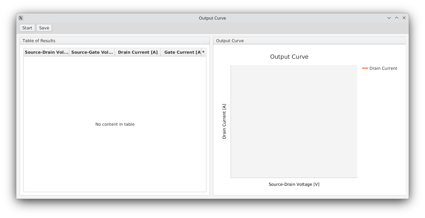
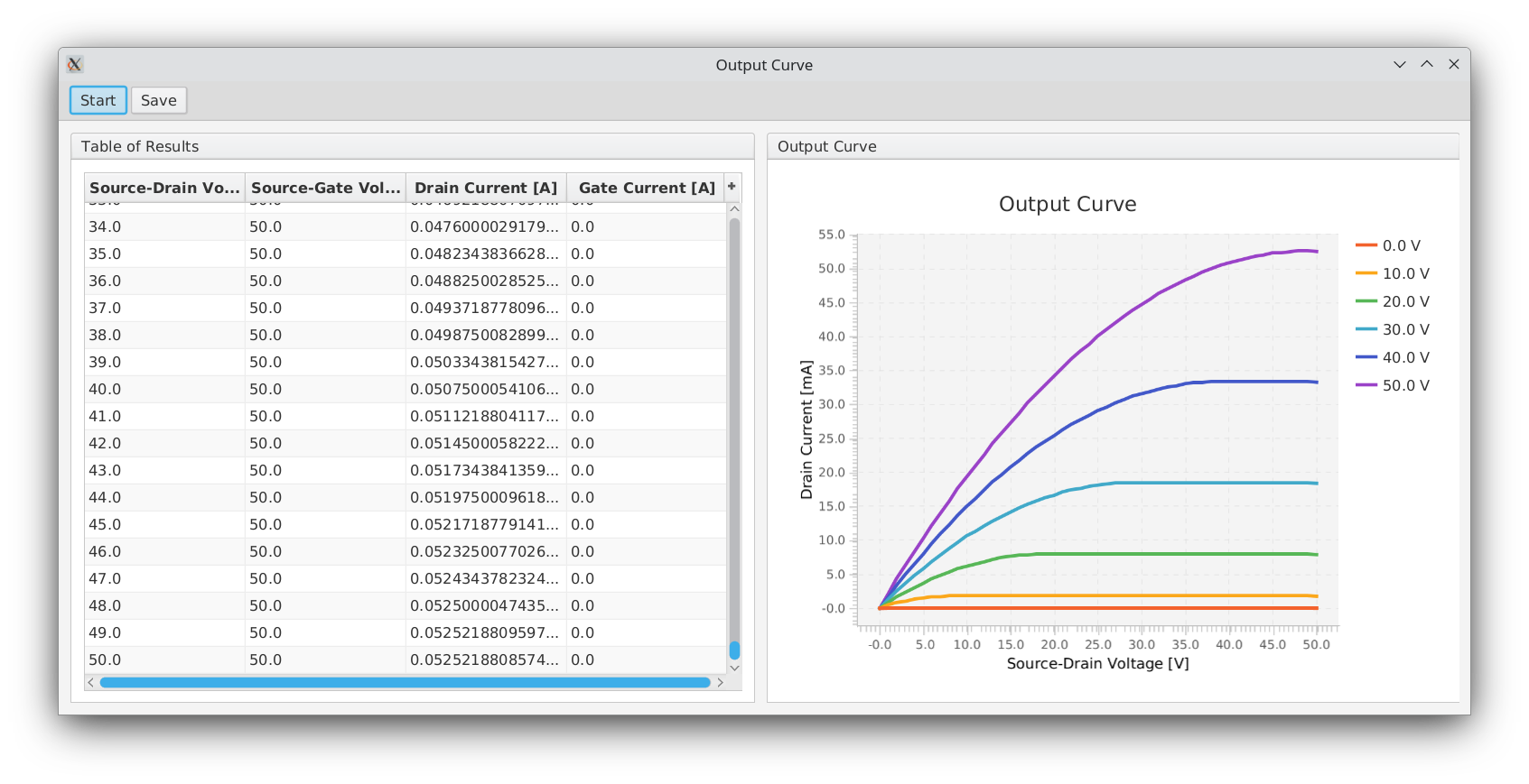
Figure 3: The result of running the example program (outputCurve(...)), before pressing start (top), and after completing (bottom).

References

- [1] IEEE Standard Digital Interface for Programmable Instrumentation. Standard, Institute of Electrical and Electronics Engineers, Nov 1978.
- [2] IEEE Standard Codes, Formats, Protocols, and Common Commands for Use With IEEE Std 488.1-1987, IEEE Standard Digital Interface for Programmable Instrumentation. Standard, Institute of Electrical and Electronics Engineers, Nov 1992.
- [3] Standard commands for programmable instruments. Standard, SCPI Consortium, IVI Foundation, Nov 1999.
- [4] The Authoritative Dictionary of IEEE Standards Terms, Seventh Edition. IEEE Std 100-2000, page 574, 2000.
- [5] PyMeasure Team. PyMeasure. GitHub Repository https://github.com/pymeasure/pymeasure, 2022.
- [6] Qusay H Mahmoud. Practice and experience with java in education. Science of Computer Programming, 53(1):1–2, 2004.
- [7] FAIR Facility for Anti-Proton and Ion Research. ChartFX. GitHub Repository https://github.com/fair-acc/chart-fx, 2022.
- [8] Youcheng Zhang, Amita Ummadisingu, Ravichandran Shivanna, Dionisius Hardjo Lukito Tjhe, Hio-Ieng Un, Mingfei Xiao, Richard H Friend, Satyaprasad P Senanayak, and Henning Sirringhaus. Direct observation of contact reaction induced ion migration and its effect on non-ideal charge transport in lead triiodide perovskite field-effect transistors. Small, page 2302494, 2023.
- [9] William A Wood, Ian E Jacobs, Leszek J Spalek, Yuxuan Huang, Chen Chen, Xinglong Ren, and Henning Sirringhaus. Revealing contributions to conduction from transport within ordered and disordered regions in highly doped conjugated polymers through analysis of temperature-dependent hall measurements. Physical Review Materials, 7(3):034603, 2023.
- [10] Dionisius Hardjo Lukito Tjhe, Xinglong Ren, Ian Jacobs, Tarig Mustafa, Thomas Marsh, Yuxuan Huang, Lu Zhang, William Wood, Ahmed Mansour, Gabriele d’Avino, et al. Thermoelectric transport signatures of carrier interactions in polymer electrochemical transistors. Bulletin of the American Physical Society, 2023.
- [11] Satyaprasad P Senanayak, Krishanu Dey, Ravichandran Shivanna, Weiwei Li, Dibyajyoti Ghosh, Youcheng Zhang, Bart Roose, Szymon J Zelewski, Zahra Andaji-Garmaroudi, William Wood, et al. Charge transport in mixed metal halide perovskite semiconductors. Nature Materials, 22(2):216–224, 2023.
- [12] Ian E. Jacobs, Gabriele D’Avino, Vincent Lemaur, Yue Lin, Yuxuan Huang, Chen Chen, Thomas F. Harrelson, William Wood, Leszek J. Spalek, Tarig Mustafa, Christopher A. O’Keefe, Xinglong Ren, Dimitrios Simatos, Dion Tjhe, Martin Statz, Joseph W. Strzalka, Jin-Kyun Lee, Iain McCulloch, Simone Fratini, David Beljonne, and Henning Sirringhaus. Structural and dynamic disorder, not ionic trapping, controls charge transport in highly doped conducting polymers. Journal of the American Chemical Society, page jacs.1c10651, 2 2022.
- [13] Yuxuan Huang, Dionisius Hardjo Lukito Tjhe, Ian E Jacobs, Xuechen Jiao, Qiao He, Martin Statz, Xinglong Ren, Xinyi Huang, Iain McCulloch, Martin Heeney, et al. Design of experiment optimization of aligned polymer thermoelectrics doped by ion-exchange. Applied Physics Letters, 119(11), 2021.
- [14] Martin Statz, Severin Schneider, Felix J Berger, Lianglun Lai, William A Wood, Mojtaba Abdi-Jalebi, Simone Leingang, Hans-Jorg Himmel, Jana Zaumseil, and Henning Sirringhaus. Charge and thermoelectric transport in polymer-sorted semiconducting single-walled carbon nanotube networks. ACS nano, 14(11):15552–15565, 2020.
- [15] Martin Statz, Severin Schneider, Felix Berger, Lianglun Lai, William Wood, Jana Zaumseil, and Henning Sirringhaus. Temperature-dependent thermoelectric transport in polymer-sorted semiconducting carbon nanotube networks with different diameter distributions. Bulletin of the American Physical Society, 65, 2020.