Business Metric-Aware Forecasting for Inventory Management

Abstract

Time-series forecasts play a critical role in business planning. However, forecasters typically optimize objectives that are agnostic to downstream business goals and thus can produce forecasts misaligned with business preferences. In this work, we demonstrate that optimization of conventional forecasting metrics can often lead to sub-optimal downstream business performance. Focusing on the inventory management setting, we derive an efficient procedure for computing and optimizing proxies of common downstream business metrics in an end-to-end differentiable manner. We explore a wide range of plausible cost trade-off scenarios, and empirically demonstrate that end-to-end optimization often outperforms optimization of standard business-agnostic forecasting metrics (by up to 45.7% for a simple scaling model, and up to 54.0% for an LSTM encoder-decoder model). Finally, we discuss how our findings could benefit other business contexts.

1 Introduction

Time-series forecasting is an essential component of decision-making and planning. In industries ranging from healthcare (Jones et al.,, 2009; Reich et al.,, 2019; Cheng et al.,, 2021), to finance (Thomas,, 2000; Elliott and Timmermann,, 2016), to energy (Ahmed et al.,, 2020; Donti and Kolter,, 2021), businesses leverage forecasts of future demand in order to adjust their behavior accordingly.

One common business problem reliant on time-series forecasts is inventory management (Chopra et al.,, 2007; Syntetos et al.,, 2009). Here, businesses must decide how much inventory to order on a recurring basis, balancing considerations such as customer satisfaction, costs of holding surplus inventory (holding cost), opportunity costs of out-of-stock items (stockout cost), and keeping the supply chain running smoothly. For example, grocery stores track their inventory, anticipating demand and placing orders such that when customers demand e.g. toilet paper, they have enough stock to avoid lost sales and keep customers happy, while not having too much stock such that stale items are taking valuable shelf or warehouse space.

Since forecasts are used to decide how much inventory to order, the quality of forecasts can greatly influence downstream measures of business performance. Typically, forecasters optimize and evaluate generic metrics agnostic to the downstream application, such as mean squared error (MSE) or mean absolute percentage error (MAPE). Assuming that these upstream forecasts are accurate, downstream decisions are subsequently treated as a separate step (Figure 1).

However, these generic metrics can be misaligned with downstream business performance. For example, the business costs of over-forecasting and under-forecasting are often imbalanced (e.g. opportunity cost of lost sales could outweigh cost of holding extra inventory). Additionally, conventional forecasting metrics typically aim for a mean, median, or quantile of the distribution, without regard to the magnitude of fluctuations in predictions. Fluctuations in predictions can translate into fluctuations in orders, and as orders are passed upstream through the supply chain, uncertainties in forecasts can compound to create the bullwhip effect, an unstable and wildly oscillating demand (Lee et al.,, 1997; Wang and Disney,, 2016).

One reason for the widespread use of generic accuracy metrics such as MSE and MAPE is that downstream business metrics may be difficult to quantify or attribute to specific parts of the supply chain. Customer satisfaction, for example, might have a convoluted data generating process that is difficult to optimize directly. However, as we show, optimization of generic metrics does not necessarily translate into improvements on downstream performance indicators.

In this work, we propose a novel method for business metric-aware forecasting for inventory management systems. Our contributions include:

1. Demonstrating that optimizing conventional metrics often translates into sub-optimal downstream performance.

2. Deriving an efficient end-to-end differentiable procedure for optimizing forecasts for downstream inventory performance, compatible with any differentiable forecaster.

3. Noting that downstream metrics are often at odds with one another, and proposing alternative combined objectives which trade off these metrics in different ways.

4. Empirically demonstrating the benefit of business metric-aware forecasting in univariate and multivariate datasets, under a variety of plausible downstream scenarios.

5. Since time series datasets measuring demand are popular in the forecasting community, we release code for others to evaluate the downstream utility of their forecasts.

Figure 1: Typical separated estimation and optimization approach, where the learned forecaster (blue) is agnostic to business decision-making (green). Solid lines represent direct optimization. This work solidifies the dotted green lines.

2 Related Work

Forecasting + Inventory Optimization

Inventory management involves estimating future demand (forecasting) and deciding how many orders to place to minimize costs and meet customer needs (inventory optimization). Some works simply forecast the mean demand and treat it as the inventory optimization solution (Yu et al.,, 2013; Ali and Yaman,, 2013). However, this approach fails to account for imbalanced costs of over- and under-forecasting. Thus, in practice, it is common to take a separated estimation and optimization approach (Turken et al.,, 2012; Oroojlooyjadid et al.,, 2020), which involves first (1) forecasting demand and then (2) plugging the estimates into inventory optimization (Figure 1). However, in this approach, errors in forecasting and inventory optimization can compound.

One widely studied inventory model is the newsvendor problem, which involves determining the optimal order quantity for perishable or seasonal products to balance holding cost and stockout cost. In this setup, the optimal solution to the inventory optimization problem is a particular quantile of the demand distribution (Petruzzi and Dada,, 1999). Thus, some works forecast various quantiles of the demand distribution (Böse et al.,, 2017; Bertsimas and Thiele,, 2005; Taylor,, 2000). Others use feed-forward neural networks, kernel regression, and linear models to directly optimize these two costs (Ban and Rudin,, 2019; Oroojlooyjadid et al.,, 2017). We also optimize downstream inventory metrics directly, but allow more general cost objectives to be computed over the inventory system variables through use of differentiable simulation, making our approach applicable beyond newsvendor.

Demand Forecasting

Demand forecasting is of interest in several businesses, including retail (Fildes et al.,, 2022), power grids (Ghalehkhondabi et al.,, 2017; Suganthi and Samuel,, 2012), emergency care (Jones et al.,, 2009), and municipal water (Donkor et al.,, 2014). Techniques for forecasting include both classical statistical and modern deep learning approaches. Traditional time-series forecasting methods include autoregressive (AR) models (Box et al.,, 2015; Makridakis and Hibon,, 1997), exponential smoothing (Gardner Jr,, 1985; Winters,, 1960), and the Theta model (Assimakopoulos and Nikolopoulos,, 2000; Hyndman and Billah,, 2003). Deep learning architectures for time-series forecasting include convolutional neural networks (Bai et al.,, 2018; Oord et al.,, 2016), recurrent neural networks (Hochreiter and Schmidhuber,, 1997; Salinas et al.,, 2020; Rangapuram et al.,, 2018), and attention-based methods (Fan et al.,, 2019; Li et al.,, 2019; Lim et al.,, 2021), among others (Oreshkin et al.,, 2019; Challu et al.,, 2022). However, these works all optimize business-agnostic metrics.

Inventory Optimization

Given demand forecasts, the decision of how many orders to place could be treated as a constrained optimization problem (Dai et al.,, 2021), a supervised deep learning problem (Qi et al.,, 2023), or a reinforcement learning problem (Oroojlooyjadid et al.,, 2017). There are also several common practices for placing orders (Eilon and Elmaleh,, 1968). For example, the (T, S) policy places orders every T days, and orders up to an inventory level S. Petropoulos et al., (2019) explored the inventory performance of several traditional forecasting models when a fixed periodic order-up-to (T, S) policy is used, finding that methods based on combinations had superior inventory performance. We use the same order-up-to policy in this work, but instead of taking a separated estimation and optimization approach, we use differentiable simulation to optimize downstream business performance end-to-end.

Forecasting Competitions

Forecasting competitions such as the M-Competitions (Makridakis and Hibon, 2000a, ; Makridakis et al.,, 2020, 2022) and the Favorita Competition (Favorita,, 2017) have become popular benchmarks for development of modern time-series forecasting methods. While a substantial portion of this data is industry time-series, evaluation of model performance is largely conducted using generic error metrics which ignore downstream business performance. For example, the M3 competition measured performance using versions of symmetric mean/ median absolute percentage error (sMAPE) and median relative absolute error. Submissions to the Favorita competition were evaluated using the normalized weighted root mean squared logarithmic error. By releasing inventory performance code, would like to further challenge researchers to make high-utility predictions on this data.

Inventory Performance Metrics

Across several inventory optimization applications, ranging from auto parts suppliers (Qi et al.,, 2023), to online fashion retailers (Ferreira et al.,, 2016), to drug inventories (Dhond et al.,, 2000), the common objectives of interest are typically a function of stockout cost and holding cost. These costs may be computed across various lead times, different parts of the supply chain, or simply based on historical data. High variance of orders has also been identified as an undesirable phenomenon due to the bullwhip effect in supply chains (Lee et al.,, 1997; Petropoulos et al.,, 2019), in which fluctuations in downstream demand can cause exaggerated order swings upstream in the supply chain that result in customer-upsetting stockouts and wasteful excesses.

3 Inventory Management

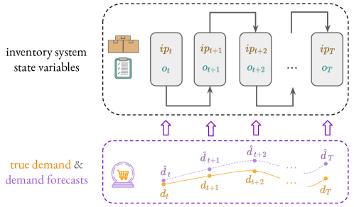
Figure 2: Inventory management systems keep track of state variables such as the current inventory position $ip$ and orders placed $o$. Inventory position is decreased based on observed demand $d$, and replenished by orders $o$ which are placed based on demand forecasts $\widehat{d}$ and the current $ip$.

This section formalizes the quantities used and tracked in an inventory management system (Figure 2), and defines business-aware and business-agnostic metrics of interest.

3.1 Formulation

For each time-series, we apply a rolling simulation approach in order to simulate an inventory system as it steps through each time point. Consider a time-series of the true demand $d_{t}$ at every time point $t=1,2,...,T$. At each $t$, orders $o_{t}$ are placed with the expectation that they will take lead-time $L$ to come in. Using the order-up-to policy for inventory replenishment (Gilbert,, 2005; Petropoulos et al.,, 2019), orders are given by:

$$o_{t}=\widehat{D}_{t}^{L}+ss_{t}-ip_{t}$$ (1)

where $\widehat{D}_{t}^{L}$ is the forecasted lead-time demand over the next $L$ timesteps, $ss_{t}$ is safety stock that adds a buffer to ensure that the orders placed cover the demand, and $ip_{t}$ is the inventory position. The true lead-time demand $D_{t}^{L}$ and the forecasted lead-time demand $\widehat{D}_{t}^{L}$ are given by:

$$D_{t}^{L}=\sum_{k=1}^{L}d_{t+k},\hskip 30.00005pt\widehat{D}_{t}^{L}=\sum_{k=1}^{L}\widehat{d}_{t,t+k}$$ (2)

where $\widehat{d}_{t,t+k}$ is the forecast of demand for time $t+k$ given data up to time $t$. Safety stock is computed as follows:

$$ss_{t}=\Phi^{-1}(\alpha_{s})\sigma_{e},$$ (3)

where $\sigma_{e}$ is the standard deviation of the forecast errors, and $\Phi^{-1}(\alpha_{s})$ is the inverse CDF of the normal distribution evaluated at some target service level $\alpha_{s}$. Assuming normally-distributed errors, with $\alpha_{s}$ probability, the safety stock plus lead time demand forecast should cover the actual demand.

Inventory position $ip_{t}$ is obtained by taking the previous inventory position, adding the orders $o_{t-1}$ from the previous timestep, and subtracting the current demand $d_{t}$:

$$ip_{t}=ip_{t-1}+o_{t-1}-d_{t}.$$ (4)

We assume $ip_{0}=0$ and $o_{0}=0$. Since orders take lead time $L$ to arrive, the inventory position can be decomposed into a sum of (a) how much inventory is actually on hand, termed net inventory level $i_{t}$, and (b) how much inventory is on the way, termed work-in-progress level $w_{t}$:

• Inventory position: $ip_{t}=i_{t}+w_{t}$

• Net inventory: $i_{t}=i_{t-1}+o_{t-L}-d_{t}$

• Work-in-progress: $w_{t}=w_{t-1}+o_{t-1}-o_{t-L}$

In summary, at each time $t$, orders $o_{t}$ are placed based on forecasted lead-time demand $\widehat{D}_{t}^{L}$ and the current inventory position $ip_{t}$. The orders and current demand then adjust the inventory position $ip_{t+1}$, and this process repeats for the entire length $T$ of the time-series.

3.2 Evaluation Metrics

We evaluate and optimize both downstream business performance and conventional generic forecasting metrics.

3.2.1 Downstream Inventory Performance

One straightforward way to balance excess inventory, lost sales, and stability of orders is to frame everything in terms of cost. Thus we introduce a total cost metric, measured in units of money. We also introduce a unitless metric, relative root-mean-square, which compares the performance versus a simple baseline.

Total cost (TC) is defined as a combination of the cost of holding excess inventory (holding cost $C_{h}$), the opportunity cost of running out of stock (stockout cost $C_{s}$), and the cost of fluctuations in the supply chain (order variance cost $C_{v}$):

$$C_{h} =c_{h}\cdot\mathbb{E}_{t}[\text{max}(0,i_{t})]$$

$$C_{s} =c_{s}\cdot\mathbb{E}_{t}[\text{max}(0,-i_{t})]$$

$$C_{v} =c_{v}\cdot\text{Var}_{t}(o_{t})$$

$$TC =C_{h}+C_{s}+C_{v},$$

where expectations are taken over all time points $t$, and $c_{h},c_{s},c_{v}\geq 0$ are constants. Specifically, $c_{h}$ is the unit holding cost, $c_{s}$ is the unit stockout cost, and $c_{v}$ is the unit order variance cost. If this information is available in a given problem setting, one can directly plug it in. Otherwise, practitioners can choose how to balance these different factors based on their domain expertise. For example, one might have the intuition that sales lost are more expensive per unit than the cost of holding an extra unit of inventory. If the different components of a supply chain are well-integrated so that the compounded uncertainty is not a major concern, the unit order variance cost may not need to be large.

For settings in which the cost tradeoffs may be unknown, we introduce the relative root-mean-square (RRMS) metric:

$$RRMS =\sqrt{\text{rel}(C_{h})^{2}+\text{rel}(C_{s})^{2}+\text{rel}(C_{v})^{2}},$$

where relative performance to a naive baseline is defined as

$$\text{rel}(x) =\sigma\left(\frac{x-x_{naive}}{x_{naive}}\right),$$

where $\sigma$ is a sigmoid function. The naive baseline we use in our experiments is a model which simply outputs the previous observation from one period ago. Note that the $rel(x)$ is a unitless quantity, as the unit costs cancel out in the numerator and denominator.

3.2.2 Generic Forecasting Metrics

We also evaluate and optimize generic forecasting metrics to understand the extent to which they might indirectly optimize for downstream performance. Mean squared error (MSE) is given by averaging the squared error over time points 1 to $T$ and forecasting horizons 1 to $H$:

MSE $$=\frac{1}{TH}\sum_{t=1}^{T}\sum_{k=1}^{H}\left(d_{t+k}-\widehat{d}_{t,t+k}\right)^{2}.$$

Symmetric mean absolute percentage error (sMAPE) is:

$$\text{sMAPE}=\frac{1}{TH}\sum_{t=1}^{T}\sum_{k=1}^{H}\frac{|d_{t+k}-\widehat{d}_{t,t+k}|}{|d_{t+k}|+|\widehat{d}_{t,t+k}|}\times 2.$$

4 Methods

Several challenges arise in optimization of downstream business metrics. Here, we describe how persistent state variables can be computed differentiably, how to optimize for objectives that are computed over the entire time-series of these state variables rather than point-wise, how to provide additional supervision for univariate time series, and how to simulate how models would be updated over time as new data points are observed. Additionally, we describe the models, datasets, and experiment setup.

4.1 Differentiable Computation of Metrics

For typical forecasting metrics (e.g. MSE, sMAPE, etc.), differentiable computation is relatively straightforward. These metrics can usually be decomposed such that at each time point, some differentiable quantity (e.g. squared difference of prediction and actual value) is computed, and an average over time points is taken. Computing inventory performance (e.g. total cost, RRMS), however, is less straightforward as there are persistent inventory state variables (e.g. net inventory level, orders) that must be tracked over time. Although inventory performance is not in general a differentiable quantity, we derive a series of computations which can simulate the inventory management system and order-up-to policy described by (1)–(4) in a differentiable manner. Composing this system with the outputs of a differentiable forecaster, we create an end-to-end differentiable system.

Naively, one could iterate over each time point, and apply the recursive inventory state update equations (1)–(4). However, for long time-series this would be computationally infeasible, due to the instability of backpropagation through a long chain of dependent states (Pascanu et al.,, 2013). Instead, assuming all quantities at time $t<0$ are 0, we show by expanding out the recursion (derivations in Appendix) that the orders at any time $t$ can be written in closed form:

$$o_{t}=(\widehat{D}_{t}^{L}-\widehat{D}_{t-1}^{L})+\Phi^{-1}(\alpha_{s})\cdot(\sigma_{e,t}-\sigma_{e,t-1})+d_{t}$$ (5)

and the net inventory at time $t$ can be written as:

$$i_{t} =\widehat{D}_{t-L}^{L}+\Phi^{-1}(\alpha_{s})\cdot\sigma_{e,t-L}-\sum_{a=t-L+1}^{t}d_{a}.$$ (6)

These closed form equations are much more efficient to implement in terms of tensor operations than the original recursive equations, and they allow us to simultaneously compute the net inventory levels and orders at all times given a tensor of demand forecasts at all times (detailed walkthrough in the Appendix).

Given the inventory state variables $o_{t}$ and $i_{t}$ for all $t$, it is now feasible to compute metrics on top of these variables. Holding and stockout costs can be computed by applying a ReLU activation over $i_{t}$ and $-i_{t}$, and computing the average over timepoints. Variance of orders can be computed by averaging the squared difference between orders and the average number of orders. Finally, combinations or simple differentiable functions of these quantities can straightforwardly computed to yield both total cost (TC) and the relative root-mean-square metric (RRMS) (details in Appendix).

4.2 Double-Rollout Supervision

Another challenge of optimizing downstream inventory performance is that some aspects must be computed holistically across multiple time points (e.g. order variance). For univariate time-series where a local model is trained on only one time-series, this is especially challenging due to limited supervision. To provide more supervision, we use a custom training method where at each time point, an inventory system simulation is rolled out over the next $H$ time points, where forecasting horizon $H>L$. By simulating the inventory system several times using different starting points in the univariate time-series, one can obtain several evaluations of TC and RRMS to serve as supervision from just one time-series (see Appendix for diagram). For multivariate time-series, instead of forecasting for a horizon $H>L$ and then unrolling lead-time demands across that horizon, only forecasts of the requisite lead time $L$ are made since the other time-series can provide supervision, and double-rollouts are more computationally expensive.

4.3 Roll-Forward Evaluation

In real-world settings, as new data are collected, forecasting models are updated and decisions are made accordingly. To simulate this process, we employ a training procedure which rolls forward in time. For each time point from $t=1$ to $t=T$, the model is trained with data up to $t$ using double-rollout supervision for univariate time-series, and single-rollout supervision for multivariate time-series. Then, the model forecasts the next $L$ timesteps after $t$, i.e. $\widehat{d}_{t,t+k}$ for all $k\in\{1,2,...,L\}$. After all $T$ timesteps have been trained on and forecasted from, giving a $N\times T\times L$ tensor, inventory performance is computed over the $T$ timepoints. For each dataset we designate training, validation, and test time ranges, where validation data is used for hyperparameter tuning, and test data is used for reporting final performance.

4.4 Models

We explore two differentiable models for forecasting: (1) a seasonal scaling model, and (2) an LSTM encoder-decoder model. For univariate time-series, one local model is trained per time-series, and for multivariate time-series, one global model is trained across all time-series. Hyperparameter and model training details are in the Appendix.

Naive Seasonal Scaling Model

This model has one learnable parameter $\beta\in\mathbb{R}$, the amount to scale observations from one period $P$ ago. That is, $\widehat{d}_{t,\text{seasonal scaler}}=\beta\cdot d_{t-P}.$ This model is valuable from an interpretability perspective, as $\beta>1$ could indicate a preference towards over-forecasting versus the previous period of data, and $\beta<1$ could indicate a preference towards under-forecasting.

LSTM Encoder-Decoder

This model has an LSTM encoder which sequentially encodes a window of inputs, and an LSTM decoder which sequentially decodes to yield predictions across a forecasting horizon. For multivariate time-series, the covariates are embedded before being fed into the encoder, and a linear layer is used on top of the outputs of the decoder to yield the forecasts. See the Appendix for a diagram of the model architecture.

4.5 Data

4.5.1 M3 Monthly Industry Subset (Univariate)

The monthly industry subset of the M3 competition data Makridakis and Hibon, 2000b consists of 334 univariate time-series with up to 144 time points, where time points occur on a monthly basis. As described by Petropoulos et al., (2019), this subset can serve as a proxy for demand on a monthly basis. These time-series are not aligned by start date, have varying lengths, and are not directly related to each other. Hence, each time-series in this dataset is treated separately as a univariate time-series for modeling purposes.

4.5.2 Favorita Grocery Sales (Multivariate)

The Corporación Favorita Grocery Sales Forecasting dataset Favorita, (2017) consists of sales data across several stores and products. The dataset includes covariates such as oil prices, location, day of week, month, and holidays. We use a similar preprocessing pipeline as in Lim et al., (2021) to yield 90,193 distinct time-series with up to 396 time points, where time points occur on a daily basis from 2015 to 2016. As grocery replenishment often occurs on a daily basis, the inventory system is updated daily. These time-series are aligned to start at the same time in the real world, missing values are imputed with zeros, and the time-series are likely correlated with each other since they are all associated with sales in Corporación Favorita. Thus, this dataset is treated as a multivariate time-series dataset, and one global model is learned.

4.6 Experiment Setup

The models are optimized using the mean squared error (MSE), relative root mean square (RRMS), and total cost (TC) objectives across several settings of unit costs.

For M3, a separate local model is trained with double-rollout supervision and roll-forward evaluation for each of the 334 univariate time-series. Since each time point corresponds to one month, a periodicity of $P=12$ is used for seasonal models. An encoding window of 24 months is used as input to the model, allowing the model to learn use the previous two periods of history for its predictions. Predictions are made for a forecasting horizon of 12 months, so that the double-rollout can compute inventory performance over multiple time points. A lead time of $L=6$ months is used. Out of 144 months, forecasting models are initially trained with 72 months, then validated until 108 months, and then tested until 144 months. Since the safety stock discouraged forecasting errors, whereas a high or low unit holding cost could encourage over- or under-forecasting, we choose to have $\alpha_{s}=0.5$, so $ss_{t}=0$ for all $t$, to avoid unstable interactions between unit costs and safety stocks. For the TC objective, models are trained on every combination of unit holding costs $c_{h}\in\{1,2,10\}$, unit stockout costs $c_{s}\in\{1,2,10\}$, and unit order variance costs $c_{v}\in\{1\mathrm{e}{-6},1\mathrm{e}{-5}\}$ (chosen based on the order of magnitude of demand).

For Favorita, one global model is trained with single-rollout supervision and roll-forward evaluation for all 90,193 multivariate time-series. A global model is used because all time-series are aligned and correlated with one another, and training a separate model for each series would be computationally expensive. Each time point corresponds to one day, so a periodicity of $P=7$ is used. An encoding window of 90 days is input to the model, which forecasts the next 30 days. A lead time of $L=7$ days is used. Out of 396 days, the training cutoff is at day 334, the validation cutoff is day 364, and the remainder is used for testing. Again, we set $\alpha_{s}=0.5$. For the TC objective, due to more expensive training, a subset of $N=10,000$ samples are extracted to test all combinations of unit holding costs $c_{h}\in\{1,2,10\}$, unit stockout costs $c_{s}\in\{1,2,10\}$, and unit order variance costs $c_{v}\in\{1\mathrm{e}{-3},1\mathrm{e}{-2}\}$.

5 Results

Unit Cost-Agnostic Performance

Tables 1 and 2 characterize the performance of several forecasters trained on the full M3 and Favorita datasets when evaluated on typical forecasting metrics, MSE and sMAPE, and an inventory performance metric, RRMS. All of the models in these tables are trained and evaluated on objectives that are agnostic to unit costs $c_{h},c_{s},$ and $c_{v}$.

In both M3 and Favorita, the Seasonal Scaler and LSTM models trained with MSE objective perform competitively with classical models on MSE and sMAPE, either performing better than or within the range of performance spanned by the ARIMA, Exponential Smoothing, and Theta models. In the M3 dataset, the model with best RRMS is the seasonal scaler trained on RRMS—abbreviated as Seasonal Scaler (RRMS). However, it achieves worse MSE (22.10$\times 10^{5}$) than the Seasonal Scaler (MSE), LSTM (MSE), Exponential Smoothing, and Theta models (MSEs ranging 13.82$\times 10^{5}$ to 20.89$\times 10^{5}$). In the Favorita dataset, the Seasonal Scaler (MSE) and the Seasonal Scaler (RRMS) outperform all other models on RRMS, despite having worse MSE (1.23$\times 10^{2}$ and 1.25$\times 10^{2}$) than the LSTM (MSE), ARIMA, and Theta models (0.88$\times 10^{2}$ to 1.12$\times 10^{2}$). On the M3 dataset, the LSTM (MSE) achieves the best MSE (13.82$\times 10^{5}$), yet has the second to worst RRMS (1.23). On Favorita, the LSTM (MSE) objective again achieves the best MSE (0.88$\times 10^{2}$), yet has the worst RRMS (1.17). Overall, performance on typical forecasting metrics (MSE and sMAPE) appears misaligned with relative inventory performance (RRMS), and optimizing for one does not inherently seem to optimize for the other.

Table 1: M3 test performance of models that are agnostic to unit costs. Note that the best-performing models on MSE are misaligned with the best-performing models on RRMS.

Model (Objective)	MSE	sMAPE	RRMS
	($\times 10^{-5}$)
Seasonal Scaler (MSE)	20.89	0.27	1.27
Seasonal Scaler (RRMS)	22.10	0.28	0.74
LSTM (MSE)	13.82	0.24	1.23
LSTM (RRMS)	226.49	1.25	1.02
ARIMA	25.78	0.34	1.12
Exponential Smoothing	15.21	0.24	1.12
Theta	14.00	0.22	1.09

Table 2: Favorita test performance of models that are agnostic to unit costs. Note the best-performing models on MSE are misaligned with the best-performing models on RRMS.

Model (Objective)	MSE	sMAPE	RRMS
	($\times 10^{-2}$)
Seasonal Scaler (MSE)	1.23	1.51	0.85
Seasonal Scaler (RRMS)	1.25	1.73	0.94
LSTM (MSE)	0.88	1.77	1.17
LSTM (RRMS)	3.42	2.84	1.10
ARIMA	1.12	1.76	1.06
Exponential Smoothing	1.36	1.80	1.10
Theta	1.08	1.81	1.09

Table 3: M3 test total cost across several unit cost settings $(c_{h},c_{s},c_{v})$.

Model (Objective)	(1, 1, 1e-05)	(1, 1, 1e-06)	(1, 10, 1e-05)	(1, 10, 1e-06)	(10, 1, 1e-05)	(10, 1, 1e-06)
LSTM (MSE)	5,826	5,435	39,519	39,128	20,660	20,269
LSTM (RRMS)	17,188	17,102	170,738	170,652	17,474	17,388
LSTM (TC)	6,390	5,997	36,086	35,805	10,146	10,400
Seasonal Scaler (MSE)	5,680	5,372	43,791	43,483	15,610	15,302
Seasonal Scaler (RRMS)	5,771	5,476	45,216	44,920	15,314	15,018
Seasonal Scaler (TC)	5,185	4,884	35,268	34,918	12,178	11,996

Table 4: Favorita test total cost across several unit cost settings $(c_{h},c_{s},c_{v})$.

Model (Objective)	(1, 1, 1e-02)	(1, 1, 1e-03)	(1, 10, 1e-02)	(1, 10, 1e-03)	(10, 1, 1e-02)	(10, 1, 1e-03)
LSTM (MSE)	26.94	20.30	158.65	152.01	71.25	64.61
LSTM (RRMS)	94.51	72.08	162.55	140.12	652.76	630.33
LSTM (TC)	24.69	18.39	115.72	116.40	35.96	29.72
Seasonal Scaler (MSE)	24.52	21.22	200.51	197.22	36.25	32.96
Seasonal Scaler (RRMS)	23.40	18.69	158.51	153.80	51.84	47.13
Seasonal Scaler (TC)	23.52	18.51	118.48	107.03	32.68	30.18

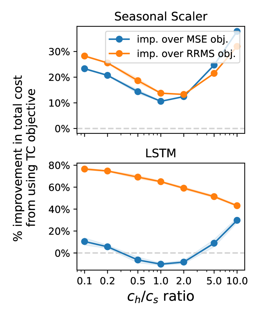
(a) M3

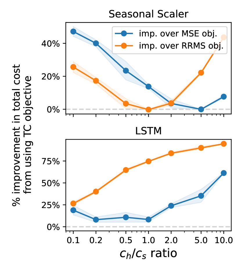
(b) Favorita

Figure 3: Average relative percentage improvement in test total cost from using the TC objective over the MSE objective and RRMS objective across various $c_{h}/c_{s}$ ratios. 95% CI are computed across different $c_{v}$ values.

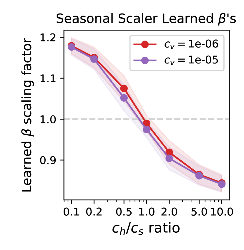
(a) M3

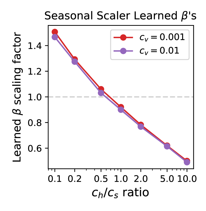
(b) Favorita

Figure 4: Learned scaling factors for the naive seasonal scaler on the M3 (left) and Favorita (right) datasets, across several unit cost tradeoffs. Dotted line corresponds to $\beta=1$.

Performance Across Several Unit Cost Tradeoffs

Tables 3 and 4 contain the test total cost across various unit cost settings. While Seasonal Scaler observes some benefit from training using the RRMS objective, it appears to cause unstable performance for the LSTM. On the other hand, using the TC objective almost always improves the total cost of the Seasonal Scaler and LSTM models, except for the LSTM on the M3 dataset, where a more consistent benefit is observed for imbalanced $c_{h}$ and $c_{s}$ (Figure 3 and Appendix Figure 11). The greater the imbalance in $c_{h}$ and $c_{s}$, the greater the improvement from using TC objective. For example, on Favorita, the Seasonal Scaler trained on TC achieves a 45.7% improvement over that trained by MSE when $(c_{h},c_{s},c_{v})=(1,10,10^{-3})$, and the LSTM encoder-decoder trained on TC achieves a 54.0% improvement over that trained by MSE when $(c_{h},c_{s},c_{v})=(10,1,10^{-3})$.

Leveraging the interpretability of the Seasonal Scaler model, we graph the relationship between the learned $\beta$s and the tradeoffs between $c_{h}$ and $c_{s}$ (Figure 4). In both M3 and Favorita, with larger $c_{h}/c_{s}$ ratios and increasing $c_{v}$, the learned $\beta$ scaling factor decreases.

Another benefit of end-to-end optimization of forecasts is interpretability that the forecasts themselves provide. Appendix Figure 10 plots the forecasted and true lead demands, averaged over all series in each dataset, for various cost objectives. When trained on MSE, the LSTM model tends to slightly over-forecast the true demand in aggregate, whereas the Seasonal Scaler model appears to match or slightly under-forecast. When trained on the TC objective, both models tend to under-forecast when the $c_{h}/c_{s}$ ratio is high, and over-forecast when the ratio is low. The LSTM predictions on M3 are smoother than that of the Seasonal Scaler, perhaps because the LSTM is more flexible and able to reduce the variance of its predictions in order to help reduce order variance, whereas the Seasonal Scaler can only scale the previous period by some constant (but note that due to roll-forward evaluation, where the model is updated each time point, this constant can change over time). The LSTM predictions on Favorita are more variable, perhaps due to the small order variance penalty.

6 Discussion

We demonstrate the limitations of using standard forecasting metrics that are agnostic to downstream business metrics, and propose a method for augmenting models with business metric-aware objectives. Common forecasting metrics such as MSE and sMAPE can be misaligned with downstream inventory performance, and optimizing for such metrics does not inherently optimize for inventory performance metrics (Tables 1 and 2). We derive a differentiable procedure for computing inventory performance, and demonstrate that especially when costs are imbalanced, utilizing a business metric-aware total cost objective often significantly improves downstream costs (Tables 3 and 4, Figures 3 and 11).

When deployed in a roll-forward evaluation framework, we observe that the Seasonal Scaler can be surprisingly effective (Table 1 and 2) in some cases despite only having one learned parameter. One possible explanation is that the learned constant can vary over time and adapt to new data each timestep as it is observed. In contrast to standard evaluation in which one assumes that the model is learned on data from a fixed time period and evaluated on a fixed test time period, this form of evaluation could be more realistic for the inventory management setting, where forecasts are constantly updated to inform daily, weekly, or monthly decisions. At the same time, the Seasonal Scaler must have an output proportional to the previous period which restricts the flexibility of this model class even if the proportion can change over time. The more flexible LSTM model performs best in MSE and in several of the cost tradeoff settings.

There are also some practical benefits of end-to-end optimization with business metric-aware objectives. When demand forecasting and inventory optimization are treated separately (as is typical), errors in each component are likely to compound. While some have proposed searching over conventional forecasting methods for models which happen to achieve better downstream inventory performance (Petropoulos et al.,, 2019), this is computationally expensive as several models must be trained, each of which have their own hyperparameters to be tuned. By directly optimizing end-to-end, this can save computation. Additionally, our methods for optimizing inventory performance are compatible with any differentiable forecaster.

More broadly, business metric-aware forecasting could be useful beyond inventory management, for other business problems that rely on forecasts. Through our case study in inventory, we have shown how to tackle some common challenges that might arise from attempting to simulate downstream decision-making processes and systems, including: (1) differentiable computation of persistent state variables, (2) optimization of objectives that must be computed over the entire time-series rather than point-wise, (3) providing additional supervision with limited time series, and (4) simulating how models would be updated over time as new data points are observed. Business decisions that rely on forecasts may inherently prefer error distributions that are biased in certain ways, and we encourage others to explore business metric-aware forecasting in their own business problems.

Limitations and Future Work

While TC outperforms MSE when costs are imbalanced, when costs balance each other out, the MSE objective can perform comparably or even slightly better than the TC objective (Figure 3(a), bottom). The TC objective, while differentiable, is more complex than MSE, and can be sensitive to hyperparameter tuning. Similarly, while RRMS is a convenient unitless objective, it can also be difficult to optimize. While in this work we decided to purely compare inventory vs. generic objectives, future work might explore pre-training with MSE and fine-tuning with TC or RRMS.

Finally, there are several possible avenues for further exploration. Future work could use the lens of business metric-aware forecasting to consider other differentiable model architectures, time series datasets, downstream objectives, and downstream business problems.

7 Acknowledgements

We gratefully acknowledge Kin Olivares, the Google Cloud AI Discovery, and Google Cloud Research teams for helpful conversations and feedback. This material is based upon work supported by the National Science Foundation Graduate Research Fellowship Program under Grant No. DGE1745016 and DGE2140739. Any opinions, findings, and conclusions or recommendations expressed in this material are those of the author(s) and do not necessarily reflect the views of the National Science Foundation.

Appendix A Differentiable Computation of Inventory Performance Metrics

In this appendix section we derive equations (5) and (4), and walk through differentiable computation of all inventory system variables.

Consider a model trained on $N$ univariate time-series, each with at most $T$ time points. Each time point, the model makes a lead-time forecast for the demand across a forecast horizon $L$. Thus, the model outputs a tensor $\widehat{d}=\mathbb{R}^{N\times T\times L}$, where an entry $\widehat{d}[i,t,l]$ corresponds to the forecasted demand in the $i$th series for time $t+l$ at time $t$.

A.1 Computing forecasted lead-time demand

The forecasted lead-time demand is $\widehat{D}_{t}^{L}=\sum_{l=1}^{L}\hat{d}[:,t,l]$, i.e. summation along the last axis of the $\widehat{d}$ tensor.

A.2 Computing orders

Here we derive equation (5). Alternating plugging in the inventory position equation (4) into the order-up-to policy equation (1) and recursively plugging in (1) to itself, we can expand the expression for orders into a closed form:

$$o_{t} =\widehat{D}_{t}^{L}+ss_{t}-ip_{t}$$

$$=\widehat{D}_{t}^{L}+ss_{t}-(ip_{t-1}+o_{t-1}-d_{t})$$

$$=\widehat{D}_{t}^{L}+ss_{t}-ip_{t-1}-(\widehat{D}_{t-1}^{L}+ss_{t-1}-ip_{t-1})+d_{t}$$

$$=(\widehat{D}_{t}^{L}-\widehat{D}_{t-1}^{L})+(ss_{t}-ss_{t-1})+d_{t}$$

$$=(\widehat{D}_{t}^{L}-\widehat{D}_{t-1}^{L})+\Phi^{-1}(\alpha_{s})\cdot(\sigma_{e,t}-\sigma_{e,t-1})+d_{t},$$

where the last step plugs in the safety stock definition (3). Using this equation we have derived, it is now possible to compute $o_{t}$ given just a tensor of demand forecasts $\widehat{d}$ and true demands $d$.

A.3 Computing net inventory

Here we derive the closed-form net inventory equation (6). Recursively plugging in the net inventory equation as well as the closed form expression for orders (5), we have:

$$i_{t} =i_{t-1}+o_{t-L}-d_{t}$$

$$=(i_{t-2}+o_{t-1-L}-d_{t-1})+o_{t-L}-d_{t}$$

$$=i_{0}+\sum_{j=0}^{t-L}o_{j}-\sum_{k=1}^{t}d_{k}$$

$$=i_{0}+\sum_{j=0}^{t-L}\left((\widehat{D}_{j}^{L}-\widehat{D}_{j-1}^{L})+(ss_{j}-ss_{j-1})+d_{j}\right)-\sum_{k=1}^{t}d_{k}$$

$$=i_{0}+\sum_{j=0}^{t-L}(\widehat{D}_{j}^{L}-\widehat{D}_{j-1}^{L}+ss_{j}-ss_{j-1})+d_{0}-\sum_{k=t-L+1}^{t}d_{k}$$

$$=i_{0}+\widehat{D}_{t-L}^{L}+\Phi^{-1}(\alpha_{s})\cdot\sigma_{e,t-L}+d_{0}-\sum_{k=t-L+1}^{t}d_{k},$$

assuming that all quantities at time $t=-1$ are equal to 0. Then, $i_{0}=i_{-1}+o_{-L}-d_{0}=-d_{0}$. Simplifying,

$$i_{t}=\widehat{D}_{t-L}^{L}+\Phi^{-1}(\alpha_{s})\cdot\sigma_{e,t-L}-\sum_{k=t-L+1}^{t}d_{k}.$$

Intuitively this makes sense, as the net inventory is determined by the lead time forecast from $L$ time steps prior, with additional safety stock estimated at the time, subtracting the interim demand leading up to the current time step. This closed form equation is much more efficient to implement in terms of tensor operations than the original recursive equation for inventory position. We have already described how to compute the first term, and the last term is simply the sum of true demands in a window of size $L$ leading up to time $t$. The 2nd term (safety stock) is computed by some constant $\Phi^{-1}(\alpha_{s})$ dependent on desired service level $\alpha_{s}$, multiplied by the standard deviation of forecast errors up until the previous time $\sigma_{e,t-1}$. Similar to the net inventory, we can also derive a closed-form expression for the inventory position: $ip_{t}=\widehat{D}_{t-1}^{L}+\Phi^{-1}(\alpha_{s})\cdot\sigma_{e,t-1}-d_{t}$, and the work in progress can simply be derived as $w_{t}=ip_{t}-i_{t}$.

A.4 Computing safety stock

The inverse CDF of the target service level $\Phi^{-1}(\alpha_{s})$ is a constant and straightforward to compute. The standard deviations of forecast errors $\sigma_{e,t}$ are more involved since forecasts are made at each time point for some horizon, but can be computed as follows:

• Create an $N\times T$ tensor $M$ where $M[:,t]=t$.

• Construct sliding windows of size $L$ along the time dimension. This will create a tensor $M^{\prime}$ with the same shape as $\widehat{d}$ ($N\times T\times L$), of the time of each entry.

• Repeat the tensor $T$ times in a new (fourth) dimension, thresholding to create a binary mask $M^{\prime\prime}$ for each $t\in\{1,2,...,T\}$ corresponding to whether that time has occurred. That is, $M^{\prime\prime}[i,t,l,t^{\prime}]=\mathbf{1}\left\{M^{\prime}[i,t,l,t^{\prime}]\leq t^{\prime}\right\}$.

• Compute per-element squared error $E$ of the $N\times T\times L$ predictions. Copy $T$ times to get $E^{\prime}$ ($N\times T\times L\times T$).

• Multiply the repeated error $E^{\prime}$ element-wise with the binary mask $M^{\prime\prime}$ (both should be $N\times T\times L\times T$). Sum along the second and third dimensions (of size $T$ and $L$), and divide by the sum of the binary mask along the second and third dimensions. This gives the average squared forecast errors for each time point, for each time-series. Take the square root to get the standard deviation.

A.5 Computing inventory performance metrics

There are three main aspects of inventory performance we examine:

1. Holding cost: $C_{h}=c_{h}\cdot\mathbb{E}[\text{max}(0,i_{t})]$

2. Stockout cost: $C_{s}=c_{s}\cdot\mathbb{E}[\text{max}(0,-i_{t})]$

3. Order variance cost: $C_{v}=c_{v}\cdot\text{Var}(o_{t})$

The holding cost can be computed by passing the computed inventory positions through a ReLU activation, and then taking the average across times and series. The variance of orders can be computed by taking the average orders for each series, subtracting them from the orders, squaring, and then taking the expectation.

The total cost (TC) and relative RMS (RRMS) objectives combine these three components in differentiable ways (either summation or subtracting and dividing by a constant, squaring, and summing).

Appendix B Double-Rollout Supervision

Here we describe the double-rollout supervision technique. Since some objectives must be computed holistically across multiple time points (e.g. order variance), a single series of points may only yield one inventory performance value. If one model is being trained per time series (as is the case in M3 univariate data), this provides very little supervision for the model. The double-rollout supervision technique addresses this problem by having the model predict a long forecasting horizon $H$, which is then treated as the series to compute inventory performance over (Figure 5, top). A sliding window of size $L$ is taken over the $H$ time points (Figure 5, bottom) in order to compute lead-time demands across the $H$ time points (Figure 6). Thus, we choose an $H>L$. If there are $t-W$ decoding points, then this gives $t-W$ series of length $\leq H$, which can provide $t-W$ measures of inventory performance to help supervise learning.

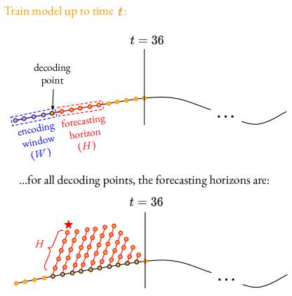
Figure 5: First step of the double-rollout training procedure. At each decoding point, the model forecasts a long forecasting horizon $H$.

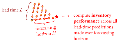
Figure 6: Second step of the double-rollout training procedure. For each forecasted horizon of $H$ time points, take a sliding window of size $L$ as the lead-time demand forecasts and compute inventory performance across the $H$ time points.

Appendix C Roll-Forward Evaluation

In real-world settings, models are updated over time as new data are collected. To better simulate the process of how forecasting models could feasibly be updated over time, we employ a training procedure which rolls forward in time.

At each time point $t=1,2,...,T$, the model is updated with the most recent data by taking additional gradient steps based on all data up to time $t$ (i.e. fine-tuning to the latest dataset each time). Given a model trained on the most recent demand data up time $t$, predictions are made for the next lead-time $L$ time steps (Figure 7), giving $\widehat{D}^{L}_{t}$ (Figure 8).

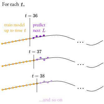
Figure 7: Each time $t$, the model is updated using all data available up until $t$, and forecasts the next $L$ time steps.

These predictions are used by the order-up-to policy (1) in order to determine how many orders to place at that time. This way, when inventory performance is computed across all $t$, the predictions are made using the most up-to-date models that could have been trained at each time point.

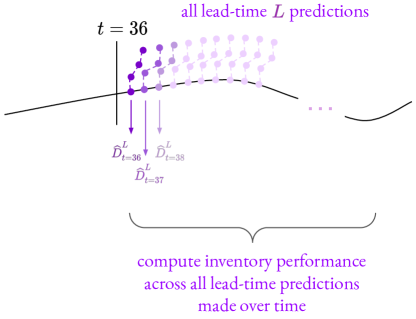
Figure 8: Predictions resulting from the roll-forward evaluation procedure after rolling across the whole series.

Appendix D Hyperparameter Selection

Ten iterations of random search with the MSE, TC, and RRMS objectives are used to choose hyperparameters for the M3 and Favorita datasets. For the Favorita dataset, a subset of 10,000 time series is used in order to tune hyperparameters more quickly. For the Naive Seasonal Scaler, the grid of hyperparameters considered is batchsize (100, 200, 300) and learning rate (0.01, 0.001, 0.0001). For the LSTM, the grid of hyperparameters considered is batchsize (100, 200, 300, 500), hidden size (32, 64, 128), and learning rate (0.01, 0.001, 0.0001, 0.00001). There is a small amount of subsequent manual tuning to try values beyond the grid if the best selected value was at the edge of the grid.

For the M3 dataset, a hidden size of 20 is used for both the encoder and decoder. For the Favorita dataset, a hidden size of 64 is used for both the encoder and decoder, and the embedding size is 10. Categorical variables are embedded such that each possible value is stored as a different learnable 10-dimensional vector, and numerical variables are passed through a linear layer with 10-dimensional output. The run_all.sh script in the included code supplement contains commands to run all of the experiments, with exact hyperparameter settings included.

Appendix E Training Details

On Favorita, LSTM encoder-decoder models are trained on machines with A100 GPUs, and require about 10GB of memory. On M3, LSTM encoder-decoder models are trained on machines with 32 CPUs, and since one model is trained for each series, model training is done in parallel, taking about 2GB of memory at a time. All model training is done on the Ubuntu operating system. Package versions are included in the code package.

For M3, the training and validation cutoff points are chosen so that there are substantial time points in the training set (72) while still leaving enough to evaluate validation (36) and test (36) performance. For Favorita, training and validation cutoffs are the same as in Lim et al., (2021).

Appendix F Architecture

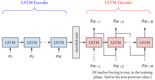
Figure 9: LSTM encoder-decoder architecture.

Appendix G Additional Results: Average Forecasts

Business-aware forecasts are visualized in Figure 10.

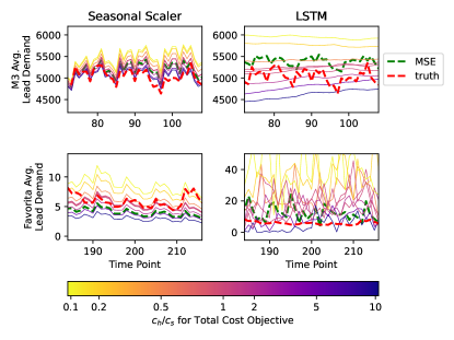
Figure 10: Forecasted and true lead demand, averaged across all series in M3 (first row) and Favorita (second row). True demand is the red dotted line, and forecasts from the MSE objective are the green dotted line. Forecasts from the TC objective are solid lines, for several unit cost tradeoffs—fixing $c_{v}=10^{-6}$ in the M3 dataset and $c_{v}=10^{-2}$ in the Favorita dataset, ratios of $c_{h}/c_{s}$ are indicated by line color.

Appendix H Additional Results: Relative Improvements with Different Tradeoffs

Figure 11: Improvements in total cost when using the TC objective vs. the MSE objective, under various cost tradeoffs. The first two columns correspond to different $c_{v}$’s on the M3 dataset, and the second two columns correspond to different $c_{v}$’s on the Favorita dataset. Radius is ten times the relative proportional improvement.

Bibliography

- Ahmed et al., (2020) Ahmed, R., Sreeram, V., Mishra, Y., and Arif, M. (2020). A review and evaluation of the state-of-the-art in pv solar power forecasting: Techniques and optimization. Renewable and Sustainable Energy Reviews, 124:109792.
- Ali and Yaman, (2013) Ali, Ö. G. and Yaman, K. (2013). Selecting rows and columns for training support vector regression models with large retail datasets. European Journal of Operational Research, 226(3):471–480.
- Assimakopoulos and Nikolopoulos, (2000) Assimakopoulos, V. and Nikolopoulos, K. (2000). The theta model: a decomposition approach to forecasting. International Journal of Forecasting, 16(4):521–530. The M3- Competition.
- Bai et al., (2018) Bai, S., Kolter, J. Z., and Koltun, V. (2018). An empirical evaluation of generic convolutional and recurrent networks for sequence modeling. arXiv preprint arXiv:1803.01271.
- Ban and Rudin, (2019) Ban, G.-Y. and Rudin, C. (2019). The big data newsvendor: Practical insights from machine learning. Operations Research, 67(1):90–108.
- Bertsimas and Thiele, (2005) Bertsimas, D. and Thiele, A. (2005). A data-driven approach to newsvendor problems. Working Papere, Massachusetts Institute of Technology, 51.
- Böse et al., (2017) Böse, J.-H., Flunkert, V., Gasthaus, J., Januschowski, T., Lange, D., Salinas, D., Schelter, S., Seeger, M., and Wang, Y. (2017). Probabilistic demand forecasting at scale. Proc. VLDB Endow., 10(12):1694–1705.
- Box et al., (2015) Box, G. E., Jenkins, G. M., Reinsel, G. C., and Ljung, G. M. (2015). Time series analysis: forecasting and control. John Wiley & Sons.
- Challu et al., (2022) Challu, C., Olivares, K. G., Oreshkin, B. N., Garza, F., Mergenthaler-Canseco, M., and Dubrawski, A. (2022). N-hits: Neural hierarchical interpolation for time series forecasting. arXiv preprint arXiv:2201.12886.
- Cheng et al., (2021) Cheng, C., Zhou, H., Weiss, J. C., and Lipton, Z. C. (2021). Unpacking the drop in covid-19 case fatality rates: A study of national and florida line-level data. In AMIA Annual Symposium Proceedings, volume 2021, page 285. American Medical Informatics Association.
- Chopra et al., (2007) Chopra, S., Meindl, P., and Kalra, D. V. (2007). Supply Chain Management by Pearson. Pearson Education India.
- Dai et al., (2021) Dai, H., Xue, Y., Syed, Z., Schuurmans, D., and Dai, B. (2021). Neural stochastic dual dynamic programming. arXiv preprint arXiv:2112.00874.
- Dhond et al., (2000) Dhond, A., Gupta, A., and Vadhavkar, S. (2000). Data mining techniques for optimizing inventories for electronic commerce. In Proceedings of the sixth ACM SIGKDD international conference on Knowledge discovery and data mining, pages 480–486.
- Donkor et al., (2014) Donkor, E. A., Mazzuchi, T. A., Soyer, R., and Alan Roberson, J. (2014). Urban water demand forecasting: review of methods and models. Journal of Water Resources Planning and Management, 140(2):146–159.
- Donti and Kolter, (2021) Donti, P. L. and Kolter, J. Z. (2021). Machine learning for sustainable energy systems. Annual Review of Environment and Resources, 46:719–747.
- Eilon and Elmaleh, (1968) Eilon, S. and Elmaleh, J. (1968). An evaluation of alternative inventory control policies. International Journal of Production Research, 7(1):1–14.
- Elliott and Timmermann, (2016) Elliott, G. and Timmermann, A. (2016). Forecasting in economics and finance. Annual Review of Economics, 8:81–110.
- Fan et al., (2019) Fan, C., Zhang, Y., Pan, Y., Li, X., Zhang, C., Yuan, R., Wu, D., Wang, W., Pei, J., and Huang, H. (2019). Multi-horizon time series forecasting with temporal attention learning. In Proceedings of the 25th ACM SIGKDD International conference on knowledge discovery & data mining, pages 2527–2535.
- Favorita, (2017) Favorita (2017). Corporación favorita grocery sales forecasting.
- Ferreira et al., (2016) Ferreira, K. J., Lee, B. H. A., and Simchi-Levi, D. (2016). Analytics for an online retailer: Demand forecasting and price optimization. Manufacturing & service operations management, 18(1):69–88.
- Fildes et al., (2022) Fildes, R., Ma, S., and Kolassa, S. (2022). Retail forecasting: Research and practice. International Journal of Forecasting, 38(4):1283–1318.
- Gardner Jr, (1985) Gardner Jr, E. S. (1985). Exponential smoothing: The state of the art. Journal of forecasting, 4(1):1–28.
- Ghalehkhondabi et al., (2017) Ghalehkhondabi, I., Ardjmand, E., Weckman, G. R., and Young, W. A. (2017). An overview of energy demand forecasting methods published in 2005–2015. Energy Systems, 8:411–447.
- Gilbert, (2005) Gilbert, K. (2005). An arima supply chain model. Management Science, 51(2):305–310.
- Hochreiter and Schmidhuber, (1997) Hochreiter, S. and Schmidhuber, J. (1997). Long short-term memory. Neural computation, 9(8):1735–1780.
- Hyndman and Billah, (2003) Hyndman, R. J. and Billah, B. (2003). Unmasking the theta method. International Journal of Forecasting, 19(2):287–290.
- Jones et al., (2009) Jones, S. S., Evans, R. S., Allen, T. L., Thomas, A., Haug, P. J., Welch, S. J., and Snow, G. L. (2009). A multivariate time series approach to modeling and forecasting demand in the emergency department. Journal of biomedical informatics, 42(1):123–139.
- Lee et al., (1997) Lee, H. L., Padmanabhan, V., and Whang, S. (1997). The bullwhip effect in supply chains1. Sloan Management Review, 38(3):93–102.
- Li et al., (2019) Li, S., Jin, X., Xuan, Y., Zhou, X., Chen, W., Wang, Y.-X., and Yan, X. (2019). Enhancing the locality and breaking the memory bottleneck of transformer on time series forecasting. Advances in neural information processing systems, 32.
- Lim et al., (2021) Lim, B., Arık, S. O., Loeff, N., and Pfister, T. (2021). Temporal fusion transformers for interpretable multi-horizon time series forecasting. International Journal of Forecasting, 37(4):1748–1764.
- Makridakis and Hibon, (1997) Makridakis, S. and Hibon, M. (1997). Arma models and the box–jenkins methodology. Journal of forecasting, 16(3):147–163.
- (32) Makridakis, S. and Hibon, M. (2000a). The m3-competition: results, conclusions and implications. International Journal of Forecasting, 16(4):451–476. The M3- Competition.
- (33) Makridakis, S. and Hibon, M. (2000b). The M3-Competition: results, conclusions and implications. International Journal of Forecasting, 16(4):451–476.
- Makridakis et al., (2020) Makridakis, S., Spiliotis, E., and Assimakopoulos, V. (2020). The m4 competition: 100,000 time series and 61 forecasting methods. International Journal of Forecasting, 36(1):54–74. M4 Competition.
- Makridakis et al., (2022) Makridakis, S., Spiliotis, E., and Assimakopoulos, V. (2022). M5 accuracy competition: Results, findings, and conclusions. International Journal of Forecasting, 38(4):1346–1364. Special Issue: M5 competition.
- Oord et al., (2016) Oord, A. v. d., Dieleman, S., Zen, H., Simonyan, K., Vinyals, O., Graves, A., Kalchbrenner, N., Senior, A., and Kavukcuoglu, K. (2016). Wavenet: A generative model for raw audio. arXiv preprint arXiv:1609.03499.
- Oreshkin et al., (2019) Oreshkin, B. N., Carpov, D., Chapados, N., and Bengio, Y. (2019). N-beats: Neural basis expansion analysis for interpretable time series forecasting. arXiv preprint arXiv:1905.10437.
- Oroojlooyjadid et al., (2017) Oroojlooyjadid, A., Nazari, M., Snyder, L., and Takáč, M. (2017). A deep q-network for the beer game: A reinforcement learning algorithm to solve inventory optimization problems. arXiv preprint arXiv:1708.05924, 5.
- Oroojlooyjadid et al., (2020) Oroojlooyjadid, A., Snyder, L. V., and Takáč, M. (2020). Applying deep learning to the newsvendor problem. IISE Transactions, 52(4):444–463.
- Pascanu et al., (2013) Pascanu, R., Mikolov, T., and Bengio, Y. (2013). On the difficulty of training recurrent neural networks. In International conference on machine learning, pages 1310–1318. Pmlr.
- Petropoulos et al., (2019) Petropoulos, F., Wang, X., and Disney, S. M. (2019). The inventory performance of forecasting methods: Evidence from the m3 competition data. International Journal of Forecasting, 35(1):251–265. Special Section: Supply Chain Forecasting.
- Petruzzi and Dada, (1999) Petruzzi, N. C. and Dada, M. (1999). Pricing and the newsvendor problem: A review with extensions. Operations research, 47(2):183–194.
- Qi et al., (2023) Qi, M., Shi, Y., Qi, Y., Ma, C., Yuan, R., Wu, D., and Shen, Z.-J. (2023). A practical end-to-end inventory management model with deep learning. Management Science, 69(2):759–773.
- Rangapuram et al., (2018) Rangapuram, S. S., Seeger, M. W., Gasthaus, J., Stella, L., Wang, Y., and Januschowski, T. (2018). Deep state space models for time series forecasting. Advances in neural information processing systems, 31.
- Reich et al., (2019) Reich, N. G., Brooks, L. C., Fox, S. J., Kandula, S., McGowan, C. J., Moore, E., Osthus, D., Ray, E. L., Tushar, A., Yamana, T. K., Biggerstaff, M., Johansson, M. A., Rosenfeld, R., and Shaman, J. (2019). A collaborative multiyear, multimodel assessment of seasonal influenza forecasting in the united states. Proceedings of the National Academy of Sciences, 116(8):3146–3154.
- Salinas et al., (2020) Salinas, D., Flunkert, V., Gasthaus, J., and Januschowski, T. (2020). Deepar: Probabilistic forecasting with autoregressive recurrent networks. International Journal of Forecasting, 36(3):1181–1191.
- Suganthi and Samuel, (2012) Suganthi, L. and Samuel, A. A. (2012). Energy models for demand forecasting—a review. Renewable and sustainable energy reviews, 16(2):1223–1240.
- Syntetos et al., (2009) Syntetos, A. A., Boylan, J. E., and Disney, S. M. (2009). Forecasting for inventory planning: a 50-year review. Journal of the Operational Research Society, 60:S149–S160.
- Taylor, (2000) Taylor, J. W. (2000). A quantile regression neural network approach to estimating the conditional density of multiperiod returns. Journal of forecasting, 19(4):299–311.
- Thomas, (2000) Thomas, L. C. (2000). A survey of credit and behavioural scoring: forecasting financial risk of lending to consumers. International journal of forecasting, 16(2):149–172.
- Turken et al., (2012) Turken, N., Tan, Y., Vakharia, A. J., Wang, L., Wang, R., and Yenipazarli, A. (2012). The multi-product newsvendor problem: Review, extensions, and directions for future research. Handbook of Newsvendor Problems: Models, Extensions and Applications, pages 3–39.
- Wang and Disney, (2016) Wang, X. and Disney, S. M. (2016). The bullwhip effect: Progress, trends and directions. European Journal of Operational Research, 250(3):691–701.
- Winters, (1960) Winters, P. R. (1960). Forecasting sales by exponentially weighted moving averages. Management science, 6(3):324–342.
- Yu et al., (2013) Yu, X., Qi, Z., and Zhao, Y. (2013). Support vector regression for newspaper/magazine sales forecasting. Procedia Computer Science, 17:1055–1062.