Electronic Structure Prediction of Multi-million Atom Systems Through Uncertainty Quantification Enabled Transfer Learning

Abstract

The ground state electron density — obtainable using Kohn-Sham Density Functional Theory (KS-DFT) simulations — contains a wealth of material information, making its prediction via machine learning (ML) models attractive. However, the computational expense of KS-DFT scales cubically with system size which tends to stymie training data generation, making it difficult to develop quantifiably accurate ML models that are applicable across many scales and system configurations. Here, we address this fundamental challenge by employing transfer learning to leverage the multi-scale nature of the training data. Our ML models employ descriptors involving simple scalar products, comprehensively sample system configurations through thermalization, and quantify uncertainty in electron density predictions using Bayesian neural networks. We show that our models incur significantly lower data generation costs while allowing confident — and when verifiable, accurate — predictions for a wide variety of bulk systems well beyond training, including systems with defects, different alloy compositions, and at unprecedented, multi-million-atom scales.

Figure 1: Overview of the present Machine Learning (ML) model. The first step is the training data generation via ab initio simulations shown by the arrow at the top. The second step is to generate atomic neighborhood descriptors $\mathbf{x}(i)$ for each grid point, $i$, in the training configurations. The third step is to create a probabilistic map (Bayesian Neural Network with a skip connection) from atomic neighborhood descriptors $\mathbf{x}(i)$ to the charge density at the corresponding grid point $\rho(i)$. The trained model is then used for inference which includes (i) descriptor generation for all grid points in the query configuration, (ii) forward propagation through the Bayesian Neural Network, and (iii) aggregation of the point-wise charge density $\rho(i)$ to obtain the charge density field $\rho$.

I Introduction

Over the past several decades, Density Functional Theory (DFT) calculations based on the Kohn-Sham formulation [1, 2] have emerged as a fundamental tool in the prediction of electronic structure. Today, they stand as the de facto workhorse of computational materials simulations [3, 4, 5, 6, 7, 8, 9, 10], offering broad applicability and versatility. Although formulated in terms of orbitals, the fundamental unknown in Kohn Sham Density Functional Theory (KS-DFT) is the electron density, from which many ground state material properties — including structural parameters, elastic constants, magnetic properties, phonons/vibrational spectra, etc., may be inferred. The ground state electron density is also the starting point for calculations of excited state phenomena, including those related to optical and transport properties [11, 12, 13].

In spite of their popularity, conventional KS-DFT calculations scale in a cubic manner with respect to the number of atoms within the simulation cell, making calculations of large and complex systems computationally burdensome. To address this challenge, a number of different approaches, which vary in their computational expense and their range of applicability, have been proposed over the years. Such techniques generally avoid explicit diagonalization of the Kohn-Sham Hamiltonian in favor of computing the single particle density matrix. Many of these methods are able to scale linearly with respect to the system size when bulk insulators are considered [14, 15, 16, 17, 18, 19], while others exhibit sub-quadratic scaling when used for calculations of low-dimensional materials (i.e., nanostructures)[20, 21, 22]. Contrary to these specialized approaches, there are only a handful of first-principles electronic structure calculation techniques that operate universally across bulk metallic, insulating, and semiconducting systems, while performing more favorably than traditional cubic scaling methods, (especially, close to room temperature). However, existing techniques in this category, e.g. [23, 24], tend to face convergence issues due to aggressive use of density matrix truncation, and in any case, have only been demonstrated for systems containing at most a few thousand atoms, due to their overall computational cost. Keeping these developments in mind, a separate thread of research has also explored reducing computational wall times by lowering the prefactor associated with the cubic cost of Hamiltonian diagonalization, while ensuring good parallel scalability of the methods on large scale high-performance computing platforms [25, 26, 27, 28]. In spite of demonstrations of these and related methods to study a few large example problems (e.g. [29, 30, 31]), their routine application to complex condensed matter systems, using modest, everyday computing resources appears infeasible.

The importance of being able to routinely predict the electronic structure of generic bulk materials, especially, metallic and semiconducting systems with a large number of representative atoms within the simulation cell, cannot be overemphasized. Computational techniques that can perform such calculations accurately and efficiently have the potential to unlock insights into a variety of materials phenomena and can lead to the guided design of new materials with optimized properties. Examples of materials problems where such computational techniques can push the state-of-the-art include elucidating the core structure of defects at realistic concentrations, the electronic and magnetic properties of disordered alloys and quasicrystals [32, 33, 34, 35], and the mechanical strength and failure characteristics of modern, compositionally complex refractory materials [36, 37]. Moreover, such techniques are also likely to carry over to the study of low dimensional matter and help unlock the complex electronic features of emergent materials such as van-der-Waals heterostructures [38] and moiré superlattices [39].

An attractive alternative path to overcoming the cubic scaling bottleneck of KS-DFT — one that has found much attention in recent years — is the use of Machine Learning (ML) models as surrogates [40]. Indeed, a significant amount of research has already been devoted to the development of ML models that predict the energies and forces of atomic configurations matching with KS-DFT calculations, thus spawning ML-based interatomic potentials that can be used for molecular dynamics calculations with ab initio accuracy [41, 42, 43, 44, 45, 46, 47]. Parallelly, researchers have also explored direct prediction of the ground state electron density via ML models trained on the self-consistent electron density obtained from KS-DFT simulations [48, 49, 50, 51, 52]. This latter approach is particularly appealing, since, in principle, the ground state density is rich in information that goes well beyond energies and atomic forces, and such details can often be extracted through simple post-processing steps. Having access to the electron density as an intermediate verifiable quantity is generally found to also increase the quality of ML predictions of various material properties [48, 53], and can allow training of additional ML models. Such models can use the density as a descriptor to predict specific quantities, such as defect properties of complex alloys [54, 55] and bonding information [56].

A key challenge in building surrogate models of the ground state electron density from KS-DFT calculations is the process of data generation itself, which can incur significant offline cost [57]. In recent work [53], we have demonstrated how this issue can be addressed for chiral nanomaterials [58]. For such forms of matter, the presence of underlying structural symmetries allows for significant dimensionality reduction of the predicted fields, and the use of specialized algorithms for ground state KS-DFT calculations [59, 60, 61, 62]. However, such strategies cannot be adopted for bulk materials with complex unit cells, as considered here. For generic bulk systems, due to the confining effects of periodic boundary conditions, small unit-cell simulations alone cannot represent a wide variety of configurations. To obtain ML models that can work equally well across scales and for a variety of configurations (e.g. defects [63, 64]), data from large systems is also essential. However, due to the aforementioned cubic scaling of KS-DFT calculations, it is relatively inexpensive to generate a lot of training data using small sized systems (say, a few tens of atoms), while larger systems (a few hundred atoms) are far more burdensome, stymieing the data generation process. Previous work on electron density prediction [51, 65] has been made possible by using data from large systems exclusively. However, this strategy is likely to fail when complex systems such as multi-principal element alloys are dealt with, due to the large computational cells required for such systems — especially while studying compositional variations, that are expected to increase the overall computational expense of the process significantly.

In this work, we propose a machine-learning model that accurately predicts the ground state electron density for bulk materials at any scale, while quantifying the associated uncertainties. Once trained, our model significantly outperforms conventional KS-DFT-based computations in terms of speed. To address the high cost of training data generation associated with KS-DFT simulations of larger systems — a key challenge in developing effective ML surrogates of KS-DFT — we adopt a transfer learning (TL) approach [66]. Thus, our model is first trained using a large quantity of cheaply generated data from simulations of small systems, following which, a part of the model is retrained using a small amount of data from simulations of a few large systems. This strategy significantly lowers the training cost of the ML model, without compromising its accuracy. Along with the predicted electron density fields, our model also produces a detailed spatial map of the uncertainty, that enables us to assess the confidence in our predictions for very large scale systems (thousands of atoms and beyond), for which direct validation via comparison against KS-DFT simulations data is not possible. The uncertainty quantification (UQ) properties of our models are achieved through the use of Bayesian Neural Networks (BNNs), which systematically obtain the variance in prediction through their stochastic parameters, and tend to regularize better than alternative approaches [67, 68, 69]. They allow us to systematically judge the generalizability of our ML model, and open the door to Active Learning approaches [70] that can be used to further reduce the work of data generation in the future.

To predict the electron density at a given point, the ML model encodes the local atomic neighborhood information in the form of descriptors, that are then fed as inputs to the BNN. Our neighborhood descriptors are rather simple: they include distance and angle information from nearby atoms in the form of scalar products and avoid basis selection and “handcrafted” descriptors adopted by other workers [71, 72, 73, 42]. Additionally, we have carried out a systematic algorithmic procedure to select the optimal set of descriptors, thus effectively addressing the challenge associated with the high dimensionality of the descriptor-space. To sample this descriptor space effectively, we have employed thermalization, i.e., ab initio molecular dynamics (AIMD) simulations at various temperatures, which has allowed us to carry out accurate predictions for systems far from training. Notably, the point-wise prediction of the electronic fields via the trained ML model, make this calculation scale linearly with respect to the system size, enabling a wide variety of calculations across scales.

In the following sections, we demonstrate the effectiveness of our model by predicting the ground state charge density for bulk metallic and semiconducting alloy systems. In particular, we present: (i) Predictions and error estimates for systems well beyond the training data, including systems with defects and varying alloy compositions; (ii) Demonstration of the effectiveness of the transfer learning approach; (iii) Uncertainty quantification capabilities of the model, and the decomposition of the uncertainty into epistemic and aleatoric parts; and (iv) Computational advantage of the model over conventional KS-DFT calculations, and the use of the model to predict the electron density of systems containing millions of atoms.

This contribution achieves several important technical milestones, including several “firsts”. These include: i) the first use of transfer learning to exploit the multiscale nature of electronic structure training data, thereby significantly reducing training data generation cost; (ii) effective use of thermalization to predict systems with localized and extended defects and for alloy compositions not included in training; (iii) demonstration of the use of simple scalar product descriptors for electronic field prediction; (iv) application of Bayesian Neural Networks to quantify uncertainty in electronic structure prediction, the analysis of uncertainty, and the use of this framework to gain confidence in the heuristic approaches adopted in the model development (i.e., points (i) and (ii) above); (v) the first systematic feature convergence analysis in the space of descriptors, for these types of models; and (vi) use of the framework to make computationally efficient, confident — and when verifiable, accurate — predictions for a wide variety of systems; in particular, making it possible to reliably calculate the electronic structure of multi-million atom systems on modest computing resources, for the first time.

(i) $1372$ atom aluminum simulation cell at $631$ K

(ii) 512 atoms Si_0.5Ge_0.5 simulation cell at 2300 K

Figure 2: Electron densities (a) calculated by DFT and (b) predicted by ML. The two-dimensional slice of (b) that has the highest mean squared error, as calculated by (c) DFT and predicted by (d) ML. (e) Corresponding absolute error in ML with respect to DFT. (i(f)-i(h)) Magnified view of the rectangular areas in (i(c)-i(e)) respectively.

II Results

(i) Aluminum system with defects

(ii) SiGe system with defects

Figure 3: (i) Electron density contours for aluminum systems with localized and extended defects — Left: calculated by DFT, Right: predicted by ML. i(a) (Top) Mono-vacancy in 256 atom aluminum system, (Bottom) Di-Vacancy in 108 atom aluminum system, i(b) (1 1 0) plane of a perfect screw dislocation in aluminum with Burgers vector $\frac{a_{0}}{2}[110]$, and line direction along $[110]$. The coordinate system was aligned along $[1\bar{1}2]$–$[\bar{1}11]$–$[110]$, i(c) (Top) (0 1 0) plane, (bottom) (0 0 1) plane of a $[001]$ symmetric tilt grain boundary ($0\degree$ inclination angle) in aluminum, i(d) Edge dislocation in aluminum with Burgers vector $\frac{a_{0}}{2}[110]$. The coordinate system was aligned along $[110]$–$[\bar{1}11]$–$[1\bar{1}2]$ and the dislocation was created by removing a half-plane of atoms below the glide plane.
(ii) Electron density contours and absolute error in ML for SiGe systems with ii(a-c) Si double vacancy defect in 512 atom system ii(d-f) Ge single vacancy defect in 216 atom system. Densities ii(a,d) calculated by DFT, ii(b,e) predicted by ML, and ii(c,f) error in ML predictions.
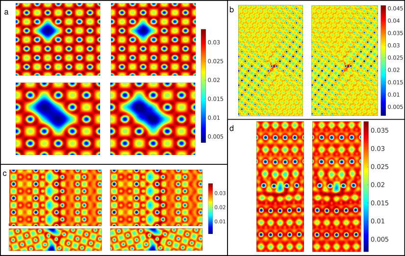
Note that the training data for the above systems did not include any defects.

Figure 4: A comparison of the accuracy in the prediction of the charge density (in terms of the L¹ norm per electron between $\rho^{\text{DFT}}$ and $\rho^{\text{scaled}}$), and the error (in Ha/atom) in the ground state total energy computed using $\rho^{\text{DFT}}$ and $\rho^{\text{scaled}}$, for Al (left), and SiGe (right) systems. $\rho^{\text{scaled}}$ is the scaled ML predicted electron density as given in Eq. 6. We observe that the errors are far better than chemical accuracy, i.e., errors below 1 kcal/mol or $1.6$ milli-Hartree/atom, for both systems, even while considering various types of defects and compositional variations. Note that for Si_xGe_1-x, we chose $x=0.4,0.45,0.55,0.6$.

Figure 5: The energy curve with respect to different lattice parameters for a $2\times 2\times 2$ (left) and $3\times 3\times 3$ (right) supercell of aluminum atoms. Overall, we see excellent agreement in the energies (well within chemical accuracy). The lattice parameter (related to the first derivative of the energy plot) calculated in each case agrees with the DFT-calculated lattice parameter to ${\cal O}(10^{-2})$ Bohr or better (i.e., it is accurate to a fraction of a percent). The bulk modulus calculated (related to the second derivative of the energy plot) from DFT data and ML predictions agree to within $1\%$. For the $3\times 3\times 3$ supercell, the bulk modulus calculated via DFT calculations is $76.39$ GPa, close to the experimental value of about $76$ GPa [74]. The value calculated from ML predictions is $75.80$ GPa.

(i) 1372 atom aluminum system

(ii) Si_0.4Ge_0.6 system

Figure 6: Uncertainty quantification for aluminum and SiGe systems. (a) ML prediction of the electron density, (b) Epistemic Uncertainty (c) Aleatoric Uncertainty (d) Total Uncertainty shown along the dotted line from the ML prediction slice. The uncertainty represents the bound $\pm 3\sigma_{total}$, where, $\sigma_{total}$ is the total uncertainty.

Figure 7: Uncertainty quantification for a 256 atom aluminum system with a mono vacancy defect. (a) ML prediction of the electron density shown on the defect plane, (b)) Epistemic uncertainty (c) Aleatoric uncertainty d) Uncertainty shown along the black dotted line from the ML prediction slice. The uncertainty represents the bound $\pm 3\sigma_{total}$, where, $\sigma_{total}$ is the total uncertainty. Note that the model used to make the predictions in (a-d) is not trained on the defect data, as opposed to the model used for (e), where defect data from the 108 atom aluminum system was used to train the model. The uncertainty and error at the location of the defect reduce with the addition of defect data in the training, as evident from (d) and (e).

In this section, we present electron density predictions by the proposed machine learning (ML) model for two types of bulk materials — pure aluminum and alloys of silicon-germanium. These serve as prototypical examples of metallic and covalently bonded semiconducting systems, respectively. These materials were chosen for their technological importance and because the nature of their electronic fields is quite distinct (see Fig. 14 in appendix), thus presenting distinct challenges to the ML model. Additionally, being metallic, the aluminum systems do not show simple localized electronic features often observed in insulators [75, 76], further complicating electron density prediction.

The overview of the present ML model is given in Fig. 1. The models are trained using a transfer learning approach, with thermalization used to sample a variety of system configurations. In the case of aluminum (Al), the model is trained initially on a 32-atom and subsequently on a 108-atom system. Corresponding system sizes for silicon germanium (SiGe) are 64 and 216 atoms respectively. Details of the ML model are provided in section IV.

We evaluate the performance of the ML models for a wide variety of test systems, which are by choice, well beyond the training data. This is ensured by choosing system sizes far beyond training, strained systems, systems containing defects, or alloy compositions not included in the training. We assess the accuracy of the ML models by comparing predicted electron density fields and ground state energies against DFT simulations. In addition, we quantify the uncertainty in the model’s predictions. We decompose the total uncertainty into two parts: “aleatoric” and “epistemic”. The first is a result of inherent variability in the data, while the second is a result of insufficient knowledge about the model parameters due to limited training data. The inherent variability in the data might arise due to approximations and round-off errors incurred in the DFT simulations and calculation of the ML model descriptors. On the other hand, the modeling uncertainty arises due to the lack of or incompleteness in the data. This lack of data is inevitable since it is impossible to exhaustively sample all possible atomic configurations during the data generation process. Decomposing the total uncertainty into these two parts helps distinguish the contributions of inherent randomness and incompleteness in the data to the total uncertainty. In the present work, a “heteroscedastic” noise model is used to compute the aleatoric uncertainty, which captures the spatial variation of the noise/variance in the data.

II.1 Error Estimation

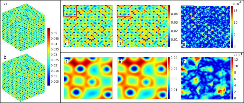
To evaluate the accuracy of the model, we calculated the Root Mean Squared Error (RMSE) for the entire dataset, including systems of the same size as the training data. For aluminum, the RMSE was determined to be $4.1\times 10^{-4}$, while for SiGe, it was $7.1\times 10^{-4}$, which shows an improvement over RMSE values for Al available in [51]. Additionally, the normalized RMSE is obtained by dividing the RMSE value by the range of respective $\rho$ values for aluminum and SiGe. The normalized RMSE for aluminum and SiGe was found to be $7.9\times 10^{-3}$ for both materials. To assess the generalizability of the model, we evaluate the accuracy of the ML model using systems much larger than those used in training, but accessible to DFT. We consider two prototypical systems, an Aluminium system having 1372 atoms (Fig. 2(i)) and a Silicon Germanium (Si${}_{0.5}\,$Ge_0.5) system having 512 atoms (Fig. 2(ii)). The model shows remarkable accuracy for both of these large systems. The RMSE is $3.8\times 10^{-4}$ and $7.1\times 10^{-4}$ for aluminum and SiGe respectively, which confirms the high accuracy of the model for system sizes beyond those used in training.

We now evaluate the performance of the ML model for systems containing extended and localized defects, although such systems were not used in training. We consider the following defects: mono-vacancies, di-vacancies, grain boundaries, edge, and screw dislocations for Al, and mono-vacancies and di-vacancies for SiGe. The electron density fields predicted by the ML models match with the DFT calculations extremely well, as shown in Figs. 3(i) and 3(ii). The error magnitudes (measured as the $L^{1}$ norm of the difference in electron density fields, per electron) are about $4\times 10^{-2}$ (see Fig. 4). We show in Section II.2 and the Appendix, that the model errors and uncertainty can be both brought down significantly, by including a single snapshot with defects, during training.

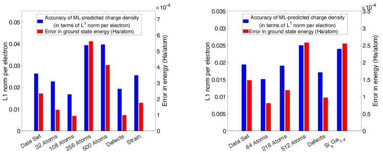
Another stringent test of the generalizability of the ML models is performed by investigating Si${}_{x}\,$Ge_1-x alloys, for $x\neq 0.5$. Although only equi-atomic alloy compositions (i.e., $x=0.5$) were used for training, the error in prediction (measured as the $L^{1}$ norm of the difference in electron density fields, per electron) is lower than $3\times 10^{-2}$ (see Fig. 4). We have also carried out tests with aluminum systems subjected to volumetric strains, for which the results were similarly good.

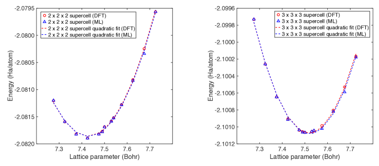
Our electron density errors are somewhat lower than compared to the earlier works [50, 51], At the same time, thanks to the sampling and transfer learning techniques adopted by us, the amount of time spent on DFT calculations used for producing the training data is also smaller. To further put into context the errors in the electron density, we evaluate the ground state energies from the charge densities predicted by the ML model through a postprocessing step and compare these with the true ground state energies computed via DFT. Details on the methodology for postprocessing can be found in the ‘Methods’ section, and a summary of our postprocessing results can be seen in Fig. 4, and in Tables 4 and 5, in the Appendix. On average, the errors are well within chemical accuracy for all systems considered and are generally ${\cal O}(10^{-4})$ Ha/atom, as seen in Fig. 4. Furthermore, not only are the energies accurate, but the derivatives of the energies, e.g., with respect to the supercell lattice parameter, are found to be quite accurate as well (see Fig. 5). This enables us to utilize the ML model to predict the optimum lattice parameter — which is related to the first derivative of the energy curve, and the bulk modulus — which is related to the second derivative of the energy curve, accurately. We observe that the lattice parameter is predicted accurately to a fraction of a percent, and the bulk modulus is predicted to within $1\%$ of the DFT value (which itself is close to experimental values [74]). Further details can be found in the Appendix. This demonstrates the utility of the ML models to predict not only the electron density but also other relevant physical properties.

Overall, the generalizability of our models is strongly suggestive that our use of thermalization to sample the space of atomic configurations, and the use of transfer-learning to limit training data generation of large systems are both very effective. We discuss uncertainties arising from the use of these strategies and due to the neural network model, in addition to the noise in the data, in the following sections.

(i) Aluminum

(ii) SiGe

Figure 8: Prediction of electronic structure for aluminum system containing $\approx$ $4.1$ million and $\text{Si}_{0.5}\text{Ge}_{0.5}$ system containing $\approx$ $1.4$ million atoms.

II.2 Uncertainty quantification

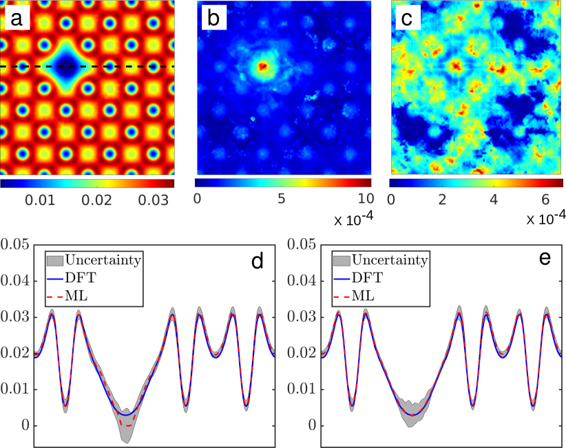
The present work uses a Bayesian Neural Network (BNN) and can thus systematically provide uncertainty estimates through the BNN’s stochastic parameters. Estimates of epistemic and aleatoric uncertainties for the following systems are shown: a defect-free Al system with $1372$ atoms (Fig. 6(i)), a $256$-atom Al system with a mono-vacancy (Fig. 7(a-d)), and a Si_0.4Ge_0.6 alloy (Fig. 6(ii)). Note, for the results in Fig. 7(a-d) the training data does not contain any systems having defects, and for the results in Fig. 6(ii) the training data contains only $50-50$ composition.

In these systems, the aleatoric uncertainty has the same order of magnitude as the epistemic uncertainty. This implies that the uncertainty due to the inherent randomness in the data is of a similar order as the modeling uncertainty. The aleatoric uncertainty is significantly higher near the nuclei (Fig. 6(i) and Fig. 6(ii)) and also higher near the vacancy (Fig 7). This indicates that the training data has high variability at those locations. The epistemic uncertainty is high near the nucleus (Fig. 6(i) and Fig. 6(ii)) since only a small fraction of grid points are adjacent to nuclei, resulting in the scarcity of training data for such points. The paucity of data near a nucleus is shown through the distribution of electron density in Fig. 14 in the Appendix. For the system with vacancy, the aleatoric uncertainty is higher in most regions, as shown in Fig. 7(c). However, the epistemic uncertainty is significantly higher only at the vacancy (Fig. 7 (b)), which might be attributed to the complete absence of data from systems with defects in the training.

To investigate the effect of adding data from systems with defects in the training, we added a single snapshot of $108$ atom aluminum simulation with mono vacancy defect to the training data. This reduces the error at the defect site significantly and also reduces the uncertainty (Fig. 7(e)). However, the uncertainty is still quite higher at the defect site because the data is biased against the defect site. That is, the amount of training data available at the defect site is much less than the data away from it. Thus, this analysis distinguishes uncertainty from inaccuracy.

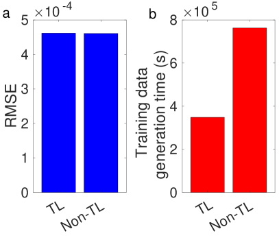
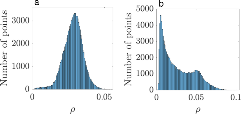
To investigate the effect of adding data from larger systems in training, we compare two models. The first model is trained with data from the $32$-atom system. The second model uses a transfer learning approach where it is initially trained using the data from the $32$-atom system and then a part of the model is retrained using data from the $108$-atom system. We observe a significant reduction in the error and in the epistemic uncertainty for the transfer learned model as compared to the one without transfer learning. The RMSE on the test system ($256$ atom) decreases by $50$% when the model is transfer learned using $108$ atom data. The addition of the $108$-atom system’s data to the training data decreases epistemic uncertainty as well since the $108$-atom system is less restricted by periodic boundary conditions than the $32$-atom system. Further, it is also statistically more similar to the larger systems used for testing as shown in Fig. 15. These findings demonstrate the effectiveness of the Bayesian Neural Network in pinpointing atomic arrangements or physical sites where more data is essential for enhancing the ML model’s performance. Additionally, they highlight its ability to measure biases in the training dataset. The total uncertainty in the predictions provides a confidence interval for the ML prediction. This analysis provides an upper bound of uncertainty arising out of two key heuristic strategies adopted in our ML model: data generation through thermalization of the systems and transfer learning.

II.3 Computational efficiency gains and confident prediction for unprecedented system sizes

The current ML model offers a huge computational advantage over traditional KS-DFT. While conventional KS-DFT calculations scale as ${\cal O}({N_{a}}^{3})$ with respect to the number of atoms $N_{a}$, our ML model scales linearly (i.e., ${\cal O}(N_{a})$), as shown in Fig. 18 of the Appendix. The computational costs for ML prediction and conventional KS-DFT calculations are starkly different, and even for systems with a few hundred atoms, the calculation wall times can be orders of magnitude lower for the ML model.

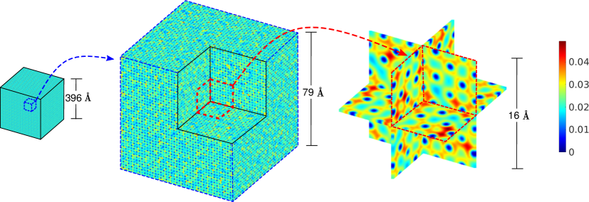
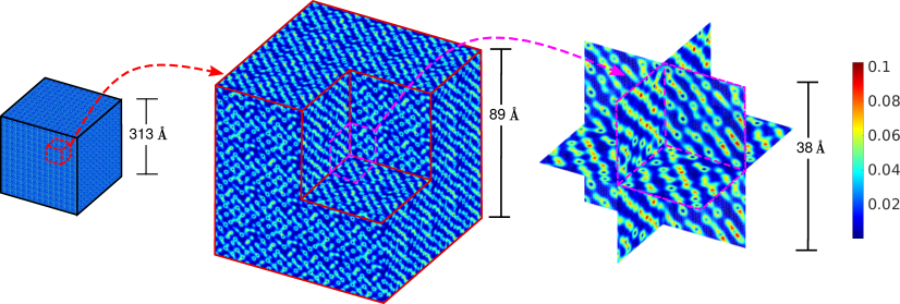
Taking advantage of this trend, the ML model can be used to predict the electronic structure for system sizes far beyond the reach of conventional calculation techniques, including systems containing millions of atoms, as demonstrated next. We anticipate that with suitable parallel programming strategies (the ML prediction process is embarrassingly parallel) and computational infrastructure, the present strategy can be used to predict the electronic structure of systems with hundreds of millions or even billions of atoms.

We show the electron densities, as calculated by our ML model, for a four million atom system of Al and a one million atom system of SiGe, in Figs. 8(i) and 8(ii) respectively. In addition to predicting electron densities, we also quantify uncertainties for these systems. We found that the ML model predicts larger systems with equally high certainty as smaller systems (see Fig. 13 of Appendix). The confidence interval obtained by the total uncertainty provides a route to assessing the reliability of predictions for these million atom systems for which KS-DFT calculations are simply not feasible.

II.4 Reduction of training data generation cost via transfer learning

One of the key challenges in developing an accurate ML model for electronic structure prediction is the high computational cost associated with the generation of the training data through KS-DFT, especially for predicting the electron density for systems across length-scales. A straightforward approach would involve data generation using sufficiently large systems wherein the electron density obtained from DFT is unaffected by the boundary constraints. However, simulations of larger bulk systems are significantly more expensive than smaller systems. To address this issue, we employed a transfer learning (TL) approach. We first trained the ML model on smaller systems and subsequently trained a part of the neural network using data from larger systems. This strategy allows us to obtain an efficient ML model that requires fewer simulations of expensive large-scale systems compared to what would have been otherwise required without the TL approach. The effectiveness of the TL approach stems from its ability to retain information from a large quantity of cheaper, smaller scale simulation data.

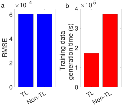
As an illustration of the above principles, we show in Fig. 9, the RMSE obtained on $256$ atom data (system larger than what was used in the training data) using the TL model and the non-TL model. We also show the time required to generate the training data for both models. For the Al systems, we trained the TL model with $32$-atom data first and then $108$-atom data. In contrast, the non-TL model was trained only on the $108$-atom data. Remarkably, the non-TL model requires significantly more $108$-atom data than the TL model to achieve a comparable RMSE on the 256-atom dataset. Moreover, the TL model’s training data generation time is approximately $55\%$ less than that of the non-TL model. This represents a substantial computational saving in developing the ML model for electronic structure prediction, making the transfer learning approach a valuable tool to expedite such model development. Similar savings in training data generation time were observed for SiGe as shown in Fig. 9. In the case of SiGe, the TL model was first trained using 64 atom data and then transfer learned using 216 atom data.

(i) Aluminum

(ii) SiGe

Figure 9: Models with Transfer Learning (TL) and without Transfer Learning (Non-TL): (a) Root mean square error (RMSE) on the test dataset and (b) Computational time to generate the training data. In the case of aluminum, the TL model is trained using 32 and 108 atom data. For SiGe, the TL model was trained using 64 and 216 atom data. In the case of aluminum, the non-TL model is trained using 108 atom data. Whereas, in the case of SiGe, the non-TL model is trained using 216 atom data.

III Discussions

We have developed an uncertainty quantification (UQ) enabled machine learning (ML) model that creates a map from the descriptors of atomic configurations to the electron densities. We use simple scalar product-based descriptors to represent the atomic neighborhood of a point in space. These descriptors, while being easy to compute, satisfy translational, rotational, and permutational invariances. In addition, they avoid any handcrafting. We systematically identify the optimal set of descriptors for a given dataset. Once trained, our model enables predictions across multiple length scales and supports embarrassingly parallel implementation. As far as we can tell, our work is the first attempt to systematically quantify uncertainties in ML predicted electron densities across different scales relevant to materials physics. To alleviate the high cost of training data generation via KS-DFT, we propose a two-pronged strategy: i) we use thermalization to comprehensively sample system configurations, leading to a highly transferable ML model; and ii) we employ transfer learning to train the model using a large amount of inexpensively generated data from small systems while retraining a part of the model using a small amount of data from more expensive calculations of larger systems. As a result of these strategies, the cost of training data generation is reduced by more than $50$%, while the models continue to be highly transferable across a large variety of material configurations. Our use of Bayesian Neural Networks (BNNs) allows the uncertainty associated with these aforementioned strategies to be accurately assessed, thus enabling confident predictions in scenarios involving millions of atoms, for which ground-truth data from conventional KS-DFT calculations is infeasible to obtain.

We demonstrate the versatility of the proposed machine learning models by accurately predicting the electron densities for multiple materials and configurations. We focus on bulk aluminum and Silicon-Germanium alloy systems. The ML model shows remarkable accuracy when compared with DFT calculations, even for systems having thousands of atoms. As mentioned above, the ML model also has excellent generalization capabilities, as it can predict electron densities for systems with localized and extended defects, and varying alloy compositions, even when the data from such systems were not included in the training. It is likely that the ensemble averaging over model parameters in the BNNs, along with comprehensive sampling of the descriptor space via system thermalization together contribute to the model generalization capabilities. Our findings also show a strong agreement between physical parameters calculated from the DFT and ML electron densities (e.g. lattice constants and bulk moduli).

To rigorously quantify uncertainties in the predicted electron density, we adopt a Bayesian approach. The uncertainty quantification by a Bayesian neural network (BNN) is mathematically well-founded and offers a more reliable measure of uncertainty in comparison to non-Bayesian approaches such as the method of ensemble averaging. Further, we can decompose the total uncertainty into aleatoric and epistemic parts. This decomposition allows us to distinguish and analyze the contributions to the uncertainty arising from (i) inherent noise in the training data (i.e. aleatoric uncertainty) and (ii) insufficient knowledge about the model parameters due to the lack of information in the training data (i.e. epistemic uncertainty). The aleatoric uncertainty or the noise in the data is considered irreducible, whereas the epistemic uncertainty can be reduced by collecting more training data. As mentioned earlier, the UQ capability of the model allows us to establish an upper bound on the uncertainty caused by two key heuristic strategies present in our ML model, namely, data generation via the thermalization of systems and transfer learning.

The reliability of the ML models is apparent from the low uncertainty of its prediction for systems across various length-scales and configurations. Furthermore, the magnitude of uncertainty for the million-atom systems is similar to that of smaller systems for which the accuracy of the ML model has been established. This allows us to have confidence in the ML predictions of systems involving multi-million atoms, which are far beyond the reach of conventional DFT calculations.

The ML model can achieve a remarkable speed-up of more than two orders of magnitude over DFT calculations, even for systems involving a few hundred atoms. As shown here, these computational efficiency gains by the ML model can be further pushed to regimes involving multi-million atoms, not accessible via conventional KS-DFT calculations.

In the future, we intend to leverage the uncertainty quantification aspects of this model to implement an active learning framework. This framework will enable us to selectively generate training data, reducing the necessity of extensive datasets and significantly lowering the computational cost associated with data generation. Moreover, we anticipate that the computational efficiencies offered via the transfer learning approach, are likely to be even more dramatic while considering more complex materials systems, e.g. compositionally complex alloys [77, 78].

IV Methods

IV.1 Ab Initio Molecular Dynamics

To generate training data for the model, Ab Initio Molecular Dynamics (AIMD) simulations were performed using the finite-difference based SPARC code [79, 80, 81]. We used the GGA PBE exchange-correlation functional [82] and ONCV pseudopotentials [83]. For aluminum, a mesh spacing of $0.25$ Bohrs was used while for SiGe, a mesh spacing of $0.4$ Bohrs was used. These parameters are more than sufficient to produce accurate energies and forces for the pseudopotentials chosen, as was determined through convergence tests. A tolerance of $10^{-6}$ was used for self-consistent field (SCF) convergence and the Periodic-Pulay [84] scheme was deployed for convergence acceleration. These parameters and pseudopotential choices were seen to produce the correct lattice parameters and bulk modulus values for the systems considered here, giving us confidence that the DFT data being produced is well rooted in the materials physics.

For AIMD runs, a standard NVT-Nosé Hoover thermostat [85] was used, and Fermi-Dirac smearing at an electronic temperature of $631.554$ K was applied. The time step between successive AIMD steps was $1$ femtosecond. The atomic configuration and the electron density of the system were captured at regular intervals, with sufficient temporal spacing between snapshots to avoid the collection of data from correlated atomic arrangements. To sample a larger subspace of realistic atomic configurations, we performed AIMD simulations at temperatures ranging from $315$ K to about twice the melting point of the system, i.e. $1866$ K for Al and $2600$ K for SiGe. Bulk disordered SiGe alloy systems were generated by assigning atoms randomly to each species, consistent with the composition.

We also generate DFT data for systems with defects and systems under strain, in order to demonstrate the ability of our ML model to predict unseen configurations. To this end, we tested the ML model on monovacancies and divacancies, edge and screw dislocations, and grain boundaries. For vacancy defects, we generated monovacancies by removing an atom from a random location, and divacancies by removing two random neighboring atoms before running AIMD simulations. Edge and screw dislocations for aluminum systems were generated using Atomsk [86]. Further details can be found in Fig. 3(i). Grain boundary configurations were obtained based on geometric considerations of the tilt angle — so that an overall periodic supercell could be obtained, and by removing extra atoms at the interface. For aluminum, we also tested an isotropic lattice compression and expansion of up to $5$%; these systems were generated by scaling the lattice vectors accordingly (while holding the fractional atomic coordinates fixed).

IV.2 Machine learning map for charge density prediction

Our ML model maps the coordinates $\{\textbf{R}_{I}\}_{I=1}^{N_{a}}$ and species (with atomic numbers $\{Z_{I}\}_{I=1}^{N_{a}}$) of the atoms, and a set of grid points $\{\textbf{r}_{i}\}_{i=1}^{N_{\text{grid}}}$ in a computational domain, to the electron density values at those grid points.

Here, $N_{a}$ and $N_{\text{grid}}$ refer to the number of atoms and the number of grid points, within the computational domain, respectively. We compute the aforementioned map in two steps. First, given the atomic coordinates and species information, we calculate atomic neighborhood descriptors for each grid point.

Second, a neural network is used to map the descriptors to the electron density at each grid point.

These two steps are discussed in more detail subsequently.

IV.3 Atomic neighborhood descriptors

In this work, we use a set of scalar product-based descriptors to encode the local atomic environment. The scalar product-based descriptors for the grid point at $\textbf{r}_{i}$ consist of distance between the grid point and the atoms at $\textbf{R}_{I}$; and the cosine of angle at the grid point $\textbf{r}_{i}$ made by the pair of atoms at $\textbf{R}_{I}$ and $\textbf{R}_{J}$. Here $i=1,\ldots,{N_{\text{grid}}}$ and $I,J=1,\ldots,N_{a}$. We refer to the collections of distances i.e., $||\textbf{r}_{i}-\textbf{R}_{I}||$ as set I descriptors, and the collections of the cosines of the angles i.e., $\frac{(\textbf{r}_{i}-\textbf{R}_{I})\cdot(\textbf{r}i-\textbf{R}_{J})}{||\textbf{r}_{i}-\textbf{R}_{I}||\,||\textbf{r}i-\textbf{R}_{J}||}$ are referred to as set II descriptors.

Higher order scalar products such as the scalar triple product, and the scalar quadruple product which involve more than two atoms at a time can also be considered. However, these additional scalar products are not included in the descriptor set in this work since they do not appear to increase the accuracy of predictions as elaborated in the Appendix.

IV.4 Selection of optimal set of descriptors

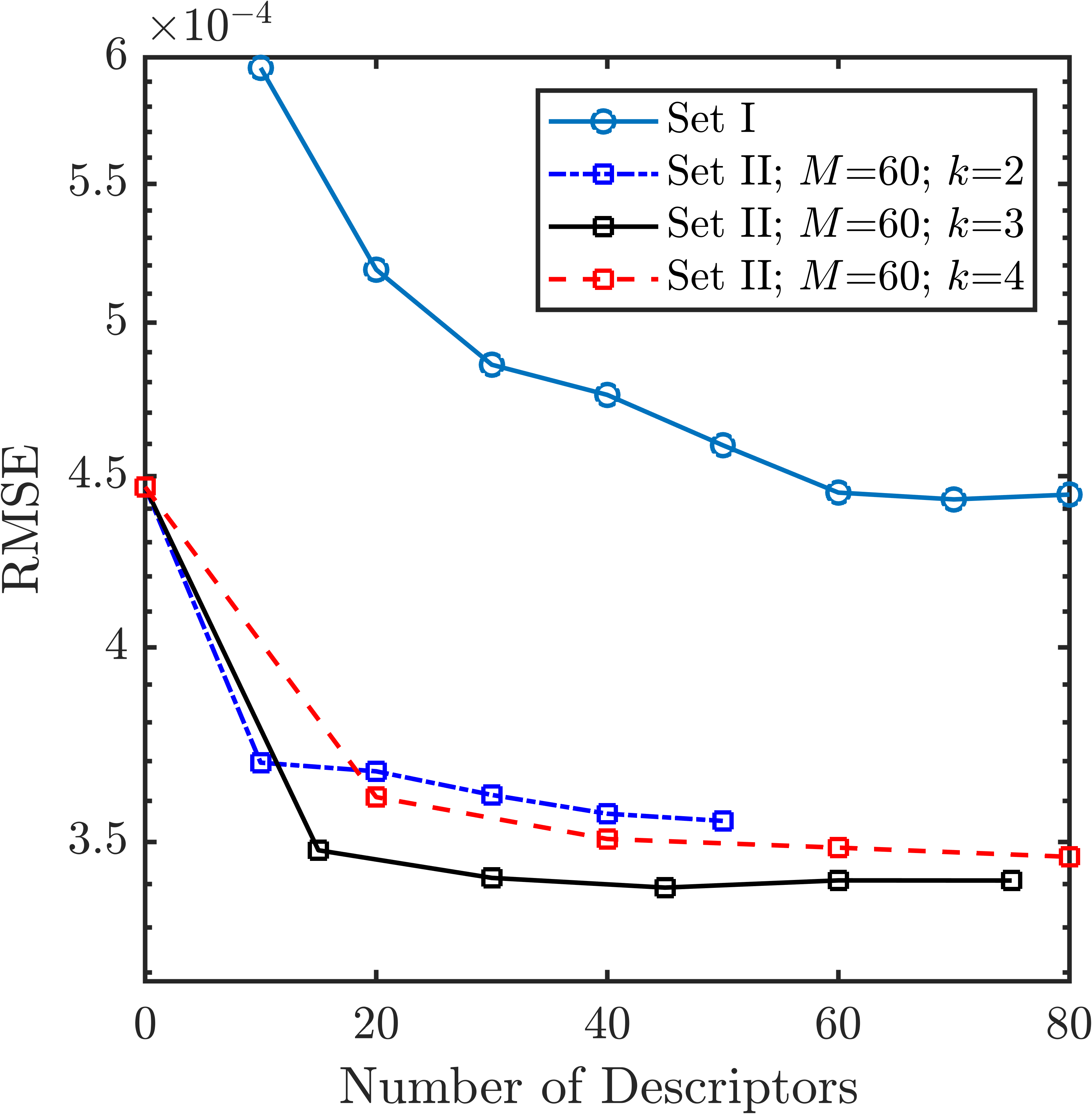
As has been pointed out by previous work on ML prediction of electronic structure [50, 51], the nearsightedness principle [87, 76] and screening effects [88] indicate that the electron density at a grid point has little influence from atoms sufficiently far away. This suggests that only descriptors arising from atoms close enough to a grid point need to be considered in the ML model, a fact which is commensurate with our findings in Fig. 10.

Using an excessive number of descriptors for specifying the atomic neighborhood can lead to high dimensionality of the space of descriptors, which in turn will require an enormous quantity of training data points to adequately cover the space (i.e., the curse of dimensionality [89, 90]). This adequate coverage is essential to accurately learn the ML map between descriptors and electron density. On the other hand, utilizing an insufficient number of descriptors can result in an inadequate representation of the atomic environments and lead to an inaccurate ML model.

Based on this rationale, we propose a procedure to select an optimal set of descriptors for a given atomic system. We select a set of $M$ ($M\leq N_{a}$) nearest atoms from the grid point to compute the descriptors and perform a convergence analysis to strike a balance between the aforementioned conditions to determine the optimal value of $M$.

For $M$ nearest atoms, we will have $N_{\text{set\,I}}$ distance descriptors, and $N_{\text{set\,II}}$ angle descriptors, with $N_{\text{set\,I}}=M$ and $N_{\text{set\,II}}\leq\,^{M}C_{2}$ .

The total number of descriptors is $N_{\text{desc}}=N_{\text{set I}}+N_{\text{set\,II}}$. To optimize $N_{\text{desc}}$, we first optimize $N_{\text{set I}}$, till the error converges as shown in Fig. 10. Subsequently, we optimize $N_{\text{set\,II}}$. To do this, we consider a nearer subset of atoms of size $M_{a}\leq M$, and for each of these $M_{a}$ atoms, we consider the angle subtended at the grid point, by the atoms and their $k$ nearest neighbors. This results in $N_{\text{set\,II}}=M_{a}\times k$, angle based descriptors, with $M_{a}$ and $k$ varied to yield the best results, as shown in Fig. 10. The pseudo-code for this process can be found in Algorithms V.3 and V.3. Further details on feature convergence analysis are provided in the Appendix.

Figure 10: Convergence of error with respect to the number of descriptors, shown for aluminum. The blue line shows the convergence with respect to $N_{\text{set\,I}}$, while the other three lines show convergence with respect to $N_{\text{set\,II}}$. The optimal $N_{\text{set\,I}}$ and $N_{\text{set\,II}}$ are obtained where their test RMSE values converge.

IV.5 Bayesian Neural Network

Bayesian Neural Networks (BNNs) have stochastic parameters in contrast to deterministic parameters used in conventional neural networks. BNNs provide a mathematically rigorous and efficient way to quantify uncertainties in their prediction.

We use a Bayesian neural network to estimate the probability $P(\rho|\mathbf{x},\mathcal{D})$ of the output electron density $\rho$ for a given input descriptor $\mathbf{x}\in\mathbb{R}^{N_{\text{desc}}}$ and training data set $\mathcal{D}=\{\mathbf{x}_{i},\rho_{i}\}_{i=1}^{N_{d}}$. The probability is evaluated as:

$$P(\rho|\mathbf{x},\mathcal{D})=\int_{\Omega_{w}}P(\rho|\mathbf{x},\mathbf{w})P(\mathbf{w}|\mathcal{D})d\mathbf{w}\,.$$ (1)

Here $\mathbf{w}\in\Omega_{w}$ is the set of parameters of the network and $N_{d}$ is the size of the training data set. Through this marginalization over parameters, a BNN provides a route to overcome modeling biases via averaging over an ensemble of networks. Given a prior distribution $P(\mathbf{w})$ on the parameters, the posterior distribution of the parameters $P(\mathbf{w}|\mathcal{D})$ are learned via the Bayes’ rule as $P(\mathbf{w}|\mathcal{D})=P(\mathcal{D}|\mathbf{w})P(\mathbf{w})/P(\mathcal{D})$, where $P(\mathcal{D}|\mathbf{w})$ is the likelihood of the data.

This posterior distribution of parameters $P(\mathbf{w}|\mathcal{D})$ is intractable since it involves the normalizing factor $P(\mathcal{D})$, which in turn is obtained via marginalization of the likelihood through a high dimensional integral. Therefore, it is approximated through techniques such as variational inference [91, 92, 93, 94, 67] or Markov Chain Monte Carlo methods [95, 96, 97]. In variational inference, as adopted here, a tractable distribution $q(\mathbf{w}|\bm{\theta})$ called the “variational posterior” is considered, which has parameters $\bm{\theta}$. For instance, if the variational posterior is a Gaussian distribution the corresponding parameters are its mean and standard deviation, $\bm{\theta}=(\bm{\mu}_{\theta},\bm{\sigma}_{\theta})$. The optimal value of parameters $\bm{\theta}$ is obtained by minimizing the statistical dissimilarity between the true and variational posterior distributions. The dissimilarity is measured through the KL divergence $\text{KL}\left[q(\mathbf{w}|\bm{\theta})\>||\>P(\mathbf{w}|\mathcal{D})\right]$. This yields the following optimization problem:

$$\begin{split}\bm{\theta}^{*}&=\arg\min_{\bm{\theta}}\text{KL}\left[q(\mathbf{w}|\bm{\theta})\>||\>P(\mathbf{w}|\mathcal{D})\right]\\ &=\arg\min_{\bm{\theta}}\int q(\mathbf{w}|\bm{\theta})\log\left[\frac{q(\mathbf{w}|\bm{\theta})}{P(\mathbf{w})P(\mathcal{D}|\mathbf{w})}P(\mathcal{D})\right]d\mathbf{w}\,.\end{split}$$ (2)

This leads to the following loss function for BNN that has to be minimized:

$$\mathcal{F}_{KL}(\mathcal{D},\bm{\theta})=\text{KL}\left[q(\mathbf{w}|\bm{\theta})\>||\>P(\mathbf{w})\right]-\mathbb{E}_{q(\mathbf{w}|\bm{\theta})}[\log P(\mathcal{D}|\mathbf{w})]\,.$$ (3)

This loss function balances the simplicity of the prior and the complexity of the data through its first and second terms respectively, yielding regularization [67, 68, 98].

Once the parameters $\bm{\theta}$ are learned, the BNNs can predict the charge density at any new input descriptor $\mathbf{x}$. In this work, the mean of the parameters ($\bm{\mu}_{\theta}$) are used to make point estimate predictions of the BNN.

IV.6 Uncertainty quantification

The variance in the output distribution $P(\rho|\mathbf{x},\mathcal{D})$ in Eq. (1) is the measure of uncertainty in the BNN’s prediction. Samples from this output distribution can be drawn in three steps: In the first step, a $j^{th}$ sample of the set of parameters, $\widehat{\mathbf{w}}_{j=1,...,N_{s}}$, is drawn from the variational posterior $q(\mathbf{w}|\bm{\theta})$ which approximates the posterior distribution of parameters $P(\mathbf{w}|\mathcal{D})$. Here, $N_{s}$ is the number of samples drawn from the variational posterior of parameters. In the second step, the sampled parameters are used to perform inference of the BNN ($f_{N}$) to obtain the $j^{th}$ prediction $\widehat{\rho}_{j}=f_{N}^{\mathbf{\widehat{w}_{j}}}(\mathbf{x})$. In the third step, the likelihood is assumed to be a Gaussian distribution: $P(\rho|\mathbf{x},\mathbf{\widehat{w}_{j}})=\mathcal{N}(\widehat{\rho}_{j},\sigma(\mathbf{x}))$, whose mean is given by the BNN’s prediction, $\widehat{\rho}_{j}$, and standard deviation by a heterogenous observation noise, $\sigma(\mathbf{x})$. A sample is drawn from this Gaussian distribution $\mathcal{N}(\widehat{\rho}_{j},\sigma(\mathbf{x}))$ that approximates a sample from the distribution $P(\rho|\mathbf{x},\mathcal{D})$. The total variance of such samples can be expressed as:

$$\text{var}(\rho)=\sigma^{2}(\mathbf{x})+\left[\frac{1}{N_{s}}\sum_{j=1}^{N_{s}}\left(\widehat{\rho}_{j}\right)^{2}-\left(\mathbb{E}(\widehat{\rho}_{j})\right)^{2}\right]\,.$$ (4)

Here, $\mathbb{E}(\widehat{\rho}_{j})=\frac{1}{N_{s}}\sum_{j=1}^{N_{s}}f_{N}^{\mathbf{\widehat{w}_{j}}}(\mathbf{x})$. The first term, $\sigma^{2}(\mathbf{x})$, in Eq. (4) is the aleatoric uncertainty that represents the inherent noise in the data and is considered irreducible. The second term (in the square brackets) in Eq. (4) is the epistemic uncertainty, that quantifies the modeling uncertainty.

In this work, the aleatoric uncertainty is learned via the BNN model along with the charge densities $\rho$. Therefore, for each input $\mathbf{x}$, the BNN learns two outputs: $f_{N}^{\mathbf{w}}(\mathbf{x})$ and $\sigma(\mathbf{x})$. For a Gaussian likelihood, the noise $\sigma$ is learned through the likelihood term of the loss function Eq. (3) following [99] as:

$$\log P(\mathcal{D}|\mathbf{w})=\sum_{i=1}^{N_{d}}-\frac{1}{2}\log\sigma_{i}^{2}-\frac{1}{2\sigma_{i}^{2}}(f_{N}^{\mathbf{w}}(\mathbf{x}_{i})-\rho_{i})^{2}\,.$$ (5)

Here, $N_{d}$ is the size of the training data set. The aleatoric uncertainty, $\sigma$, enables the loss to adapt to the data. The network learns to reduce the effect of erroneous labels by learning a higher value for $\sigma^{2}$, which makes the network more robust or less susceptible to noise. On the other hand, the model is penalized for predicting high uncertainties for all points through the $\log\sigma^{2}$ term.

The epistemic uncertainty is computed by evaluating the second term of Eq.(4), via sampling $\mathbf{\widehat{w}_{j}}$ from the variational posterior.

IV.7 Transfer Learning using multi-scale data

Conventional DFT simulations for smaller systems are considerably cheaper than those for larger systems, as the computational cost scales cubically with the number of atoms present in the simulation cell. However, the ML models cannot be trained using simulation data from small systems alone. This is because, smaller systems are far more constrained in the number of atomic configurations they can adopt, thus limiting their utility in simulating a wide variety of materials phenomena. Additionally, the electron density from simulations of smaller systems differs from that of larger systems, due to the effects of periodic boundary conditions.

To predict accurately across all length scales while reducing the cost of training data generation via DFT simulations, we use a transfer learning approach here. Transfer learning is a machine learning technique where a network, initially trained on a substantial amount of data, is later fine-tuned on a smaller dataset for a different task, with only the last few layers being updated while the earlier layers remain unaltered [66, 100].

The initial layers (called “frozen layers”) capture salient features of the inputs from the large dataset, while the re-trained layers act as decision-makers and adapt to the new problem.

Transfer learning has been used in training neural network potentials, first on Density Functional Theory (DFT) data, and subsequently using datasets generated using more accurate, but expensive quantum chemistry models [101]. However, its use in predicting electronic structure, particularly, by leveraging the multi-scale aspects of the problem — as done here — is novel. This approach allows us to make electron density predictions across scales, while significantly reducing the cost of training data generation.

In the case of aluminum, at first, we train the model using a large amount of data from DFT simulations of (smaller) $32$-atom systems. Subsequently, we freeze the initial one-third layers of the model and re-train the remaining layers of the model using a smaller amount ($40$%) of data from simulations of (larger) $108$-atom systems. Further training using data from larger bulk systems was not performed, since the procedure described above already provides good accuracy (Figs. 4,9), which we attribute to the statistical similarity of the electron density of $108$ atom systems and those with more atoms (Fig. 15). A similar transfer learning procedure is used for the SiGe model, where we initially train with data from $64$-atom systems and subsequently retrain using data from $216$-atom systems. Overall, due to the non-linear data generation cost using DFT simulations, the transfer learning approach reduces training data generation time by over $50$%.

IV.8 Postprocessing of ML predicted electron density

One way to test the accuracy of the ML models is to compute quantities of interest (such as the total ground state energy, exchange-correlation energy, and Fermi level) using the predicted electron density, $\rho^{\text{ML}}$. Although information about the total charge in the system is included in the prediction, it is generally good practice to first re-scale the electron density before postprocessing [56, 53], as follows:

$$\rho^{\text{scaled}}\left(\textbf{r}\right)=\rho^{\text{ML}}(\textbf{r})\frac{N_{\text{e}}}{\displaystyle\int_{\Omega}\rho^{\text{ML}}(\textbf{r})d\textbf{r}}\,.$$ (6)

Here, $\Omega$ is the periodic supercell used in the calculations, and $N_{\text{e}}$ is the number of electrons in the system. Using this scaled density, the Kohn-Sham Hamiltonian is set up within the SPARC code framework, which was also used for data generation via AIMD simulations [79, 80, 81]. A single step of diagonalization is then performed, and the energy of the system is computed using the Harris-Foulkes formula [102, 103]. The errors in predicting $\rho^{\text{ML}}(\textbf{r})$, and the ground state energy thus calculated, can be seen in Fig. 4. More detailed error values can be found in Table 4 and Table 5 in the Appendix.

V Appendix

Figure 11: Uncertainty quantification for a 256 atom aluminum system with mono vacancy defect. From left: i) ML prediction of the electron density shown on the defect plane, ii) Epistemic uncertainty iii) Aleatoric uncertainty iv) Uncertainty shown on the black dotted line from the ML prediction slice. The uncertainty represents the bound $\pm 3\sigma$, where, $\sigma$ is the total uncertainty.

Figure 12: Uncertainty quantification Si_0.5Ge_0.5 system containing 216 atoms. (a) ML prediction of the electron density, (b) Epistemic Uncertainty (c) Aleatoric Uncertainty (d) Total Uncertainty shown along the dotted line from the ML prediction slice. The uncertainty represents the bound $\pm 3\sigma_{total}$, where, $\sigma_{total}$ is the total uncertainty.

Figure 13: Total uncertainty for the Al system ($\sim 4.1$ million atoms) shown in Fig. 8(i) (left) and SiGe system ($\sim 1.4$ million atoms) shown in Fig. 8(ii) (right).

Figure 14: Histogram showing the distribution of charge density ($\rho$) for (a) aluminum and (b) SiGe.

Figure 15: (a-d) Comparison of the histograms of electron density obtained for a $1372$ atom aluminum system, with that obtained from smaller systems. The shaded green area shows the difference between the histograms. e) KL divergence of the distributions of electron densities represented by the histograms in a-d for $32$, $108$, $256$, and $500$ atom systems with respect to the $1372$ atom system. The KL divergence plot shows that the statistical dissimilarity between the electron density distribution of the largest system ($1372$ atom) and the rest of the systems ($32$, $108$, $256$, and $500$ atoms) decreases with the system size. For training the ML model, $32$ and $108$ atom systems are used, which provides desirable accuracy on the three testing systems ($256$, $500$ and $1372$ atom systems).

V.1 Efficient generation of atomic neighborhood descriptors

The atomic neighborhood descriptors to encode the atomic neighborhood of the grid point are $||\textbf{r}_{i}-\textbf{R}_{J}||$ and $\frac{(\textbf{r}_{i}-\textbf{R}_{K})\cdot(\textbf{r}i-\textbf{R}_{S})}{||\textbf{r}_{i}-\textbf{R}_{K}||\,||\textbf{r}i-\textbf{R}_{S}||}$, as described in the section IV. Our implementation of descriptor generation employs a tree data structure to reduce computational complexity and is outlined as a pseudocode in Algorithm V.1.

The descriptors described above satisfy the following conditions outlined in [71] and [104]: (i) invariance with respect to rotations and translations of the system (ii) invariance with respect to the permutation of atomic indices, i.e., the descriptors are independent of the enumeration of the atoms. (iii) for a given atomic neighborhood, the descriptors are unique. (iv) the descriptors encode the atomic neighborhood effectively while keeping the overall count low. (v) the descriptors generation process is computationally inexpensive and uses standard linear algebra operations.

Generation of Descriptors

$M$ = Number of nearest neighbor atoms to compute distances

$M_{a}$ = Number of nearest neighbor atoms to compute angles

$k$ = Number of angles obtained for each $M_{a}$ atoms

Build supercell by extending unit cell in all directions

KDTree = K-D tree for atoms in supercell

for $\mathbf{g}$ do $\triangleright$ $\mathbf{g}$: grid point

     $D\leftarrow$ distances to $M$ nearest atoms from $\mathbf{g}$ using K-D tree

     for $j=1$ to $M_{a}$ do

         $\mathbf{a}_{i}$ $\triangleright$ coordinates of $i^{th}$ nearest atom from $g$ using K-D tree

         $\mathbf{v}_{1}\leftarrow\mathbf{a}_{i}-\mathbf{g}$

         for $j=1$ to $k$ do

              $\mathbf{A}_{j}$ $\triangleright$ coordinates of $j^{th}$ nearest atom from $\mathbf{a}_{i}$

              $\mathbf{v}_{2}\leftarrow\mathbf{A}_{j}-\mathbf{g}$

              $\mathcal{A}_{ij}\leftarrow\frac{\mathbf{v}_{1}\cdot\mathbf{v}_{2}}{||\mathbf{v}_{1}||\;||\mathbf{v}_{2}||}$

         end for

     end for

     $\mathcal{A}\leftarrow$ flatten($\mathcal{A}$)

     descriptors $\leftarrow$ [$D,\mathcal{A}$]

end for

Note: Inner two for loops are vectorized and Outermost for is parallelized in the implementation

Descriptors are obtained by implementing a parallelized version of Algorithm V.1. In the case of SiGe systems, instead of explicitly encoding the species information, we follow [51] and concatenate the descriptors obtained for Si and Ge, to form inputs to the neural network. To encode the relative placement of Si and Ge atoms with respect to each other, we also consider the cosine of angles between Si and Ge atoms formed at the grid point for the SiGe case.

V.2 Computational Efficiency

Computational time comparison between DFT calculation and ML prediction is given in tables 1 and 2 for aluminum and SiGe, respectively. DFT calculations were performed using CPUs, whereas the ML predictions used a combination of GPU (inference step) and CPU (descriptor generation) resources. Within the ML model, the descriptor calculation consumes most of the computational effort ($\approx 94\%$) and the inference step takes up the rest of the time. However, the wall time for descriptor generation can be reduced by parallelization and we observe $66.6$% strong scaling for $64$ processors on NERSC Perlmutter CPUs.

The DFT and ML calculations presented in this work were performed through a combination of resources, namely, desktop workstations, the Hoffman2 cluster at UCLA’s Institute of Digital Research and Education (IDRE), the Applied Computing GPU cluster at MTU, and NERSC’s supercomputer, Perlmutter. Every compute node of the Hoffman2 cluster has two $18$-core Intel Xeon Gold 6140 processors ($24.75$ MB L3 cache, clock speed of $2.3$ GHz), $192$ GB of RAM and local SSD storage. Every compute node on Perlmutter has a $64$-core AMD EPYC 7763 processor ($256$ MB L3 cache, clock speed of $2.45$ GHz), $512$ GB of RAM and local SSD storage. The GPU resources on Perlmutter consist of NVIDIA A100 Tensor Core GPUs. The GPU nodes used at UCLA and MTU consist of Tesla V100 GPUs.

Large system calculations: We present electron density calculation for Al and SiGe systems, each with an excess of a million atoms, in Fig. 8(i) and Fig. 8(ii), respectively. To predict the charge density while avoiding memory overload issues, we partition these multi-million atom systems into smaller systems, while retaining the atomic neighborhood information consistent with the larger original systems. In the case of aluminum, we break down the $4.1$M atom system into smaller units comprising $1372$ atoms and a grid consisting of $175^{3}$ points. Computation of descriptors for this $1372$-atom chunk takes approximately $34.72$ seconds on a desktop workstation system equipped with a $36$-core Intel(R) Xeon(R) Gold 5220 CPU @ 2.20GHz. Subsequently, the charge density prediction requires approximately $1.6$ seconds on an Nvidia V100 GPU. Overall, the charge density prediction for the $4.1$M Al system takes around $30.72$ hours of wall time on combined CPU and GPU resources.

Analogously, for SiGe, we partition the $1.4$M atom system into smaller systems composed of $1000$ atoms and a grid with dimensions of $132^{3}$ points. The computation of descriptors for this $1000$-atom SiGe chunk requires $22.17$ seconds on the aforementioned desktop system. The subsequent charge density prediction takes approximately $1.1$ seconds. Overall, it takes around $6.8$ hours of wall time on combined CPU and GPU resources, to predict the electron density of the SiGe system with $1.4$M atoms.

Thus, the techniques described here make it possible to routinely predict the electronic structure of systems at unprecedented scales, while using only modest resources on standard desktop systems.

Number of Atoms		32	108	256	500
DFT Time (CPU)		466	11560	112894	245798
ML Time	Descriptor Generation	43.25	151.52	367.54	739.58
	$\rho$ Prediction (CPU)	2.76	9.67	23.46	47.20
	$\rho$ Prediction (GPU)	0.60	0.64	0.75	0.99
	Total (With GPU)	43.85	152.16	368.29	740.57
DFT time / Total ML time		10.63	75.97	306.53	331.90

Table 1: Comparison of DFT and ML wall times for prediction of electron density for an aluminum system. All times are in seconds. The DFT calculations were performed on Hoffman CPUs, ML descriptor generation was done on Hoffman CPUs, and the ML inference was performed on Tesla V100 GPUs.

Number of Atoms		64	216	512	1000
DFT Time		185	4774	51247	281766
ML Time	Descriptor Generation	38.82	115.23	291.45	611.2
	$\rho$ Prediction (CPU)	2.22	7.37	17.37	33.05
	$\rho$ Prediction (GPU)	0.50	0.62	0.75	0.89
	Total (With GPU)	39.32	115.85	292.20	612.09
DFT time / Total ML time		4.70	41.21	175.38	460.33

Table 2: Comparison of DFT and ML wall times for prediction of electron density for a SiGe system. All times are in seconds. The DFT calculations were performed on Perlmutter CPUs, ML descriptor generation was done on Perlmutter CPUs and the ML inference was performed on Tesla V100 GPUs.

V.3 Feature Convergence Analysis

Algorithm V.3 and Algorithm V.3 describe the process used to obtain the optimal number of descriptors. In algorithm V.3 only distances (set I) are considered as descriptors. The size of the set I (i.e. $M$) is selected for which the RMSE for the test dataset converges.

Optimal nearest neighbors

$M=0$ $\triangleright$ Initialization

$\epsilon_{0}=\epsilon_{-m}=\delta_{1}=\delta_{2}=$ A large number $\triangleright$ Initialization

$\eta$ = tolerance in RMSE

while  $\delta_{1}\geq\eta\;\&\;\delta_{2}\geq\eta$  do

     $M=M+m$ $\triangleright$ Increase $M$ by $m\in\mathbb{Z^{+}}$

     $N_{\text{set\,I}}\leftarrow M$ $\triangleright$ $M$ nearest atoms

     $N\leftarrow N_{\text{set\,I}}$ $\triangleright$ Only set I descriptors

     Compute $N$ descriptors

     Train $f_{N}$ $\triangleright$ Train the BNN

     $\epsilon_{M}\leftarrow$ RMSE $\triangleright$ Compute RMSE

     $\delta_{1}\leftarrow|\epsilon_{M}-\epsilon_{M-m}|$

     $\delta_{2}\leftarrow|\epsilon_{M}-\epsilon_{M-2m}|\,$

end while

$M=M-2m$

As an illustration, for the aluminum systems, following algorithm V.3 we use an increment of $m=10$. The algorithm converges to $M=60$ as seen in Fig. 10. Therefore, the set I consists of $60$ descriptors. Next, Set II descriptors consist of angles subtended at the grid point by a pair of atoms taken from the set of $M$ neighboring atoms in the set I determined by algorithm V.3. Each pair of the neighboring atoms forms an angle at the grid point, yielding a total of $M(M-1)/2$ angles, which quickly becomes computationally intractable with increasing $M$. To alleviate this issue, we reduce the number of Set II descriptors by eliminating large angles, which are not expected to play a significant role. This amounts to choosing angles originating from $M_{a}<M$ atoms closest to the grid point, and the $k-$ nearest neighbors of each of these atoms. This yields a total of $M_{a}\times k$ angle descriptors. For various fixed values of $k$, we iteratively choose $M_{a}$ till the RMSE over the test dataset converges (Fig. 10).

Optimal number of angles

$k=0$ $\triangleright$ Initialization

$\epsilon_{0}=\epsilon_{-m}=\delta_{1}=\delta_{2}=\delta_{3}=$ A large number $\triangleright$ Initialization

$\eta$ = tolerance in RMSE

while  $\delta_{3}\geq\eta$  do

     $k=k+1$

     $M_{a}=0$

     while  $\delta_{1}\geq\eta\;\&\;\delta_{2}\geq\eta$  do

         $M_{a}=M_{a}+m_{a}$ $\triangleright$ Increase $M_{a}$ by $m_{a}\in\mathbb{Z^{+}}$

         $N_{\text{set\,II}}\leftarrow M_{a}\times k$ $\triangleright$ $k$ neighbors of each of $M_{a}$ nearest atoms

         $N\leftarrow N_{\text{set\,I}}+N_{\text{set\,II}}$ $\triangleright$ Number of total descriptors

         Compute $N$ descriptors

         Train $f_{N}$ $\triangleright$ Train the BNN

         $\epsilon_{M_{a}}\leftarrow$ RMSE $\triangleright$ Compute RMSE

         $\delta_{1}\leftarrow|\epsilon_{M_{a}}-\epsilon_{M_{a}-m_{a}}|$

         $\delta_{2}\leftarrow|\epsilon_{M_{a}}-\epsilon_{M_{a}-2m_{a}}|\,$

     end while

     $M_{a}=M_{a}-2m_{a}$

     $\epsilon^{\prime}_{k}\leftarrow\epsilon_{M_{a}}$

     $\delta_{3}\leftarrow|\epsilon^{\prime}_{k}-\epsilon^{\prime}_{k-1}|\,$

end while

$k=k-1$

Following algorithm V.3 we use an increment of $m=5$. Fig. 10 shows the convergence plot for angles for $k=2,3$, and $4$. For $M=60$, the RMSE value is the minimum for $k=3$. The RMSE value for $k=3$ converges at $M_{a}=15$, which results in a total of $M_{a}\times k=45$ angles. Therefore, set II consists of $45$ descriptors. To summarize, following the present feature selection strategy, the total number of descriptors used for the aluminum model is $N=N_{\text{set\,I}}+N_{\text{set\,II}}=105$.

We found that including scalar triple products and scalar quadruple products in the descriptor, in addition to the dot products, did not improve the accuracy of the ML model. To interpret why this is the case, we observe that the (normalized) scalar triple product can be interpreted in terms of the corner solid angle (polar sine function) of the parallelepiped generated by three vectors starting at the given grid point and ending at three atoms chosen in the neighborhood of the grid point. However, this quantity can also be calculated through the dot products between these vectors and is, therefore, already incorporated in the second set of descriptors. Therefore, the scalar triple product does not furnish any additional information. Similar arguments can be made for quadruple and higher products.

V.4 Details on Uncertainty Quantification

We provide additional results on uncertainty quantification (UQ) in this section. One of the key advantages of the inbuilt UQ capabilities of the present ML model is that it allows us to assess the model’s generalizability. To illustrate this, we consider systems with defects and varying alloy compositions. The uncertainty estimates of a model trained without any defect data in training are shown in Fig. 7. The model is more confident in its prediction of defects even if a small amount (single snapshot) of defect data is added in training. This is evident by comparing Fig. 11 and 7. This result is in agreement with the fact that unavailability or insufficient training data could yield high epistemic uncertainties at locations where such incompleteness of data exists. In addition to high uncertainty, the error at the defect location increases when data from systems with defects are not used in training. This implies a positive correspondence between error and uncertainty in the Bayesian neural network model. A similar effect of higher uncertainty for unknown compositions is observed for the SiGe systems. Since the model is trained only with data from SiGe systems with 50-50 composition, the uncertainties quantified for this composition shown in Fig. 12 is less in comparison to the prediction for 60-40 composition (Fig. 6(ii)). However, the uncertainty for the 60-40 composition is not significantly higher than the 50-50 composition, demonstrating the generalization capability of the ML model.

Results of uncertainty quantification $\approx$ 4.1 million atom aluminum system and $\approx$ 1.4 million atom SiGe system are shown in Fig.  13. With an increase in system size, we extrapolate farther away from the system size included in the training data. Despite this, the total uncertainty of millions of atom systems is similar to that of smaller systems. This implies that the model can predict systems with millions of atoms with the same level of confidence as smaller systems, which in turn assures the accuracy of the predictions.

We found that the ML model is less confident in predicting charge densities near the nucleus in comparison to the away from the nucleus for various systems, which is reflected in the high values of uncertainties at those locations. We attribute this to fewer grid points close to the nuclei, and the availability of more data away from them. This imbalance in the data is evident from the histograms for the distribution of charge densities shown in Fig. 14, where grid points with low values of the electron density — as is the case with points very close to the nuclei — are seen to be very few.

V.5 Details on the advantages of transfer learning

(i) Al system

(ii) SiGe System

Figure 16: Comparison of (a) error and (b) training data generation time between models with and without transfer learning.

Figure 17: (i) Decrease in error and uncertainty for a larger system (1372 atom) with transfer learning. Comparison is shown between predictions by a non-TL model trained using data only from the 32-atom system i(a-c) and a TL model trained by transfer learning using additional data from the 108-atom system i(d-f). The slice considered is shown in Fig. 6(i)(a). i(a and d) Error in ML prediction, i(b and e) Epistemic uncertainty, i(c and f) Total uncertainty along a line, as shown in Fig. 6(i)(a). Color bars are the same for i(a) and (c), and i(b) and (d). (ii) Bar plot showing a decrease in RMSE error and epistemic uncertainty. ii(a) The decrease in RMSE error is 56% and ii(b) the decrease in the mean epistemic uncertainty is 29%.

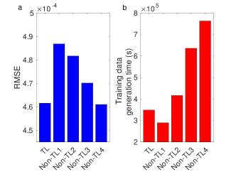
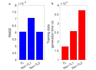
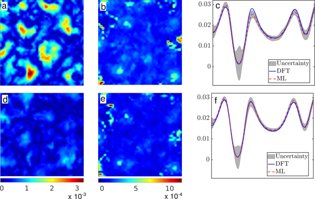
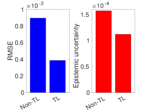
The transfer learning approach significantly reduces the root-mean-square error of a test dataset while costing much less computation for the training data generation as discussed in the main text. To depict this, a comparison of the transfer learned model with various non-transfer learned models is shown in Fig. 16.

We found that transfer learning helps to reduce the error and uncertainty in prediction for larger systems. By adding data from the $108$-atom systems in training, during the transfer learning approach, we significantly reduce the error (by 56%) and uncertainty (by 29%) of the predictions for a $1372$-atom test system, in comparison to a non-TL model trained using data only from the $32$-atom systems, as shown in Fig. 17.

Figure 18: Computational time comparison between DFT calculations and prediction via trained ML model. (Left) Aluminum, (Right) SiGe.

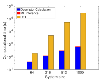
V.6 Bayesian Neural Network Details

Architecture: We use a Densenet [105] type architecture with three Dense blocks for the Bayesian Neural networks in this work. Each Dense block is composed of three hidden layers with $250$ nodes per layer and a GELU activation function [106]. The skip connections in the Densenet-type architecture are weighted by a trainable coefficient. These skip connections have multiple advantages. Firstly, they prevent gradients from diminishing significantly during backpropagation. Further, they facilitate improved feature propagation by allowing each layer to directly access the feature generated by previous layers. Finally, these skip connections promote feature reuse, thereby substantially reducing the number of parameters. Such skip connections have been used for electron density predictions in the literature [50].
Due to the stochastic weights of Bayesian neural networks, each weight is represented by its mean and standard deviation. Thus, the number of parameters in a Bayesian neural network is twice as compared to a deterministic network with the same architecture. In addition, the output of the Bayesian Neural networks used in this work has two neurons, one for predicting the charge density ($\rho$) and the other for predicting the aleatoric uncertainty ($\sigma$).

Training Details: The Adam optimizer [107] was used for training and the learning rate was set to $10^{-3}$ for all the networks used in this work. The training time for the Al and SiGe systems are presented in Table 3. All the Bayesian Neural networks are trained on NVIDIA A100 Tensor Core GPUs

The amount of data used in training for the two systems is as follows:

• Al: 127 snaps from 32 atom data and in addition 25 snaps from 108 atom data. The 108 atom data has $90\times 90\times 90$ grid points, while the 32 atom system has $60\times 60\times 60$ grid points.

• SiGe: 160 snaps of 64 atom data and in addition 30 snaps of 216 atom data. The 64 atom system has $53\times 53\times 53$ grid points, while the 216 atom system has $79\times 79\times 79$ grid points.

System	Size	Epochs	Training wall time (s)
			Per epoch	Total
Al	32	20	906	31060
	108	20	647
SiGe	64	20	651	18030
	216	10	501

Table 3: GPU Training times for the BNNs. The training was performed on the NVIDIA Tesla A100 GPU.

Validation and Testing Details: 20% of the data from the systems used for training is used as validation data. Testing is performed on systems that are larger than those used for generating the training data.

V.7 Postprocessing results for Al and SiGe

In table 4, we compare ground state energies for Al and SiGe systems. We see errors in the millihartree per atom, even in the presence of defects and some degree of compositional variations.

Case	Accuracy of	Ground-state	Exch. Corr.	Fermi	Max error in
	electron density	energy	energy	level	eigenvalue
	(L1 norm per electron)	(Ha/atom)	(Ha/atom)	(Ha)	(Ha)
Entire test data set	$2.62\times 10^{-2}$	$2.33\times 10^{-4}$	$4.36\times 10^{-4}$	$4.61\times 10^{-4}$	$4.58\times 10^{-3}$
Al ($32$ atoms)	$2.27\times 10^{-2}$	$1.30\times 10^{-4}$	$1.07\times 10^{-3}$	$9.80\times 10^{-4}$	$4.10\times 10^{-3}$
Al ($108$ atoms)	$1.67\times 10^{-2}$	$9.33\times 10^{-5}$	$9.82\times 10^{-5}$	$1.13\times 10^{-4}$	$1.87\times 10^{-3}$
Al ($256$ atoms)	$3.93\times 10^{-2}$	$5.60\times 10^{-4}$	$4.18\times 10^{-4}$	$2.03\times 10^{-4}$	$6.67\times 10^{-3}$
Al ($500$ atoms)	$3.96\times 10^{-2}$	$4.11\times 10^{-4}$	$2.41\times 10^{-4}$	$5.04\times 10^{-4}$	$8.52\times 10^{-3}$
Al vacancy defects	$1.92\times 10^{-2}$	$9.80\times 10^{-5}$	$1.42\times 10^{-4}$	$2.98\times 10^{-4}$	$3.85\times 10^{-3}$
Strain imposed Al	$2.54\times 10^{-2}$	$1.75\times 10^{-4}$	$8.91\times 10^{-4}$	$6.64\times 10^{-4}$	$3.11\times 10^{-3}$

Table 4: Accuracy of the ML predicted electron density in terms of the L¹ norm per electron, calculated as $\frac{1}{N_{\text{e}}}\times\displaystyle\int_{\Omega}\left|\rho^{\text{scaled}}(\textbf{r})-\rho^{\text{DFT}}(\textbf{r})\right|d\textbf{r}$, for various test cases for an FCC aluminum bulk system ($N_{\text{e}}$ is the number of electrons in the system). Also shown in the table are errors in the different energies as computed from $\rho^{\text{scaled}}$. The test data set for post-processing was chosen such that it covered examples from all system sizes, configurations, and temperatures. For calculating the relevant energies, $\rho^{\text{scaled}}$ was used as the initial guess for the electron density, and a single Hamiltonian diagonalization step was performed. Energies were then computed.

Case	Accuracy of	Ground-state	Exch. Corr.	Fermi	Max error in
	electron density	energy	energy	level	eigenvalue
	(L1 norm per electron)	(Ha/atom)	(Ha/atom)	(Ha)	(Ha)
Entire test data set	$1.93\times 10^{-2}$	$1.47\times 10^{-4}$	$9.34\times 10^{-4}$	$1.43\times 10^{-3}$	$7.29\times 10^{-3}$
Si_0.5Ge_0.5 ($64$ atoms)	$1.51\times 10^{-2}$	$8.08\times 10^{-5}$	$1.40\times 10^{-3}$	$8.71\times 10^{-4}$	$5.07\times 10^{-3}$
Si_0.5Ge_0.5 ($216$ atoms)	$1.90\times 10^{-2}$	$1.18\times 10^{-4}$	$2.50\times 10^{-4}$	$3.08\times 10^{-4}$	$4.99\times 10^{-3}$
Si_0.5Ge_0.5 ($512$ atoms)	$2.50\times 10^{-2}$	$2.57\times 10^{-4}$	$3.70\times 10^{-4}$	$1.32\times 10^{-3}$	$1.27\times 10^{-2}$
Si_0.5Ge_0.5 vacancy defects	$1.70\times 10^{-2}$	$9.68\times 10^{-5}$	$2.36\times 10^{-4}$	$2.82\times 10^{-3}$	$6.85\times 10^{-3}$
Si_xGe_1-x ($x\neq 0.5$)	$2.39\times 10^{-2}$	$2.54\times 10^{-4}$	$2.41\times 10^{-3}$	$1.25\times 10^{-3}$	$9.36\times 10^{-3}$

Table 5: Accuracy of the ML predicted electron density in terms of L¹ norm per electron, calculated as $\frac{1}{N_{\text{e}}}\times\displaystyle\int_{\Omega}\left|\rho^{\text{scaled}}(\textbf{r})-\rho^{\text{DFT}}(\textbf{r})\right|d\textbf{r}$, for various test cases for Si_0.5Ge_0.5 ($N_{\text{e}}$ is the number of electrons in the system). Also shown in the table are errors in the different energies as computed from $\rho^{\text{scaled}}$. The test data set for post-processing was chosen such that it covered examples from all system sizes and temperatures. For calculating the relevant energies, $\rho^{\text{scaled}}$ was used as the initial guess for the electron density, and a single Hamiltonian diagonalization step was performed. Energies were then computed. For Si_xGe_1-x, we used $x=0.40,0.45,0.55,0.60$.

V.8 Calculation of the bulk modulus for aluminum

We show a comparison between some material properties calculated using the electron density predicted by the ML model, and as obtained through DFT calculations. Specifically, we compute the optimum lattice parameter and the bulk modulus for aluminum — these corresponding to the first and second derivatives of the post-processed energy curves (Fig. 5), respectively. A summary of our results can be found in Table 6. It can be seen that bulk modulus differs by only about $1\%$, while the lattice parameters are predicted with even higher accuracy. Notably, the predicted lattice parameter and the bulk modulus are very close to experimental values [74], and the deviation from experiments is expected to decrease upon using larger supercells to simulate the bulk, a trend also seen in Table 6.

Material property	$2\times 2\times 2$ supercell	$3\times 3\times 3$ supercell
Lattice parameter (Bohr)	$7.4294$ ($7.4281$)	$7.5208$ ($7.5188$)
Bulk modulus (GPa)	$92.2774$ ($92.7708$)	$75.7977$ ($76.3893$)

Table 6: A comparison between the calculated lattice parameter and the bulk modulus for aluminum using $\rho^{\text{ML}}$ and $\rho^{\text{DFT}}$ (DFT values in parentheses). We observe that the predicted lattice parameter closely matches the value given by DFT calculations. The “true” optimized lattice parameter for Al, using a fine k-space mesh, is found to be $7.5098$ Bohr while experimental values are about $7.6$ Bohr [108]). The ML predicted value of the bulk modulus matches the DFT value very closely, which itself is very close to the experimental value of approximately 76 GPa [74], at room temperature.

This is consistent with the overall results shown in the main manuscript and further reinforces the predictive power of our model for non-ideal systems.