Multivariate Time Series Anomaly Detection: Fancy Algorithms and Flawed Evaluation Methodology

Abstract

Multivariate Time Series (MVTS) anomaly detection is a long-standing and challenging research topic that has attracted tremendous research effort from both industry and academia recently. However, a careful study of the literature makes us realize that 1) the community is active but not as organized as other sibling machine learning communities such as Computer Vision (CV) and Natural Language Processing (NLP), and 2) most proposed solutions are evaluated using either inappropriate or highly flawed protocols, with an apparent lack of scientific foundation. So flawed is one very popular protocol, the so-called point-adjust protocol, that a random guess can be shown to systematically outperform all algorithms developed so far. In this paper, we review and evaluate many recent algorithms using more robust protocols and discuss how a normally good protocol may have weaknesses in the context of MVTS anomaly detection and how to mitigate them. We also share our concerns about benchmark datasets, experiment design and evaluation methodology we observe in many works. Furthermore, we propose a simple, yet challenging, baseline based on Principal Components Analysis (PCA) that surprisingly outperforms many recent Deep Learning (DL) based approaches on popular benchmark datasets. The main objective of this work is to stimulate more effort towards important aspects of the research such as data, experiment design, evaluation methodology and result interpretability, instead of putting the highest weight on the design of increasingly more complex and “fancier” algorithms.

1 Introduction: MVTS Anomaly Detection, a Hot Research Topic

Time series are a kind of data characterized by its ease of collection and storage as well as its wide range of applications such as forecasting, classification and anomaly detection.

Anomaly detection in multivariate time series, particularly unsupervised one, is a very important topic for the modern, data-powered, industry. This explains the high interest in the subject in both industry and academia and the proliferation of approaches in recent years, especially deep learning (DL) based ones. While one should salute the agility and effectiveness of the community at leveraging advancements from other fields such as NLP and CV, and repurposing them for anomaly detection, one may also argue that evaluation methodology, benchmark datasets and objective algorithms’ comparison are still open challenges in the field as of today [11, 16].

Our point is straightforward: algorithm design and pipeline complexity have been granted much more effort than experiment design and methodology. Actually, over the last decade or so, works on MVTS anomaly detection have adapted and experimented with a few of the most recent and most influential ideas in deep learning such as Generative Adversarial Networks (GANs) [3, 5], Transformers [17] and Graph Neural Networks (GNNs) [7, 19, 9]. At the same time, we notice that a significant number of approaches are evaluated in terms of one very flawed protocol, the point-adjust protocol, making it impossible, as we demonstrate in this paper, to know whether an algorithm is outputting random noise as a prediction or doing something cleverer. This may sound overly pessimistic, but as formally proven by [11], a random guess-based approach can outperform all “sophisticated” algorithms on popular datasets when evaluated with this protocol.

In this work, we review the point-adjust protocol and show that by randomly selecting a small, fixed, number of points and tagging them as anomalous, while considering the rest of the points as normal, we can achieve very high scores with high probabilities. Our goal is to continue warning the community against this protocol and its derivatives and encourage it to drop it in favor of more reliable protocols. We also review the more objective point-wise protocol and show that it is not appropriate for all kinds of datasets and use-cases. We then introduce and discuss the event-wise protocol, a new event-aware protocol for MVTS anomaly detection.

Besides, we demonstrate that an approach as basic as Principal Components Analysis (PCA), with simple pre-processing and post-processing blocks, can outperform many complex DL-based approaches on many datasets. Finally, we analyze three of the most recent approaches and show how algorithms developed by exclusively targeting high point-adjust scores fail to distinguish themselves from a random guess when challenged with other protocols. Finally, without claiming to be an authority in the field, we share what, we believe, are vectors of improvement based on our experience working on the topic for many years at an industrial level.

This paper is organized as follows. In section 2 we review related work. Section 3 discusses issues of popular evaluation protocols and introduces alternative, more robust protocols for MVTS anomaly detection. Section 4 highlights a few issues related to benchmark datasets and experiment design we frequently observe in the literature. In section 5 we evaluate and compare a few of the most recent algorithms using many protocols. Finally, in section 6, we outline what we consider to be better practices towards a more objective evaluation of MVTS anomaly detection approaches.

2 Related Work

While the number of works on MVTS anomaly detection has been increasing over the years, very few studies about issues in benchmark datasets, algorithms and especially evaluation protocols and metrics have been proposed so far.

In their paper entitled “Current Time Series Anomaly Detection Benchmarks are Flawed and are Creating the Illusion of Progress” [16], Wu and Keogh argue that many popular univariate and multivariate benchmark datasets for anomaly detection have serious flaws that make the claimed performance of many algorithms questionable. The authors demonstrate that using the so-called one-liners (i.e., very short code with a simplistic logic such as the difference between two consecutive points or the moving average), one can achieve state-of-the-art performance on the datasets considered in the study. They particularly pinpoint four flaws that the majority of the studied datasets suffer from: triviality, unrealistic anomaly density, mislabeled ground truth and run to failure bias (i.e., anomalies systematically located at the end of time series).

While we agree with most of these points and find the conclusions of the paper highly important, we believe that the point about the unrealistic anomaly density in datasets should not always be regarded as a flaw. Actually, as the authors point out, anomalies in data are inherently rare, and it is difficult to build a real-world benchmark dataset that contains $10\%$ or $15\%$ of anomalies, for example. However, having many anomalies in the data, ideally with different distributions, is necessary to reliably evaluate algorithms and their generalization capability. Many of the frequently used MVTS benchmark datasets (e.g., SWaT [12], Wadi [2] and PSM [1]) are gathered from real-world industrial systems and contain a relatively high ratio of anomalies obtained by deliberately altering the normal functioning of the system. These datasets are good to evaluate unsupervised anomaly detection approaches because their training part is anomaly free.

Nevertheless, we believe that this point may become concerning when training data are provided with an “abnormally” high ratio of labeled anomalies, making it possible to use supervised approaches. This may be problematic because in the real-world, supervised algorithms would not have access to such big amounts of labeled anomalies for training.

In terms of evaluation protocols and metrics, recent works on MVTS anomaly detection have been marked by the use of the highly defective point-adjust protocol (discussed in section 3.1), claiming very high scores. Kim et al. [11] propose the first thorough review of this protocol, exposing its flaws. They particularly introduce three basic methods that outperform all state-of-the-art algorithms evaluated using this protocol. These methods include: 1) drawing a random anomaly score from a uniform distribution over $[0,1]$, 2) using raw feature values as an anomaly score, and 3) predicting anomalies using an untrained neural network.

Based on the conclusions of [11], Garg et al. [8] propose the composite protocol in which the recall is calculated based on the number of detected anomalous events (as opposed to anomalous points, see section 3.3), whereas the precision is calculated, as usual, at the point level. The F1 score is then computed using the event-level recall and point-level precision. This protocol alleviates the effects of lengthy events on the point-wise protocol (introduced in section 3.2) and allows for a more intuitive evaluation of algorithms. With such a protocol, we can, for example, know how many events an algorithm has detected. This is important information that the point-wise protocol does not provide.

3 Evaluation Protocols for MVTS Anomaly Detection

3.1 Point-adjust: a Non-protocol for Time Series Anomaly Detection

According to this protocol, if an algorithm correctly detects at least one anomalous point within a segment of many, contiguous, anomalous points, then all points within the segment are systematically considered detected and count as True Positive (TP). The rationale behind this is that one segment represents one anomalous event (which is a quite reasonable assumption) and thus, if the algorithm detects one point within it as anomalous, then: 1) the whole event should be declared as successfully detected, and 2) the algorithm should be rewarded with as many TP as there are points in the segment, as illustrated in Fig. 1.

Figure 1: Illustration of the point-adjust evaluation protocol. A single anomalous point detected by the algorithm implies that all other points within the segment be counted as True Positive, even if the algorithm did not actually detect them.

While the fact of “successfully detecting one anomalous point within a segment is sufficient to consider the event detected” is straightforward, we find the second part of the reasoning problematic. First, it starts off by presenting the evaluation criterion as event-based: the most important is whether the event is detected once, regardless of the number of actually detected anomalous points within it. The reasoning then seamlessly switches to a point-wise evaluation, multiplying, on its way there, the number of TP by the length of reasoning would be to count just one TP for one detected event, like in protocols described in section 3.3.

Second, this reasoning seems to rely on the tacit assumption that anomalous points within the same segment are similar, and therefore it is “acceptable” to detect just one or a few of them to consider all of them successfully detected. We believe that, if this assumption holds, then from an algorithm developer’s perspective, the fact that the algorithm only detects a subset of presumably similar anomalous points should be an argument to investigate the behavior of the algorithm instead of rewarding it with points it did not detect. If the assumption does not hold, however, and anomalous points within the same segment may have different distributions, then considering that all the points were correctly detected based on the mere fact that one of them was detected by the algorithm sounds deliberately misleading.

As a result, using this protocol, an algorithm that has many false alarms but happens to detect one or a couple of anomalies within an anomalous segment would achieve a high score. Based on the distribution of anomalies in many frequently used benchmark datasets, a very efficient such an algorithm would be a one that randomly selects a small number of points and tag them as anomalous while considering the remaining points as non-anomalous. This section introduces, analyses and evaluates an algorithm of this kind.

Kim et al. [11] show that this protocol can be hacked using several procedures, including sampling random anomaly scores from a uniform distribution, using raw feature values as an anomaly score, and predicting anomalies using an untrained neural network. They also provide a formal proof for the first case.

In this work, we propose a procedure to reach a point-adjust F1 score of choice, and calculate the probability of reaching it. The goal of the current part is two-fold: 1) show how manipulable the point-adjust protocol can be, and 2) lay the ground for discussing the weaknesses of the F1 score in general and how inappropriate it can be for some kinds of datasets and anomaly distributions. The latter will be further discussed in section 3.2.

The F1 score is calculated in terms of precision P and recall R as follows:

$$\text{F1}=\frac{2\times\text{P}\times\text{R}}{\text{P}+\text{R}}\quad\text{for}\quad\text{P}=\frac{\text{TP}}{\text{TP}+\text{FP}}\quad\text{and}\quad\text{R}=\frac{\text{TP}}{\text{TP}+\text{FN}}$$

where TP stands for True Positive, FP for False Positive, and FN for False Negative.

We define $r$, the contamination rate in evaluation data, that is, the ratio of anomalous points to the total number of points. If we randomly pick up $\alpha$ points from evaluation data and tag them as anomalous, then the probability of not hitting any anomalous point is $(1-r)^{\alpha}$. Thus, the probability of hitting one anomalous point at least is $1-(1-r)^{\alpha}$.

Based on this, if the anomalies make up one single segment, then applying the point-adjust procedure yields a perfect recall, $\text{R}_{pa}=1$ with the same probability:

$$p(\text{R}_{pa}=1|r,\alpha)=1-(1-r)^{\alpha}$$ (1)

This is the probability of selecting at least one single point within the anomalous segment with $\alpha$ trials, which is also the probability of selecting at most ($\alpha-1$) points from outside the segment. In other words, this is the probability of having ($\alpha-1$) false alarms at most: $p(\text{FP}\leq\alpha-1|r,\alpha)$.

The point-adjust precision, $\text{P}_{pa}$, obtained from adjusted TP, $\text{TP}_{pa}$, is:

$$\text{P}_{pa}=\frac{\text{TP}_{pa}}{\text{TP}_{pa}+\text{FP}}$$ (2)

Let $A$ be the length of the anomalous segment. When $\text{R}_{pa}=1$, then $\text{TP}_{pa}=A$ and FP equals $(\alpha-1)$ at most. Thus, the worst point-adjust precision is $\text{P}_{pa}=\frac{A}{A+(\alpha-1)}$. We can write the probability of having a point-adjust precision of at least $\frac{A}{A+(\alpha-1)}$, given $r$ and $\alpha$, as:

$$p(\text{P}_{pa}\geq\frac{A}{A+(\alpha-1)}|r,\alpha)=1-(1-r)^{\alpha}$$ (3)

Similarly, when $\text{R}_{pa}=1$ we can write $\text{F1}_{pa}$ as:

$$\text{F1}_{pa}=\frac{2\times\text{P}_{pa}\times 1}{\text{P}_{pa}+1}=\frac{2\times\text{P}_{pa}}{\text{P}_{pa}+1}$$ (4)

From Eq. 3 and Eq. 4 we have:

$$p(\text{F1}_{pa}\geq\frac{2\times\frac{A}{A+(\alpha-1)}}{\frac{A}{A+(\alpha-1)}+1}|r,\alpha)=1-(1-r)^{\alpha}$$

which can be written as:

$$p(\text{F1}_{pa}\geq\frac{2A}{2A+\alpha-1}|r,\alpha)=1-(1-r)^{\alpha}$$ (5)

Eq. 5 means that the larger $\alpha$, the more confident we are about the minimum $\text{F1}_{pa}$ we can achieve by tagging $\alpha$ random points as anomalous, but the lower is that minimum value itself. However, we can also see that larger values of $A$ yield higher values for the minimum $\text{F1}_{pa}$ value because $\lim_{A\to\infty}\left[\frac{2A}{2A+\alpha-1}\right]=1$.

To illustrate this, we consider four hypothetical datasets with different sizes but the same contamination rate, $r=0.1$, as shown in Fig. 2. Each dataset contains one anomalous segment whose length is $10\%$ of the total dataset length. For each dataset, we compute the probability of having a perfect point-adjust recall ($p(\text{R}_{pa}=1)$) by randomly tagging $1\%$ of the points as anomalous, and show the corresponding Cumulative Distribution Function (CDF) of the $\text{F1}_{pa}$ score, that is, the probability of $\text{F1}_{pa}$ being $\leq$ a given value.

As can be observed in Fig. 2, the larger $A$, the higher $p(\text{R}_{pa}=1)$ and the less likely that $\text{F1}_{pa}$ falls below the fairly high value of about $0.95$. Actually, for $A=50$, we have $p(\text{F1}_{pa}=0)=0.59$ and for $A=500$, $p(\text{F1}_{pa}=0)=0.005$. For illustration purposes, these values are not shown on Fig. 2 but in a separate figure, Fig. 3. Fig. 3 is similar to Fig. 2 (for $A=50$ and $A=500$) but shows the CDF of $\text{F1}_{pa}$ starting from $\text{F1}_{pa}=0$. We can see that with the point-adjust procedure, detecting one single anomaly within an anomalous segment may result in an unrealistically big jump in $\text{F1}_{pa}$.

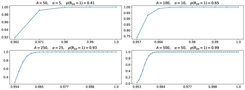
Figure 2: Probability of achieving a perfect point-adjust recall ($p(\text{R}_{pa}=1$) for four different datasets that have the same contamination rate, $r=0.1$, but different anomalous segment’s lengths. For each dataset, we randomly select $1\%$ of the points ($\alpha$) and tag them as anomalous. Each subplot represents the CDF of the corresponding $\text{F1}_{pa}$ score. That is, the x-axis represents threshold values and the y-axis is the probability of obtaining an $\text{F1}_{pa}$ score $\leq$ the corresponding threshold value. Each value corresponds to $s\in[1,\alpha]$, the number of successes hitting the anomalous segment. We can see that for the same contamination rate across datasets, we are more confident about obtaining fairly high $\text{F1}_{pa}$ scores as the length of the anomalous segment increases. For $A=500$ for example, the probability of having $\text{F1}_{pa}\leq 0.953$ is close to $0$.

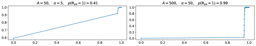
Figure 3: Probability of achieving a perfect point-adjust recall ($p(\text{R}_{pa}=1$) for $A=50$ and $A=500$. Unlike Fig. 2, this figure shows the CDF starting from $\text{F1}_{pa}=0$.

In Fig. 2 and 3, the probability of achieving a perfect point-adjust recall for $A=50$ is $0.41$ and that of having $\text{F1}_{pa}=0$ is fairly high ($0.61$). These probabilities are based on $\alpha=5$. It turns out that we can improve these scores and their probabilities by using better values for $\alpha$ while keeping other parameters unchanged (i.e., $A=50$ and $r=0.1$). Fig. 4 shows the probability of achieving a perfect point-adjust recall for different values of $\alpha$, and the worst resulting $\text{P}_{pa}$ and $\text{F1}_{pa}$ scores. These worst scores are reached if, out of $\alpha$ randomly selected points, one single point falls within the anomalous segment and $\alpha-1$ points outside of it. For $\alpha=26$, for example, $p(\text{F1}_{pa}\geq 0.8)\approx 0.935$.

In practice, using this procedure with $\alpha=1000$ yielded an average $\text{F1}_{pa}$ score of about $0.95$ for SWaT and Wadi datasets and $0.98$ for PSM. These scores are higher than the ones obtained using elaborate DL-based pipelines.

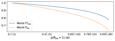
Figure 4: Probability of achieving a perfect point-adjust recall ($p(\text{R}_{pa}=1$) for $A=50$ and $r=0.1$ for different values of $\alpha$, as well the worst corresponding values of $\text{F1}_{pa}$ and $\text{P}_{pa}$. The worst values correspond to the case where one single point within the anomalous segment and $\alpha-1$ points from outside the segment are respectively tagged as anomalous. Each $x$ value corresponds to $p(\text{R}_{pa}=1)$ given a value of $\alpha$.

3.2 Point-wise: a Good Protocol but not for All Situations

This protocol consists of computing the precision, recall and F1 score based on the actual output of the algorithm, without any “adjustment”. There is nothing special about this procedure, which is used in many other fields. One interesting feature of the F1 score is that it is generally a good default choice for unbalanced datasets. An unbalanced dataset contains a dominant class with the majority of points belonging to it. However, in many cases, including anomaly detection, it is often desirable to know the number of false alarms raised by an algorithm or at least their rate, referred to as False Alarm Rate (FAR), and computed as the number of false alarms to the total number of normal points.

Consider for instance an anomaly detection algorithm used to detect upcoming hard disk failures in a data center. Detecting an upcoming failure means that the disk should be replaced. Using the FAR as one of the metrics to evaluate the algorithm helps estimate the expected number of unduly replaced disks and the resulting cost. This is not possible when using the precision or the F1 score.

To further illustrate the limits of the F1 score, we consider many anomaly detectors that have all the same recall of $0.99$, but a FAR that varies across detectors ($0.001\leq\text{FAR}\leq{0.2}$). We compute the F1 score of each of these detectors with three datasets that have the same number of normal points ($10000$) but a different number of anomalous points (5000, 1000 and 100 points respectively, meaning that the datasets have a different contamination rate). Fig. 5 shows the F1 score of each of these detectors for the three datasets. As can be observed, for a given detector (one tick on the x-axis), the F1 scores vary considerably depending on the number of anomalous points in the dataset.

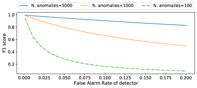
Figure 5: F1 score of many anomaly detectors on three different datasets. All detectors have the same recall of 0.99, but a different False Alarm Rate (i.e., each detector has its own FAR). Each curve corresponds to a dataset that has $10000$ normal points but a different number of anomalous points (the datasets have, therefore, a different contamination rate). We can see that, even if the recall and the FAR of a detector are the same for all datasets, its F1 score may be much higher for datasets with a high contamination rate than for datasets with a low contamination rate. This is particularly true for detectors with a high FAR.

This happens because the precision and, as a result, the F1 score, are also a function of TP: a higher TP results in a better precision and F1 score. In fact, as the FAR of a detector is the same across datasets, and as the three datasets have the same number of normal points, the expected FP is the same for the detector across datasets. However, as the number of anomalous points is not the same for all datasets, the TP of a detector is higher for datasets with more anomalies. As a result, the precision and F1 score are better for datasets with a higher contamination rate. Consequently, the precision and the F1 score can only yield a coarse estimation of false alarms and can hardly be used to accurately estimate their cost in terms of money, time, human effort, etc.

More related to time series, another case where F1 score computed in the point-wise fashion has limits is when anomalies make up lengthy segments rather than isolated outliers. We refer to these segments as anomalous events. In principle, if two algorithms have roughly the same FAR, one would prefer the one that detects more events even if its point-wise recall is lower. The point-wise F1 score does not allow algorithm comparison from that perspective, and does not let us know how many events were ever detected by an algorithm.

The limits of the point-wise F1 score may be exacerbated for benchmark datasets that contain one or a couple of very long events compared to the rest of events. In such cases, an algorithm may be tuned to efficiently detect anomalies within the lengthy events, while probably (and seamlessly) being less efficient for shorter events. This is for example the case for the SWaT dataset, in which the median event length is 450 points, but there is one 35K-point event that is, furthermore, the most anomalous and the easiest to detect.

3.3 Alternative Evaluation Protocols

3.3.1 The Composite Protocol

By design, the point-wise F1 score treats TP and FP alike (and also FN, but this point in not necessary to the current discussion). As a result, each TP is celebrated as one more detected anomaly and each FP is regarded as a false alarm. The problem is that, for benchmark datasets that contain anomalous events, the very first anomaly detected within an event is normally more informative than consecutively detected anomalies within the same event. Hence, the symmetry with which point-wise protocol considers TP and FP is no longer justified. Based on this reasoning, Garg et al. [8] propose to count just one TP for each detected event, regardless of the number of anomalous points detected within it. The recall is hence computed at the event level. However, to compute the precision, the TP and FP at the point level are used, just like with the point-wise protocol. The resulting F1 score, referred to as $\text{F1}_{C}$ in the following, is called composite. This protocol is much more appropriate than the point-wise protocol for datasets in which anomalies take the form of long events, and we believe it should be paid more attention in future works.

3.3.2 The Event-wise Protocol

Motivated by the conclusions of [8], and in an attempt to 1) partially disentangle the precision from TP and give more weight to false alarms, and 2) make the performance of algorithms easier and more intuitive to interpret, we propose the event-wise protocol.

The event-wise protocol computes TP at the event level, as in the composite protocol. However, FP is not counted at the point level, as with the point-wise and composite protocols, but is the number of anomalous segments found by the algorithm that do not overlap with any Ground Truth (GT) event. For clarity, we use “segment” to refer to any set of contiguous points that the algorithm considers anomalous, and “event” to refer to a GT anomalous event. Based on this, we define the following event-wise metrics:

• $\text{TP}_{E}$: number of GT events that fully or partially overlap with one segment or more. The event-wise recall is calculated as $\text{R}_{E}=\frac{\text{TP}_{E}}{\text{\# GT events}}$. This is the same recall used in the composite protocol.

• $\text{FN}_{E}$: number of GT events that do not overlap with any segment.

• $\text{FP}_{E}$: number of segments that do not overlap with any GT event. This includes segments of many points as well as isolated points. The event-wise precision can be computed as $\text{P}_{E}=\frac{\text{TP}_{E}}{\text{TP}_{E}+\text{FP}_{E}}$.

A similar protocol was proposed by [10] but has not been much used in consecutive works. This is likely due to one serious issue it has: an algorithm that predicts an alarm for every point (e.g., algorithm A3 in Fig. 6) would have prefect event-wise recall ($\text{R}_{E}$) and precision ($\text{P}_{E}$). To avoid this, we propose to involve the FAR at the point level in the computation of the event-wise precision. The precision at the event level is therefore computed as:

$$\text{P}_{E}=\frac{\text{TP}_{E}}{\text{TP}_{E}+\text{FP}_{E}}\times(1-\text{FAR})$$ (6)

where $\text{FAR}=\frac{\text{FP}}{N}$ and $N$ is the number of normal points in data. The event-wise F1 score, denoted $\text{F1}_{E}$, is then computed in terms of $\text{R}_{E}$ and $\text{P}_{E}$.

Fig. 6 illustrates this protocol with the outputs of three algorithms. Note that algorithm A3 has $\text{F1}_{E}=0$ even though it has a perfect event-wise recall. This is the case because this algorithm has a $\text{FAR}=1$. Thanks to the introduction of FAR in the computation of the precision, the proposed event-wise protocol is more sensitive to false alarms compared to other protocols, and is less dependent on TP or on the number of anomalous points in the dataset.

Figure 6: Illustration of the event-wise protocol with three GT events and the outputs of three algorithms. Algorithm A1 detects all events without false alarms (i.e., it has no segment that does not overlap with any event). Despite this, its precision is not perfect because its second segment is too long. Algorithm A2 achieves an event-wise recall of 2/3 and a low precision because its $\text{FP}_{E}=3$. Algorithm A3 detects all events but its event-wise precision, $\text{P}_{E}$, and its $\text{F1}_{E}$ score equal $0$ because its FAR is $1$.

4 Benchmark Datasets, Experiment Design and Algorithms Comparison

Wu and Keogh [16] discuss flaws of a few datasets for univariate and multivariate time series used for anomaly detection, and how trivial solutions can achieve state-of-the-art performance on them. In this section, we discuss other issues related to a few popular MVTS datasets and certain practices in terms of evaluation that hinder objective algorithm comparison.

SWaT and Wadi are two very popular MVTS benchmark datasets for anomaly detection. They are fairly big in terms of number of points and have each many anomalous events introduced by deliberately manipulating parts of the system from which they are collected. However, these datasets are shared by their publishers in a raw format upon subscription, with incoherent labeling for the former and two data versions for the latter.

The SWaT dataset, for example, has one integrated label column as well as a separate file that contains the start and the end of anomalous events. Using events’ start and end to reconstruct the labels does not result in the same content as in the integrated label column. Wadi has two versions from 2017 and 2019, with different sizes and different anomaly ratios. This situation has led to a disagreement about the characteristics of these datasets across papers.

Furthermore, as mentioned earlier, the SWaT dataset contains one anomalous event that is much longer than other events. This event contributes to the F1 score much more than other events and explains the relatively high scores of many algorithms using the point-wise protocol with this dataset compared to other datasets. Actually, by shortening this event to the median event length, [8] showed a significant drop in the point-wise F1 score for all algorithms. While this is an interesting finding, we do not advocate for deliberate event shrinking because it may introduce artifacts and subtle changes in the data, making the event easier to detect. We believe that this issue can be better dealt with using event-aware evaluation protocols like the ones introduced in section 3.3

The use of different evaluation protocols across publications has also led to situations where authors evaluate their algorithm with the point-adjust protocol but report results of other approaches using the point-wise protocol. This is for example observed in [6], which evaluates the proposed algorithm using point-adjust and compares the results to at least one algorithm (GDN [7]) using the point-wise protocol. Other works, such as [15], use the point-adjust protocol without even mentioning it in the text. These practices, which may be observed in other works (and which we assume are not intentional), are very likely to be misleading for uninformed readers, including reviewers. Finally, in [13] the authors explicitly confirm that they do not use the point-adjust protocol, citing what is probably the main work highlighting the flaws of this protocol as of today, [11]. However, reported scores for the proposed algorithm, as well as for state-of-the-art algorithms considered for comparison, look as high as the usual point-adjust scores encountered in many studies with the same datasets.

5 Algorithms

In this part, we evaluate three DL-based algorithms for MVTS anomaly detection, as well as a baseline algorithm based on PCA. These DL-based approaches are selected because they are quite recent, introduce very interesting ideas, and achieve a high performance with the used protocols. Moreover, all of these approaches have an official open-source implementation that we used in our experiments. The approaches are:

• Anomaly Transformer [17], uses Transformers to model time series dynamic patterns. Evaluated using the point-adjust protocol only in original work.

• NCAD [4], uses a 1D Convolutional Neural Network (CNN) to obtain feature representations of data. Also evaluated using the point-adjust protocol only in original work.

• GDN [7], uses GNNs to learn the relationship between time series to achieve a better forecasting performance. Evaluated using the point-wise protocol only in original work.

Our goal is to challenge these algorithms with different evaluation protocols and confront them with PCA. Table 1 summarizes the obtained results with point-wise, composite and event-wise protocols. It also reports the number of detected events ($\text{TP}_{E}$) and the number of predicted anomalous segments that do not overlap with any GT event ($\text{FP}_{E}$, see Fig. 6). Results are obtained using the SWaT (with labels constructed from attacks’ start and end), Wadi (2017 version), and PSM datasets.

	SWaT				Wadi				PSM
	F1	$\text{F1}_{C}$	$\text{F1}_{E}$	$\text{TP}_{E}$/$\text{FP}_{E}$	F1	$\text{F1}_{C}$	$\text{F1}_{E}$	$\text{TP}_{E}$/$\text{FP}_{E}$	F1	$\text{F1}_{C}$	$\text{F1}_{E}$	$\text{TP}_{E}$/$\text{FP}_{E}$
AT	0.214	0.214	0.000	35/0	0.108	0.108	0.000	14/0	0.434	0.434	0.000	72/0
NCAD	0.217	0.217	0.002	35/694	0.114	0.115	0.003	14/1394	0.429	0.429	0.000	72/0
GDN	0.821	0.488	0.478	11/0	0.567	0.764	0.485	9/14	0.594	0.640	0.096	63/843
PCA	0.810	0.596	0.555	15/4	0.374	0.655	0.608	7/2	0.538	0.484	0.200	32/170

Table 1: Comparative results of AnomalyTransformer (AT), NCAD, GDN and PCA using the point-wise (F1), composite ($\text{F1}_{C}$) and event-wise ($\text{F1}_{E}$) protocols. All metrics are computed based on the detection threshold that yields the best point-wise performance. The SWaT, Wadi and PSM datasets have 35, 14 and 72 events and a contamination rate of $11.98\%$, $5.71\%$ and $27.76\%$ respectively.

These results reveal several interesting findings, summarized as follows:

• Algorithms that were developed using point-adjust as the sole target fail to reach any score better than a random guess when evaluated with other protocols. This is the case of AnomalyTransformer and NCAD. For completeness, we also evaluated these algorithms using the point-adjust protocol and achieved the same, very high, scores reported in the original papers. It is worth mentioning that we also achieved essentially the same high scores using untrained versions of these models. We assume that many other approaches developed using the same setting would face the same problem.

• GDN, however, which was developed based on the more realistic point-wise protocol, shows more resilience when evaluated with other protocols.

• Datasets that have a very high contamination rate, such as PSM, yield point-wise F1 scores that can be misleading. AnomalyTransformer and NCAD, for example, achieve a point-wise F1 score around $0.43$, which may look as a fairly good baseline score. In fact, based on the contamination rate of the dataset, this score is achievable by predicting all or most points as anomalous, and this is what these algorithms are doing. The composite score is comparable to the point-wise score in this case and does not bring any useful information. The event-wise score, however, severely penalizes such approaches thanks to the inclusion of FAR in score computation.

• Finally, we show that PCA, which is not considered as a particularly advanced approach for MVTS anomaly detection, achieves an honorable point-wise score compared to many recent DL-based approaches (e.g., USAD [3], MSCRED [18], OmniAnomaly [14] and DAGMM [20], see [11] for a summary of the performance of these approaches). Our conclusion here is that many works have been developed without establishing a simple but enough challenging baseline. Actually, the bar of $0.8$ point-wise F1 score for the SWaT dataset had been a symbolic target for many years until recent GNN-based approaches, such GDN [7] and FuSAGNet [9], reached it. In our PCA-based pipeline, we use simple pre-processing and post-processing blocks (input scaling, clipping and score smoothing) that significantly improve the score.

Scores in Table 1 are obtained using the threshold that yields the best point-wise F1 score. To further understand the decisions of algorithms such as AnomalyTransformer and NCAD, we used the threshold that yields the best point-adjust score for these algorithms and looked at their outputs to better understand their behavior. As aforementioned, using the point-adjust protocol, we obtained scores comparable to those reported in original papers for these algorithms (actually, we achieved even higher scores). The first row in Fig. 7 shows all GT events of SWaT as well as the outputs of AnomalyTransformer that lead to a $0.97$ $\text{F1}_{pa}$ score. By zooming in on smaller parts of the dataset (the three first events, then just the first one), we see that the algorithm predicts anomalies at an almost regular pace. More precisely, using the threshold that ensures the best $\text{F1}_{pa}$ score results in a total of 4097 points predicted as anomalous, of which 473 lie within an anomalous event and 3624 outside any anomalous event. Knowing that the whole test dataset is about 5 days long, has one point per second, and a total of 35 anomalous events, the algorithm, with such an output, helps detect all 35 events while raising 3624 false alarms over 5 days. On average, it raises an alarm every 110 seconds, making it, in our opinion, barely useful for deployment. Such a behavior is generously rewarded by the point-adjust protocol.

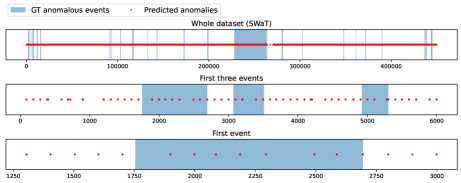
Figure 7: Ground Truth anomalous events of the SWaT dataset and outputs of AnomalyTransformer. The second and third rows zoom in on the first three events and on the first event, respectively. We can see that all the algorithm is doing is output an anomaly prediction at almost regular intervals. This ensures a $0.97$ $\text{F1}_{pa}$ score. Note that on the first row (whole dataset), there are exactly 4097 red dots ($\leq 1\%$ of the total points) but they look many more because the size of the dots is intentionally big for visualization purposes.

6 Discussion: Towards Better Practices for MVTS Anomaly Detection

6.1 Evaluation Protocols and Metrics

The point-adjust protocol has had its very illegitimate hour of glory and created what Wu and Keogh [16] call “illusion of progress” in probably quite a unique way in machine learning. We believe that this protocol should no longer be used. Authors should resist the temptation of publishing high but misleading scores using it, and reviewers should be aware of its flaws and advise authors to report results using other protocols.

Evaluating algorithms for time series anomaly detection is not a trivial task. The point-wise protocol may be good as a straightforward way to compare and rank algorithms, but other protocols and metrics, especially event-aware ones, should be used alongside this protocol when possible. For datasets that contain anomalous events/episodes, at least the number of detected events should be reported for each algorithm alongside point-wise metrics.

6.2 Datasets and Experiment Design

By sharing the raw versions of SWaT and Wadi datasets, the publishers apparently wanted to give researchers the freedom to experiment with the data the way they want. However, this has led to a divergence in the way these datasets are described and used in the literature. We believe that it would be better that the data be stored in a unique, accessible place using a format that anyone can start experimenting with quickly. Ideally, part of the test data would be provided without labels so that researchers upload the output of their algorithms to a third-party server for evaluation and publication on a public leaderboard.

6.3 Algorithms

As mentioned in section 1, recent approaches for MVTS anomaly detection have been marked by quite a few innovative ideas. However, based on the methodology issues discussed in this paper, our position on this is the following: while many of the proposed approaches are conceptually very appealing, we believe that the merits of most of them are yet to be confirmed in the light of more appropriate evaluation protocols.

Researchers should find a balance between the effort allocated to designing efficient algorithms and that allocated to running sound experiments. Based on our experiments and on the results shown by [11] using an untrained model, it is reasonable to assume that studies using the point-adjust protocol achieved high scores in a relatively short time. Oftentimes in machine learning, an abnormally high score is achieved with little effort either because the problem at hand is trivial, due to a data leakage somewhere in the pipeline, or due to a bug in evaluation code. Admittedly, when the main cause is a widely used evaluation protocol, it can be much harder to uncover, hence the need to discuss evaluation protocols and their potential weaknesses and biases.

References

- [1] Abdulaal, A., Liu, Z., Lancewicki, T.: Practical approach to asynchronous multivariate time series anomaly detection and localization. In: Proceedings of the 27th ACM SIGKDD Conference on Knowledge Discovery & Data Mining. pp. 2485–2494 (2021)
- [2] Ahmed, C.M., Palleti, V.R., Mathur, A.P.: Wadi: a water distribution testbed for research in the design of secure cyber physical systems. In: Proceedings of the 3rd international workshop on cyber-physical systems for smart water networks. pp. 25–28 (2017)
- [3] Audibert, J., Michiardi, P., Guyard, F., Marti, S., Zuluaga, M.A.: Usad: Unsupervised anomaly detection on multivariate time series. In: Proceedings of the 26th ACM SIGKDD International Conference on Knowledge Discovery & Data Mining. pp. 3395–3404 (2020)
- [4] Carmona, C.U., Aubet, F.X., Flunkert, V., Gasthaus, J.: Neural contextual anomaly detection for time series. Proceedings of the Thirty-First International Joint Conference on Artificial Intelligence, IJCAI-22 (2022)
- [5] Chen, X., Deng, L., Huang, F., Zhang, C., Zhang, Z., Zhao, Y., Zheng, K.: Daemon: Unsupervised anomaly detection and interpretation for multivariate time series. In: 2021 IEEE 37th International Conference on Data Engineering (ICDE). pp. 2225–2230. IEEE (2021)
- [6] Chen, Z., Chen, D., Zhang, X., Yuan, Z., Cheng, X.: Learning graph structures with transformer for multivariate time series anomaly detection in iot. IEEE Internet of Things Journal (2021)
- [7] Deng, A., Hooi, B.: Graph neural network-based anomaly detection in multivariate time series. In: Proceedings of the AAAI Conference on Artificial Intelligence. vol. 35, pp. 4027–4035 (2021)
- [8] Garg, A., Zhang, W., Samaran, J., Savitha, R., Foo, C.S.: An evaluation of anomaly detection and diagnosis in multivariate time series. IEEE Transactions on Neural Networks and Learning Systems 33(6), 2508–2517 (2021)
- [9] Han, S., Woo, S.S.: Learning sparse latent graph representations for anomaly detection in multivariate time series. In: Proceedings of the 28th ACM SIGKDD Conference on Knowledge Discovery and Data Mining. pp. 2977–2986 (2022)
- [10] Hundman, K., Constantinou, V., Laporte, C., Colwell, I., Soderstrom, T.: Detecting spacecraft anomalies using lstms and nonparametric dynamic thresholding. In: Proceedings of the 24th ACM SIGKDD international conference on knowledge discovery & data mining. pp. 387–395 (2018)
- [11] Kim, S., Choi, K., Choi, H.S., Lee, B., Yoon, S.: Towards a rigorous evaluation of time-series anomaly detection. In: Proceedings of the AAAI Conference on Artificial Intelligence. pp. 7194–7201 (2022)
- [12] Mathur, A.P., Tippenhauer, N.O.: Swat: A water treatment testbed for research and training on ics security. In: 2016 international workshop on cyber-physical systems for smart water networks (CySWater). pp. 31–36. IEEE (2016)
- [13] Pan, J., Ji, W., Zhong, B., Wang, P., Wang, X., Chen, J.: Duma: Dual mask for multivariate time series anomaly detection. IEEE Sensors Journal (2022)
- [14] Su, Y., Zhao, Y., Niu, C., Liu, R., Sun, W., Pei, D.: Robust anomaly detection for multivariate time series through stochastic recurrent neural network. In: Proceedings of the 25th ACM SIGKDD international conference on knowledge discovery & data mining. pp. 2828–2837 (2019)
- [15] Tuli, S., Casale, G., Jennings, N.R.: TranAD: Deep Transformer Networks for Anomaly Detection in Multivariate Time Series Data. Proceedings of VLDB 15(6), 1201–1214 (2022)
- [16] Wu, R., Keogh, E.: Current time series anomaly detection benchmarks are flawed and are creating the illusion of progress. IEEE Transactions on Knowledge and Data Engineering (2021)
- [17] Xu, J., Wu, H., Wang, J., Long, M.: Anomaly transformer: Time series anomaly detection with association discrepancy. The Tenth International Conference on Learning Representations (2022)
- [18] Zhang, C., Song, D., Chen, Y., Feng, X., Lumezanu, C., Cheng, W., Ni, J., Zong, B., Chen, H., Chawla, N.V.: A deep neural network for unsupervised anomaly detection and diagnosis in multivariate time series data. In: Proceedings of the AAAI conference on artificial intelligence. vol. 33, pp. 1409–1416 (2019)
- [19] Zhang, W., Zhang, C., Tsung, F.: Grelen: Multivariate time series anomaly detection from the perspective of graph relational learning. In: Proceedings of the Thirty-First International Joint Conference on Artificial Intelligence (IJCAI) (2022)
- [20] Zong, B., Song, Q., Min, M.R., Cheng, W., Lumezanu, C., Cho, D., Chen, H.: Deep autoencoding gaussian mixture model for unsupervised anomaly detection. In: International conference on learning representations (2018)