Data-Side Efficiencies for Lightweight Convolutional Neural Networks

Abstract

We examine how the choice of data-side attributes for two important visual tasks of image classification and object detection can aid in the choice or design of lightweight convolutional neural networks. We show by experimentation how four data attributes – number of classes, object color, image resolution, and object scale affect neural network model size and efficiency. Intra- and inter-class similarity metrics, based on metric learning, are defined to guide the evaluation of these attributes toward achieving lightweight models. Evaluations made using these metrics are shown to require $30\times$ less computation than running full inference tests. We provide, as an example, applying the metrics and methods to choose a lightweight model for a robot path planning application and achieve computation reduction of $66\%$ and accuracy gain of $3.5\%$ over the pre-method model.

Keywords Efficient Neural Network  $\cdot$ Convolutional Neural Network  $\cdot$ Image Classification  $\cdot$ Object Detection

1 Introduction

Traditionally for computer vision applications, an algorithm designer with domain expertise would begin by identifying handcrafted features to help recognize objects of interest. More recently, end-to-end learning (E2E) has supplanted that expert by training a deep neural network to learn important features on its own. Besides the little forethought required about data features, there is usually only basic preprocessing done on the input data; an image is often downsampled and converted to a vector, and an audio signal is often transformed to a spectogram. In this paper, we use the term “data-side” to include operations that are performed on the data before input to the neural network. Our proposal is that a one-time analysis of data-side attributes can aid the design of more efficient convolutional neural networks (CNNs) for the many-times that they are used to perform inferences.

On the data side of the neural network, we examine four independent image attributes and two dependent attributes, the latter which we use as metrics. The independent attributes are number of classes, object color, image resolution and object scale. The metrics are intra- and inter-class similarity. Our goal is to optimize the metrics by choice of the independent variables – specifically to maximize intra-class similarity and minimize inter-class similarity – to obtain the most computationally efficient model.

Unlike benchmark competitions such as ImageNet [1], practical applications involve a design stage that can include adjustment of input specifications. In Section 2, we tabulate a selection of applications. The “wildlife” application reduced the number of animal and bird classes from 18 to 6 in the Wildlife Spotter dataset [2]. In the “driving” application [3], the 10 classes of the BDD dataset [4] were reduced to 7 by eliminating the “train” class due to few labeled instances and combining the similar classes of rider, motor, and bike into rider.

The main contributions of this paper are:

1. Four data-side attributes are identified, and experiments are run to show their effects on the computational efficiency of lightweight CNNs.

2. Intra- and inter-class similarity metrics are defined to aid evaluation of the four independent attribute values. Use of these metrics is shown to be about $30\times$ faster than evaluation by full inference testing.

3. Procedures are described using the similarity metrics to evaluate how changing attribute values can reduce model computation while maintaining accuracy.

4. Starting with the EfficientNet-B0 model, we show how our methods can guide the application designer to smaller “sub-EfficientNets” with greater efficiency and similar or higher accuracy.

We describe related work in Section 2. Each of the attributes is defined in Section 3, procedures are described to apply these toward more efficient models in Section 4, and experimental evidence is shown in Section 5. We conclude in Section 6.

2 Related Work

The post-AlexNet [5] era (2012-) of convolutional neural networks brought larger and larger networks with the understanding that a larger model yielded higher accuracy (e.g., VGGNet-16 [6] in 2014 with 144M parameters). But the need for more efficiency, especially for embedded systems [7], encouraged the design of lightweight neural networks [8], such as SqueezeNet [9] in 2017 with 1.2M parameters. Models were reduced in size by such architectures as depthwise separable convolution filters  [10]. More efficient handling of data was incorporated by using quantization  [11, 12, 13], pruning  [14, 15, 16, 17], and data saliency [18]. This model-side efficiency quest is a common research trend where new models are evaluated for general purpose classification and object detection on public benchmarks such as ImageNet  [1], COCO  [19], and VOC  [20]. Orthogonal and complementary to these model-side efficiencies  [21, 22, 23], we examine efficiencies that can be gained before the model by understanding and adjusting the data attributes within the confines of the application specifications. Early work  [24] optimizes models specialized to the target video only for binary-classification. Our work extends to multi-class classification and object detection.

In Table 1, we list a selection of 9 applications whose data attributes are far less complex than common benchmarks. For these applications, class number is often just 2. The largest number of classes, 7, is for the “driving” [4] application. Compare these with 80 classes for the COCO dataset and 1000 for ImageNet. For 2 applications, color is not used. For the “crowd” application, it is not deemed useful and for the “ship, SAR” application, the input data is inherently not color. The resolution range is not broad in this sampling, likely due to matching image size to model input width. Many papers did not describe the scale range; for these, we approximated from the given information or images in the paper. The broadest scale range (as a fraction of image size) is the “driving” application ($1/32$ to $1/2$), and the narrowest is for the “mammals” application, using aerial image capture, with scale from $1/30$ to $1/20$.

Application	$N_{Cl}$	$N_{Co}$	$R_{E}$	$S_{C}$
crowd [25]	2	no	$320\times 240$	$1/8$, $1/2$
ship, SAR [26]	2	no	$416\times 416$	$1/20$, $1/6$
cattle [27]	2	yes	$224\times 224$	$1/16$, $1/2$
hardhat [28]	2	yes	$300\times 300$	$1/25$, $1/2$
wildlife [2]	6	yes	$224\times 224$	$1/6$, $1/2$
PCB defect [29]	6	yes	$640\times 640$	$1/30$, $1/15$
ship [30]	6	yes	$416\times 416$	$1/20$, $1/2$
mammals [31]	6	yes	2k $\times$ 2k	$1/30$, $1/20$
driving [3]	7	yes	608 $\times$ 608	$1/32$, $1/2$

Table 1: Examples of data attributes for object detection applications with attributes: number of classes ($N_{Cl}$), color ($N_{Co}$), input resolution ($R_{E}$), and scale range ($S_{C}$) as a fraction of image size.

We use a measure of class similarity to efficiently examine data attributes, based on neural network metric learning. This term describes the use of learned, low-dimensional representations of discrete variables (images in our case). The distance between two instances in the latent space can be measured by L1  [32], L2, or cosine similarity  [33]. Previous studies  [34, 35, 36] focus on learning a single similarity latent space. Differences between classification  [37] and ranking based losses  [38] have been studied in  [39]. PAN incorporates attributes to visual similarity learning  [40]. In Sections 3.6 and 3.7 we extend this line of research by adapting the metric from  [33] to measure intra- and inter-class similarity to serve efficiency purposes.

In contrast to research to improve model performance on public benchmarks, our goal is to develop an empirical understanding of the effects of these attributes on common CNNs, and from this to provide practical guidelines to obtain lightweight CNNs in real-world scenarios. Our use of intra- and inter-class similarity metrics enables an efficient methodology toward this goal. Practical, low-complexity applications as in Table 1 can benefit from our investigation and method.

3 Data Attributes and Metrics

This work is centered on the hypothesis that, the easier the input data is to classify, the more computationally efficient the model can be at a fixed or chosen lower accuracy threshold. In this section, we describe each of the data attributes and their relationships to the hypothesis. We define metrics to obtain the dependent variables. And we describe procedures to adjust the independent variables to obtain metrics that guide the design of an efficient model.

We first introduce the term, Ease of Classification $EoC$ and hypothesize the following relationship exists with the data-side attributes,

$$\mathrm{EoC}\leftarrow({S_{1}},\frac{1}{S_{2}})\leftarrow(\frac{1}{N_{Cl}},\frac{1}{N_{Co}},\frac{1}{R_{E}},\frac{1}{S_{C}}).$$ (1)

The symbol ($\leftarrow$) is used to describe the direct relationships in which the left expressions are related to the right. $EoC$ increases with intra-class similarity $S_{1}$ and decreases with inter-class similarity $S_{2}$. The dependent variable $S_{1}$ is related to the reciprocals of the independent variables, number of classes $N_{Cl}$, number of color channels $N_{Co}$, image resolution $R_{E}$, and object scale $S_{C}$. The dependent variable $S_{2}$ is directly related to these independent variables. The model designer follows an approach to adjust these independent variables to obtain similarity measurements that achieve high $EoC$. Note that we will sometimes simplify $N_{Cl}$ to $CL$ for readability in figures.

In Section 5 we perform experiments on a range of values for each attribute to understand how they affect model size and accuracy. However, these experiments cannot be done independently for each attribute because some have dependencies on others. We call these interdependencies because they are 2-way. We discuss interdependencies below for two groups, {$S_{C}$, $R_{E}$} and {$S_{1}$, $S_{2}$, $N_{Cl}$}.

3.1 Number of Classes, $N_{Cl}$

The $N_{Cl}$ attribute is the number of classes being classified in the dataset. Experimental results with different numbers of classes are shown in Section 5.2. In Section 5.6 we present results of changing the number of classes for a robot path planning application.

3.2 Object Colors, $N_{Co}$

The $N_{Co}$ attribute is the number of color axes, either 1 for grayscale or 3 for tristimulus color models such as RGB (red, green, blue). When the data has a color format, the first layer of the neural model has 3 channels. For grayscale data input, the model has 1 input channel. In Section 5.3, we show the efficiency gain for 1 versus 3 input channels.

3.3 Image Resolution, $R_{E}$

Image resolution, measured in pixels, has the most direct relationship to model size and computation. Increasing the image size by a multiple $m$ (rows $I_{r}$ to $m\times I_{r}/2$ and columns $I_{c}$ to $m\times I_{c}$) increases the computation by at least one-to-one. In Figure 1, MobileNet computation increases proportionally to image size. The lower sized EfficientNet-B0 and -B1 models also increase proportionally, but rise faster with larger models B2, B3, and B4.

It is not the case that higher resolution always yields better accuracy. It usually plateaus, and that plateau is different for different classes involved. The objective is to choose the minimum image resolution before which accuracy drops unacceptably. Note that resolution and scale are dependent attributes, and neither can be adjusted without considering the effect on the other. Experimental results with different resolutions are shown in Section 5.5.

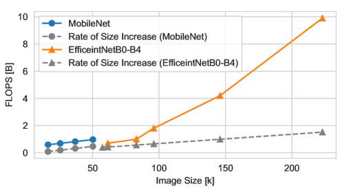
Figure 1: As the input image size is increased, the computation for the smaller MobileNet models increase at a similar rate. For the larger EfficientNet models (only up to EfficientNet-B4 are shown for clarity of display), the computation increases at a higher rate.

3.4 Object Scale, $S_{C}$

For a CNN, the image area, or receptive field, of a $3\times 3$ filter kernel expands as the following sequence for layers $L=1,2,3,...,L$,

$$3\times 3,7\times 7,15\times 15,\ldots,(2^{L+1}-1)\times(2^{L+1}-1).$$ (2)

For object detection, this means that, if the maximum object size in an image is, for example, $15\times 15$, the network needs at least 3 layers to yield features that convolve with (or overlap) the full size of these objects. In practice, from the sequence in equation 2 the minimum number of layers can be found from the maximum sidelength $b_{max}$ of bounding boxes of objects over all image instances,

$$L\geq\lceil\mathrm{log}_{2}(b_{max}+1)\rceil-1.$$ (3)

where $\lceil x\rceil$ is a ceiling operator, which rounds the $x$ value to the higher integer. For example, if $b_{max}$ is 250, the minimum number of layers needed is $\lceil 7.966\rceil-1=7$.

In practice, the maximum object size is approximated as the longer sidelength of the bounding box of the object. In terms of model size and minimizing computation, by measuring the bounding box size of objects in a dataset, one can discover the maximum number of layers needed for full-object feature extraction. Furthermore, using filter kernels that are larger than the maximum object size increases extractions of inter-object features. When generalized to a sequence of rectangular filters, these tend toward Gaussian filters with increasing convolution layers, so the filter edge versus middle magnitude lowers as well.

To decouple scale from resolution, we define the scale of an object as a fraction of the longer image dimension. With this definition, one can measure the scale of an object in an image without knowing the resolution. The size of the object is measured in pixels; it is the product of scale times the longer dimension of the resolution. Figure 2 shows the range of scales for objects in the COCO datase. Although 50% of instances account for $\leq 10\%$ of image size, still the sizes range from very small to full image size. Conversely, in many applications, scale range is known and much more contained as for some applications in Table 1. Experimental results with different scales are shown in Section 5.5.

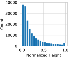
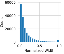
Figure 2: Histogram of bounding box sizes in COCO training dataset highly skewed at small sizes $<0.2$.

3.5 Resolution and Scale Interdependency

The interdependence between the attributes {$S_{C}$, $R_{E}$ } is common to any image processing application, and can be described by two cases. For case 1, if the scale of objects within a class in an image is large enough to reduce the image size and still recognize the objects with high accuracy, then there is a resulting benefit of lower computation. However, reducing the image size also reduces resolution, and if there is another class that depends upon a high spatial frequency feature such as texture, then reducing the image would reduce overall accuracy. For case 2, if resolution of the highest frequency features of a class is more than adequate to support image reduction, then computational efficiency can be gained by reducing the image size. However, because that reduction also reduces scale, classes that are differentiated by scale will become more similar, and this situation may cause lower accuracy. We can write these relationships as follows,

$$(S_{C}\>\propto\>R_{E})\>\rightarrow\>\frac{1}{\mathrm{EoC}},$$ (4)

where the expression within parentheses is commutative (a change in $S_{C}$ will cause a proportional change in $R_{E}$, and vice versa), and these are inversely related to $EoC$.

3.6 Intra-Class Similarity, $S_{1}$

Intra-class similarity is a measure of visual similarity between members of the same class as measured with vectors in the embedding space of a deep neural network. It is described by the average and variance of pairwise similarities of instances in the class,

$$S_{1}(C_{1})=\frac{1}{N}\sum_{i,j\in C_{1}}\cos(\textbf{Z}_{i}\textbf{Z}_{j}),$$ (5)

$$\sigma_{S1}^{2}(C_{1})=\frac{1}{N}\sum_{i,j\in C_{1}}(S_{ij}-S_{1})^{2},$$ (6)

where $C_{1}$ is a class containing a set of instances, $i$ and $j$ are indices in set $C_{1}$, $i\neq j$, and $N$ is the total number of similarity pairs $S_{ij}$ of two different instances in the class. Z is the latent vector in the embedding space from a neural network trained by metric learning on instances of the class as well as other classes. (That is, it is the same model trained on the same instances as for inter-class similarity.) This metric is adapted from  [33]. We show the use of $S_{1}$ and $\sigma_{S1}^{2}$ in Section 4.1.

3.7 Inter-Class Similarity, $S_{2}$

Inter-class similarity is a measure of visual similarity between classes as determined by the closeness of instances of two classes in the embedding space of a deep neural network. For 2 classes, it is defined as the average of pairwise similarities of instances between classes,

$$S_{2}(C_{1},C_{2})=\frac{1}{N}\sum_{i\in C_{1},j\in C_{2}}\cos(\textbf{Z}_{i}\textbf{Z}_{j}),$$ (7)

where $C_{1}$ and $C_{2}$ are instance sets of two different classes, $i$ and $j$ are indices in sets $C_{1}$ and $C_{2}$ respectively, $N$ is the total number of pairs of two instances in two different classes, and Z is the latent vector in the embedding space from a neural network trained by metric learning on instances that include both classes as well as other classes if there are more than 2.

For an application involving more than two classes, we choose the inter-class similarity measure to be the maximum of inter-class similarity measures over all class pairs,

$$\hat{S_{2}}(\{C_{K}\})=\max\{S_{2}(C_{m},C_{n})\},$$ (8)

where $\{C_{K}\}$ is the set of all classes for $0<=k<K$, and $\{(C_{m},C_{n})\}$ is all class pairs for $0<=m,n<K$, $m\neq n$. We choose the maximum of similarity results of class pairs because maximum similarity represents the worst case – most difficult to distinguish – between two classes. Alternatively, one could calculate the average of inter-class similarities for each pair, however the operation of averaging will hide the effect of one pair of very similar classes among other dissimilar classes, and this effect is worse for larger $N_{Cl}$. We show the use of $\hat{S_{2}}$ in Section 4.2.

We also use a measure that is the normalized difference between the maximum and the average,

$$\Delta{S_{2}}(\{C_{K}\})=\frac{\hat{S_{2}}-S_{2}}{S_{2}}.$$ (9)

A larger $\Delta{S_{2}}$ indicates a higher value of worst case $\hat{S_{2}}$, so we seek low $\Delta{S_{2}}$ in the methods described in Sections 4.1 and 4.3.

3.8 Intra- and Inter-Class Interdependency

There is a strong interdependence between $S_{1}$ and $S_{2}$ with a secondary dependence upon $N_{Cl}$, as we will describe. With other factors fixed, smaller intra-class similarity increases inter-class similarity because more heterogeneous classes with wider attribute ranges are being compared, thus reducing $EoC$. As $N_{Cl}$ is increased, this effect is exacerbated because there is higher probability of low $S_{1}$ and high $S_{2}$ pairs, and (similarly) because we use worst-case maximum in equation 8. We can write these dependent relationships as follows,

$$(S_{1}\propto 1/S_{2})\>\rightarrow\mathrm{EoC}\>,\>\mathrm{for}N_{Cl}\geq 2,$$ (10)

where the expression within brackets is commutative (either $S_{1}$ or $S_{2}$ can cause inverse change in the other, and the relationship becomes stronger as $N_{Cl}$ increases.

4 Method

The general approach toward finding the most efficient model is to select ranges of the independent attribute values {$N_{Cl}$, $N_{Co}$, $R_{E}$, $S_{C}$}, calculate the similarity measures {$S_{1}$, $S_{2}$} for selected values in the range, and choose those independent attribute values that minimize $S_{2}$ and maximize $S_{1}$. Step-by-step procedures for selecting each of the independent attributes are described below. These procedures should be followed in the order of the sections below.

4.1 Selection of $N_{Cl}$

If the application permits adjustment of the number of classes, then the following procedure can help finding class groupings and an associated $N_{Cl}$ that supports a more efficient model. Initialize $\Delta{S_{2}}=\infty$, and follow these steps,

1. Choose class groupings.

2. Calculate $\Delta{S_{2}}$ from equation 9. If this is less than the current smallest $\Delta{S_{2}}$ then this grouping is the most efficient so far.

3. If $\Delta{S_{2}}$ is low, one can choose to exit, or continue.

4. If one decides to continue, calculate $S_{1}$ from equation 5 and $\sigma_{S1}^{2}$ from equation 6 for each class. The value of $S_{1}$ is for guidance to help understand why the current $S_{2}$ is good or bad (low or high) to give guidance on choosing the next groupings. In general, class grouping with high $S_{1}$ and low $\sigma_{S1}^{2}$ will yield higher accuracy. Repeat these steps.

We want to stop when inter-class similarity is low, indicated by a low value of $\Delta{S_{2}}$. However there is subjectivity in this step due to the manual choice of groupings and because different applications will have different levels of intra-class homogeneity and inter-class distinguishability. In practice, the procedure is usually run for a few iterations to understand relative $\Delta{S_{2}}$ values for different groupings, and the lowest is chosen.

4.2 Selection of $N_{Co}$

The application can gain computational advantage if all classes can be reduced to grayscale; if all classes cannot be reduced, then the model must handle color and there is no computational advantage. Following are the steps to choose grayscale or color,

1. For all classes in color and grayscale, calculate $\hat{S_{2}}$.

2. If $\hat{S_{2}}$ for grayscale is less than or equal to $\hat{S_{2}}$ for color, choose a grayscale model and grayscale for all instances of all classes.

If the procedure above does not result in the choice of grayscale, there is a second option. This requires more testing and does not directly yield computation reduction, but may improve accuracy.

1. For each class, calculate $\hat{S_{2}}$ against every other class for these four combinations of the $(C_{1},C_{2})$ pairs: (grayscale, grayscale), (grayscale, color), (color, grayscale), and (color, color).

2. For each class $C_{1}$ whose $\hat{S_{2}}$ for (grayscale, grayscale) and (grayscale, color) is smaller than for (color, grayscale) and (color, color), choose to use grayscale for the $C_{1}$ class.

4.3 Selection of $R_{E}$ and $S_{C}$

We first adjust the attribute $R_{E}$ to find the lower bound of resolution with respect to acceptable accuracy. Initialize $\Delta{S_{2}}=\infty$, and follow these steps,

1. Calculate $\Delta{S_{2}}$ from equation 9. If this is less than the current smallest $\Delta{S_{2}}$ then this resolution is the most efficient so far.

2. If $\Delta{S_{2}}$ is low, one can choose to exit, or continue.

3. Reduce the resolution by half and repeat these steps.

In practice, a few iterations is run to see when $\Delta{S_{2}}$ rises, then choose the resolution where it is lowest.

After the resolution has been chosen, maximum object scale is multiplied by resolution to find the maximum object size in pixels. Equation 3 is used to find an estimate of the lower bound of number of layers needed in the model.

5 Experiments

In this section, we perform experiments on the data attributes to show how their values relate to model efficiency and accuracy. Note that our level of experimentation is not even across all attributes. We believe that the experiments upon number of classes, intra- and inter-class similarities, and resolution are sufficient to support the Ease of Classification relationship of equation 1. For color, we give a quantitative comparison of color versus grayscale computation, and then because the difference is small, leave further investigation of accuracy and efficiency to cited literature. For scale, one aspect of this attribute is covered by its interdependency in the resolution experiments. However another aspect, the relationship of scale to model levels (equation 2), we leave to future work. This is because scale is less easily separated from particular applications – specifically the size range of objects in an application – than for other attributes. Our plan is to investigate this in a more application-oriented paper in the future.

5.1 Similarity Metric Efficiency

We could discover the effects of data attributes by training and inference testing all combinations of attribute values. For $N_{CL}$ classes, binary classification of pairs would require $N_{CL}\choose 2$ training and inference operations. In comparison, for similarity metrics, we need to train once for all combinations of binary classifications. During testing, the similarity model (SM) caches the latent space, thus only indices of each instance need to be paired with other instances to obtain their cosine similarities.

For the CIFAR10 dataset for example, there is a one-time task of feeding all test images into SM, which takes 0.72 seconds, and then caching, which takes 0.63 seconds. In contrast, we feed each image into the CNN to obtain its prediction in order to calculate its accuracy in the conventional pipeline. We show the runtime in Table  2 .

Model	$t_{train}$ (s/epoch)	$t_{test}$ (s/pair)
VGG19	0.69	4.49
EfficientNet-B0	3.13	21.82
MobileNetV2	2.19	15.05
Similarity Metrics	3.31	0.76

Table 2: Results of runtime comparison of Similarity Metrics and existing models. s: second, pair: all pair of instances in two classes.

5.2 Number of Classes, $N_{Cl}$

It is well known that accuracy is reduced when more classes are involved since more visual features are needed for a CNN to learn in the feature extractor backbone, as well as more complex decision boundary to learn in the fully connected layers for classification. However, we perform experiments here, first to confirm this relationship with test data, but secondly to gain any extra insight into the relationship between number of classes and accuracy.

We performed three sets of experiments. The first was for object detection using the YOLOv5-nano  [22] backbone upon increasing-size class groupings of the COCO dataset  [19]. Ten groups with $Cl$ of $\{1,2,3,4,5,10,20,40,60,80\}$ were prepared. For each group, we trained a separate YOLOv5-nano model from scratch. As seen in Figure 3 (left), accuracy decreases with number of classes. An added insight is that the accuracy decrease is steep for very few classes, say 5-10 or fewer, and flattens beyond 10.

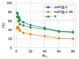
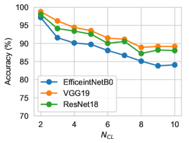
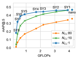
Figure 3: Overall relationship of performance and $N_{CL}$. (Left) Object detection accuracy and recall (R) decrease for the YOLOv5-nano when the number of classes is increased from 1 to 80. (Middle) CIFAR-10 Image classification accuracy decreases for the classifiers tested when the number of classes per group is increased from 2 to 10. (Right) Accuracy plot for increasingly smaller models from YOLOv5-nano through 8 sub-YOLO models (SY1-8) and class groupings of 1 ($N_{CL}$:1), 10 ($N_{CL}$:10), and 80 ($N_{CL}$:80).

The second set of experiments was for image classification on the CIFAR-10 dataset. With many fewer classes in CIFAR-10  [41] than COCO (10 versus 80), we expect to see how the number of classes and accuracy relate for this smaller range. We extracted subsets of classes — which we call groups – from CIFAR-10 with $N_{Cl}$ ranging from 2 to 9. For example, a group with $N_{Cl}=4$ might contain airplane, cat, automobile, and ship classes. We trained classifiers from scratch for each group.

Results of the image classification experiments are shown in Figure 3 (middle). The three classifiers used for testing, EfficientNet-B0, VGG19 [6], and MobileNetV2 [42] showed the expected trend of accuracy reduction as $N_{Cl}$ per group increased. However, the trend was not as monotonic as might be expected. We hypothesized that this might be due to the composition of each group, specifically if the group classes were largely similar or dissimilar. This insight led to the experiments on class similarity in the next section.

The third set of experiments involved reducing model size for different numbers of classes. We prepared 90 class groupings extracted from the COCO minitrain dataset  [43]. There are 80 datasets for $N_{Cl}=1$, each containing a single class from 80 classes. There are 8 datasets for $N_{Cl}=10$ combining the 8 single-class datasets. The final dataset is the original COCO minitrain with $N_{Cl}=80$.

We scale YOLOv5 layers and channels with the depth and width multiples already used for scaling the family between nano and x-large. Starting with depth and width multiples of 0.33 and 0.25 for YOLOv5-nano, we reduce these in step sizes of 0.04 for depth and 0.03 for width. In this way, we design a monotonically decreasing sequence of sub-YOLO models denoted as SY1 to SY8. We train each model separately for each of the six datasets.

Results of sub-YOLO detection are shown in Figure 3 (right). There are three lines where each point of $mAP@.5$ is averaged across all models in all datasets for a specific $N_{Cl}$. An overall trend is observed that fewer-class models (upper-left blue star) achieve higher efficiency than many-class models. Another finding of interest here is that, whereas the accuracies for 80 classes drops steadily from the YOLOv5-nano size, accuracy for 10 classes is fairly flat down to SY2, which corresponds to a 36% computation reduction, and for 1 class down to SY4, which corresponds to a 72% computation reduction.

5.3 Color, $N_{Co}$

Because reduction from color to grayscale only affects the number of multiplies in the first layer, the efficiency gain depends upon the model size. For a large model such as VGG-19, percentage efficiency gain will be much smaller than for a small model such as EfficientNet-B0, as shown in Table 3. However, even for small networks, the effect of reducing from color to grayscale processing is small relative to effects of other attributes, so we perform experiments on these more impactful attributes. For further investigation of color computation, refer to previous work on this topic [44].

Model	Layer-1		All Layers		Ratio
	color	gray	color	gray	[%]
VGG-19	1835.01	655.36	399474	398295	99.7
EN-B0	884.7	294.9	31431	30841	98.1

Table 3: Difference between color and grayscale computation [kFLOPS] for the large VGG-19 classifier and much smaller EfficientNet-B0 classifier. Ratio is grayscale-to-color computation for all layers.

5.4 Intra- and Inter-Class Similarity, $S_{1}$, $S_{2}$

In equation 1, we hypothesized that accuracy is lower if inter-class similarity is higher. Table 4 shows accuracy and inter-class similarity results for groups of 2 and 4 classes from the CIFAR-10 dataset that we have subjectively designated similar (S) or dissimilar (D). “S4” indicates a similar group of 4 classes, and “D2” indicates a dissimilar group of 2 classes. The results indicate that our subjective labels correspond to our hypothesis, and that our objective measure of inter-class similarity in equation 7 both corresponds to the subjective, and is consistent with the hypothesis.

G	Class Label	EB0	V19	MV2	I-CS
$S4$	cat, deer, dog, horse	0.84	0.86	0.76	0.57
$D4$	airplane, cat, automobile, ship	0.91	0.94	0.93	0.12
$S2_{1}$	deer, horse	0.92	0.94	0.89	0.61
$S2_{2}$	automobile, truck	0.91	0.95	0.93	0.56
$D2_{1}$	airplane, frog	0.98	0.98	0.96	0.11
$D2_{2}$	deer, ship	0.98	0.98	0.96	0.08

Table 4: Accuracies of three image classifiers (EB0, V19, and MV2) for class groupings (G), and Inter-Class Similarity (I-CS). S denotes a similar group while D denotes a distinguishable group. Highest accuracy is highlighted in bold while the second highest is denoted by an underscore.

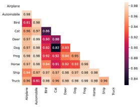
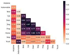
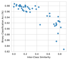
Figure 4: Matrices showing relationships among pairs of classes: (Left) binary classification accuracy matrix using EfficientNet-B0, (Middle) binary-class similarity matrix with $S_{2}$ metric, (Right) relationship between binary classification accuracy (left) and similarity scores (middle), plotted to show the high negative correlation between the two.

To further support the objectivity of our similarity measures, we compare similarity scores to accuracies for all pairwise classifications in CIFAR-10. The Pearson correlation coefficient between these two matrices is -0.77, showing strong correlation; it is negative because high accuracy corresponds with low similarity. All (similarity, accuracy) pairs are plotted on Figure 4 (right) clearly indicating the inverse relationship between similarity and accuracy. Notably, the lowest similarity data point is for the (automobile, deer) pair, and the highest similarity data point is for the (cat, dog) pair.

$ID_{c}$	0	1	2	3	4	5	6	7	8	9
$S_{1}$	0.73	0.80	0.82	0.85	0.92	0.92	0.99	1.00	0.71	0.83

Table 5: Intra-class similarity for CIFAR10. The class numbers $ID_{c}$ correspond to the class names in Figure 4

Intra-class similarity scores are shown for the same CIFAR-10 classes as in Table 5. All classes show high similarity scores with some differences. One can subjectively justify these numbers by visual examination. Classes 6 and 7 (dog and frog) have the highest similarity scores because foreground and background are similar for most images. Classes 0 and 8 (airplane and ship) have lower similarity scores because there is more diversity in foreground object and background.

5.5 Resolution and Scale, $R_{E}$ and $S_{C}$

In Table 1, the applications often downsize images to much smaller than the originals. Designers of these applications likely determined that accuracy didn’t suffer when images were reduced to the degree that they chose. This is also the case for our experiment of YOLOv5 nano on the COCO dataset in Figure 5 (left). One can see that accuracies drop slowly for image reduction from $640^{2}$ to $448^{2}$ – and further depending upon the degree of accuracy reduction that can be tolerated. Because scale drops with resolution, this plot includes the effects on accuracy reduction for both. In Figure 5 (right) we see the object detection performance almost flattens when reducing $R_{E}$ from 4k down to 1080p, and SY1-3 models’ accuracies are very close to nano but with about half the required computation (4.2 GFLOPs for nano versus 2.2 GFLOPs for SY3.

We also verify by experiment that $R_{E}$ has a direct impact on inference runtime per image  [45, 46]. Experiments on YOLOv5 nano in the COCO validation set are conducted, and results are shown in Table 6. One observation is that runtime almost doubles from 7.4ms for $1280^{2}$ to 13.4ms for $2560^{2}$ on a GPU, while it rises dramatically from 64.1 for $640^{2}$ to 4396.7 for $1280^{2}$ on a CPU.

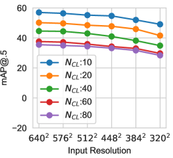
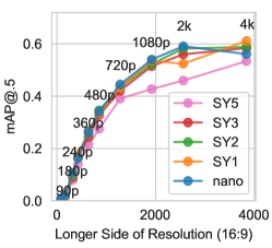
Figure 5: (Left) Effect of resolution on accuracy for YOLOv5-nano object detection on the COCO dataset, and (Right) effect on accuracy of YOLOv5 and sub-YOLO models for 80 classes of the PANDA 4k dataset  [47] .

$R_{E}$	$80^{2}$	$160^{2}$	$320^{2}$	$640^{2}$	$1280^{2}$	$2560^{2}$	$5120^{2}$
GPU	6.4	6.2	6.3	6.4	7.4	13.4	48.7
CPU	14.0	24.7	52.8	64.1	4396.7	4728.3	5456.9

Table 6: YOLOv5 runtimes [ms/img] for resolutions of the COCO validation set. Each number is averaged for 5 runs.

5.6 Robot Path Planning Application

We briefly mention results of methods from this paper used for efficient model design for our own application. The application is to detect times, locations, and densities of human activity on a factory floor for robot path planning. Initial labelling comprised 5 object classes: 2 of humans engaged in different activities, and 3 of different types of robots. Similarity metrics guided a reduction to 2 classes enabling a smaller model with computation reduction of 66% and accuracy gain of 3.5%. See [48] for a more complete description of this application.

6 Conclusion

We conclude that for applications requiring lightweight CNNs, data attributes can be examined and adjusted to obtain more efficient models. We examined four independent data-side variables, and results from our experiments indicate the following ranking upon computation reduction. Resolution has the greatest effect on computation. Most practitioners already perform resolution reduction, but many simply to fit the model of choice. We show that, for small (few-class) applications the model size can be reduced (to sub-YOLO models) to achieve more efficiency with similar accuracy, and this can be done efficiently using similarity metrics. Number of classes is second in rank. This is dependent on the application, but our methods using similarity metrics enable the application designer to compare different class groupings efficiently. We showed that the choice of color or grayscale had a relatively small (1-2%) effect on computation for small models. We don’t rank scale because scale was only tested with interdependency to resolution.

References

- [1] Olga Russakovsky, Jia Deng, Hao Su, Jonathan Krause, Sanjeev Satheesh, Sean Ma, Zhiheng Huang, Andrej Karpathy, Aditya Khosla, Michael Bernstein, Alexander C. Berg, and Li Fei-Fei. ImageNet Large Scale Visual Recognition Challenge. International Journal of Computer Vision (IJCV), 115(3):211–252, 2015.
- [2] Hung Nguyen, Sarah J. Maclagan, Tu Dinh Nguyen, Thin Nguyen, Paul Flemons, Kylie Andrews, Euan G. Ritchie, and Dinh Phung. Animal recognition and identification with deep convolutional neural networks for automated wildlife monitoring. In 2017 IEEE International Conference on Data Science and Advanced Analytics (DSAA), pages 40–49, 2017.
- [3] Yingfeng Cai, Tianyu Luan, Hongbo Gao, Hai Wang, Long Chen, Yicheng Li, Miguel Angel Sotelo, and Zhixiong Li. Yolov4-5d: An effective and efficient object detector for autonomous driving. IEEE Transactions on Instrumentation and Measurement, 70:1–13, 2021.
- [4] Fisher Yu, Haofeng Chen, Xin Wang, Wenqi Xian, Yingying Chen, Fangchen Liu, Vashisht Madhavan, and Trevor Darrell. Bdd100k: A diverse driving dataset for heterogeneous multitask learning, 2018.
- [5] Alex Krizhevsky, Ilya Sutskever, and Geoffrey E Hinton. Imagenet classification with deep convolutional neural networks. Advances in neural information processing systems, 25, 2012.
- [6] Karen Simonyan and Andrew Zisserman. Very deep convolutional networks for large-scale image recognition. arXiv preprint arXiv:1409.1556, 2014.
- [7] Soumya Sudhakar, Vivienne Sze, and Sertac Karaman. Data centers on wheels: Emissions from computing onboard autonomous vehicles. IEEE Micro, 43(1):29–39, 2023.
- [8] Yu Cheng, Duo Wang, Pan Zhou, and Tao Zhang. Model compression and acceleration for deep neural networks: The principles, progress, and challenges. IEEE Signal Processing Magazine, 93(8):863–878, 2018.
- [9] Forrest N Iandola, Song Han, Matthew W Moskewicz, Khalid Ashraf, William J Dally, and Kurt Keutzer. Squeezenet: Alexnet-level accuracy with 50x fewer parameters and< 0.5 mb model size. arXiv preprint arXiv:1602.07360, 2016.
- [10] Andrew G. Howard, Menglong Zhu, Bo Chen, Dmitry Kalenichenko, Weijun Wang, Tobias Weyand, Marco Andreetto, and Hartwig Adam. Mobilenets: Efficient convolutional neural networks for mobile vision applications. CoRR, abs/1704.04861, 2017.
- [11] Philipp Gysel, Jon Pimentel, Mohammad Motamedi, and Soheil Ghiasi. Ristretto: A framework for empirical study of resource-efficient inference in convolutional neural networks. IEEE transactions on neural networks and learning systems, 29(11):5784–5789, 2018.
- [12] Song Han, Huizi Mao, and William J Dally. Deep compression: Compressing deep neural networks with pruning, trained quantization and huffman coding. arXiv preprint arXiv:1510.00149, 2015.
- [13] Cong Leng, Zesheng Dou, Hao Li, Shenghuo Zhu, and Rong Jin. Extremely low bit neural network: Squeeze the last bit out with admm. In Proceedings of the AAAI conference on artificial intelligence, volume 32, 2018.
- [14] Yu Cheng, Duo Wang, Pan Zhou, and Tao Zhang. A survey of model compression and acceleration for deep neural networks. arXiv preprint arXiv:1710.09282, 2017.
- [15] Davis Blalock, Jose Javier Gonzalez Ortiz, Jonathan Frankle, and John Guttag. What is the state of neural network pruning? Proceedings of machine learning and systems, 2:129–146, 2020.
- [16] Hao Li, Asim Kadav, Igor Durdanovic, Hanan Samet, and Hans Peter Graf. Pruning filters for efficient convnets. arXiv preprint arXiv:1608.08710, 2016.
- [17] Maying Shen, Hongxu Yin, Pavlo Molchanov, Lei Mao, Jianna Liu, and Jose M Alvarez. Structural pruning via latency-saliency knapsack. arXiv preprint arXiv:2210.06659, 2022.
- [18] Serena Yeung, Olga Russakovsky, Greg Mori, and Li Fei-Fei. End-to-end learning of action detection from frame glimpses in videos. In Proceedings of the IEEE conference on computer vision and pattern recognition, pages 2678–2687, 2016.
- [19] Tsung-Yi Lin, Michael Maire, Serge Belongie, James Hays, Pietro Perona, Deva Ramanan, Piotr Dollár, and C Lawrence Zitnick. Microsoft coco: Common objects in context. In European conference on computer vision, pages 740–755. Springer, 2014.
- [20] Mark Everingham, Luc Van Gool, Christopher KI Williams, John Winn, and Andrew Zisserman. The pascal visual object classes (voc) challenge. International journal of computer vision, 88:303–308, 2009.
- [21] Joseph Redmon, Santosh Divvala, Ross Girshick, and Ali Farhadi. You only look once: Unified, real-time object detection. In Proceedings of the IEEE conference on computer vision and pattern recognition, pages 779–788, 2016.
- [22] Glenn Jocher et. al. ultralytics/yolov5: v6.0 - YOLOv5n ’Nano’ models, Roboflow integration, TensorFlow export, OpenCV DNN support, oct 2021.
- [23] Chien-Yao Wang, Alexey Bochkovskiy, and Hong-Yuan Mark Liao. Yolov7: Trainable bag-of-freebies sets new state-of-the-art for real-time object detectors. arXiv preprint arXiv:2207.02696, 2022.
- [24] Daniel Kang, John Emmons, Firas Abuzaid, Peter Bailis, and Matei Zaharia. Noscope: optimizing neural network queries over video at scale. arXiv preprint arXiv:1703.02529, 2017.
- [25] M. Fathy Z. Moayed R. Klette M. Sabokrou, M. Fayyaz. Deep-anomaly: Fully convolutional neural network for fast anomaly detection in crowded scenes. Computer Vision and Image Understanding, 172:88–97, 2018.
- [26] Shanwei Liu, Weimin Kong, Xingfeng Chen, Mingming Xu, Muhammad Yasir, Limin Zhao, and Jiaguo Li. Multi-scale ship detection algorithm based on a lightweight neural network for spaceborne sar images. Remote Sensing, 14(5), 2022.
- [27] T.T. Santos P.M. Santos J.G.A. Barbedo, L.V. Koenigkan. A study on the detection of cattle in uav images using deep learning. Sensors, 19(24), 2019.
- [28] Z. Han J. Huang W. Wang Y. Li, H. Wei. Deep learning-based safety helmet detection in engineering management based on convolutional neural networks. Advances in Civil Engineering, 2020:88–97, 2020.
- [29] H. Zhou C. Tian H. Qiang J. Zheng, X. Sun. Printed circuit boards defect detection method based on improved fully convolutional networks. IEEE Access, 10:109908–109918, 2022.
- [30] Zhenfeng Shao, Linggang Wang, Zhongyuan Wang, Wan Du, and Wenjing Wu. Saliency-aware convolution neural network for ship detection in surveillance video. IEEE Transactions on Circuits and Systems for Video Technology, 30(3):781–794, 2020.
- [31] P. Lejeune J. Linchant J. Théau A. Delplanque, S. Foucher. Multispecies detection and identification of african mammals in aerial imagery using convolutional neural networks. Remote Sensing in Ecology and Conservation, 8(April):166–179, 2022.
- [32] Gregory Koch, Richard Zemel, Ruslan Salakhutdinov, et al. Siamese neural networks for one-shot image recognition. In ICML deep learning workshop, volume 2, page 0. Lille, 2015.
- [33] Mat Kelcey. Metric learning for image similarity search (accessed: 2022/10/02).
- [34] Andreas Veit, Serge Belongie, and Theofanis Karaletsos. Conditional similarity networks. In Proceedings of the IEEE conference on computer vision and pattern recognition, pages 830–838, 2017.
- [35] Mariya I Vasileva, Bryan A Plummer, Krishna Dusad, Shreya Rajpal, Ranjitha Kumar, and David Forsyth. Learning type-aware embeddings for fashion compatibility. In Proceedings of the European conference on computer vision (ECCV), pages 390–405, 2018.
- [36] Reuben Tan, Mariya I Vasileva, Kate Saenko, and Bryan A Plummer. Learning similarity conditions without explicit supervision. In Proceedings of the IEEE/CVF international conference on computer vision, pages 10373–10382, 2019.
- [37] Andrew Zhai and Hao-Yu Wu. Classification is a strong baseline for deep metric learning. arXiv preprint arXiv:1811.12649, 2018.
- [38] Raia Hadsell, Sumit Chopra, and Yann LeCun. Dimensionality reduction by learning an invariant mapping. In 2006 IEEE Computer Society Conference on Computer Vision and Pattern Recognition (CVPR’06), volume 2, pages 1735–1742. IEEE, 2006.
- [39] Konstantin Kobs, Michael Steininger, Andrzej Dulny, and Andreas Hotho. Do different deep metric learning losses lead to similar learned features? In Proceedings of the IEEE/CVF International Conference on Computer Vision, pages 10644–10654, 2021.
- [40] Samarth Mishra, Zhongping Zhang, Yuan Shen, Ranjitha Kumar, Venkatesh Saligrama, and Bryan A Plummer. Effectively leveraging attributes for visual similarity. In Proceedings of the IEEE/CVF International Conference on Computer Vision, pages 1015–1024, 2021.
- [41] Alex Krizhevsky, Geoffrey Hinton, et al. Learning multiple layers of features from tiny images. 2009.
- [42] Mark Sandler, Andrew Howard, Menglong Zhu, Andrey Zhmoginov, and Liang-Chieh Chen. Mobilenetv2: Inverted residuals and linear bottlenecks. In Proceedings of the IEEE conference on computer vision and pattern recognition, pages 4510–4520, 2018.
- [43] Nermin Samet, Samet Hicsonmez, and Emre Akbas. Houghnet: Integrating near and long-range evidence for bottom-up object detection. In European Conference on Computer Vision (ECCV), 2020.
- [44] Hieu Minh Bui, Margaret Lech, Eva Cheng, Katrina Neville, and Ian S. Burnett. Using grayscale images for object recognition with convolutional-recursive neural network. In 2016 IEEE Sixth International Conference on Communications and Electronics (ICCE), pages 321–325, 2016.
- [45] Yue Meng, Chung-Ching Lin, Rameswar Panda, Prasanna Sattigeri, Leonid Karlinsky, Aude Oliva, Kate Saenko, and Rogerio Feris. Ar-net: Adaptive frame resolution for efficient action recognition. In European Conference on Computer Vision, pages 86–104. Springer, 2020.
- [46] Le Yang, Yizeng Han, Xi Chen, Shiji Song, Jifeng Dai, and Gao Huang. Resolution adaptive networks for efficient inference. In Proceedings of the IEEE/CVF conference on computer vision and pattern recognition, pages 2369–2378, 2020.
- [47] Xueyang Wang, Xiya Zhang, Yinheng Zhu, Yuchen Guo, Xiaoyun Yuan, Liuyu Xiang, Zerun Wang, Guiguang Ding, David Brady, Qionghai Dai, et al. Panda: A gigapixel-level human-centric video dataset. In Proceedings of the IEEE/CVF conference on computer vision and pattern recognition, pages 3268–3278, 2020.
- [48] Lawrence O'Gorman. Activity analytics from fixed cameras for robot path planning. TechRxiv, Jun 2022.