On the dynamics of the boundary vorticity
for incompressible viscous flows

Abstract

The dynamical equation of the boundary vorticity has been obtained, which shows that the viscosity at a solid wall is doubled as if the fluid became more viscous at the boundary. For certain viscous flows the boundary vorticity can be determined via the dynamical equation up to bounded errors for all time, without the need of knowing the details of the main stream flows. We then validate the dynamical equation by carrying out stochastic direct numerical simulations (i.e. the random vortex method for wall-bounded incompressible viscous flows) by two different means of updating the boundary vorticity, one using mollifiers of the Biot-Savart singular integral kernel, another using the dynamical equations.

Keywords: boundary vorticity, dynamical equation, incompressible fluid flow, stochastic integral representation, random vortex method

MSC classifications: 76M35, 76M23, 60H30, 65C05, 68Q10,

1 Introduction

When a viscous flow moves along a solid wall with large velocity, substantial molecular force takes effect among fluid particles at the boundary, and therefore vorticity is created instantly within a thin boundary layer, which in turn leads to substantial stress at the wall. The stress at the wall is indeed proportional to the vorticity created near the boundary, called the boundary vorticity for short. In many engineering applications, it is very important to understand the distribution of the stress over the boundary surface when a viscous fluid flow past a solid fluid boundary. It is important to obtain quantitative information of the stress distribution across the boundary at any instance for an unsteady viscous flow. Information about the boundary vorticity may be gained by performing numerical computations. The finite difference method or other numerical schemes may be used for solving numerically the fluid dynamics equations or the boundary layer equations, which however require to calculate the outer layer flows as well. It is therefore not cheap to carry out numerical experiments to acquire knowledge on the distribution of the boundary vorticity in general.

In this paper we propose a different approach to the study of the boundary vorticity of an incompressible viscous fluid flow past a solid wall, motivated by the recent work on the random vortex method for wall-bounded flows (cf. [11, 10]) via ordinary McKean-Vlasov type stochastic differential equations. In the random vortex methods for wall-bounded flows, the boundary stress has to be updated through iterations, and can not be assigned a priori. We instead in this work shall determine the dynamics of the boundary vorticity directly. The dynamical evolution equations for boundary vorticity for incompressible viscous fluid flows are obtained, which we believe is a new discovery. The dynamical equations of the boundary vorticity reveal several remarkable properties of incompressible viscous fluid flows at the boundary which we wish to report in this paper. It is revealed that the viscosity of the fluid flow is exactly doubled at the boundary as if the fluid became more viscous at the boundary. The dynamical equation of the boundary vorticity also demonstrates that the boundary vorticity evolves mainly linearly, in contrast to the high non-linearity of the Navier-Stokes equations. For some fluid flows, the boundary stress can be determined for all time with a bounded error, a fact which comes up a little bit surprising.

The paper is organised as the following. In Section 2, we write a formulation of the vorticity transport equation as a non-homogeneous boundary problem dependent on the boundary vorticity. The dynamical equation satisfied by the boundary vorticity is derived in Section 3. We write the stochastic representations of the vorticity and the velocity in terms of the Taylor diffusion in Section 4. Using these representations, we derive and implement a numerical scheme in Section 5 where the results of the conducted experiments are reported.

2 The fluid dynamics equations for flows past a wall

For a viscous fluid flow past a solid wall, it is clear that the geometry of the solid wall which constrains the fluid flow has a significant impact on the dynamics of the boundary vortices. As a matter of fact, the dynamics of the vortex motion at the solid wall becomes significantly complicated if the solid wall possesses non-trivial geometry (i.e., with non-constant curvature), and therefore the study for flows past curved surfaces will be published in a future work. In this article, we shall deal with viscous fluid flows past a flat plate, i.e. for the case the fluid boundary has trivial geometry.

Therefore we shall consider an incompressible fluid flow constrained in the upper half space $D=\mathbb{R}_{+}^{d}$ (where $d=2$ or $3$ in this work), the solid plate is modelled by the boundary $\partial D$ where $x_{d}=0$. Let $u=(u^{1},\ldots,u^{d})$ be the velocity and $P$ the pressure of the fluid flow in question. Then $u(x,t)$ is a time dependent vector field in $D$. The motion of the fluid is determined by the Navier-Stokes equations

$$\frac{\partial u}{\partial t}+(u\cdot\nabla)u-\nu\Delta u+\nabla P-F=0\quad\textrm{ in }D,$$ (2.1)

$$\nabla\cdot u=0\quad\textrm{ in }D,$$ (2.2)

together with the non-slip condition that $u(x,t)=0$ for $x\in\partial D$, where $F=(F^{1},\ldots,F^{d})$ is the external force applied to the fluid. The initial velocity of the flow is denoted by $u_{0}(x)$. The pressure is a scalar dynamic variable which is however determined by the velocity (up to a function depending only on $t$). Indeed, by taking the divergence of both sides of the first equation (2.1), i.e. applying $\frac{\partial}{\partial x_{i}}$ to this equation and summing up $i=1,\ldots,d$, one obtains

$$\Delta P=-\sum_{j,i=1}^{d}\frac{\partial u^{j}}{\partial x_{i}}\frac{\partial u^{i}}{\partial x_{j}}+\nabla\cdot F\quad\textrm{ in }D,$$ (2.3)

where we have used the divergence-free condition (2.2). The boundary value of $P$ remains to be determined. Since $u$ obeys the no-slip condition, so by reading the first equation (2.1) along the boundary $\partial D$ one obtains

$$\left.\nabla P\right|_{\partial D}=\nu\left.\Delta u\right|_{\partial D}+\left.F\right|_{\partial D}.$$ (2.4)

Instead of working out the boundary condition for $P$, we now consider the vorticity $\omega=\nabla\wedge u$ whose components $\omega^{j}=\varepsilon^{jki}\frac{\partial}{\partial x_{k}}u^{i}$ when $d=3$ and $\omega=\frac{\partial}{\partial x_{1}}u^{2}-\frac{\partial}{\partial x_{2}}u^{1}$ when $d=2$, which is in fact (up to a sign) the exterior derivative of $u$. Hence by applying the linear differential operator $\varepsilon^{jki}\frac{\partial}{\partial x_{k}}$ to both sides of (2.1), we shall obtain that

$$\frac{\partial}{\partial t}\omega+(u\cdot\nabla)\omega-\nu\Delta\omega-(\omega\cdot\nabla)u-G=0\quad\textrm{ in }D,$$ (2.5)

where $G=\nabla\wedge F$ with components $G^{j}=\varepsilon^{jki}\frac{\partial}{\partial x_{k}}F^{i}$ if $d=3$; if $d=2$, then $G=\frac{\partial}{\partial x_{1}}F^{2}-\frac{\partial}{\partial x_{2}}F^{1}$ and $(\omega\cdot\nabla)u=0$ identically.

In order to utilize the vorticity transport equation (2.5), we need to identify the boundary values of $\omega$, i.e. the boundary vorticity. Since $u$ obeys the non-slip condition, so that the normal part of $\omega$ at the boundary $\omega^{\perp}=\nabla^{\Gamma}\wedge u^{\parallel}=0$, where $u^{\|}$ denotes the tangential part of $u$ at the boundary, and $\nabla^{\Gamma}$ is the gradient operator in the boundary. For identifying the tangential part of $\omega$, we notice that the outwards unit normal $\boldsymbol{\nu}=-\frac{\partial}{\partial x_{3}}$. Hence

$$\left.\omega^{1}\right|_{\partial D}=\left.\frac{\partial u^{3}}{\partial x_{2}}-\frac{\partial u^{2}}{\partial x_{3}}\right|_{\partial D}=-\left.\frac{\partial u^{2}}{\partial x_{3}}\right|_{\partial D}=-2\left.S_{23}\right|_{\partial D}$$ (2.6)

and

$$\left.\omega^{2}\right|_{\partial D}=\left.\frac{\partial u^{1}}{\partial x_{3}}-\frac{\partial u^{3}}{\partial x_{1}}\right|_{\partial D}=\left.\frac{\partial u^{1}}{\partial x_{3}}\right|_{\partial D}=2\left.S_{13}\right|_{\partial D},$$ (2.7)

where

$$S_{ij}=\frac{1}{2}\left(\frac{\partial u^{i}}{\partial x_{j}}+\frac{\partial u^{j}}{\partial x_{i}}\right)$$

is the symmetric tensor field of rate-of-strain. Observe that the normal part of the symmetric tensor field $S=(S_{ij})$, denoted by $S^{\perp}$ is given by

$$S^{\perp}=\left.(S_{13},S_{23},S_{33})\right|_{\partial D}.$$

However, $\nabla\cdot u=0$, and $S_{11}=S_{22}=0$ on $\partial D$, hence $S_{33}=0$ too. Therefore $S^{\perp}$ can be identified with

$$S^{\perp}=\left.(S_{13},S_{23},0)\right|_{\partial D}$$

at the boundary. Therefore the boundary vorticity $\left.\omega\right|_{\partial D}$, denoted by $\theta$, is identified with twice of the stress at the boundary

$$\theta=\left.2(-S_{23},S_{13},0)\right|_{\partial D}.$$ (2.8)

Therefore the vorticity $\omega$ is evolved according to the following non-homogeneous boundary problem:

$$\begin{cases}\frac{\partial\omega}{\partial t}+(u\cdot\nabla)\omega-\nu\Delta\omega-(\omega\cdot\nabla)u-G=0&\textrm{ in }D,\\ \left.\omega\right|_{\partial D}-\theta=0&\textrm{ on }\partial D.\end{cases}$$ (2.9)

Note that the boundary vorticity $\theta$ is a tensor field on $\partial D$.

Remark 2.1.

The boundary vorticity $\theta$ can not be determined a priori, which causes a major problem for numerically computing solutions to the boundary value problem of the Navier-Stokes equations via the random vortex method (cf. [1, 3, 4, 5, 6, 8, 9]). While some authors supply instead the vorticity equations (2.5) with the Neumann boundary condition, which is in general not correct.

3 Dynamics of the boundary vorticity

In this section we shall derive the dynamical equation of the boundary vorticity $\theta$ which is the trace $\left.\omega\right|_{\partial D}$ of the vorticity $\omega$ at the boundary. To this end we assume that the velocity $u(x,t)$ is at least $C^{3}$ up to the boundary $\partial D$. Since $u$ satisfies the non-slip condition, by reading the vorticity equation (2.5) along $\partial D$ we therefore obtain

$$\frac{\partial\theta}{\partial t}-\nu\left.\Delta\omega\right|_{\partial D}-\left.(\theta\cdot\nabla)u\right|_{\partial D}-\psi=0\quad\textrm{ in }\partial D,$$ (3.1)

where $\psi=\left.G\right|_{\partial D}$, the boundary value of $G$. Using the non-slip condition again, we deduce that $\theta^{3}=0$ and

$$\left.(\theta\cdot\nabla)u\right|_{\partial D}=\left.\theta^{1}\frac{\partial u}{\partial x_{1}}\right|_{\partial D}+\left.\theta^{2}\frac{\partial u}{\partial x_{2}}\right|_{\partial D}=0.$$ (3.2)

We therefore have a very important consequence.

Theorem 3.1.

At the boundary, two non-linear terms appearing in the vorticity transport equation, the non-linear convection and the non-linear vorticity stretching, neither of them participates directly in the generation of the vorticity at the wall.

We are now in a position to state our main result of the paper.

Theorem 3.2.

Let $D=\mathbb{R}_{+}^{3}$. Then $\theta^{3}=0$, and $\theta^{1}$ and $\theta^{2}$ evolve according to the following dynamics:

$$\begin{cases}\frac{\partial\theta^{1}}{\partial t}-2\nu\Delta_{\Gamma}\theta^{1}+\nu\frac{\partial}{\partial x_{1}}\left(\nabla^{\Gamma}\cdot\theta\right)-\nu\left.\frac{\partial^{3}}{\partial\boldsymbol{\nu}^{3}}u^{2}\right|_{\partial D}-\psi^{1}=0\\ \frac{\partial\theta^{2}}{\partial t}-2\nu\Delta_{\Gamma}\theta^{2}+\nu\frac{\partial}{\partial x_{2}}\left(\nabla^{\Gamma}\cdot\theta\right)+\nu\left.\frac{\partial^{3}}{\partial\boldsymbol{\nu}^{3}}u^{1}\right|_{\partial D}-\psi^{2}=0\end{cases}$$ (3.3)

in $\partial D=\mathbb{R}^{2}$. That is

$$\frac{\partial\theta}{\partial t}-2\nu\Delta_{\Gamma}\theta+\nu\nabla^{\Gamma}\left(\nabla^{\Gamma}\cdot\theta\right)+\nu\star\left.\frac{\partial^{3}}{\partial\boldsymbol{\nu}^{3}}u^{\parallel}\right|_{\partial D}-\psi=0.$$ (3.4)

Here $\boldsymbol{\nu}$ is the normal to $\partial D$ pointing outward, i.e. $\boldsymbol{\nu}=-\frac{\partial}{\partial x_{3}}$, $\Delta_{\Gamma}$ and $\nabla^{\Gamma}$ denote the Laplacian and gradient operator on $\mathbb{R}^{2}$ respectively. Here $\star$ is the Hodge star operator of $\partial D$, and $u^{\parallel}$ is the tangential extension, in this case, $u^{\parallel}=(u^{1},u^{2})$.

Before we give the derivation of the boundary vorticity dynamics, we would like to make several comments.

Remark 3.3.

The dynamical equations (3.3) imply that the kinematic viscosity constant at the boundary is exactly doubled, as if the fluid became more ‘viscous’ than the fluid in the main stream. This phenomenon is actually true for any viscous wall-bounded flow constrained by a curved solid wall.

Remark 3.4.

The motion equation (3.4) for the boundary vorticity also indicates clearly how the external flow (i.e., the flow away from the boundary) participates in the generation of the vorticity at the boundary. More precisely, the boundary vorticity is generated, with the help of the initial boundary vorticity and the external boundary force $\psi$, together with an ‘external’ force $-\nu\star\left.\frac{\partial^{3}}{\partial\boldsymbol{\nu}^{3}}u^{\parallel}\right|_{\partial D}$ from the main stream flow exerted on the "self-dynamics" of the boundary vorticity, which is determined by the linear heat operator

$$\frac{\partial\theta}{\partial t}-2\nu\Delta_{\Gamma}\theta+\nu\nabla^{\Gamma}\left(\nabla^{\Gamma}\cdot\theta\right).$$

Remark 3.5.

For a typical wall-bounded viscous fluid flow, in particular for turbulent boundary layer flows, the boundary vorticity $(\theta^{1},\theta^{2})$ (which equals the normal stress at the boundary) is significant, which is big in comparison with the typical scale of the flow. While the ‘external’ force inherited from the outer layer flow, which adjusts the self-dynamics of the boundary vorticity, is proportional to the kinematic viscosity $\nu$. Since the dynamical equation

$$\frac{\partial\tilde{\theta}}{\partial t}-2\nu\Delta_{\Gamma}\tilde{\theta}+\nu\nabla^{\Gamma}\left(\nabla^{\Gamma}\cdot\tilde{\theta}\right)-\psi=0$$

subject to the same initial boundary vorticity $\tilde{\theta}=\theta$ at $t=0$, is linear, hence if $\left.\frac{\partial^{3}}{\partial\boldsymbol{\nu}^{3}}u^{\parallel}\right|_{\partial D}$ is bounded and the kinematic viscosity $\nu$ is small, then the boundary vorticity $\theta(x,t)$ is more or less self-organised, and the outer layer flow inserts insignificant impact on the generation of the boundary vorticity.

Proof.

[of Theorem 3.2] The proof is completely elementary. We begin with Eq. (3.1) and we need to compute the trace of $\Delta\omega$ at the boundary. While it is clear that

$$\left.\Delta\omega^{i}\right|_{\partial D}=\left.\left(\frac{\partial^{2}}{\partial x_{1}^{2}}+\frac{\partial^{2}}{\partial x_{2}^{2}}\right)\omega^{i}+\frac{\partial^{2}}{\partial x_{3}^{2}}\omega^{i}\right|_{\partial D}=\Delta_{\Gamma}\theta^{i}+\left.\frac{\partial^{2}}{\partial x_{3}^{2}}\omega^{i}\right|_{\partial D}$$

where the last term has to be computed. While

$$\frac{\partial}{\partial x_{3}}\omega^{1} =\frac{\partial}{\partial x_{3}}\left(\frac{\partial u^{3}}{\partial x_{2}}-\frac{\partial u^{2}}{\partial x_{3}}\right)=\frac{\partial}{\partial x_{3}}\frac{\partial u^{3}}{\partial x_{2}}-\frac{\partial}{\partial x_{3}}\frac{\partial}{\partial x_{3}}u^{2}$$

$$=-\frac{\partial}{\partial x_{2}}\left(\frac{\partial u^{1}}{\partial x_{1}}+\frac{\partial u^{2}}{\partial x_{2}}\right)-\frac{\partial}{\partial x_{3}}\frac{\partial}{\partial x_{3}}u^{2}$$

and therefore

$$\frac{\partial^{2}}{\partial x_{3}^{2}}\omega^{1} =\frac{\partial^{2}}{\partial x_{3}^{2}}\left(\frac{\partial}{\partial x_{2}}u^{3}-\frac{\partial}{\partial x_{3}}u^{2}\right)$$

$$=\frac{\partial^{2}}{\partial x_{2}\partial x_{3}}\frac{\partial}{\partial x_{3}}u^{3}-\frac{\partial^{2}}{\partial x_{3}^{2}}\frac{\partial}{\partial x_{3}}u^{2}$$

$$=-\frac{\partial^{2}}{\partial x_{2}\partial x_{3}}\frac{\partial}{\partial x_{1}}u^{1}-\frac{\partial^{2}}{\partial x_{2}\partial x_{3}}\frac{\partial}{\partial x_{2}}u^{2}-\frac{\partial^{2}}{\partial x_{3}^{2}}\frac{\partial}{\partial x_{3}}u^{2}$$

$$=\frac{\partial^{2}}{\partial x_{2}^{2}}\omega^{1}+\frac{\partial^{2}}{\partial x_{1}^{2}}\omega^{1}-\frac{\partial^{2}}{\partial x_{1}^{2}}\omega^{1}-\frac{\partial^{2}}{\partial x_{2}\partial x_{1}}\omega^{2}-\frac{\partial^{2}}{\partial x_{3}^{2}}\frac{\partial}{\partial x_{3}}u^{2}$$

$$=\Delta_{\Gamma}\theta^{1}-\frac{\partial}{\partial x_{1}}\left(\nabla_{\Gamma}\cdot\theta\right)-\frac{\partial^{2}}{\partial x_{3}^{2}}\frac{\partial}{\partial x_{3}}u^{2}$$

It follows that

$$\left.\frac{\partial^{2}}{\partial x_{3}^{2}}\omega^{1}\right|_{\partial D}=-\frac{\partial^{3}}{\partial x_{3}^{3}}u^{2}+\Delta_{\Gamma}\theta^{1}-\frac{\partial}{\partial x_{1}}\left(\nabla_{\Gamma}\cdot\theta\right).$$

Similarly

$$\frac{\partial^{2}}{\partial x_{3}^{2}}\omega^{2} =\frac{\partial^{2}}{\partial x_{3}^{2}}\left(\frac{\partial}{\partial x_{3}}u^{1}-\frac{\partial}{\partial x_{1}}u^{3}\right)$$

$$=-\frac{\partial^{2}}{\partial x_{1}\partial x_{3}}\frac{\partial}{\partial x_{3}}u^{3}+\frac{\partial^{2}}{\partial x_{3}^{2}}\frac{\partial}{\partial x_{3}}u^{1}$$

$$=\frac{\partial^{2}}{\partial x_{1}\partial x_{3}}\frac{\partial}{\partial x_{1}}u^{1}+\frac{\partial^{2}}{\partial x_{1}\partial x_{3}}\frac{\partial}{\partial x_{2}}u^{2}+\frac{\partial^{2}}{\partial x_{3}^{2}}\frac{\partial}{\partial x_{3}}u^{1}$$

$$=\frac{\partial^{2}}{\partial x_{1}^{2}}\omega^{2}+\frac{\partial^{2}}{\partial x_{2}^{2}}\omega^{2}-\frac{\partial^{2}}{\partial x_{2}^{2}}\omega^{2}-\frac{\partial^{2}}{\partial x_{2}\partial x_{1}}\omega^{1}+\frac{\partial^{2}}{\partial x_{3}^{2}}\frac{\partial}{\partial x_{3}}u^{1}$$

$$=\Delta_{\Gamma}\theta^{2}-\frac{\partial}{\partial x_{2}}\left(\nabla_{\Gamma}\cdot\theta\right)+\frac{\partial^{2}}{\partial x_{3}^{2}}\frac{\partial}{\partial x_{3}}u^{1}$$

where the second equality follows from the divergence-free: $\nabla\cdot u=0$. Hence

$$\left.\frac{\partial}{\partial x_{3}}\omega^{1}\right|_{\partial D}=-\left.\frac{\partial}{\partial x_{3}}\frac{\partial}{\partial x_{3}}u^{2}\right|_{\partial D}$$ (3.5)

and

$$\left.\frac{\partial}{\partial x_{3}}\omega^{2}\right|_{\partial D}=\left.\frac{\partial}{\partial x_{3}}\frac{\partial}{\partial x_{3}}u^{1}\right|_{\partial D}.$$ (3.6)

so that

$$\left.\frac{\partial^{2}}{\partial x_{3}^{2}}\omega^{2}\right|_{\partial D}=\frac{\partial^{3}}{\partial x_{3}^{3}}u^{1}+\Delta_{\Gamma}\theta^{1}-\frac{\partial}{\partial x_{2}}\left(\nabla_{\Gamma}\cdot\theta\right).$$

Similarly

$$\frac{\partial}{\partial x_{3}}\omega^{3} =\frac{\partial}{\partial x_{3}}\left(\frac{\partial u^{2}}{\partial x_{1}}-\frac{\partial u^{1}}{\partial x_{2}}\right)=\frac{\partial}{\partial x_{3}}\frac{\partial u^{2}}{\partial x_{1}}-\frac{\partial}{\partial x_{3}}\frac{\partial}{\partial x_{2}}u^{1}$$

$$=\frac{\partial}{\partial x_{1}}\frac{\partial u^{2}}{\partial x_{3}}-\frac{\partial}{\partial x_{2}}\frac{\partial u^{1}}{\partial x_{3}}$$

$$=-\left(\frac{\partial}{\partial x_{1}}\omega^{1}+\frac{\partial}{\partial x_{2}}\omega^{2}\right)-\frac{\partial}{\partial x_{2}}\frac{\partial u^{3}}{\partial x_{1}}+\frac{\partial}{\partial x_{1}}\frac{\partial u^{3}}{\partial x_{2}}$$

and

$$\frac{\partial^{2}}{\partial x_{3}^{2}}\omega^{3}=-\frac{\partial}{\partial x_{3}}\left(\frac{\partial}{\partial x_{1}}\omega^{1}+\frac{\partial}{\partial x_{2}}\omega^{2}\right)$$

so that

$$\left.\frac{\partial}{\partial x_{3}}\omega^{3}\right|_{\partial D}=-\nabla^{\Gamma}\cdot\theta=-\frac{\partial\theta^{1}}{\partial x_{1}}-\frac{\partial\theta^{2}}{\partial x_{2}}.$$ (3.7)

Putting these equations together we obtain (3.3). ∎

For convenience let us write down the evolution for two dimensional flows for reference below.

Theorem 3.6.

If $d=2$ (so that both $\omega=\frac{\partial}{\partial x_{1}}u^{2}-\frac{\partial}{\partial x_{2}}u^{1}$ and its trace $\theta$ at the boundary are scalar function), then the boundary vorticity $\theta$ evolves according to the following dynamical equation

$$\frac{\partial\theta}{\partial t}-2\nu\Delta_{\Gamma}\theta-\nu\left(\frac{\partial}{\partial\boldsymbol{\nu}}\right)^{3}u^{\|}-\psi=0$$ (3.8)

where $u^{\|}=u^{1}$ is the tangent component of the velocity field $u$.

Proof.

In this case we prefer use coordinates $x=(x_{1},x_{2})$. For 2D flow, the vorticity transport equation becomes

$$\frac{\partial\omega}{\partial t}+(u\cdot\nabla)\omega-\nu\Delta\omega=G\quad\textrm{ in }D$$ (3.9)

where $\omega=\frac{\partial u^{2}}{\partial x_{1}}-\frac{\partial u^{1}}{\partial x_{2}}$, so that

$$\Delta\omega =\frac{\partial^{2}}{\partial x_{1}^{2}}\omega+\frac{\partial^{2}}{\partial x_{2}^{2}}\left(\frac{\partial u^{2}}{\partial x_{1}}-\frac{\partial u^{1}}{\partial x_{2}}\right)$$

$$=2\frac{\partial^{2}}{\partial x_{1}^{2}}\omega-\frac{\partial^{3}}{\partial x_{1}^{3}}u^{2}-\frac{\partial^{3}}{\partial x_{2}^{3}}u^{1}$$

so that

$$\left.\Delta\omega\right|_{\partial D}=2\Delta_{\Gamma}\theta+\left(\frac{\partial}{\partial\boldsymbol{\nu}}\right)^{3}u^{1}$$

and the conclusion follows immediately. ∎

4 Functional integral representations

In the next two sections we demonstrate the use of the dynamical equations in the stochastic direct numerical simulations of the viscous flows within thin layers next to the fluid boundary.

We shall develop random vortex schemes for calculating numerically solutions to the boundary problem (2.1, 2.2) by using the dynamical equations of the boundary vorticity for updating the boundary values of the vorticity in numerical schemes.

To exhibit our ideas clearly we deal with 2D flows only, i.e. $d=2$ and $D=\{x:x_{2}>0\}$. Since the boundary vorticity $\theta$ is in general non-trivial, so we introduce a family of perturbations of $\omega$ defined by $W^{\varepsilon}=\omega-\sigma_{\varepsilon}$ for every $\varepsilon>0$, given by

$$\sigma_{\varepsilon}(x_{1},x_{2},t)=\theta(x_{1},t)\phi(x_{2}/\varepsilon),$$ (4.1)

where $\phi:[0,\infty)\rightarrow[0,1]$ is a proper cut-off function such that $\phi(r)=1$ for $r\in[0,1/3)$ and $\phi(r)=0$ for $r\geq 2/3$. Indeed we will use the following cut-off function:

$$\phi(r)=\begin{cases}1&\textrm{for $r\in[0,1/3)$,}\\ \frac{1}{2}+54\left(r-\frac{1}{2}\right)^{3}-\frac{9}{2}\left(r-\frac{1}{2}\right)&\textrm{ for }r\in[1/3,2/3],\\ 0&\textrm{ for }r\geq 2/3\end{cases}$$ (4.2)

Hence $-54\leq\phi^{\prime\prime}\leq 54$, $-\frac{9}{2}\leq\phi^{\prime}\leq 0$ on $[1/3,2/3]$ and $\phi^{\prime}=0$ for $r\leq 1/3$ or $r\geq 2/3$. In fact

$$\phi^{\prime}(r)=\begin{cases}162\left(r-\frac{1}{2}\right)^{2}-\frac{9}{2}&\textrm{ for }r\in[1/3,2/3],\\ 0&\textrm{ otherwise }\end{cases}$$ (4.3)

and

$$\phi^{\prime\prime}(r)=\begin{cases}324\left(r-\frac{1}{2}\right)&\textrm{ for }r\in[1/3,2/3],\\ 0&\textrm{ otherwise. }\end{cases}$$ (4.4)

Then $W_{\varepsilon}$ is the solution to the following Dirichlet boundary problem of the parabolic equation:

$$\left(\frac{\partial}{\partial t}+u\cdot\nabla-\nu\Delta\right)W_{\varepsilon}-g_{\varepsilon}=0\quad\textrm{ in }D,\quad\textrm{ and }\left.W_{\varepsilon}\right|_{\partial D}=0,$$ (4.5)

where

$$g_{\varepsilon}(x,t) =G(x,t)+\frac{\nu}{\varepsilon^{2}}\phi^{\prime\prime}(x_{2}/\varepsilon)\theta(x_{1},t)-\frac{1}{\varepsilon}\phi^{\prime}(x_{2}/\varepsilon)u^{2}(x,t)\theta(x_{1},t)$$

$$+\phi(x_{2}/\varepsilon)\left(\nu\frac{\partial^{2}\theta}{\partial x_{1}^{2}}(x_{1},t)-\frac{\partial\theta}{\partial t}(x_{1},t)\right)-\phi(x_{2}/\varepsilon)u^{1}(x,t)\frac{\partial\theta}{\partial x_{1}}(x_{1},t)$$ (4.6)

for any $x=(x_{1},x_{2})$, $x_{2}>0$. The initial data for $W^{\varepsilon}$ is given by

$$W_{0}^{\varepsilon}(x)=\omega_{0}(x_{1},x_{2})-\omega_{0}(x_{1},0)\phi(x_{2}/\varepsilon)\quad\textrm{ for }x\in D.$$ (4.7)

We shall need the stochastic integral representation in terms of the Taylor diffusion with velocity $u(x,t)$. To this end, the vector field $u(x,t)$ is extended to a vector field on $\mathbb{R}^{2}$ by reflection about the line $x_{2}=0$ so that

$$u^{1}(x,t)=u^{1}(\overline{x},t),\quad u^{2}(x,t)=-u^{2}(\overline{x},t)$$

for $x=(x_{1},x_{2})$ with $x_{2}>0$, here $x\mapsto\overline{x}$ is the reflection about the line that $x_{2}=0$, that is, $\overline{x}=(x_{1},-x_{2})$ for $x=(x_{1},x_{2})\in\mathbb{R}^{2}$. This extension retains the divergence-free property, though, in distribution. That is, $\nabla\cdot u(\cdot,t)=0$ on $\mathbb{R}^{2}$ in the sense of distribution.

For each $\xi\in\mathbb{R}^{2}$, $(X_{t}^{\xi})_{t\geq 0}$ is the unique (weak) solution of the following Itô’s stochastic differential equation

$$\textrm{d}X_{t}^{\xi}=u(X_{t}^{\xi},t)\textrm{d}t+\sqrt{2\nu}\textrm{d}B_{t},\quad X_{0}^{\xi}=\xi,$$ (4.8)

where $B=(B_{t})$ is a two dimensional Brownian motion on some probability space. Let $p(s,\xi;t,y)$ be the transition probability density function of the diffusion $(X_{t}^{\xi})_{t\geq 0}$, i.e.

$$p(s,x;t,y)\textrm{d}y=\mathbb{P}\left[\left.X_{t}^{\xi}\in\textrm{d}y\right|X_{s}^{\xi}=x\right]$$

for $t>s\geq 0$ and $x,y\in\mathbb{R}^{2}$ (which is independent of $\xi$). Let $p^{D}(s,x;t,y)$ be the transition (sub-)probability density function of the diffusion $X^{\xi}$ killed on leaving the region $D$, where $t>s\geq 0$, $x,y\in D$. Then

$$p^{D}(s,x;t,y)\textrm{d}y=\mathbb{P}\left[\left.1_{\left\{\zeta(X^{\eta})>t\right\}},X_{t}^{\xi}\in\textrm{d}y\right|X_{s}^{\xi}=x\right]$$

for any $t>s\geq 0$, and

$$p^{D}(s,x;t,y)=p(s,x;t,y)-p(s,x;t,\bar{y})$$ (4.9)

for $t>s\geq 0$ and $x,y\in D$, where $\zeta(\psi)=\inf\left\{t:\psi(t)\notin D\right\}$. Note that, since $\overline{u(x,t)}=u(\bar{x},t)$ for $x\in\mathbb{R}^{2}$ and $t\geq 0$, $p(s,x;t,y)=p(s,\bar{x};t,\bar{y})$.

Theorem 4.1.

For every $\varepsilon>0$, it holds that

$$W_{\varepsilon}(y,t)= \int_{D}\mathbb{P}\left[\left.\zeta(X^{\eta})>t\right|X_{t}^{\eta}=y\right]W_{\varepsilon}(\eta,0)p(0,\eta;t,y)\textrm{d}\eta$$

$$+\int_{0}^{t}\int_{D}\mathbb{E}\left[\left.1_{\left\{s>\gamma_{t}(X^{\eta})\right\}}g_{\varepsilon}(X_{s}^{\eta},s)\right|X_{t}^{\eta}=y\right]p(0,\eta;t,y)\textrm{d}\eta\textrm{d}s$$ (4.10)

for every $t>0$ and $y\in D$, where $\gamma_{t}(\psi)=\sup\left\{s\in(0,t):\psi(s)\notin D\right\}$ for every continuous path $\psi$.

For a proof of this representation, we refer to [10] and [7]. We emphasize that the previous representation (4.10) is different from the solution representation in terms of the fundamental solution in that only the Taylor diffusion starting at a fixed time $0$ is required, which therefore reduces the computational cost substantially when numerical schemes are implemented based on such integral representations.

We next establish a representation for $u(x,t)$ by applying the Biot-Savart law. To this end, we apply the following convention. For 2D vectors, the following convention, which is consistent with the canonical identifications with 3D vectors, will be adopted. If $a=(a_{1},a_{2})$ and $b=(b_{1},b_{2})$, then $a\wedge b=a_{1}b_{2}-a_{2}b_{1}$ (a scalar), and if $c$ is a scalar, then $a\wedge c=(a_{2}c,-a_{1}c)$.

Theorem 4.2.

The following stochastic integral representation for the velocity holds:

$$u(x,t) =\int_{D}K(y,x)\wedge\sigma_{\varepsilon}(y,t)\textrm{d}y$$

$$+\int_{D}\mathbb{E}\left[1_{D}(X_{t}^{\xi})K(X_{t}^{\xi},x)-1_{D}(X_{t}^{\bar{\xi}})K(X_{t}^{\bar{\xi}},x)\right]\wedge W_{\varepsilon}(\xi,0)\textrm{d}\xi$$

$$+\int_{0}^{t}\int_{D}\mathbb{E}\left[\left.1_{\left\{s>\gamma_{t}(X^{\eta})\right\}}K(X_{t}^{\eta},x)\wedge g_{\varepsilon}(X_{s}^{\eta},s)\right|\right]\textrm{d}\eta\textrm{d}s$$ (4.11)

for every $x\in D$, and $u(x,t)=\overline{u(\overline{x},t)}$ for $x_{2}<0$, and $u(x,t)=0$ if $x_{2}=0$.

Proof.

Recall that the Biot-Savart singular integral kernel for $D$ (which is the gradient of the green function for $D$) is given by

$$K(y,x)=\frac{1}{2\pi}\left(\frac{y-x}{|y-x|^{2}}-\frac{y-\overline{x}}{|y-\overline{x}|^{2}}\right)$$ (4.12)

for $y\neq x$ or $\overline{x}$. Since $\nabla\cdot u=0$, $\nabla\wedge u=\omega$ and $u$ is subject to the Dirichlet boundary condition that $u(x,t)=0$ for $x\in\partial D$, hence, according to Green formula we obtain that

$$u(x,t)=\int_{D}K(y,x)\wedge\omega(y,t)\textrm{d}y.$$ (4.13)

While by definition, for every $\varepsilon>0$, $\omega=\sigma_{\varepsilon}+W_{\varepsilon}$, the representation follows by utilising the representation (4.10) and the Fubini theorem. ∎

5 Numerical experiments

In this section, we provide some numerical simulations for the representations discussed above, focusing on the two-dimensional case. Recall that, by letting $\epsilon\downarrow 0$ in (4.11) the following representation holds:

$$u(x,t) =\int_{D}K^{\perp}(x,\eta)\sigma_{\varepsilon}(\eta,t)\textrm{d}\eta+\int_{D}\mathbb{E}\left[K^{\perp}(x,X_{t}^{\eta})1_{\left\{t<\zeta(X^{\eta}\circ\tau_{t})\right\}}\right]\omega_{0}(\eta)\textrm{d}\eta$$

$$-\int_{D}\mathbb{E}\left[K^{\perp}(x,X_{t}^{\eta})1_{\left\{t<\zeta(X^{\eta}\circ\tau_{t})\right\}}\right]\sigma_{\varepsilon}(\eta,t)\textrm{d}\eta$$

$$+\int_{0}^{t}\int_{D}\mathbb{E}\left[1_{\{t-s<\zeta(X^{\eta}\circ\tau_{t})\}}K^{\perp}(x,X_{t}^{\eta})G(X_{s}^{\eta},s)\right]\textrm{d}\eta\textrm{d}s$$

$$+\int_{0}^{t}\int_{D}\mathbb{E}\left[1_{\{t-s<\zeta(X^{\eta}\circ\tau_{t})\}}K^{\perp}(x,X_{t}^{\eta})\rho_{\varepsilon}(X_{s}^{\eta},s)\right]\textrm{d}\eta\textrm{d}s,$$ (5.1)

where $\rho_{\varepsilon}=g_{\varepsilon}-G$ and

$$K^{\perp}=(K^{2},-K^{1})$$ (5.2)

in our notation. In the following we ease the notation by omitting the superscript in the kernel and the wedge product coming from the Biot-Savart law (4.13), which is essentially equivalent to redefining the kernel as in (5.2).

The only term in the definition of $\rho_{\varepsilon}(x,t)$, dependent on $\varepsilon$, that does not vanish in the limit is

$$\frac{\nu}{\varepsilon^{2}}\phi^{\prime\prime}(x_{2}/\varepsilon)\theta(x_{1},t).$$ (5.3)

Therefore, one can approximate the representation for the velocity $u$ by the following

$$u^{i}(x,t) \approx\int_{D}\mathbb{E}\left[1_{\left\{t<\zeta(X^{\eta}\circ\tau_{t})\right\}}K^{i}(x,X_{t}^{\xi})\right]\omega_{0}(\xi)\textrm{d}\xi$$

$$+\int_{0}^{t}\int_{D}\mathbb{E}\left[1_{\{t-s<\zeta(X^{\xi}\circ\tau_{t})\}}K^{i}(x,X_{t}^{\xi})G(X_{s}^{\xi},s)\right]\textrm{d}\xi\textrm{d}s$$

$$+\frac{\nu}{\varepsilon^{2}}\int_{0}^{t}\int_{D}\mathbb{E}\left[1_{\{t-s<\zeta(X^{\xi}\circ\tau_{t})\}}K^{i}(x,X_{t}^{\xi})\theta(X_{s}^{\xi},s)\phi^{\prime\prime}(X_{s}^{\xi}/\varepsilon)\right]\textrm{d}\xi\textrm{d}s,$$ (5.4)

for some small $\varepsilon$. That is, we omit the terms that do not contribute to the limit and (5.3) is approximated by taking sufficiently small $\varepsilon$. Notice that as the support of $\phi^{\prime\prime}$ is the interval $[1/3,2/3]$, the last integration can be taken over a thin layer close to the boundary. Notice also that in the last integration we used $\theta(x,s),\phi^{\prime\prime}(x/\varepsilon)$ to denote $\theta(x_{1},s),\phi^{\prime\prime}(x_{2}/\varepsilon)$ slightly abusing notation.

We use the idea described above to the representation (4.11), i.e. we approximate the velocity similarly as

$$u(x,t) \approx\int_{D}\mathbb{E}\left[1_{D}(X_{t}^{\xi})K(X_{t}^{\xi},x)-1_{D}(X_{t}^{\bar{\xi}})K(X_{t}^{\bar{\xi}},x)\right]\omega_{0}(\xi)\textrm{d}\xi$$

$$+\int_{0}^{t}\int_{D}\mathbb{E}\left[1_{\left\{s>\gamma_{t}(X^{\eta})\right\}}K(X_{t}^{\eta},x)G(X_{s}^{\eta},s)\right]\textrm{d}\eta\textrm{d}s$$

$$+\frac{\nu}{\varepsilon^{2}}\int_{0}^{t}\int_{D}\mathbb{E}\left[1_{\left\{s>\gamma_{t}(X^{\eta})\right\}}K(X_{t}^{\eta},x)\theta(X_{s}^{\eta},s)\phi^{\prime\prime}(X_{s}^{\eta}/\varepsilon)\right]\textrm{d}\eta\textrm{d}s,$$ (5.5)

for every $x\in D$, and $u(x,t)=\overline{u(\overline{x},t)}$ for $x_{2}<0$, and $u(x,t)=0$ if $x_{2}=0$.

For the half-plane domain $D$, we introduce lattice points as follows. Notice that as in (5) the first integral contains processes with reflected initial positions $\bar{\xi}$, we have to add reflected lattice points for the below discretisation.

1. The thin boundary layer lattice $D_{b}$ is given by

   $$x_{b}^{i_{1}i_{2}}=(i_{1}h_{1},i_{2}h_{2}),\quad\text{ for }-N_{1}\leq i_{1}\leq N_{1}\text{ and }-N_{2}\leq i_{2}\leq N_{2},$$ (5.6)

   where $h_{1},h_{2}$ are mesh sizes and $N_{1},N_{2}$ are numbers of points.

2. The outer layer lattice $D_{o}$ is defined as

   $$x_{o}^{i_{1}i_{2}}=(i_{1}h_{0},i_{2}h_{0}),\quad\text{ for }-N_{0}\leq i_{1}\leq N_{0}\text{ and }-N_{2}\leq i_{2}\leq N_{2},$$ (5.7)

   where $h_{0}$ is mesh size and $N_{0}$ is the number of points.

The discretised random vortex system is described as follows. We initialise the processes $X^{i_{1},i_{2}}_{b;t_{0}}=x_{b}^{i_{1}i_{2}}$ and $X^{i_{1},i_{2}}_{o;t_{0}}=x_{o}^{i_{1}i_{2}}$ and update them for $k\geq 0$ according to

$$X^{i_{1},i_{2}}_{t_{k+1}}=X^{i_{1},i_{2}}_{t_{k}}+h\hat{u}(X^{i_{1},i_{2}}_{t_{k}},t_{k})+\sqrt{2\nu}(B_{t_{k+1}}-B_{t_{k}}),$$ (5.8)

where $t_{k}=kh$ for $k\geq 0$ and some fixed time mesh $h$. To ease the notation, we drop the subscripts $o$ and $b$. The processes are coupled with the drift $\hat{u}$ which is given by

$$\hat{u}(x,t_{k+1}) =\sum_{\begin{subarray}{c}(i_{1},i_{2})\in D\\ i_{2}>0\end{subarray}}A_{i_{1},i_{2}}\omega_{i_{1},i_{2}}\mathbb{E}\left[1_{D}(X^{i_{1},i_{2}}_{t_{k}})K(X^{i_{1},i_{2}}_{t_{k}},x)-1_{D}(X^{i_{1},-i_{2}}_{t_{k}})K(X^{i_{1},-i_{2}}_{t_{k}},x)\right]$$

$$+\sum_{\begin{subarray}{c}(i_{1},i_{2})\in D\\ i_{2}>0\end{subarray}}\sum_{l=0}^{k}A_{i_{1},i_{2}}hG_{i_{1},i_{2};t_{l}}\mathbb{E}\left[1_{\left\{t_{l}>\gamma_{t_{k}}(X^{i_{1},i_{2}})\right\}}K(X^{i_{1},i_{2}}_{t_{k}},x)G(X^{i_{1},i_{2}}_{t_{l}},t_{l})\right]$$

$$+\frac{\nu}{\varepsilon^{2}}\sum_{\begin{subarray}{c}(i_{1},i_{2})\in D_{b}\\ i_{2}>0\end{subarray}}\sum_{l=0}^{k}h_{1}h_{2}h\mathbb{E}\left[1_{\left\{t_{l}>\gamma_{t_{k}}(X^{i_{1},i_{2}})\right\}}K(X^{i_{1},i_{2}}_{t_{k}},x)\theta(X^{i_{1},i_{2}}_{t_{l}},t_{l})\phi^{\prime\prime}(X^{i_{1},i_{2}}_{t_{l}}/\varepsilon)\right],$$ (5.9)

for $x\in D$, and $\hat{u}(x,t)=\overline{\hat{u}(\overline{x},t)}$ for $x_{2}<0$, and $\hat{u}(x,t)=0$ if $x_{2}=0$. In what follows, we unify summations over $(i_{1},i_{2})\in D_{o}$ and $(i_{1},i_{2})\in D_{b}$ writing summation over $(i_{1},i_{2})\in D$ with

$$A_{i_{1},i_{2}} =h_{1}h_{2}\text{ or }h_{0}^{2},$$

$$\omega_{i_{1},i_{2}} =\omega(x_{b}^{i_{1}i_{2}},0)\text{ or }\omega(x_{o}^{i_{1}i_{2}},0),$$

$$G_{i_{1},i_{2};t_{l}} =G(x_{b}^{i_{1}i_{2}},t_{l})\text{ or }G(x_{o}^{i_{1}i_{2}},t_{l}),$$ (5.10)

for boundary and outer layers.

We conduct experiments using the following numerical scheme. To deal with expectations in the representation (5), we drop them and run Brownian motions independent at each site $(i_{1},i_{2})$ in (5.8). Therefore, we update the diffusions $X_{t_{k}}^{i_{1},i_{2}}$, starting at $x^{i_{1}i_{2}}$ when $k=0$, according to

$$X^{i_{1},i_{2}}_{t_{k+1}}=X^{i_{1},i_{2}}_{t_{k}}+h\hat{u}(X^{i_{1},i_{2}}_{t_{k}},t_{k})+\sqrt{2\nu}(B_{t_{k+1}}^{i_{1},i_{2}}-B_{t_{k}}^{i_{1},i_{2}}),$$ (5.11)

for $k\geq 0$, where $B^{i_{1},i_{2}}$ are independent Brownian motions. The drift is given as

$$\hat{u}(x,t_{k+1}) =\sum_{\begin{subarray}{c}(i_{1},i_{2})\in D\\ i_{2}>0\end{subarray}}A_{i_{1},i_{2}}\omega_{i_{1},i_{2}}\left(1_{D}(X^{i_{1},i_{2}}_{t_{k}})K(X^{i_{1},i_{2}}_{t_{k}},x)-1_{D}(X^{i_{1},-i_{2}}_{t_{k}})K(X^{i_{1},-i_{2}}_{t_{k}},x)\right)$$

$$+\sum_{\begin{subarray}{c}(i_{1},i_{2})\in D\\ i_{2}>0\end{subarray}}A_{i_{1},i_{2}}hK(X^{i_{1},i_{2}}_{t_{k}},x)\sum_{l=0}^{k}1_{\left\{t_{l}>\gamma_{t_{k}}(X^{i_{1},i_{2}})\right\}}G_{i_{1},i_{2};t_{l}}$$

$$+\frac{\nu}{\varepsilon^{2}}\sum_{\begin{subarray}{c}(i_{1},i_{2})\in D_{b}\\ i_{2}>0\end{subarray}}h_{1}h_{2}hK(X^{i_{1},i_{2}}_{t_{k}},x)\sum_{l=0}^{k}1_{\left\{t_{l}>\gamma_{t_{k}}(X^{i_{1},i_{2}})\right\}}\theta(X^{i_{1},i_{2}}_{t_{l}},t_{l})\phi^{\prime\prime}(X^{i_{1},i_{2}}_{t_{l}}/\varepsilon),$$ (5.12)

for $x\in D$ and $\hat{u}(x,t)=\overline{\hat{u}(\overline{x},t)}$ for $x_{2}<0$, and $\hat{u}(x,t)=0$ if $x_{2}=0$, with $A_{i_{1},i_{2}}$, $\omega_{i_{1},i_{2}}$, $G_{i_{1},i_{2};t_{l}}$ given in (5). Notice that also in practice instead of the kernel $K$, we compute a regularised version denoted by $K_{\delta}$, e.g., $K_{\delta}(y,x)=K(y,x)\left(1-\exp\left(-|y-x|^{2}/\delta\right)\right)$.

The above representation (5) for the velocity depends on the boundary vorticity $\theta$. In [2], the derivative of (5) with respect to $x$ was used to compute $\theta$ which is possible if the kernel $K$ is replaced with a mollified integral kernel of $K_{\delta}$. Here we shall use a different approach — recall from Theorem 3.6 that the boundary vorticity $\theta(x_{1},t)$ solves the equation

$$\frac{\partial}{\partial t}\theta-2\nu\frac{\partial^{2}}{\partial x_{1}^{2}}\theta=\psi-\nu\left.\frac{\partial^{3}u^{1}}{\partial x_{2}^{3}}\right|_{x_{2}=0},$$

where, as above, $\psi=\left.G\right|_{x_{2}=0}$. Assuming that the third order derivative term $\nu\left.\frac{\partial^{3}u^{1}}{\partial x_{2}^{3}}\right|_{x_{2}=0}$ is negligibly small, we have that $\theta$ solves the inhomogeneous heat equation

$$\frac{\partial}{\partial t}\theta-2\nu\frac{\partial^{2}}{\partial x_{1}^{2}}\theta=\psi.$$

So that the solution can be written as

$$\theta(x_{1},t)=\int_{-\infty}^{+\infty}\theta(y_{1},0)h(x_{1},t,y_{1})\textrm{d}y_{1}+\int_{0}^{t}\int_{-\infty}^{+\infty}\psi(y_{1},s)h(x_{1},s,y_{1})\textrm{d}y_{1}\textrm{d}s,$$ (5.13)

with the heat kernel $h$ given as

$$h(x_{1},t,y_{1})=\frac{1}{(8\nu\pi t)^{1/2}}\exp\left(-\frac{|x_{1}-y_{1}|^{2}}{8\nu t}\right)\quad\textrm{ for }x_{1},y_{1}\in\mathbb{R}.$$ (5.14)

Notice that the integrals in the above formula can be written in terms of the expectations with respect to the normal random variables. Indeed, one writes

$$\int_{-\infty}^{+\infty}\theta(y_{1},0)h(x_{1},t,y_{1})\textrm{d}y_{1}=\mathbb{E}\left[\theta(X,0)\right],\quad\text{ where }X\sim N(x_{1},4\nu t),$$

and

$$\int_{0}^{t}\int_{-\infty}^{+\infty}\psi(y_{1},s)h(x_{1},s,y_{1})\textrm{d}y_{1}\textrm{d}s=\int_{0}^{t}\mathbb{E}\left[\psi(Y^{s},s)\right]\textrm{d}s,\quad\text{ where }Y^{s}\sim N(x_{1},4\nu s).$$

This representation allows for the Monte-Carlo approximation of the solution (5.13) which gives

$$\theta(x_{1},t_{k+1})\approx\frac{1}{N}\sum_{i=1}^{N}\theta(X_{i},0)+\frac{h}{N}\sum_{i=1}^{N}\sum_{j=0}^{k}\psi(Y_{i}^{t_{j}},t_{j}),$$ (5.15)

with $X_{i}$ and $Y_{i}^{t_{j}}$ drawn independently from $N(x_{1},4\nu t)$ and $N(x_{1},4\nu t_{j})$, respectively.

Notice that the expressions for the boundary vorticity (5.15) and the velocity (5) contain time-dependent summations. As in [2], we store the results of these summations for each index $i$ and $(i_{1},i_{2})$ respectively, which allows us to update the sum by computing one term per index at each time step. However, since we have indicators with the last boundary crossing times $\gamma_{t_{k}}(X^{i_{1},i_{2}})$ in (5), we also keep track of the crossings for each $(i_{1},i_{2})$. We set the corresponding sum to zero at each step when the crossing happens, and after doing so, we continue updating the sum as before.

Experiment 1. In this experiment, we assume that the initial velocity is of the form $u(x_{1},x_{2},0)=(-U_{0}1_{\left\{x_{2}>0\right\}},0)$, i.e. a constant horizontal field formally satisfying the no-slip condition. This means that the vorticity is initialised as $\omega_{0}(x_{1},x_{2})=U_{0}1_{\left\{x_{2}=0\right\}}$, and the motion is affected by the external force $G=G_{0}1_{\left\{x_{2}=0\right\}}$, which is concentrated at the boundary as well.

For this simulation, we consider the half-plane domain within the limits of the box $-H\leq x_{1}\leq H$, $0\leq x_{2}\leq H$ with $H=6$ for the size of the domain. We also choose $H_{0}=0.1$ for the boundary layer thickness. The lattice points are given by (5.6) and (5.7) with $N_{0}=30,N_{1}=30,N_{2}=45$. Therefore, the mesh sizes are given by $h_{0}=\frac{H}{N_{0}}=0.4,h_{1}=\frac{H}{N_{1}}=0.2,h_{2}=\frac{H_{0}}{N_{2}}\approx 0.0022$. The parameter $\varepsilon$ in (5) is taken to be $0.02$.

We conduct this experiment with the velocity and force constants $U_{0}=0.01,G_{0}=-1.0$, and the viscosity $\nu=0.1$. The simulation is conducted with time steps $t=0.01$ with the scheme described above, i.e. with boundary vorticity given by (5.15), the results are presented in Figures 5.1 and 5.2. In these and below plots, the streamlines are coloured by the magnitude of the velocity, and the background colour represents the vorticity value. We also use the scheme from [2], i.e. computing the vorticity as the derivative of (5), and provide the results in Figures 5.3 and 5.4. The boundary vorticity $\theta$ and the third derivative term $\nu\left.\frac{\partial^{3}u^{1}}{\partial x_{2}^{3}}\right|_{x_{2}=0}$ are plotted in 5.5 as functions of $x_{1}$ and $t$.

Comparing these simulations, we conclude that the scheme with the boundary vorticity $\theta$ approximated from the dynamical equation gives results similar to those when it is computed explicitly as the derivative of the velocity field. The boundary vorticity seems to affect mostly the boundary flow (as it is present in the summation over the boundary lattice), though we also observe that the produced flows exhibit similar behaviour close to the boundary.

Experiment 2. We initialise the vorticity as $\omega_{0}(x_{1},x_{2})=-U_{0}\left(3-\frac{x_{1}}{H}\right)\left(1-x_{2}\right)1_{\{0\leq x_{2}\leq 1\}}$, which yields non-trivial boundary vorticity $\theta(x_{1},0)=-U_{0}\left(3-\frac{x_{1}}{H}\right)$ with $U_{0}=3.0$. The external force $G$ is taken to be identically zero. We use the same lattice points and parameters as above, but choose time steps $t=0.03$. The simulation is conducted with the vorticity computed as in (5.15), the results of this simulation are given in Figures (5.6) and (5.7).

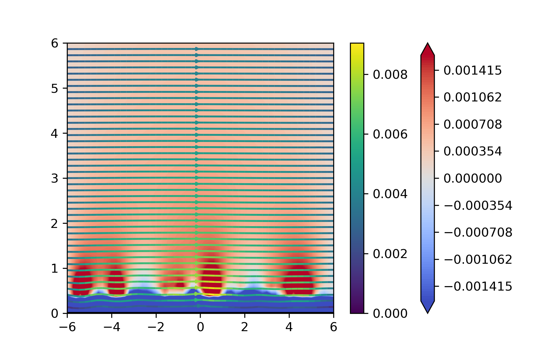
(a) $t=0.05$

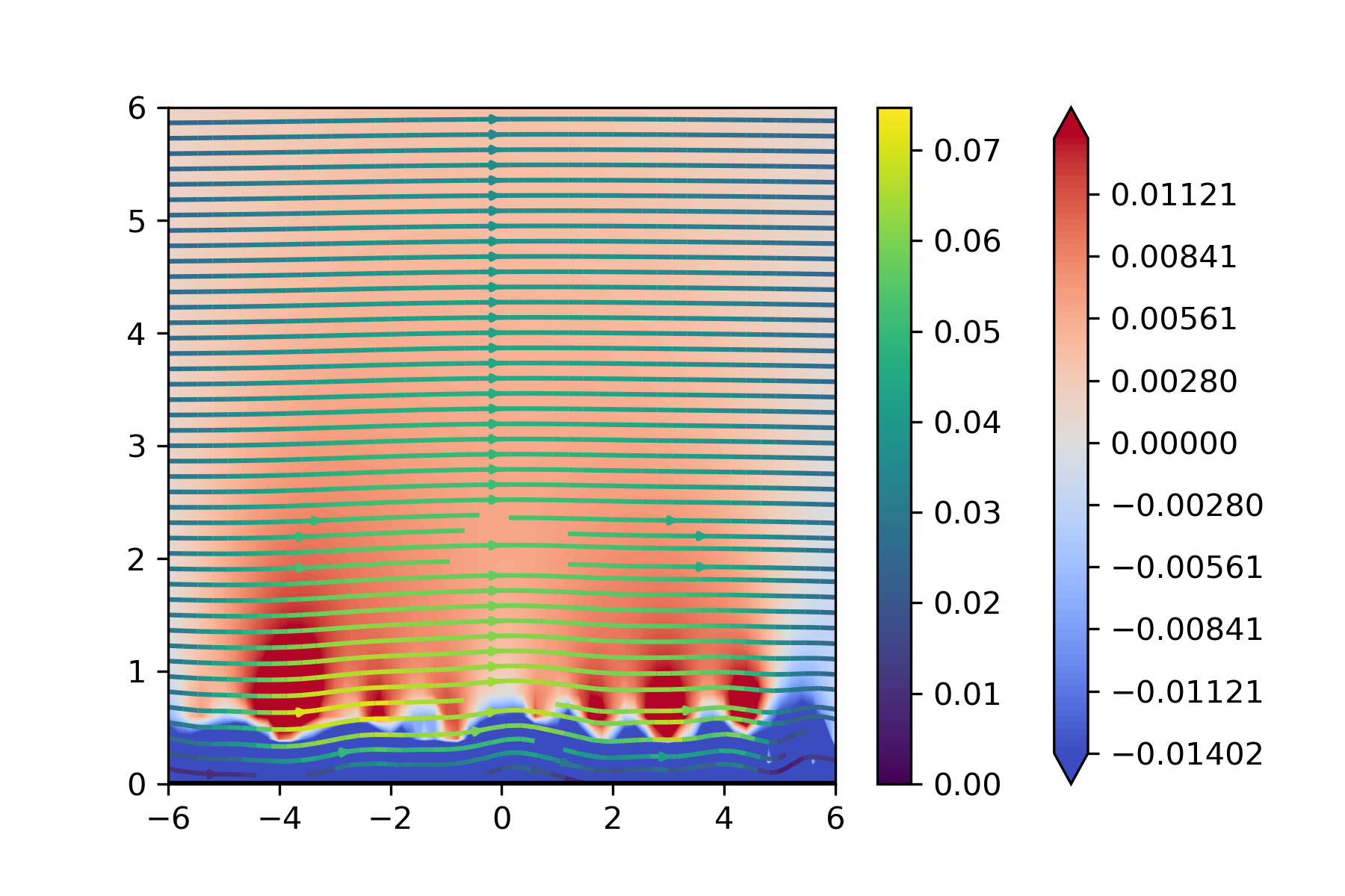
(b) $t=0.25$

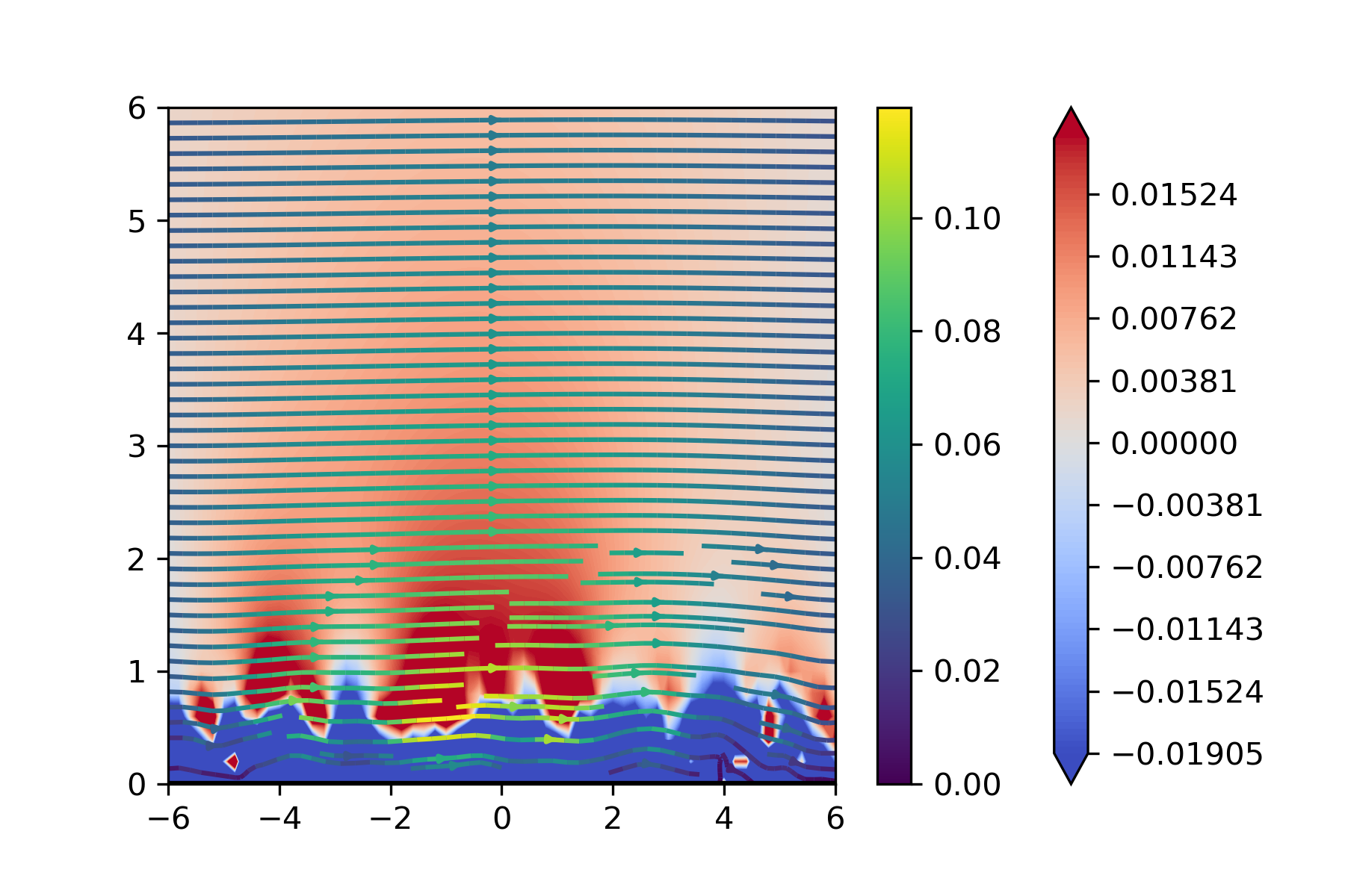
(c) $t=0.5$

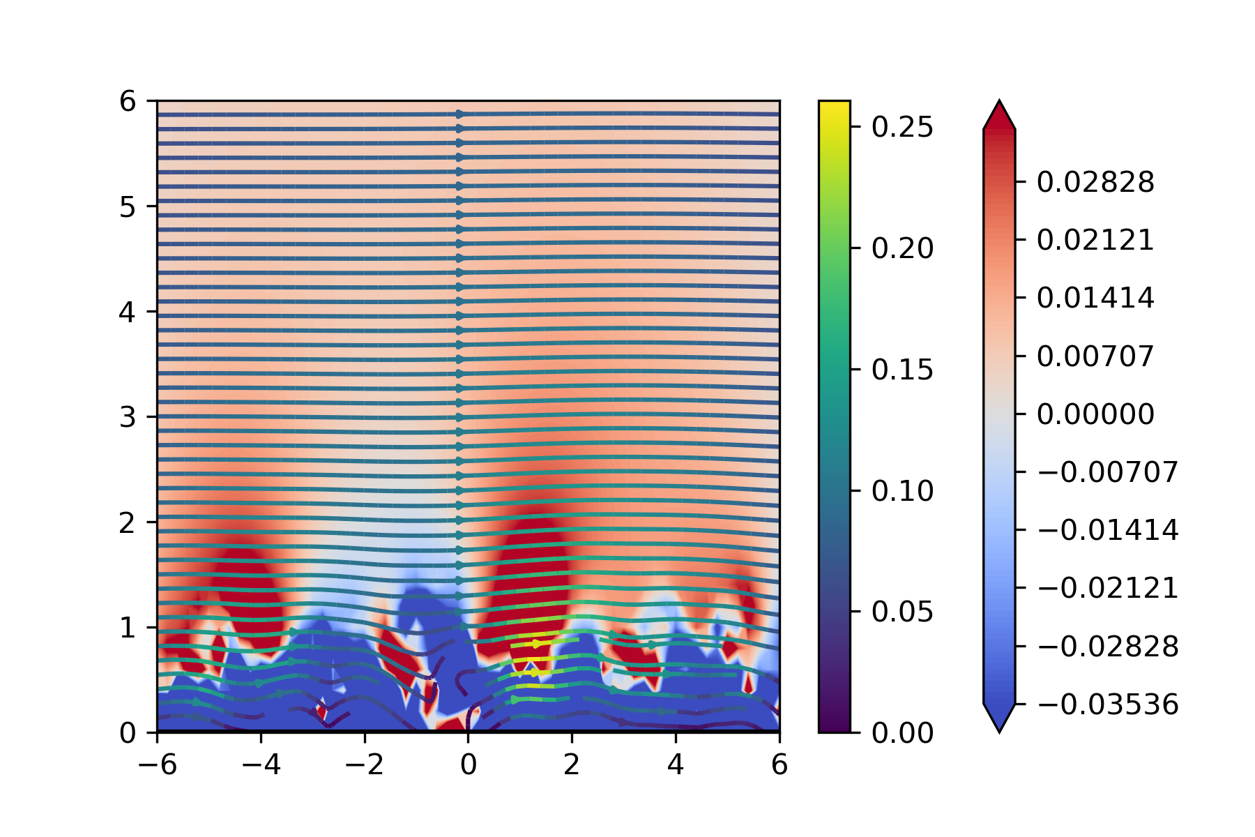
(d) $t=1.0$

Figure 5.1: The outer layer flow at different times $t$.

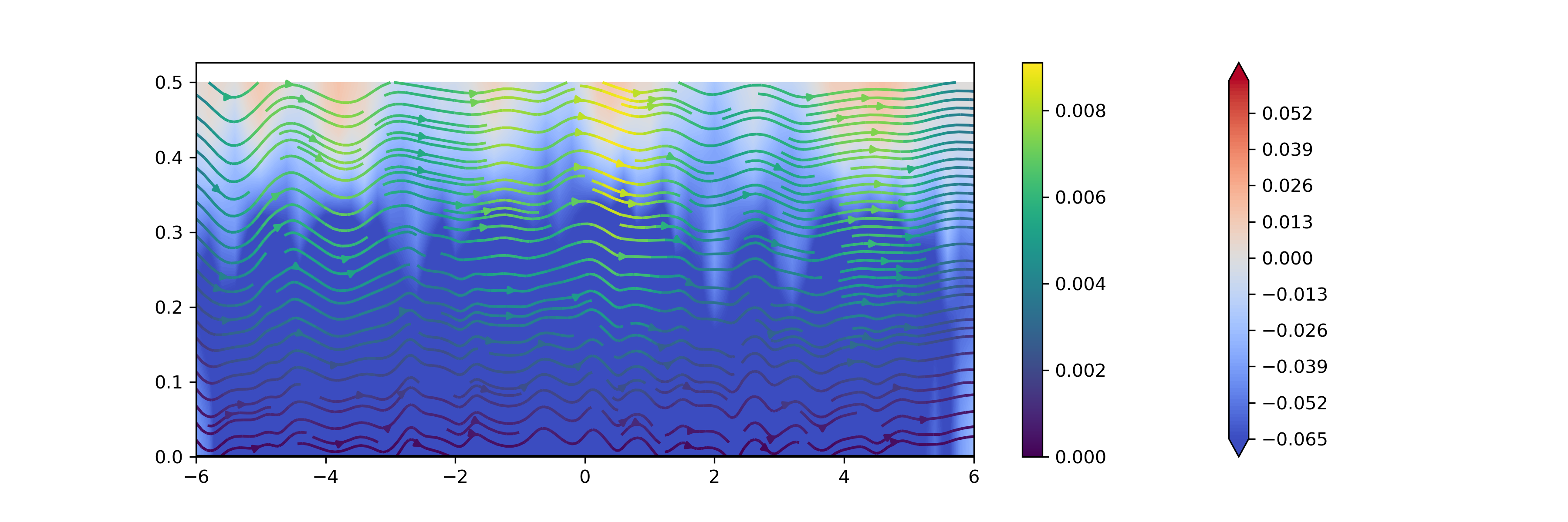
(a) $t=0.05$

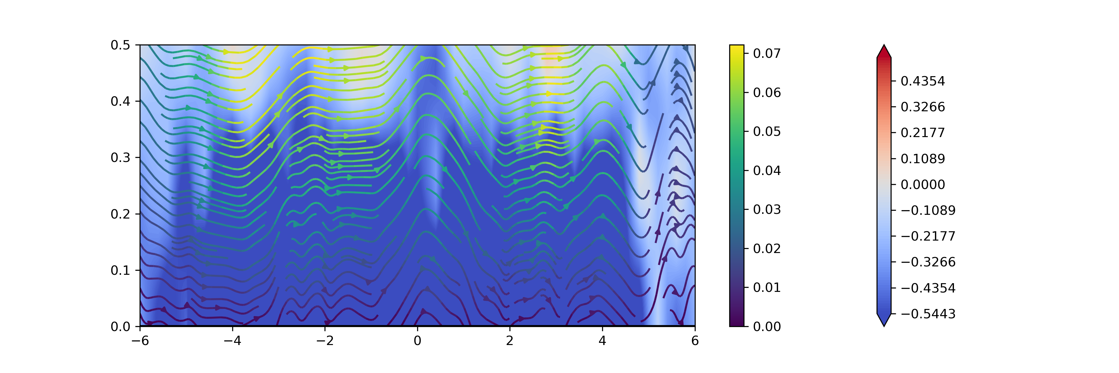
(b) $t=0.25$

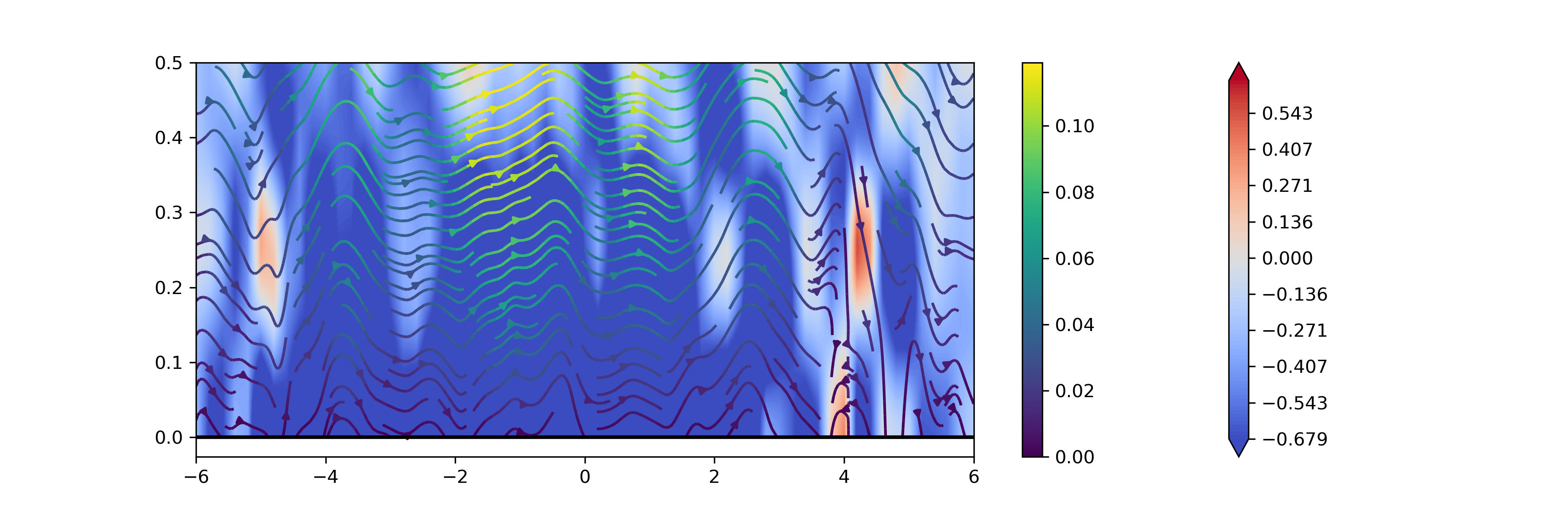
(c) $t=0.5$

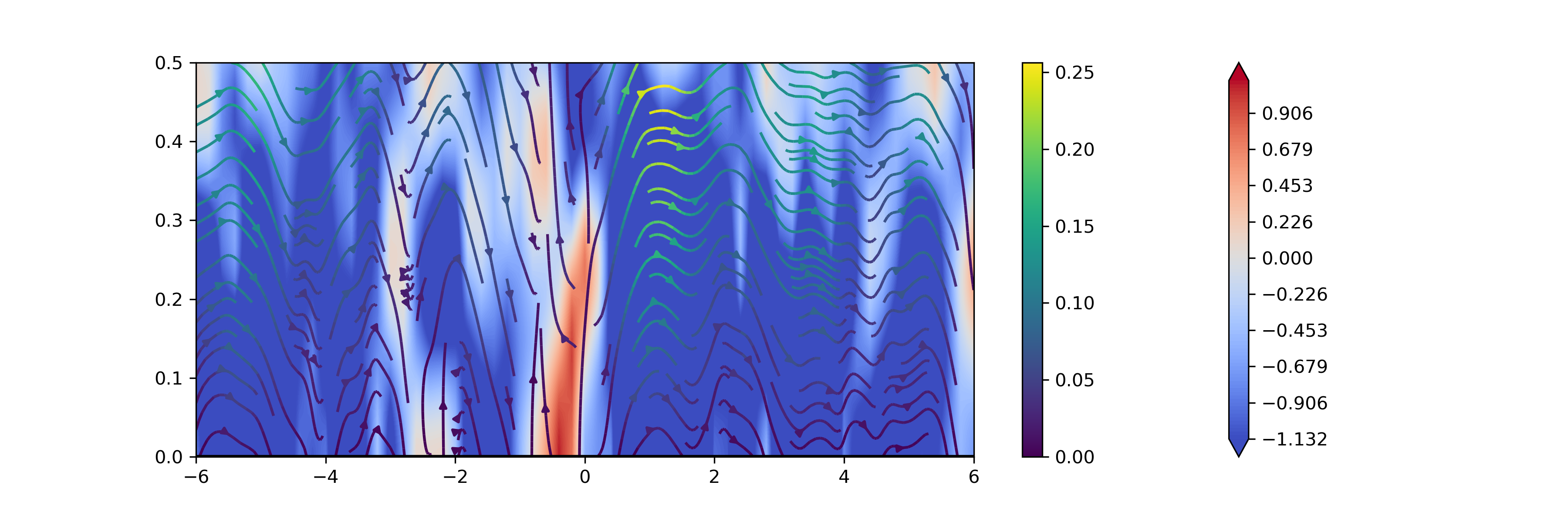
(d) $t=1.0$

Figure 5.2: The boundary layer flow at different times $t$.

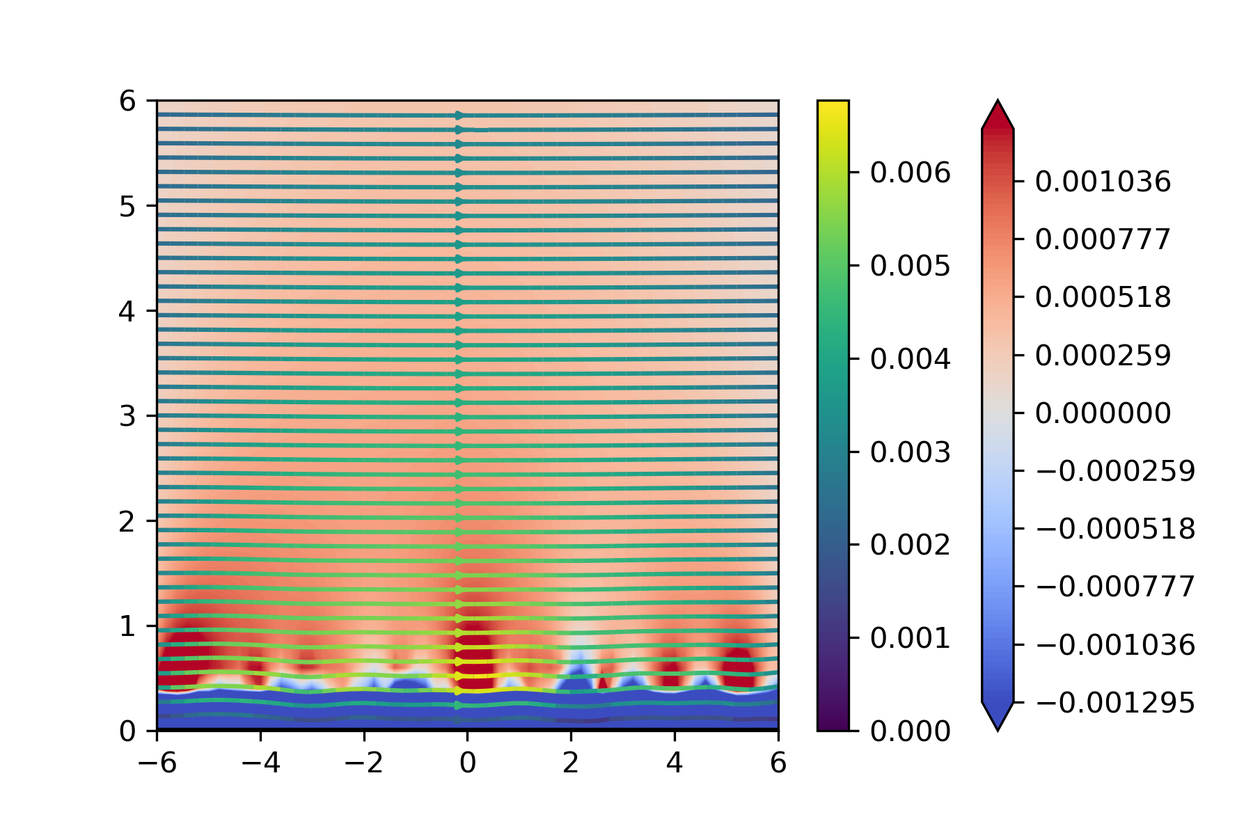
(a) $t=0.05$

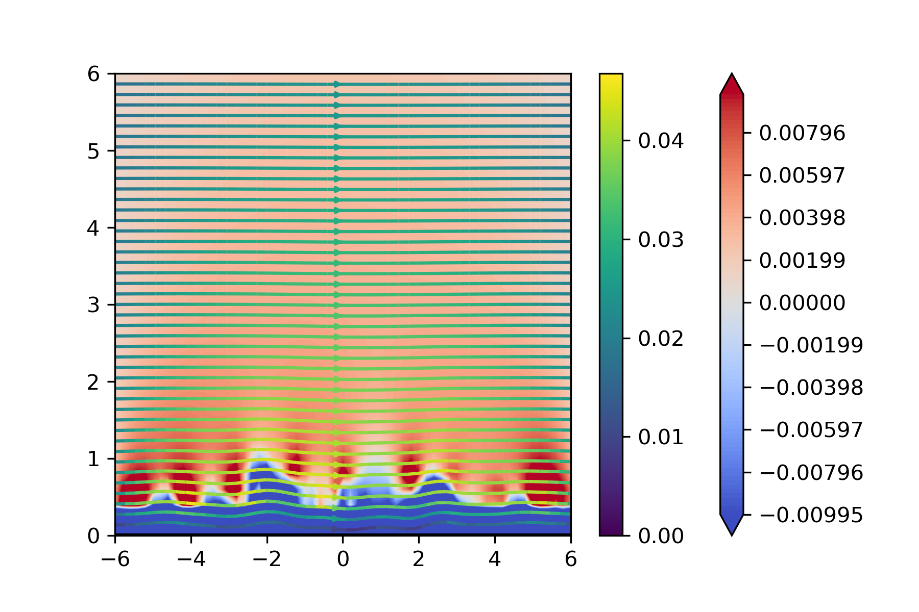
(b) $t=0.25$

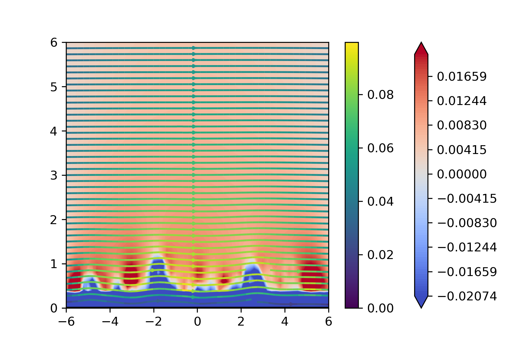
(c) $t=0.5$

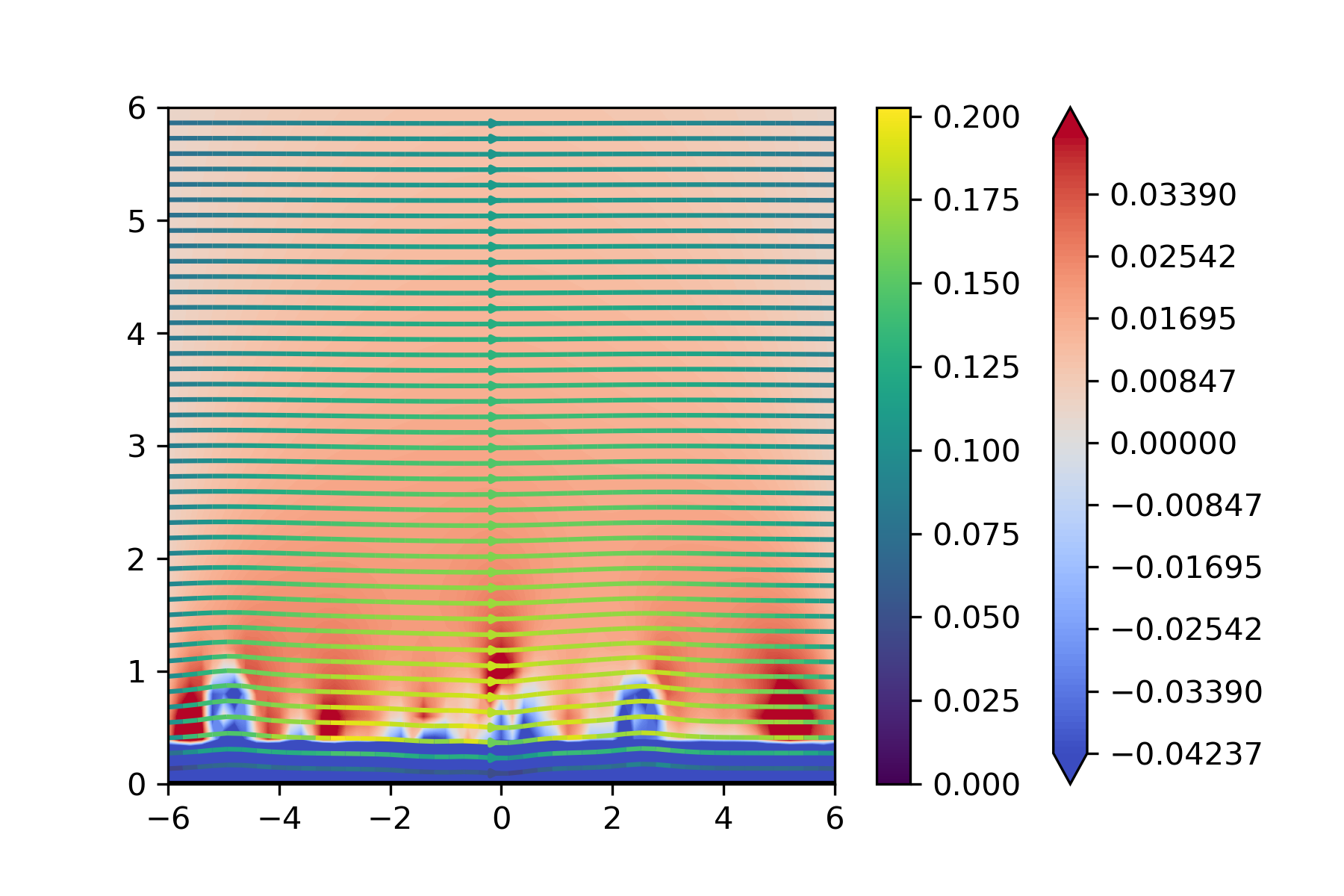
(d) $t=1.0$

Figure 5.3: The outer layer flow at different times $t$.

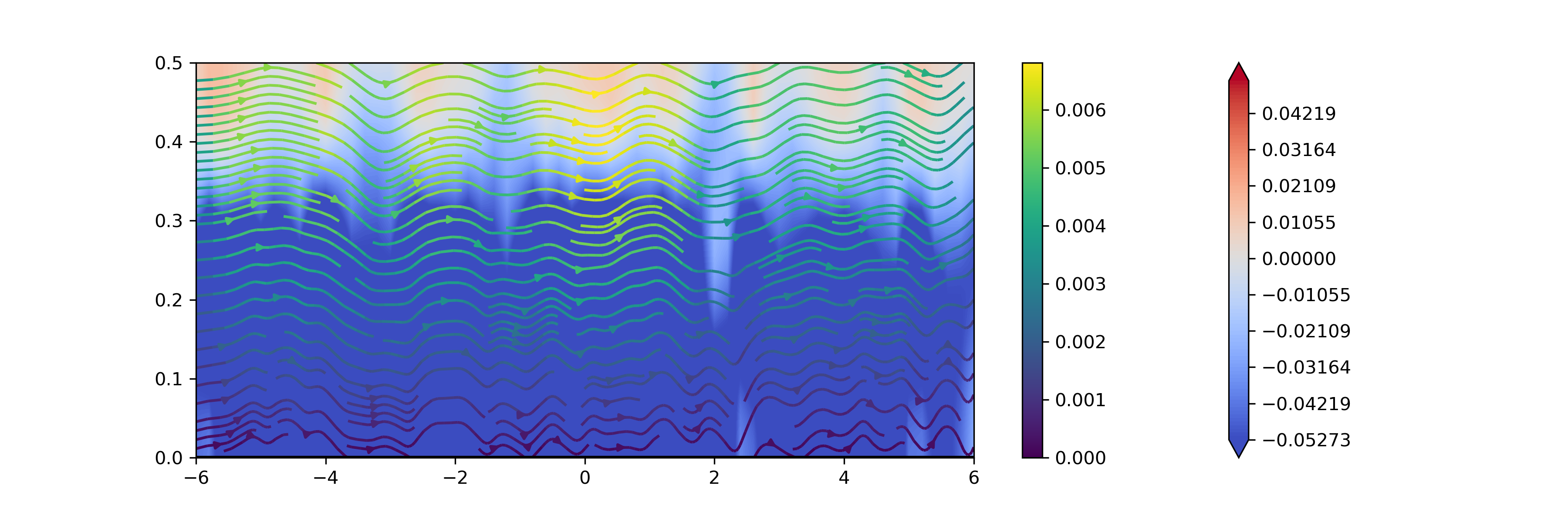
(a) $t=0.05$

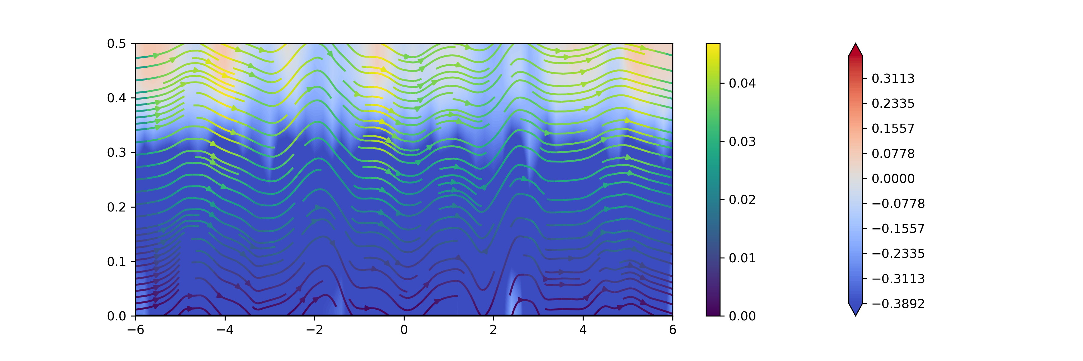
(b) $t=0.25$

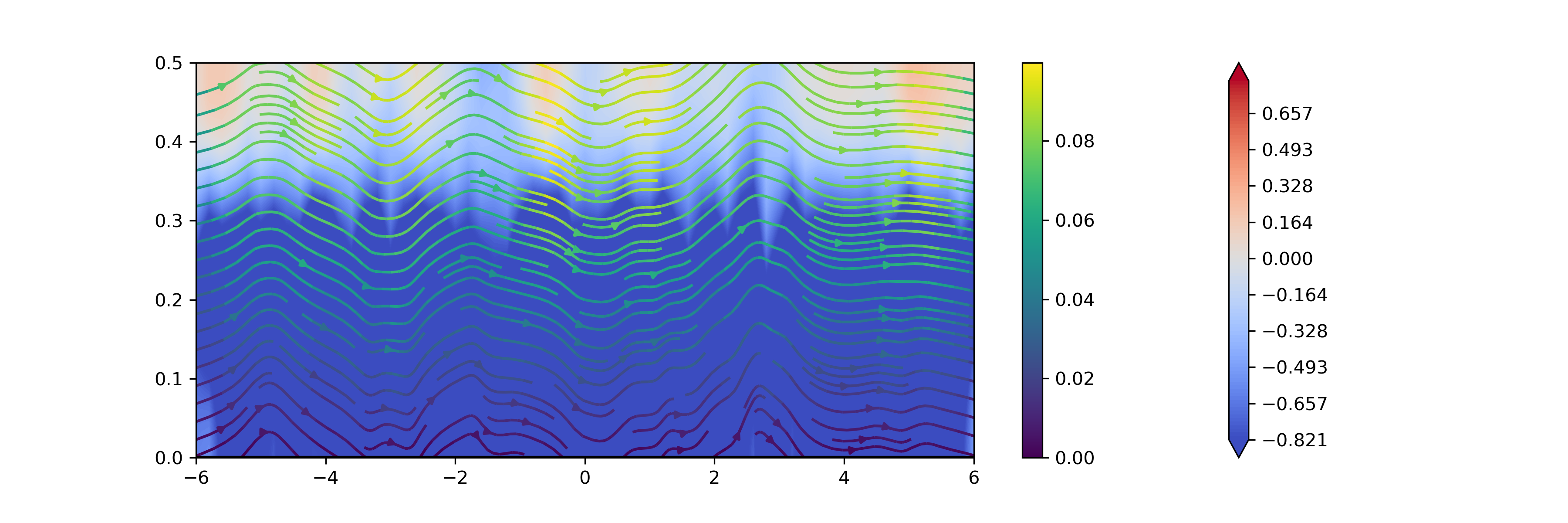
(c) $t=0.5$

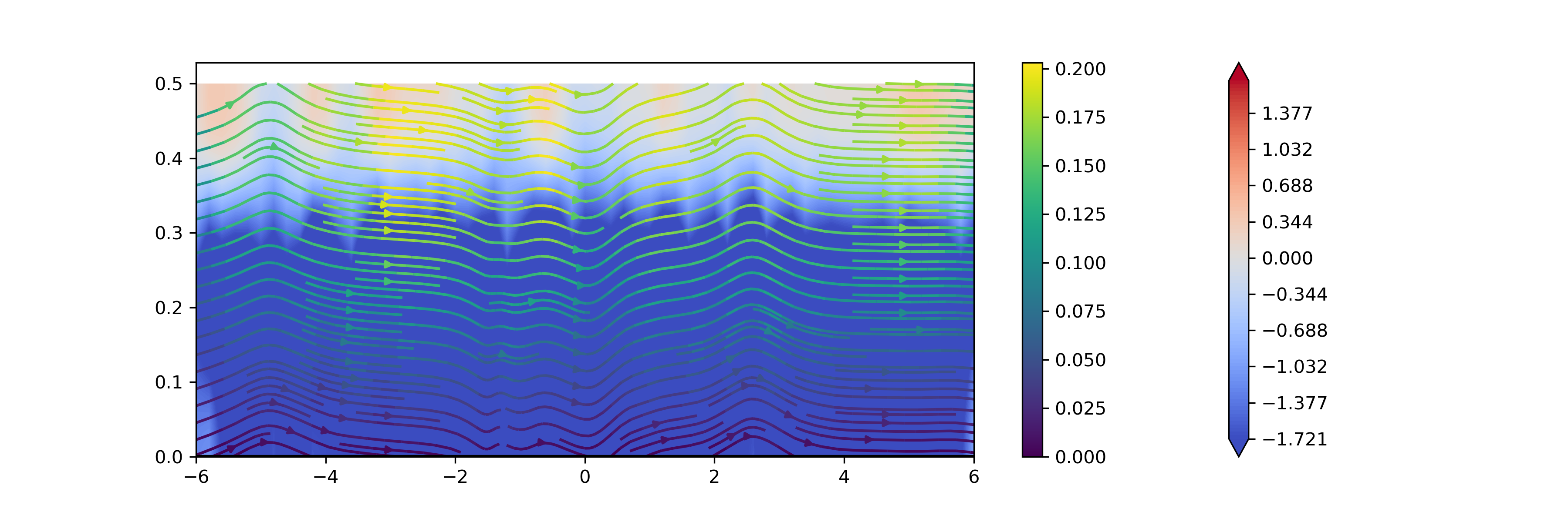
(d) $t=1.0$

Figure 5.4: The boundary layer flow at different times $t$.

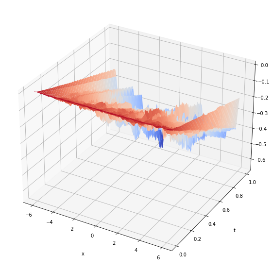
(a) Boundary vorticity $\theta(x_{1},t)$

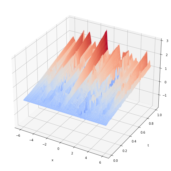
(b) Third order derivative term $\nu\frac{\partial^{3}u^{1}}{\partial x_{2}^{3}}(x_{1},t)$

Figure 5.5: The boundary vorticity $\theta$ and the $\nu\frac{\partial^{3}u^{1}}{\partial x_{2}^{3}}$ as functions of position at boundary $x_{1}$ and time $t$.

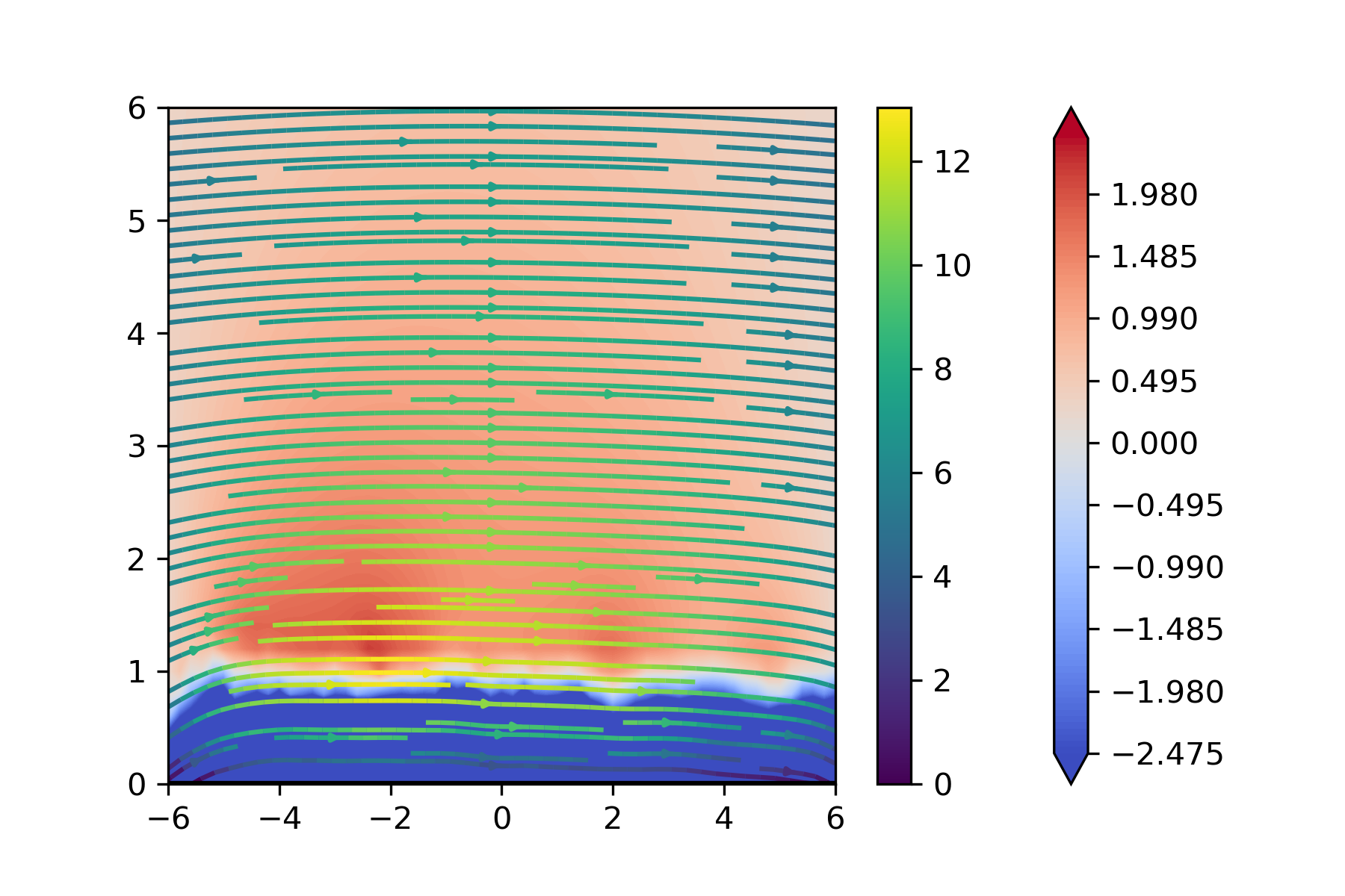
(a) $t=0.15$

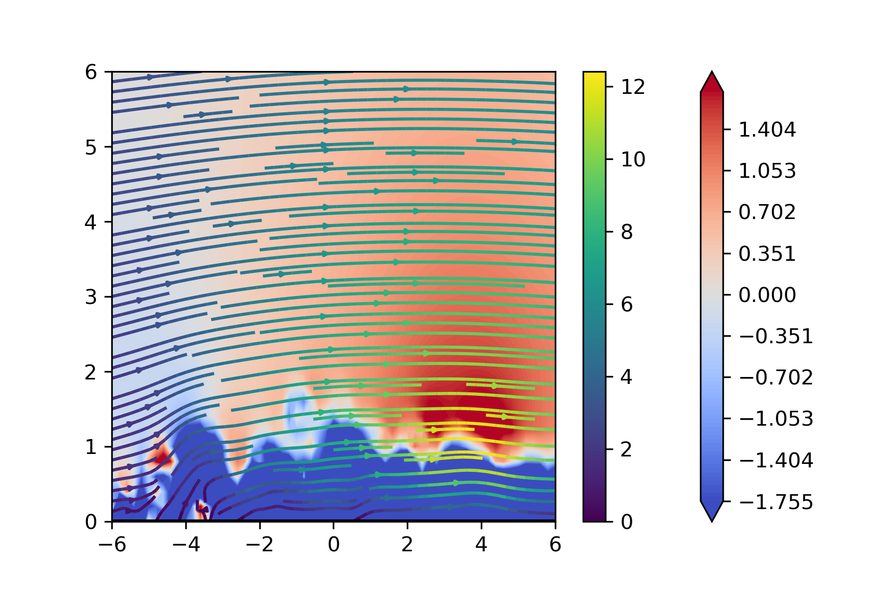
(b) $t=0.75$

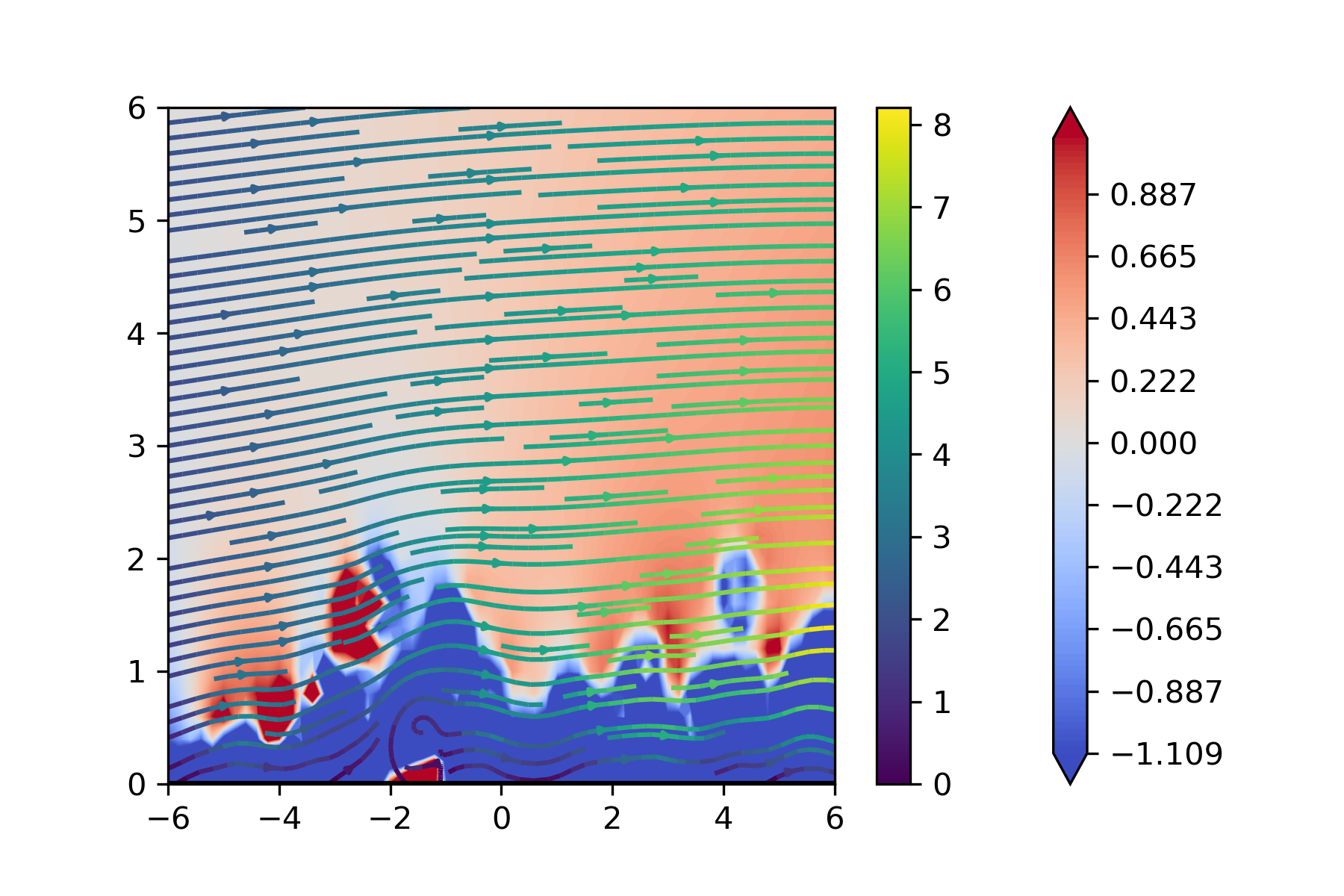
(c) $t=1.5$

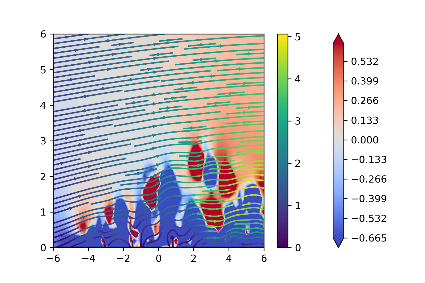
(d) $t=3.0$

Figure 5.6: The outer layer flow at different times $t$.

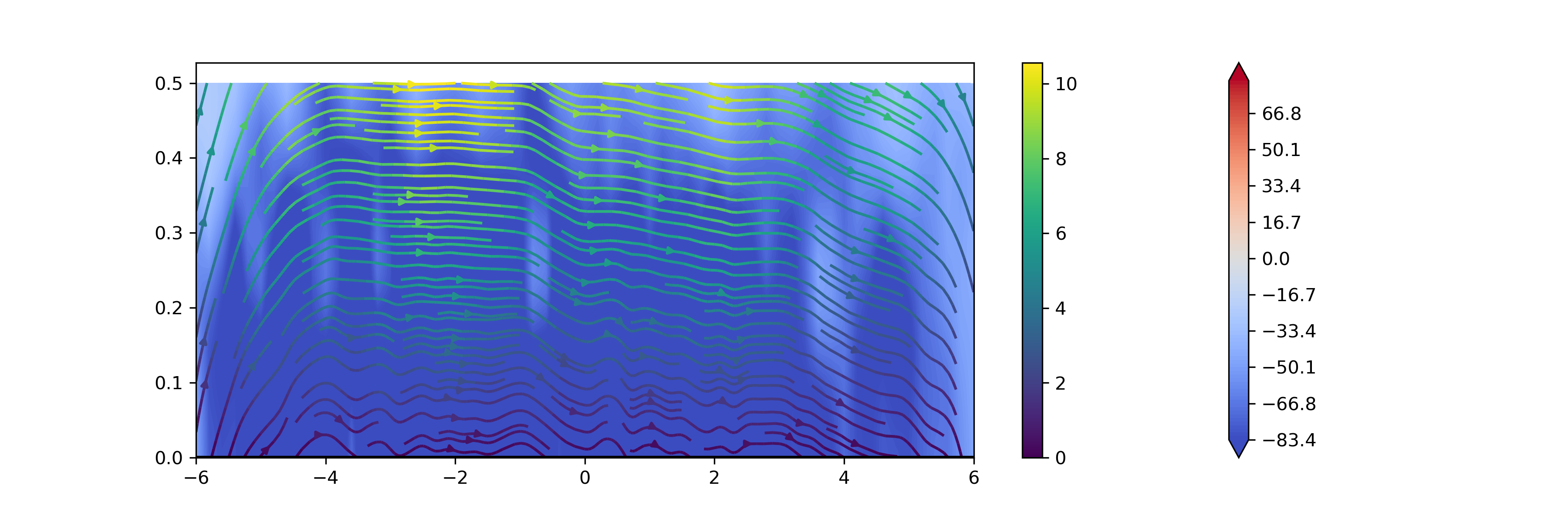
(a) $t=0.15$

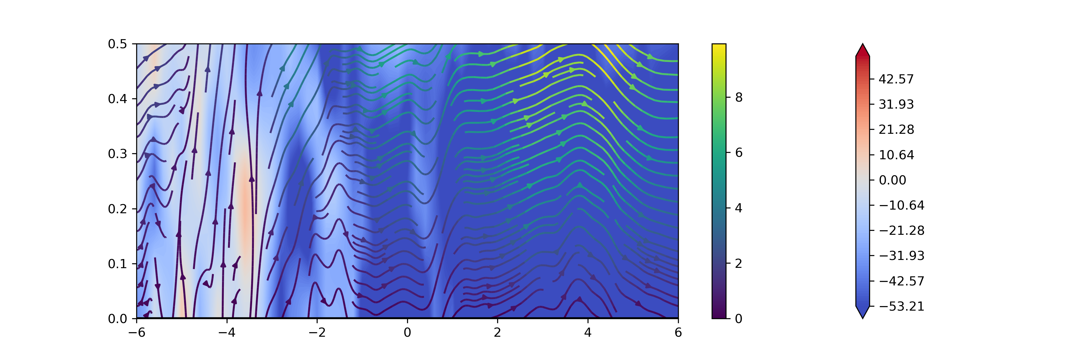
(b) $t=0.75$

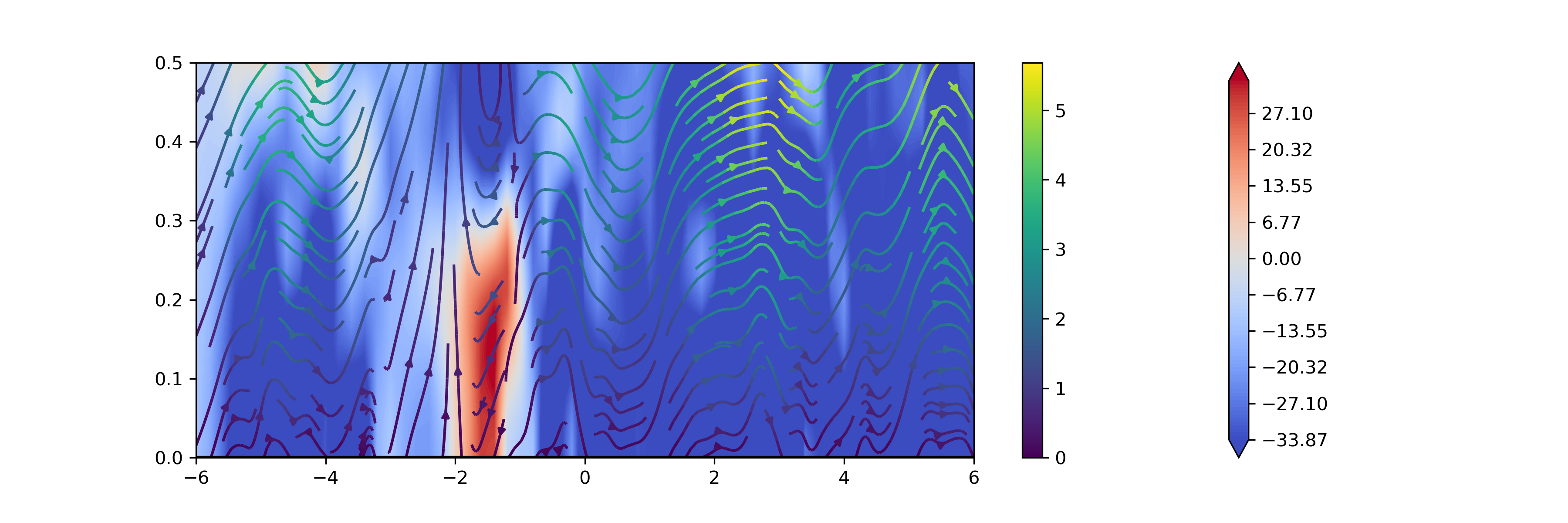
(c) $t=1.5$

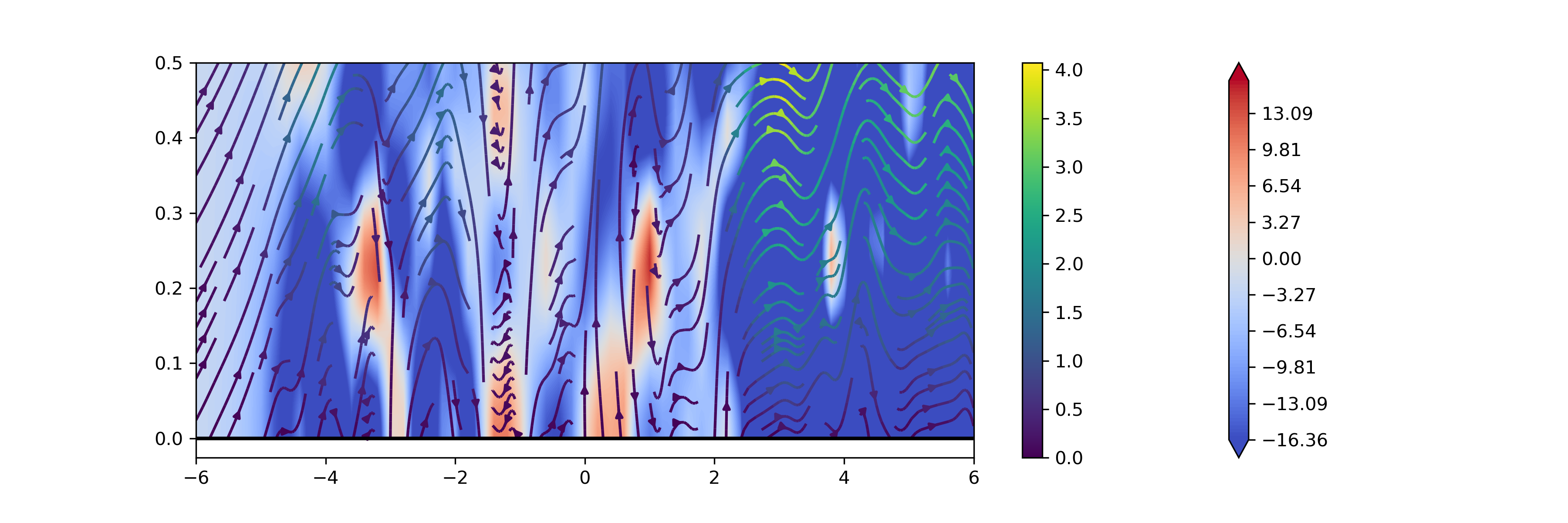
(d) $t=3.0$

Figure 5.7: The boundary layer flow at different times $t$.

Data Availability Statement

The data that support the findings of this study are available from the corresponding author upon reasonable request.

References

• [1] Anderson, C. and Greengard, C. 1985 On vortex methods. SIAM J. Numer. Anal. $\mathbf{22}$ (3), 413-440.
• [2] Cherepanov, V. and Qian, Z. 2023 Monte-Carlo method for incompressible fluid flows past obstacles. arXiv:2304.09152
• [3] Chorin, A. J. 1973 Numerical study of slightly viscous flow. J. Fluid Mech. $\mathbf{57}$, 785-796.
• [4] Cottet, G. -H., and Koumoutsakos, P. D. 2000 Vortex methods: theory and practice. Cambridge University Press.
• [5] Goodman, J. 1987 Convergence of the random vortex method. Comm. Pure Appl. Math. $\mathbf{40}$(2), 189-220.
• [6] Leonard, A. 1980 Vortex methods for flow simulation, Journal of Computational Physics, 1980, Pages 289-335.
• [7] Li, J., Qian, Z. and Xu, M. 2023 Twin Brownian particle method for the study of Oberbeck-Boussinesq fluid flows. arXiv:2303.17260
• [8] Majda, A. J. and Bertozzi A. L. 2002 Vorticity and incompressible flow. Cambridge University Press.
• [9] Marchioro, C. and M. Pulvirenti 1984 Vortex methods in two-dimensional fluid dynamics, Springer.
• [10] Qian Z. 2022 Stochastic formulation of incompressible fluid flows in wall-bounded regions. arXiv:2206.05198
• [11] Qian, Z., Qiu, Y., Zhao, L. and Wu, J. 2022 Monte-Carlo simulations for wall-bounded fluid flows via random vortex method. arXiv:2208.13233