Using Photometrically-Derived Properties of Young Stars to Refine TESS’s Transiting Young Planet Survey Completeness

Abstract

The demographics of young exoplanets can shed light onto their formation and evolution processes. Exoplanet properties are derived from the properties of their host stars. As such, it is important to accurately characterize the host stars since any systematic biases in their derivation can negatively impact the derivation of planetary properties. Here, we present a uniform catalog of photometrically-derived stellar effective temperatures, luminosities, radii, and masses for 4,865 young ($<$1 Gyr) stars in 31 nearby clusters and moving groups within 200 pc. We compared our photometrically-derived properties to a subset of those derived from spectra, and found them to be in good agreement. We also investigated the effect of stellar properties on the detection efficiency of transiting short-period young planets with TESS as calculated in Fernandes et al. (2022), and found an overall increase in the detection efficiency when the new photometrically derived properties were taken into account. Most notably, there is a $1.5\times$ increase in the detection efficiencies for sub-Neptunes/Neptunes (1.8–6 $R_{\oplus}$) implying that, for our sample of young stars, better characterization of host star properties can lead to the recovery of more small transiting planets. Our homogeneously derived catalog of updated stellar properties, along with a larger unbiased stellar sample and more detections of young planets, will be a crucial input to the accurate estimation of the occurrence rates of young short-period planets.

1 Introduction

The discovery of thousands of transiting exoplanets via large-scale surveys such as Kepler (Borucki et al., 2010), K2 (Howell et al., 2014), and TESS (Ricker et al., 2014) has enabled us to explore not only individual planets and systems, but also planet populations. However, the determination of exoplanet properties are dependent on robust knowledge of their host stars, most notably stellar radii, masses, and effective temperatures which can be used to derive planet radii, masses, and equilibrium temperatures. In order to facilitate target selection, catalogs providing basic stellar properties were developed for Kepler, K2, and TESS such as the Kepler Input Catalog (KIC, Brown et al., 2011), the Ecliptic Plane Input Catalog (EPIC, Huber et al., 2016), and the TESS Input Catalog (TIC, Stassun et al., 2018), respectively. These input catalogs were derived by combining data from heterogeneous sources, and hence cannot be used as a precise reference for stellar properties and exoplanet demographics.

For studies of exoplanet populations, it is especially crucial to have a homogeneously derived stellar catalog as any systematic biases in the derivation of the stellar properties can negatively impact the derivation of planetary properties, and therefore lead to the incorrect characterization of the planet populations. One prominent example is the discovery of the radius valley in Kepler’s short-period small planet population, which was enabled by uniform spectroscopic (Fulton et al., 2017) and astroseismic (Van Eylen et al., 2018) stellar classification. The Gaia mission (Gaia Collaboration et al., 2016) has transformed the field of stellar classification, providing photometry and distances to over a billion stars (Gaia Collaboration et al., 2018, 2021). With Gaia DR2 data, Berger et al. (2020) and Hardegree-Ullman et al. (2020) were able to update the Kepler and K2 stellar catalogs, respectively, in a homogeneous manner, with the latter enabling the confirmation of the planet radius valley beyond the Kepler field. Stassun et al. (2019) also incorporated Gaia DR2 data into the TIC. However, there are still many inhomogeneities in the derivation of TIC stellar properties, so it should not be used for large-scale exoplanet demographic studies. A fully uniform catalog of TESS stellar properties for nearly two billion stars is a difficult task, but uniform catalogs of subsets of TESS targets are a much more tractable goal.

While most known short-period transiting exoplanets have been found orbiting Gyr-old stars, over the past decade K2 and TESS have facilitated the discovery of $>$30 young ($<$1 Gyr) exoplanets (A. Vanderburg priv. comm.; e.g., Newton et al., 2019, 2021; Rizzuto et al., 2020; Mann et al., 2020; Nardiello et al., 2020; Bouma et al., 2020). The discovery and characterization of young short-period exoplanets is crucial to our understanding of planet formation and evolution processes such as photoevaporation (e.g., Owen & Wu, 2013, 2017), and core-powered mass loss (e.g., Ginzburg et al., 2016, 2018; Gupta & Schlichting, 2019, 2020, 2020). Young stellar clusters and moving groups are promising targets to search for such planets. TESS enables this search by providing light curves spanning nearly the entire sky. However, if we hope to learn about the demographics of young planets, we still need a uniform catalog of stellar properties. Young stars are typically still evolving onto the main sequence, so their properties cannot necessarily be derived using the same assumptions, inputs, or relationships as their main sequence counterparts. While past studies of individual young clusters and associations have yielded stellar properties for those clusters (e.g., Fang et al., 2023), we aim to study planets in all known nearby young clusters and associations (within 200 pc), and this necessitates a larger homogeneous catalog.

Ideally, we would have a spectrum for each star to yield precise spectral type, effective temperature, surface gravity, and metallicity information. However, less than 10% of our sample of young stars have spectra and so we must depend on available photometry to characterize these stars. Here, we present a uniformly derived catalog of photometrically-derived stellar properties for 4,865 stars in nearby (within 200 pc) young clusters and moving groups. In Section 2, we used data from Gaia DR3 to derive stellar effective temperatures, luminosities, radii, and masses. We tested our derived stellar properties by comparing them to properties measured from spectra for a subset of our sample in Section 3. Next, we used our stellar catalog to update the detection efficiency analysis and planet occurrence rate calculations for young stars from Fernandes et al. (2022) in Section 4. Finally, we summarized our results and discuss the next steps needed to further improve our stellar catalog and planet occurrence rates for young stars in Section 5.

2 Stellar Classification

The focus of this work is to compute a homogeneous catalog of stellar $T_{\text{eff}}$, radii, and masses to aid in the accurate estimation of young transiting exoplanet radii as well as to place constraints on their demographics. Given that TESS decreases in sensitivity to transiting planets orbiting fainter low-mass stars (e.g., Dietrich et al., 2023), we only classified stars of F, G, K, and early M spectral types (down to M3.5 V) as they are typically bright enough and have a higher chance of hosting a detectable planet with TESS.

Our sample of nearby moving groups and young clusters was compiled using the BANYAN $\Sigma$ (Gagné et al., 2018), and the Gaia DR2 open cluster member lists (Gaia Collaboration, Babusiaux et al. 2018). We also added the more recently discovered Argus (Zuckerman, 2019), MUTA (Gagné et al., 2020), and Pisces-Eridanus (Curtis et al., 2019) groups. We restricted the median moving group or young cluster distance to $\sim$200 pc to ensure that we can detect planets around later K- and early M-type stars with TESS. We excluded clusters younger than 10 Myr since their stars could still retain a disk (e.g., Ercolano & Pascucci, 2017), and their light curves are highly complex and variable (e.g., Cody et al., 2014). We included clusters up to 1 Gyr to cover ages over which the short-period planet population is expected to evolve (e.g., Rogers et al., 2021). With these distance and age cuts, we obtained a starting sample of 10,585 young stars from 31 young clusters and moving groups (see Table 3 in Appendix A).

2.1 Main Sequence vs. Pre-Main Sequence Sample

The age at which any given star reaches the main sequence depends on its stellar mass: a 1.6 $M_{\odot}$ F-type star takes $\sim$20 Myr to reach the main sequence, whereas a 0.1 $M_{\odot}$ M dwarf (like TRAPPIST-1) can take up to one billion years. However, the majority of our sample of young stars do not have measured masses, which makes it challenging to determine which stars in a given cluster are pre-main sequence and which stars have already reached the main sequence. To combat this, we relied on $G$, $G_{BP}$, and $G_{RP}$ band magnitudes for our targets from Gaia DR3 (Gaia Collaboration et al., 2022b), along with distances from Bailer-Jones et al. (2021), and 2MASS IDs and photometry (Skrutskie et al., 2006) from Gaia’s best neighbour cross-match (see Table 3 in Appendix A). At this stage, we removed all targets with non-finite magnitudes, parallaxes, and associated errors since we could not compute stellar properties for them, leaving us with 10,238 targets.

In crowded fields (typical in young cluster environments), it is highly probable that a given exoplanet transit is diluted due to the light from a bound companion star which can lead to an underestimated planet radius measurement. To this effect, we identified and removed any known binaries and non-single sources in our sample using the Gaia EDR3 binary catalog (El-Badry et al., 2021), the Robo-AO census of companions within 25 pc (Salama et al., 2022), and the Gaia DR3 non-single stars catalog (Gaia Collaboration et al., 2022a), leaving us with 9,462 targets. Gaia also provides a Renormalised Unit Weight Error (RUWE) score for each source. For sources where the astrometric observations fit well with the single-star model, the expected RUWE value is around 1.0. However, a value greater than 1.0 suggests the source could be either non-single or has other issues that may affect the accuracy of the astrometric solution. Targets with a RUWE score $>1.4$ have been found to be indicative of a non-single source (Ziegler et al., 2020). As such, we also removed any stars with a Gaia DR3 RUWE score $>1.4$, which left us with 8,239 stars for which stellar properties could be computed.

Here, it is important to note that although we removed all known binaries and sources with high RUWE scores from our sample, there is still a possibility of unresolved binaries leading to improper star classification. For instance, if a G-type main sequence star has an unresolved equal-mass binary, the photometric colors would not be affected, but the combined flux from both stars would lead to an overestimation of the system’s luminosity. This overestimation of the luminosity would propagate into the mass and radius estimates derived from the luminosity, leading to an overestimation of both quantities. Since pre-main sequence stars are more luminous and have larger radii, the mischaracterization of a main sequence star as pre-main sequence could occur if there is an unresolved binary. This mischaraterization would further propagate into the derivation of the planet radii. More specifically, an equal mass binary would cause the luminosity to be overestimated by 2$\times$. This means that the radius of the star as derived from the flux would be $\sqrt{2}\times$ larger than the true radius. This would cause the transit depth of the planet to be diluted by 0.5$\times$, and the radius of the planet to be underestimated by $\sqrt{2}\times$ or approximately 41.42%. Assuming a stellar multiplicity rate of 44% and 26% for FGK and M stars respectively (Duchêne & Kraus, 2013), and given that our previous known binary and high RUWE score cuts removed $\sim$20% of the sample, we are left with a possible $\sim$292 to 1,168 unresolved binaries in our sample that are likely mischaracterized. Dilution resulting from unresolved binaries is also expected to hinder our ability to detect the transit signals of smaller planets, ultimately reducing our detection efficiency within those particular bins. To address this issue, performing a thorough assessment of the multiplicity of each star in our sample would be ideal. However, it would necessitate extensive ground-based follow-up using high-resolution imaging, which is beyond the scope of this paper.

Using the intrinsic color of a star i.e., the difference in magnitude calculated using two different color filters, along with the absolute magnitude, we created a Hertzsprung-Russell diagram (Hertzsprung, 1911; Russell, 1914) to differentiate between the pre-main sequence and main sequence stars (see Figure 1).

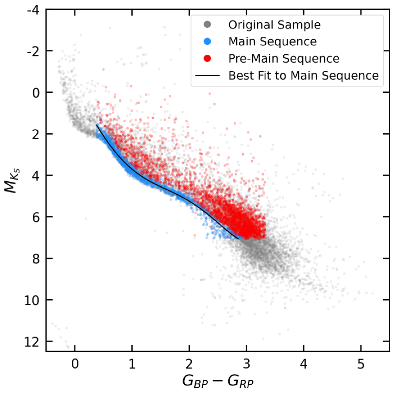
Figure 1: Hertzsprung-Russell diagram of our starting sample of stars from 31 young clusters and moving groups (grey). Stars classified in this work as pre-main sequence and main sequence stars are also shown in red and blue, respectively. Around $M_{K_{S}}$=2 mag there is an apparent bifurcation in the main sequence stars. The sparsity of data points in that region for which to fit our color-magnitude polynomial could lead to some misclassification of pre-main sequence stars as main sequence stars, which we think is happening here.

Here, we used Gaia DR3 and 2MASS photometry of the standard main-sequence stars that were used to create Table 5 from Pecaut & Mamajek (2013, henceforth PM13) in order to establish $M_{K_{S}}$ vs. $G_{BP}-G_{RP}$ or $G-G_{RP}$ relationships. We determined the main sequence by fitting a 5^th order polynomial to $M_{K_{S}}$ and $G_{BP}-G_{RP}$. The polynomial order for each of the fits in this paper was the lowest order needed to fit large-scale structure while higher orders did not significantly improve the RMS residual scatter. Since $G_{BP}$ is not well constrained for intrinsically redder stars, we instead fit $M_{K_{S}}$ and $G-G_{RP}$ with a 5^th order polynomial for targets with $4.5<M_{K_{S}}<10$. All stars within 10% of both these fits were analyzed as main-sequence stars in this work, while the rest were analyzed as pre-main sequence i.e. stars of a given color are labeled as main sequence if their magnitude is within 10% of that found by evaluating the main sequence best-fit polynomial at that color. At this point, we also removed stellar populations that we could not accurately classify for both main sequence and pre-main sequence populations: white dwarfs and OBA stars ($0.5<G_{BP}-G_{RP}<3.5$), and late M stars ($M_{K_{S}}>7.1$). These cuts gave us a total population of 4,865 stars (1,824 main sequence, and 3,041 pre-main sequence) for which we derived stellar properties (see Figure 1).

2.2 Stellar Effective Temperatures and Radii

Using intrinsic colors, we can derive stellar effective temperature (hereafter, $T_{\text{eff}}$). The $T_{\text{eff}}$ for pre-main sequence stars was computed by fitting a 7^th degree polynomial to the derived $G_{BP}-G_{RP}$ colors and $T_{\text{eff}}$ for pre-main sequence stars from PM13 Table 6. We note that the PM13 pre-main sequence table does not have Gaia color information, but it has $V-I_{c}$ colors, which we converted to $G_{BP}-G_{RP}$ using Gaia photometric relations with other photometric catalogs (Busso et al., 2021). For main sequence stars, we fit a 4^th order polynomial to $G_{BP}-G_{RP}$ versus $T_{\text{eff}}$ from the set of individual measurements from standard stars used to create the most recent version of the PM13 Table 5.

All uncertainties herein were calculated using a Monte Carlo method. For $T_{\text{eff}}$, we started with each $G_{BP}$ and $G_{RP}$ magnitude and associated error, drew a normal distribution of 1000 points, computed $G_{BP}-G_{RP}$ from those posteriors, ran the $G_{BP}-G_{RP}$ posterior through the polynomial fit, and took the median value of the resultant distribution as our $T_{\text{eff}}$. We added the standard deviation of the $T_{\text{eff}}$ distribution in quadrature to the $\sim$1% and $\sim$1.66% rms deviation from the polynomial fits for pre-main main sequence stars, respectively. The median uncertainties on $T_{\text{eff}}$ are 1.34% and 2.67% for pre-main and main sequence stars, respectively. The main sequence $T_{\text{eff}}$ uncertainties are larger because there were significantly more data points used for that polynomial fit, resulting in a larger rms scatter. Our $T_{\text{eff}}$ uncertainties are likely underestimated, but they are the best we can do given the data we have for our polynomial fits. We urge caution using these $T_{\text{eff}}$ uncertainties for individual targets.

In Section 2.1, we used $M_{K_{S}}$ magnitudes to define our sample of main and pre-main sequence stars, particularly to help establish cutoffs for late M dwarfs. Since we are classifying stars from F to early M, we chose to apply bolometric corrections in the optical $G$ band to minimize these corrections across different spectral types. We calculated the bolometric magnitude using the absolute $G$ magnitude ($M_{\text{G}}$), the bolometric correction in $G$ band ($BC_{\text{G}}$), and the total extinction in $G$ band ($A_{\text{G}}$) as in the equation below:

$$M_{\text{bol}}=M_{\text{G}}+BC_{\text{G}}-A_{\text{G}}$$ (1)

Since we did not immediately have a value for $BC_{\text{G}}$, we converted PM13’s $BC_{\text{J}}$ to $BC_{\text{G}}$. We first fit a 7^th degree polynomial to the $G_{BP}-G_{RP}$ colors we computed earlier and $BC_{\text{J}}$ from PM13 Table 6 and used that relation to compute $BC_{\text{J}}$ for our targets. Then we converted $BC_{\text{J}}$ to $BC_{\text{G}}$ with $BC_{\text{G}}$ $=BC_{\text{J}}-(m_{G}-m_{J})$, where $m_{G}$ and $m_{J}$ are the apparent magnitudes in Gaia G and 2MASS J bands, respectively. We then computed the bolometric luminosity as follows:

$$L_{\text{bol}}=L_{\text{0}}\times 10^{-0.4\times M_{\text{bol}}}$$ (2)

where $L_{0}=3.0128\times 10^{28}$ W is an IAU value also used in Mamajek et al. (2015). We accounted for extinction in each band by computing reddening using the dustmaps code (Green, 2018). For targets north of $-30$^∘ in declination, we used the most recent Bayestar map (Green et al., 2019) to compute reddening in $J$-band and converted it to extinction by multiplying the value by 0.7927 from Table 1 of Green et al. (2019). For targets south of $-30$^∘ in declination, which the Bayestar map does not cover since it was calibrated using data from the northern hemisphere Pan-STARRS survey, we used the recalibrated Schlegel et al. (1998) dust map from Schlafly & Finkbeiner (2011). For these targets we computed $E(B-V)$ using dustmaps and converted it to $A_{V}$ extinction by multiplying the value by 2.742 (assuming $R_{V}=3.1$) from Table 6 of Schlafly & Finkbeiner (2011). We then converted $A_{J}$ and $A_{V}$ to extinction in other bands by multiplying our values by those listed in Table 3 of Wang & Chen (2019), again assuming $R_{V}=3.1$. Since our targets are typically within 200 pc, the effect of extinction is minimal (median $A_{V}=0.03$ mag, $A_{J}=0.007$ mag), so we are not concerned about using two different dust maps for northern and southern targets, or converting extinctions to different bands.

Using our $T_{\text{eff}}$ and luminosity values, we then computed stellar radius using the Stefan-Boltzmann law:

$$R_{\star}=\sqrt[]{\frac{L_{\text{bol}}}{4\pi\sigma_{\text{sb}}T_{\text{eff}}^{4}}}$$ (3)

where $\sigma_{\text{sb}}$ is the Stefan-Boltzmann constant. However, for lower mass or “redder” targets in the range $4.5<M_{K_{S}}<7.1$, the stellar radii were computed using the magnitude–radius relationship from Mann et al. (2015). This magnitude–radius relationship was calibrated using 183 well-characterized nearby K7–M7 single stars and yields radius uncertainties of $\sim$3% for the above $M_{K_{S}}$ magnitude range. FGK stars have higher median radius uncertainties of 3.7% and 5.7% for pre-main and main sequence stars, respectively, but we again urge caution with these uncertainties since they depend partially on our low $T_{\text{eff}}$ uncertainties.

2.3 Stellar Masses

In order to derive stellar masses for the main sequence stars in our sample, we used the mass–luminosity relation from Torres et al. (2010) for stars with $\log(L_{\star}/L_{\odot})>-1$, which corresponds to a mass $M_{\star}\gtrsim 0.7\,M_{\odot}$. Whereas, for targets with $\log(L_{\star}/L_{\odot})<-1$ and in the range $4.5<M_{K_{S}}<7.1$, we computed masses from the empirical magnitude–mass relationship from Mann et al. (2019).

The masses of pre-main sequence stars were derived using stellar evolutionary tracks (e.g., Fang et al., 2021). For this work, we converted the IDL code developed by Pascucci et al. (2016) into Python. This code uses a Bayesian inference approach to estimate stellar mass, age, and associated uncertainties from the stellar $T_{\text{eff}}$, $L_{\text{bol}}$, and a set of isochrones. The conditional likelihood function assumes uniform priors on the model properties and we propagated uncertainties on $T_{\text{eff}}$ and $L_{\text{bol}}$ from our photometric derivations. We used the non-magnetic Feiden (2016) tracks to ages as old as 500 Myr and included new tracks for magnetically-active stars. These new tracks are more appropriate for young M dwarfs ($M_{\star}\lesssim 0.5$ $M_{\odot}$) as shown, for example, by Simon et al. (2019) who compared masses from evolutionary tracks to dynamical masses and found that non-magnetic tracks systematically underestimate the pre-main sequence M dwarf masses by $\sim$50%.

3 Stellar Catalog Validation

Our homogeneous catalog of photometrically-derived $T_{\text{eff}}$, $L_{\star}$, $R_{\star}$, and $M_{\star}$ for pre-main sequence and main sequence stars can be found in Tables 1 and 2. In the following sections, we performed a few validation checks of our derived stellar properties to those derived by other methods.

Table 1: Pre-main sequence stellar properties.

TIC	Cluster	Distance	$T_{\mathrm{eff}}$	log$L_{\star}$	$R_{\star}$	$M_{\star}$ (non-mag)	$M_{\star}$ (mag)
		(pc)	(K)	($L_{\odot}$)	($R_{\odot}$)	($M_{\odot}$)	($M_{\odot}$)
138901588	32Ori	$100.097_{-0.244}^{+0.210}$	$3209\pm 42$	$-1.414\pm 0.020$	$0.521\pm 0.018$	$0.174_{-0.174}^{+0.280}$	$0.302_{-0.302}^{+0.320}$
302417238	32Ori	$91.507_{-0.229}^{+0.271}$	$3277\pm 44$	$-1.673\pm 0.018$	$0.422\pm 0.014$	$0.204_{-0.204}^{+0.296}$	$0.372_{-0.372}^{+0.325}$
365747593	32Ori	$98.177_{-0.126}^{+0.153}$	$5743\pm 79$	$0.227\pm 0.018$	$1.311\pm 0.044$	$1.202_{-0.194}^{+0.277}$	$1.122_{-0.026}^{+0.181}$
449260853	32Ori	$91.516_{-0.154}^{+0.155}$	$3183\pm 42$	$-1.298\pm 0.019$	$0.578\pm 0.019$	$0.162_{-0.162}^{+0.276}$	$0.275_{-0.275}^{+0.317}$
455029978	32Ori	$27.625_{-0.019}^{+0.018}$	$3221\pm 43$	$-1.541\pm 0.019$	$0.465\pm 0.015$	$0.174_{-0.174}^{+0.284}$	$0.309_{-0.309}^{+0.327}$
19699155	118Tau	$108.085_{-0.207}^{+0.226}$	$5379\pm 74$	$0.559\pm 0.019$	$2.192\pm 0.077$	$1.862_{-1.115}^{+1.201}$	$1.549_{-0.606}^{+0.713}$
54006139	118Tau	$87.904_{-0.131}^{+0.139}$	$4594\pm 62$	$-0.277\pm 0.018$	$1.149\pm 0.040$	$1.047_{-0.024}^{+0.072}$	$0.955_{-0.066}^{+0.022}$
54185108	118Tau	$106.563_{-0.189}^{+0.201}$	$3216\pm 43$	$-0.875\pm 0.812$	$0.620\pm 0.020$	$0.195_{-0.195}^{+0.292}$	$0.302_{-0.302}^{+0.313}$
62632828	118Tau	$95.540_{-0.357}^{+0.289}$	$3063\pm 52$	$-1.727\pm 0.020$	$0.410\pm 0.014$	$0.105_{-0.105}^{+0.227}$	$0.191_{-0.191}^{+0.285}$
1364042	ABDMG	$44.350_{-0.033}^{+0.029}$	$3273\pm 44$	$-1.632\pm 0.019$	$0.434\pm 0.014$	$0.204_{-0.204}^{+0.296}$	$0.372_{-0.372}^{+0.317}$

Note. — Table 1 is published in its entirety in machine-readable format with additional columns. A small portion is shown here for guidance regarding its form and content.

Table 2: Main sequence stellar properties.

TIC	Cluster	Distance	$T_{\mathrm{eff}}$	log$L_{\star}$	$R_{\star}$	$M_{\star}$
		(pc)	(K)	($L_{\odot}$)	($R_{\odot}$)	($M_{\odot}$)
4069456	32Ori	$41.708_{-0.024}^{+0.026}$	$5290\pm 141$	$-0.317\pm 0.013$	$0.824\pm 0.047$	$0.823\pm 0.065$
11085881	32Ori	$172.279_{-1.616}^{+1.746}$	$3454\pm 92$	$-1.796\pm 0.017$	$0.363\pm 0.013$	$0.352\pm 0.012$
147799311	32Ori	$111.591_{-0.134}^{+0.134}$	$5932\pm 158$	$0.239\pm 0.015$	$1.248\pm 0.067$	$1.119\pm 0.088$
284864375	32Ori	$58.250_{-0.051}^{+0.055}$	$3836\pm 102$	$-1.117\pm 0.016$	$0.607\pm 0.020$	$0.598\pm 0.019$
371691843	32Ori	$36.780_{-0.017}^{+0.022}$	$3411\pm 91$	$-1.888\pm 0.015$	$0.334\pm 0.011$	$0.314\pm 0.010$
408042385	32Ori	$44.120_{-0.047}^{+0.046}$	$6273\pm 168$	$0.234\pm 0.015$	$1.109\pm 0.062$	$1.118\pm 0.088$
433143783	32Ori	$49.707_{-0.058}^{+0.060}$	$4809\pm 129$	$-0.655\pm 0.015$	$0.680\pm 0.038$	$0.683\pm 0.054$
443750439	32Ori	$55.825_{-0.075}^{+0.078}$	$3253\pm 87$	$-2.012\pm 0.014$	$0.308\pm 0.010$	$0.286\pm 0.009$
6749695	118Tau	$54.639_{-0.044}^{+0.057}$	$3686\pm 98$	$-1.228\pm 0.015$	$0.572\pm 0.018$	$0.568\pm 0.018$
60511067	118Tau	$51.610_{-0.047}^{+0.042}$	$3312\pm 88$	$-1.791\pm 0.016$	$0.370\pm 0.013$	$0.358\pm 0.011$

Note. — Table 2 is published in its entirety in machine-readable format with additional columns. A small portion is shown here for guidance regarding its form and content.

3.1 Comparison Between Photometric and Spectroscopic Stellar properties

To test the reliability of our photometrically-derived properties, we compared them to values from the GALAH DR3 (Buder et al., 2021), APOGEE DR17 (Abdurro’uf et al., 2022), and LAMOST DR8 (Cui et al., 2012) survey catalogs. For each survey, we imposed some simple quality cuts. For GALAH, we used the recommended quality cuts of SNR $>$ 30 in channel 3, and stellar parameter and iron abundance flags equal to zero, indicating no known problems with derived stellar properties. For APOGEE, we imposed a cut requiring no flags on stellar parameters (STARFLAG=0). For LAMOST, we imposed a SNR cut in $g$-band for AFGK stars and in $i$-band for M stars between 20 and 999, and made sure errors for $T_{\text{eff}}$, $\log g$, and [Fe/H] or [M/H] were not -9999, the default value for poor quality measurements.

Figure 2: Comparison between spectroscopically derived $T_{\text{eff}}$ from GALAH, APOGEE, and LAMOST to our photometrically derived $T_{\text{eff}}$ values for both main sequence fitting (left) and pre-main sequence fitting (right). For each survey, we list the number of targets and the median spectroscopic $T_{\text{eff}}$ uncertainty in parentheses.

Each spectroscopic catalog contains Gaia DR3 IDs, so we cross-matched our TESS targets to each catalog based on this ID. For our main sequence sample, this yielded an overlap of 172 GALAH targets, 163 APOGEE targets, 356 LAMOST AFGK targets, and 178 LAMOST M targets. For our pre-main sequence sample, this yielded an overlap of 21 GALAH targets, 71 APOGEE targets, 97 LAMOST AFGK targets, and 589 LAMOST M targets. As can be seen in Figure 2, there is agreement between spectroscopically and photometrically derived temperatures for main sequence stars above $\sim$4000 K, where the standard deviation of the difference in $T_{\text{eff}}$ is 138 K, about the same as our 149 K median $T_{\text{eff}}$ uncertainty for these stars. Photometric $T_{\text{eff}}$ values for main sequence stars below $\sim$4000 K are on average 118 K lower than the spectroscopic measurements, which is slightly higher than our median $T_{\text{eff}}$ uncertainty of 93 K for these cool stars. Andrae et al. (2018) and Dressing et al. (2019) identified a similar trend and suggested either extinction or strong molecular features in M dwarfs causing the discrepancy. Since we do not see a similar $T_{\text{eff}}$ offset for warmer stars, we assume the most likely cause is due to the strong molecular features in M dwarfs which can make it difficult to fit precise stellar parameters, rather than extinction. Pre-main sequence stars typically have higher spectroscopic $T_{\text{eff}}$ values than photometric values. The likely cause of this discrepancy is the use of main-sequence stellar models in the spectroscopic parameter fitting which are not necessarily be appropriate for most young stars.

Figure 3: Comparison between spectroscopically derived $T_{\text{eff}}$, luminosity, stellar radius, and mass derived from APOGEE spectra as in Román-Zúñiga et al. (2023) and our photometrically-derived $T_{\text{eff}}$ values for both main sequence and pre-main sequence stars.

We also compared our stellar properties with those derived by Román-Zúñiga et al. (2023) using spectra from APOGEE DR16 and 17. Román-Zúñiga et al. (2023) identified a sample of 3,360 young stars for which they derived $T_{\text{eff}}$, $\log g$, [Fe/H], $L_{\star}$, $M_{\star}$, and age using tools separate from the standard APOGEE pipeline. There are 168 main sequence, and 251 pre-main sequence stars that overlap with our sample. As illustrated in Figure 3, we found that our photometrically-derived $T_{\text{eff}}$ values are consistent with those derived from APOGEE spectra. However, for stars brighter than $\log L_{\odot}\approx-1$, Román-Zúñiga et al. (2023) derived increasingly larger luminosities; the effect of higher luminosities can be seen propagated into the derivation of higher stellar radii. We attribute this disagreement in the luminosity and radii of earlier-type stars to the specific manner in which extinction is taken into account in the two works since the difference in $T_{\text{eff}}$ ($\sim$150 K) between the two works is not significant enough to make a difference in the derivation of the radii, and both works use Gaia DR3 magnitudes. While our work relies on more recent dust maps from Green et al. (2019) and Schlafly & Finkbeiner (2011), Román-Zúñiga et al. (2023) took a more empirical approach and did not use dust maps. They estimated the visual extinction for each source and established a confidence range through a Monte Carlo method. This was achieved by minimizing the differences between the extinction-corrected colors and the expected intrinsic colors from Luhman (2020). To correct the observed colors, they applied the extinction law of Cardelli et al. (1989), assuming a canonical interstellar reddening law with Rv = 3.1 for all regions. Their luminosities were derived using the extinction-corrected J magnitude, the bolometric correction for PMS stars from PM13, and Gaia EDR3 geometric distance estimations from Bailer-Jones et al. (2021). Román-Zúñiga et al. (2023) derived their masses via Monte-Carlo sampling and interpolation within the PARSEC-COLIBRI evolutionary model grid (Bressan et al., 2012). We did, however, find that main sequence mass measurements are consistent with a median offset of 0.004 $M_{\odot}$, well below our typical measurement uncertainty of 0.058 $M_{\odot}$. For pre-main sequence stars, our masses derived using magnetic isochrones are visually more consistent with those derived by Román-Zúñiga et al. (2023), however, for stars in the range of M dwarf masses ($\lesssim$0.6 $M_{\odot}$), the isochronal mass uncertainties are very large (See Figure 3).

Our comparisons with spectroscopically-derived properties show reasonable agreement, with some deviations which we attribute to different methodology such as how we accounted for extinction or stellar model grids. Our measurements can be improved in the future with a large uniform spectroscopic survey of thousands of young stars with a wide range of ages and across all spectral types.

3.2 Main Sequence vs. Pre-Main Sequence Stellar properties

We also compared the stellar properties between our pre-main sequence and main sequence populations (see Figure 4). It is important to note that the median age of the stars in our sample is $\sim$45–50 Myr, at which point a majority of the M dwarfs have not yet reached the main sequence. As such, our sample has a much larger number of pre-main sequence M dwarfs than main sequence M dwarfs. Overall, we see a significant decrease in the fraction of pre-main sequence earlier-type stars. Comparing stellar masses, specifically in the 0.1–0.5 $M_{\odot}$ region, we found that masses derived using non-magnetic stellar isochrones were lower by $\sim$50% compared to those derived using magnetic stellar isochrones. This is consistent with Simon et al. (2019), where they found that non-magnetic stellar isochrones do not properly account for the strong magnetic processes dominant in lower mass stars. It is also important to note that for stars with $M_{\star}>0.5$ $M_{\odot}$, the pre-main sequence masses derived from non-magnetic stellar isochrones match those derived using non-magnetic stellar isochrones and follow the same overall distribution as the main sequence masses.

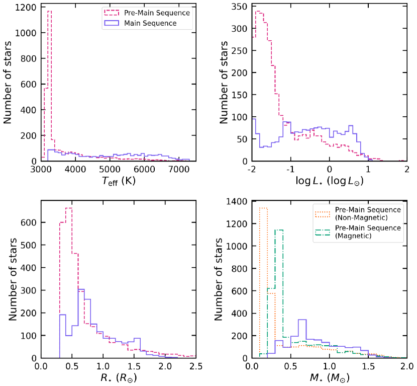
Figure 4: Histograms comparing the stellar properties of our pre-main sequence and main-sequence stars showing effective temperatures (upper left), luminosities (upper right), radii (lower left), and masses (lower right). In all panels, the main sequence distribution is depicted in purple. For the effective temperatures, luminosities, and radii panels, the pre-main sequence distribution is in pink. In the mass panel, we show the pre-main sequence masses from non-magnetic (orange) and magnetic (green) stellar isochrones to highlight the different distributions.

4 The Effect of Stellar properties on Survey Completeness

The intrinsic occurrence rate of planets ($\eta$) can be calculated from the fraction of stars with detected planets in a survey and the survey completeness as follows:

$$\eta=\frac{{n_{\text{p}}}}{n_{\star}}\times\frac{1}{comp_{\text{bin}}}$$ (4)

where $comp_{\text{bin}}$ is the survey completeness evaluated in a discrete radius and orbital period bin, $n_{p}$ is the number of detected planets in the bin and $n_{\star}$ is the number of surveyed stars. The survey completeness is computed by combining the detection efficiency (calculated using injection-recovery tests), and the geometric transit probability, which is given by

$$f_{\text{geo}}=\frac{R_{\star}}{a}$$ (5)

where $R_{\star}$ is the stellar radius, and $a$ is the average semi-major axis, which is calculated from the orbital period using Kepler’s third law. The uncertainty on the occurrence rate was calculated from the square root of the number of detected planets in the bin, assuming Poisson statistics.

In our preliminary analysis of short-period planets in young clusters (Fernandes et al., 2022), we searched five clusters with ten known transiting planets: Tucana-Horologium Association, IC 2602, Upper Centaurus Lupus, Ursa Major, and Pisces-Eridanus. We ran the TESS Primary Mission Full Frame Images (FFIs; 30-min cadence) through our pipeline pterodactyls (Fernandes, 2022) and recovered seven of the eight confirmed planets and one of the two planet candidates. Here, it is important to reiterate that these clusters were solely selected to be used as a test sample to evaluate the effectiveness of our code in recovering these known planets. We specifically focused on sub-Neptunes and Neptunes (0.017–0.055 $\frac{R_{\text{p}}}{R_{\star}}$ or 1.8–6 $R_{\oplus}$, assuming a solar radius for the host star) with orbital periods $<12.5$ days (about half a TESS sector) to better understand the primordial population of sub-Neptunes and Neptunes before they are stripped of their atmospheres. Using Gaia, we took into account the flux contamination prominent in young cluster environments, and computed our detection efficiency in $\frac{R_{\text{p}}}{R_{\star}}$ space because, at the time, most stars in our clusters lacked stellar properties. Given the lack of a homogeneous stellar catalog, we previously included stars of all spectral types in the analysis of our detection efficiency. With an average detection efficiency of 9% and geometric transit probability ($f_{\text{geo}}$) of 0.1 (at a geometric mean orbital period of 3.5 days and assuming a solar-type star), we computed an occurrence rate of 49$\pm$20% for sub-Neptunes and Neptunes in our biased sample of young clusters. This is much higher than the Kepler Gyr-old FGK (Sun-like) occurrence rate of 6.8$\pm$0.3% in the same planet radius and orbital period bin. In this section, we revisited that number using the radii and masses calculated from our homogeneous approach.

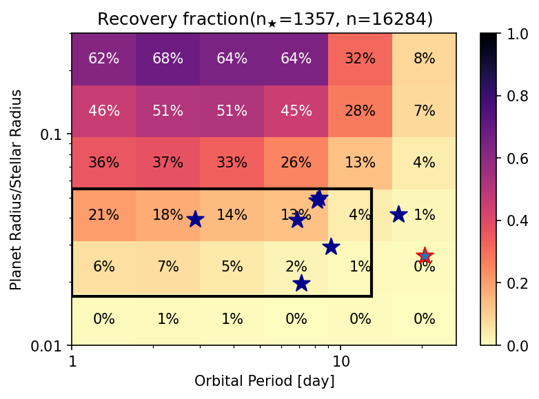
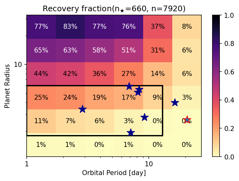
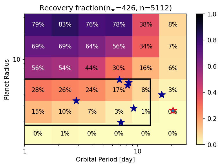
Figure 5: Comparison of detection efficiencies of the sample analyzed in Fernandes et al. (2022). The confirmed planets are depicted using blue stars, except for TOI 1726 b whose recovery required changing pterodactyls. Darker bins represent regions of higher detection efficiency. ${n_{\star}}$ is the total number of stars in our sample while n is the total number of injections done. Black box denotes the bin over which the intrinsic occurrence rates were calculated i.e., sub-Neptunes and Neptunes (0.017–0.055 $\frac{R_{\text{p}}}{R_{\star}}$ or 1.8–6 $R_{\oplus}$, assuming a solar radius) within an orbital period of 12.5 days (about half a TESS sector). Top Left: Detection efficiency of all 1357 stars in $\frac{R_{\text{p}}}{R_{\star}}$-period space before stellar characterization. Top Right: Detection efficiency in planet radius-orbital period space of 660 stars for which we were able to compute stellar properties. Bottom: Detection efficiency in planet radius-orbital period space of 426 FGK (0.55–1.63 $M_{\odot}$) stars.

In this paper, we computed stellar properties for 660 out of 1357 stars studied in Fernandes et al. (2022), with the remaining stars being too faint or lacking necessary 2MASS and Gaia DR3 photometry. After revising our sub-Neptune and Neptune regime detection efficiency with these updated stellar properties, we found a slight increase in the average detection efficiency from 9% to 10% (Figure 5). However, since the total number of stars decreased by 50%, the occurrence rate of sub-Neptunes and Neptunes increased to 90$\pm$37%. For a better comparison with Kepler’s Gyr-old planet population orbiting Sun-like stars, we analyzed only young stars of FGK spectral type (426 stars; 0.55–1.63 $M_{\odot}$). We observed an average detection efficiency of 15% in the young sub-Neptune and Neptune regime, leading to an occurrence rate of 93$\pm$38%. This is comparable to the 90$\pm$37% for all spectral types, which may be partially due to the removal of faint M dwarf stars that make it harder to detect transiting planets with TESS (Kunimoto et al., 2022).

While this occurrence rate is indeed higher than that of Kepler’s Gyr-old population, even when accounting for the fraction of evaporated sub-Neptunes (Bergsten et al., 2022), it is still heavily biased given that we only looked at clusters that are known to have planets. As such, including clusters without known detected planets would lead to a lower occurrence rate. In fact, given that we now know that there are $\sim$2300 Sun-like stars, and 15 published planets in our sample of nearby ($<$200 pc) young clusters and moving groups, assuming the same detection efficiency, the occurrence would drop to 43$\pm$11%, which is effectively the same as the value of 49$\pm$20% that we computed in Fernandes et al. (2022). This observed increase in the occurrence rate of sub-Neptunes and Neptunes could indicate a surplus of these planets at young ages. In future work, as we expand our sample to include data from all nearby clusters and moving groups, it will be important to determine whether this increase in occurrence rate persists when working with a non-biased sample. If it does, it could be due to the fact that the atmospheres of these young sub-Neptunes and Neptunes have not yet been stripped by photoevaporation or core-powered mass loss.

5 Summary and Discussion

The discovery and characterization of transiting exoplanets is strongly dependent on our understanding of their host star properties. In this paper, we used Gaia and 2MASS photometry along with stellar (magnetic and non-magnetic) isochrones in order to derive a homogeneous set of stellar properties, specifically $T_{\text{eff}}$, $L_{\star}$, $R_{\star}$, and $M_{\star}$ for 4,865 stars (1,824 main sequence, and 3,041 pre-main sequence) from 31 nearby ($\sim$200 pc) young ($<$1 Gyr) clusters and moving groups. We found that:

• Our photometrically-derived $T_{\text{eff}}$ values generally agree within measurement uncertainties to those derived from spectroscopic surveys APOGEE and GALAH and LAMOST for both main sequence populations. There are some discrepancies, however, for pre-main sequence stars, which we attribute to spectroscopic surveys using stellar models tuned to main sequence stars.

• Our $T_{\text{eff}}$ values typically agree within measurement uncertainties to those derived in Román-Zúñiga et al. (2023) using APOGEE spectra. Our non-M dwarf luminosities and radii increasingly deviate toward earlier-type stars, which we attribute to differences in accounting for interstellar extinction.

• For FGK type stars, we found that there was no difference in the masses derived from non-magnetic vs. magnetic stellar isochrones. On the other hand, for pre-main sequence M dwarfs (0.1–0.5 $M_{\odot}$), our masses derived from magnetic stellar isochrones are visually more consistent with those derived in Román-Zúñiga et al. (2023), however, our measurement uncertainties are on the order of 100% for this population, making it difficult to conclusively rule out non-magnetic measurements. Though, Simon et al. (2019) found that non-magnetic stellar isochrones tend to underestimate stellar masses, which is consistent with what we see here.

• Given that the median age of our sample is $\sim$45–50 Myr, most of the M dwarfs in our sample have not yet reached the main sequence. We also note a marked decrease in the number of earlier-type pre-main sequence stars with respect to main sequence stars.

• When we took stellar properties into account, there is an overall increase in our detection efficiency. This effect is particularly noticeable among sub-Neptunes/Neptunes (1.8–6 $R_{\oplus}$) where we found a $1.5\times$ increase in the detection efficiency, implying that better characterization of host star properties can lead to the recovery of more smaller transiting planets.

The occurrence rates of sub-Neptunes/Neptunes (1.8–6 $R_{\oplus}$) with orbital periods less than 12.5 days for the 660 stars (out of 1357) for which we could compute stellar properties is 90$\pm$37%. This is significantly higher than Kepler’s Gyr-old occurrence rates of 6.8$\pm$0.3% even when accounting for evaporated sub-Neptunes (Bergsten et al., 2022), as well as our previously calculated 49$\pm$20% (Fernandes et al., 2022) when considering stars of all spectral types in $\frac{R_{\text{p}}}{R_{\star}}$ space. When considering only young stars of FGK spectral type (426 stars; 0.55–1.63 $M_{\odot}$), we computed an occurrence of 93$\pm$38%, which is effectively the same as 90$\pm$37% when considering all stars with stellar properties. While the number of detected planets has not changed, the difference can be attributed to two factors: (1) the total number of only FGK stars is $\sim$1.5 times lower, and (2) the detection efficiency is $\sim$1.5 times higher. While the planet occurrence rate we calculated for our sample is higher than that for Kepler’s Gyr old stars, we realize that this value is biased since we only considered clusters with confirmed/candidate planets. We can further improve upon this by including all of the $>$30 young short-period transiting planets as well as an unbiased sample of nearby clusters and moving groups using light curves from the TESS Extended Mission FFIs. Our homogeneously derived catalog of updated stellar properties will be a crucial input to the accurate estimation of the occurrence rates of young planets. With this young population of transiting, short-period planets, we hope to improve upon the intrinsic occurrence rates calculations, establish how the radius distribution of transiting exoplanets evolved over time, and therefore provide observational constraints on the mass loss mechanisms of planetary atmospheres.

Appendix A Summary of Young Clusters and Moving Groups

Cluster/Moving Group	Distance (in pc)	Age (in Myr)	Total	# in Gaia	# in 2MASS	# in PMS	# in MS
118 Tau	100$\pm$10	$\sim$10	15	15	15	4	3
32 Ori	96$\pm$2	$22^{+4}_{-3}$	42	41	41	5	8
AB Doradus MG	$30^{+20}_{-10}$	$149^{+51}_{-19}$	596	594	539	79	113
Alpha Persei	$\sim$200	90	740	740	717	368	75
Argus	$\sim$120	40-50	38	38	37	5	14
Beta Pictoris	$30^{+20}_{-10}$	24$\pm$3	303	302	271	69	51
Blanco 1	253	132	489	489	481	98	189
Carina	60$\pm$20	$30^{+11}_{-7}$	123	123	114	46	12
CarinaNear	30$\pm$20	$\sim$200	183	183	161	20	27
Coma Bernices	$\sim$85	$562^{+98}_{-84}$	165	165	160	4	64
Columba	50$\pm$20	$42^{+6}_{-4}$	220	220	200	49	44
Eta Cha	95$\pm$1	11$\pm$3	18	18	18	7	0
Hyades	40-50	750$\pm$100	612	612	573	91	146
IC 2391	149$\pm$6	50$\pm$5	333	333	328	151	34
IC 2602	149$\pm$5	$46^{+6}_{-5}$	504	504	477	253	29
Lower Centaurus Crux	110$\pm$10	15$\pm$3	530	529	500	144	62
Mu Tau	150	60	566	566	509	143	70
NGC 2451	180-360	50-80	400	400	380	197	35
Octans	$130^{+30}_{-20}$	35$\pm$5	159	159	151	32	40
Pisces-Eridanus	80-226	120	254	254	250	48	114
Platais 8	130$\pm$10	60	35	35	33	4	12
Pleiades	134$\pm$9	112$\pm$5	1593	1590	1545	467	253
Praesepe	179$\pm$3	790$\pm$60	860	860	835	226	265
Tucana Horologium Association	$46^{+8}_{-6}$	45$\pm$4	212	211	205	85	15
TW Hydra	60$\pm$10	10$\pm$3	86	86	73	17	2
Upper Centaurus Lupus	130$\pm$20	16$\pm$2	936	934	903	248	101
Upper CrA	147$\pm$7	$\sim$10	41	41	38	21	1
Ursa Major	$\sim$25	414$\pm$23	17	17	16	0	5
Upper Scorpius	130$\pm$20	10$\pm$3	411	411	395	149	10
Volans Carina	75-100	$89^{+5}_{-7}$	86	86	82	8	25
XFOR	$\sim$100	$\sim$40	17	17	17	3	5
Total			10,585	10,573	10,064	3,041	1,824

Table 3: Moving groups and clusters whose properties were derived in this work. Distance, age, and membership are from the Gagné et al. (2018) and Babusiaux et al. (2018).

References

- Abdurro’uf et al. (2022) Abdurro’uf, Accetta, K., Aerts, C., et al. 2022, ApJS, 259, 35
- Andrae et al. (2018) Andrae, R., Fouesneau, M., Creevey, O., et al. 2018, A&A, 616, A8
- Babusiaux et al. (2018) Babusiaux, C., van Leeuwen, F., Barstow, M., et al. 2018, Astronomy & astrophysics, 616, A10
- Bailer-Jones et al. (2021) Bailer-Jones, C. A. L., Rybizki, J., Fouesneau, M., Demleitner, M., & Andrae, R. 2021, AJ, 161, 147
- Berger et al. (2020) Berger, T. A., Huber, D., van Saders, J. L., et al. 2020, arXiv e-prints, arXiv:2001.07737
- Bergsten et al. (2022) Bergsten, G. J., Pascucci, I., Mulders, G. D., Fernandes, R. B., & Koskinen, T. T. 2022, arXiv e-prints, arXiv:2209.04047
- Borucki et al. (2010) Borucki, W. J., Koch, D., Basri, G., et al. 2010, Science, 327, 977
- Bouma et al. (2020) Bouma, L., Hartman, J., Brahm, R., et al. 2020, The Astronomical Journal, 160, 239
- Bressan et al. (2012) Bressan, A., Marigo, P., Girardi, L., et al. 2012, MNRAS, 427, 127
- Brown et al. (2011) Brown, T. M., Latham, D. W., Everett, M. E., & Esquerdo, G. A. 2011, AJ, 142, 112
- Buder et al. (2021) Buder, S., Sharma, S., Kos, J., et al. 2021, MNRAS, 506, 150
- Busso et al. (2021) Busso, G., Cacciari, C., Bellazzini, M., et al. 2021, Gaia EDR3 documentation Chapter 5: Photometric data, Gaia EDR3 documentation, European Space Agency; Gaia Data Processing and Analysis Consortium.
- Cardelli et al. (1989) Cardelli, J. A., Clayton, G. C., & Mathis, J. S. 1989, ApJ, 345, 245
- Cody et al. (2014) Cody, A. M., Stauffer, J., Baglin, A., et al. 2014, AJ, 147, 82
- Cui et al. (2012) Cui, X.-Q., Zhao, Y.-H., Chu, Y.-Q., et al. 2012, Research in Astronomy and Astrophysics, 12, 1197
- Curtis et al. (2019) Curtis, J. L., Agüeros, M. A., Mamajek, E. E., Wright, J. T., & Cummings, J. D. 2019, AJ, 158, 77
- Dietrich et al. (2023) Dietrich, J., Apai, D., Schlecker, M., et al. 2023, AJ, 165, 149
- Dressing et al. (2019) Dressing, C. D., Hardegree-Ullman, K., Schlieder, J. E., et al. 2019, AJ, 158, 87
- Duchêne & Kraus (2013) Duchêne, G., & Kraus, A. 2013, Annual Review of Astronomy and Astrophysics, 51, 269
- El-Badry et al. (2021) El-Badry, K., Rix, H.-W., & Heintz, T. M. 2021, MNRAS, 506, 2269
- Ercolano & Pascucci (2017) Ercolano, B., & Pascucci, I. 2017, Royal Society Open Science, 4, 170114
- Fang et al. (2021) Fang, M., Kim, J. S., Pascucci, I., & Apai, D. 2021, ApJ, 908, 49
- Fang et al. (2023) Fang, M., Pascucci, I., Edwards, S., et al. 2023, ApJ, 945, 112
- Feiden (2016) Feiden, G. A. 2016, A&A, 593, A99
- Feinstein et al. (2019) Feinstein, A. D., Montet, B. T., Foreman-Mackey, D., et al. 2019, Publications of the Astronomical Society of the Pacific, 131, 094502
- Fernandes (2022) Fernandes, R. 2022, pterodactyls: A Tool to Uniformly Search and Vet for Young Transiting Planets In TESS Primary Mission Photometry, doi:10.5281/zenodo.6667960
- Fernandes et al. (2022) Fernandes, R. B., Mulders, G. D., Pascucci, I., et al. 2022, AJ, 164, 78
- Fulton et al. (2017) Fulton, B. J., Petigura, E. A., Howard, A. W., et al. 2017, The Astronomical Journal, 154, 109
- Gagné et al. (2020) Gagné, J., David, T. J., Mamajek, E. E., et al. 2020, ApJ, 903, 96
- Gagné et al. (2018) Gagné, J., Mamajek, E. E., Malo, L., et al. 2018, The Astrophysical Journal, 856, 23
- Gaia Collaboration et al. (2016) Gaia Collaboration, Prusti, T., de Bruijne, J. H. J., et al. 2016, A&A, 595, A1
- Gaia Collaboration et al. (2018) Gaia Collaboration, Brown, A. G. A., Vallenari, A., et al. 2018, A&A, 616, A1
- Gaia Collaboration et al. (2021) —. 2021, A&A, 649, A1
- Gaia Collaboration et al. (2022a) Gaia Collaboration, Arenou, F., Babusiaux, C., et al. 2022a, arXiv e-prints, arXiv:2206.05595
- Gaia Collaboration et al. (2022b) Gaia Collaboration, Vallenari, A., Brown, A. G. A., et al. 2022b, arXiv e-prints, arXiv:2208.00211
- Giacalone et al. (2021) Giacalone, S., Dressing, C. D., Jensen, E. L. N., et al. 2021, AJ, 161, 24
- Ginzburg et al. (2016) Ginzburg, S., Schlichting, H. E., & Sari, R. 2016, The Astrophysical Journal, 825, 29
- Ginzburg et al. (2018) —. 2018, Monthly Notices of the Royal Astronomical Society, 476, 759
- Green (2018) Green, G. M. 2018, The Journal of Open Source Software, 3, 695
- Green et al. (2019) Green, G. M., Schlafly, E., Zucker, C., Speagle, J. S., & Finkbeiner, D. 2019, ApJ, 887, 93
- Gupta & Schlichting (2019) Gupta, A., & Schlichting, H. E. 2019, Monthly Notices of the Royal Astronomical Society, 487, 24
- Gupta & Schlichting (2020) Gupta, A., & Schlichting, H. E. 2020, MNRAS, 493, 792
- Gupta & Schlichting (2020) Gupta, A., & Schlichting, H. E. 2020, Monthly Notices of the Royal Astronomical Society, 493, 792
- Hardegree-Ullman et al. (2020) Hardegree-Ullman, K. K., Zink, J. K., Christiansen, J. L., et al. 2020, The Astrophysical Journal Supplement Series, 247, 28
- Hedges (2021) Hedges, C. 2021, Research Notes of the AAS, 5, 262
- Hertzsprung (1911) Hertzsprung, E. 1911, Publikationen des Astrophysikalischen Observatoriums zu Potsdam, 63
- Hippke et al. (2019) Hippke, M., David, T. J., Mulders, G. D., & Heller, R. 2019, The Astronomical Journal, 158, 143
- Hippke & Heller (2019) Hippke, M., & Heller, R. 2019, Astronomy & Astrophysics, 623, A39
- Howell et al. (2014) Howell, S. B., Sobeck, C., Haas, M., et al. 2014, Publications of the Astronomical Society of the Pacific, 126, 398
- Huber et al. (2016) Huber, D., Bryson, S. T., Haas, M. R., et al. 2016, ApJS, 224, 2
- Hunter (2007) Hunter, J. D. 2007, Computing in Science & Engineering, 9, 90
- Jones et al. (2001–) Jones, E., Oliphant, T., Peterson, P., et al. 2001–, SciPy: Open source scientific tools for Python, [Online; accessed ¡today¿]
- Kunimoto et al. (2022) Kunimoto, M., Daylan, T., Guerrero, N., et al. 2022, ApJS, 259, 33
- Luhman (2020) Luhman, K. L. 2020, AJ, 160, 186
- Mamajek et al. (2015) Mamajek, E. E., Torres, G., Prsa, A., et al. 2015, arXiv e-prints, arXiv:1510.06262
- Mann et al. (2015) Mann, A. W., Feiden, G. A., Gaidos, E., Boyajian, T., & von Braun, K. 2015, ApJ, 804, 64
- Mann et al. (2019) Mann, A. W., Dupuy, T., Kraus, A. L., et al. 2019, ApJ, 871, 63
- Mann et al. (2020) Mann, A. W., Johnson, M. C., Vanderburg, A., et al. 2020, The Astronomical Journal, 160, 179
- Mulders et al. (2018) Mulders, G. D., Pascucci, I., Apai, D., & Ciesla, F. J. 2018, AJ, 156, 24
- Nardiello et al. (2020) Nardiello, D., Piotto, G., Deleuil, M., et al. 2020, Monthly Notices of the Royal Astronomical Society, 495, 4924
- Newton et al. (2019) Newton, E. R., Mann, A. W., Tofflemire, B. M., et al. 2019, The Astrophysical Journal Letters, 880, L17
- Newton et al. (2021) Newton, E. R., Mann, A. W., Kraus, A. L., et al. 2021, The Astronomical Journal, 161, 65
- Owen & Wu (2013) Owen, J. E., & Wu, Y. 2013, The Astrophysical Journal, 775, 105
- Owen & Wu (2017) —. 2017, The Astrophysical Journal, 847, 29
- Pascucci et al. (2016) Pascucci, I., Testi, L., Herczeg, G. J., et al. 2016, ApJ, 831, 125
- Pecaut & Mamajek (2013) Pecaut, M. J., & Mamajek, E. E. 2013, ApJS, 208, 9
- Ricker et al. (2014) Ricker, G. R., Winn, J. N., Vanderspek, R., et al. 2014, Journal of Astronomical Telescopes, Instruments, and Systems, 1, 014003
- Rizzuto et al. (2020) Rizzuto, A. C., Newton, E. R., Mann, A. W., et al. 2020, The Astronomical Journal, 160, 33
- Rogers et al. (2021) Rogers, J. G., Gupta, A., Owen, J. E., & Schlichting, H. E. 2021, MNRAS, 508, 5886
- Román-Zúñiga et al. (2023) Román-Zúñiga, C. G., Kounkel, M., Hernández, J., et al. 2023, AJ, 165, 51
- Russell (1914) Russell, H. N. 1914, Popular Astronomy, 22, 275
- Salama et al. (2022) Salama, M., Ziegler, C., Baranec, C., et al. 2022, AJ, 163, 200
- Schlafly & Finkbeiner (2011) Schlafly, E. F., & Finkbeiner, D. P. 2011, ApJ, 737, 103
- Schlegel et al. (1998) Schlegel, D. J., Finkbeiner, D. P., & Davis, M. 1998, ApJ, 500, 525
- Simon et al. (2019) Simon, M., Guilloteau, S., Beck, T. L., et al. 2019, ApJ, 884, 42
- Skrutskie et al. (2006) Skrutskie, M. F., Cutri, R. M., Stiening, R., et al. 2006, AJ, 131, 1163
- Stassun et al. (2018) Stassun, K. G., Oelkers, R. J., Pepper, J., et al. 2018, AJ, 156, 102
- Stassun et al. (2019) Stassun, K. G., Oelkers, R. J., Paegert, M., et al. 2019, AJ, 158, 138
- Torres et al. (2010) Torres, G., Andersen, J., & Giménez, A. 2010, A&A Rev., 18, 67
- van der Walt et al. (2011) van der Walt, S., Colbert, S. C., & Varoquaux, G. 2011, Computing in Science & Engineering, 13, 22
- Van Eylen et al. (2018) Van Eylen, V., Agentoft, C., Lundkvist, M., et al. 2018, Monthly Notices of the Royal Astronomical Society, 479, 4786
- Wang & Chen (2019) Wang, S., & Chen, X. 2019, ApJ, 877, 116
- Zellem et al. (2020) Zellem, R. T., Pearson, K. A., Blaser, E., et al. 2020, Publications of the Astronomical Society of the Pacific, 132, 054401
- Ziegler et al. (2020) Ziegler, C., Tokovinin, A., Briceño, C., et al. 2020, AJ, 159, 19
- Zink (2019) Zink, J. 2019, jonzink/EDI-Vetter: Initial Release, doi:10.5281/zenodo.3585940
- Zuckerman (2019) Zuckerman, B. 2019, ApJ, 870, 27