Abstract

This paper is concerned with signal detection in Gaussian noise under quadratically convex orthosymmetric (QCO) constraints. Specifically the null hypothesis assumes no signal, whereas the alternative considers signal which is separated in Euclidean norm from zero, and belongs to the QCO constraint. Our main result establishes the minimax rate of the separation radius between the null and alternative purely in terms of the geometry of the QCO constraint — we argue that the Kolmogorov widths of the constraint determine the critical radius. This is similar to the estimation problem with QCO constraints, which was first established by Donoho et al., (1990); however, as expected, the critical separation radius is smaller compared to the minimax optimal estimation rate. Thus signals may be detectable even when they cannot be reliably estimated.

1 Introduction

In this short note we study the problem of minimax optimal signal detection in Gaussian noise under quadratically convex orthosymmetric (QCO) constraints. We call a set $K\subset\mathbb{R}^{n}$ (or $\ell_{2}$) quadratically convex if it is convex and in addition the set $K^{2}=\{\theta^{2}:\theta\in K\}$, where $\theta^{2}$ is $\theta$ squared entrywise is convex. A set $K$ is called orthosymmetric if for a vector $\theta\in K$ we have $(\pm\theta_{i})_{i\in I}\in K$ (where $I$ is $[n]=\{1,\ldots,n\}$ or $\mathbb{N}$) for any choice of the signs $\pm$. We are primarily interested in the following problem: let $X=\mu+\xi$ be a single observation, where $\mu\in K$ for a known QCO set $K$, and $\xi_{i}\sim N(0,\sigma^{2})$ for $i\in I$ are independent and identically distributed mean $0$ and known variance equal to $\sigma^{2}$, Gaussian variables. We would like to test whether $H_{0}:\mu=0$ versus the alternative that $H_{A}:\|\mu\|_{2}\geq\rho,\mu\in K$ based on the observation $X$, where $\|\mu\|_{2}$ denotes the $\ell_{2}$ norm of $\mu$. We are interested in characterizing the smallest value of $\rho$ (up to constant factors) for which testing this problem becomes possible. See Figure 1 for an illustrative example of the problem.

Figure 1: Testing $H_{0}:\mu=0$ vs $H_{A}:\|\mu\|_{2}\geq\rho,\mu\in K$ for the axis aligned ellipsoid (which is a special case of a QCO set) $K$ based on the observation $X$. Upon applying a rotation to the data, one can use the test we develop in Section 2.2 to solve optimally problems for rotated (non-axis aligned) ellipsoids or more generally QCO sets (who are still centered at the $0$ point). See our first remark in the discussion section for more details.

Our main result shows that a purely geometrical aspect of the QCO set $K$ drives the optimal critical value of $\rho$. Concretely, suppose we are given a test $\phi_{\alpha}(X)\in\{0,1\}$ such that $\mathbb{P}_{0}(\phi_{\alpha}=1)\leq\alpha$, where $\mathbb{P}_{0}$ denotes the law of $X$ when $\mu=0$. Let

$$\rho(\phi_{\alpha},K,\delta,\sigma):=\inf_{\rho}\{\rho>0:\sup_{\mu:\|\mu\|_{2}\geq\rho,\mu\in K}\mathbb{P}_{\mu}(\phi_{\alpha}=0)\leq\delta\}.$$

We are interested in determining the rate of the expression $\rho(K,\alpha,\delta,\sigma):=\inf_{\phi_{\alpha}}\rho(\phi_{\alpha},K,\delta,\sigma)$ up to universal constants for sufficiently small $\delta$ values, where the inf is taken with respect to all level $\alpha$ tests $\phi_{\alpha}$. We will determine the rate of $\rho(K,\alpha,\delta,\sigma)$ following a standard recipe for such problems: by upper and lower bounding it. The lower bound depends on an information theoretic argument, which is standard in the literature — but in order to apply it we prove a result which shows the existence of certain extremal vectors in a QCO set. The upper bound is achieved through analyzing specific tests: in this paper we propose two minimax optimal tests (which are variants of each other) which both rely on carefully projecting the data in a certain sub-space.

QCO sets were first introduced in Donoho et al., (1990) (see also (Johnstone,, 2019, Chapter 4.8)), where the authors give many examples of such sets, such as hyperrectangles, ellipsoids (both aligned with the coordinate axis), and sets of the form $\{\theta:\sum_{i\in I}a_{i}\psi(\theta_{i}^{2})\leq 1\}$, where $\psi$ is a given convex function and $a_{i}\in\mathbb{R}^{+}$. The last example implies that all unit balls of (weighted) $\ell_{p}$ norms, for $p\geq 2$ are QCO sets. The set of QCO constraints is therefore much larger than simply the sets of all ellipsoids. Unlike the present work which focuses on testing, Donoho et al., (1990) characterized the minimax estimation rates in the corresponding Gaussian sequence model problem. As it turns out the Kolmogorov widths of the set $K$ (see (2.1) for a definition) determine the minimax rate of estimation. We will see that the Kolmogorov widths also determine the minimax rate of testing with QCO constraints, but the rate is strictly smaller. In fact, one of our motivations to study this problem is to exhibit a fundamental difference between the testing and estimation rates. This difference is of course nothing new. In their seminal body of work on nonparametric testing Ingster, (1982); Ingster, 1993a ; Ingster, 1993b ; Ingster, 1993c ; Ingster and Suslina, (2000) showed the difference between testing and estimation in multiple problems. See also Ingster and Suslina, (2003) for a summary of the many existing results in the area. Despite much progress in goodness of fit testing in Gaussian models, we are not aware of a general result dedicated to QCO sets. For certain special types of ellipsoids, the problem was first studied by Ermakov, (1991), where the author derived exact minimax rates. Suslina, (1996) studied the asymptotics of the problem of signal detection in $\ell_{q}$ ellipsoids with $\ell_{p}$ ball removed. Since $\ell_{q}$ ellispoids for $q\geq 2$ are QCO sets, when $p=2$ we provide a generalization of these results. For general ellipsoids, Baraud, (2002) studied the testing problem in $\mathbb{R}^{n}$ and $\ell_{2}$ and obtained the minimax optimal critical radius. Our work can hence be seen as a generalization to part of Baraud, (2002). In an interesting recent work, Wei and Wainwright, (2020) studied local testing rates on ellipsoids. Here local means that the point of interest under the null is not necessarily the zero point, but can be an arbitrary point in the ellipsoid. Wei and Wainwright, (2020) proved upper and lower bounds based on localized Kolmogorov widths, which are not guaranteed to match in general, but do match for certain examples with Sobolev ellipsoids. In contrast, the present work focuses on more general sets, but the point of interest under the null hypothesis is always anchored at the zero point, and the critical radius is determined based on the global (instead of local) Kolmogorov widths of the set.

1.1 Notation

For a vector $v$, which is a collection of entries $(v_{i})_{i\in I}$ (where $I$ is either $[n]$ or $\mathbb{N}$) we use $\|v\|_{1}=\sum_{i\in I}|v_{i}|$, $\|v\|_{2}=\sqrt{\sum_{i\in I}v_{i}^{2}}$ and $\|v\|_{\infty}=\sup_{i\in I}|v_{i}|$. For two vectors $v_{1},v_{2}$ we denote their dot product with $\langle v_{1},v_{2}\rangle=\sum_{i\in I}v_{1,i}v_{2,i}$.

1.2 Organization

The paper is structured as follows. Section 2 proves lower and upper bounds for the signal detection problem and contains the main result of the paper. Section 4 contains a brief discussion comapring the minimax estimation to testing rates, and including some open problems.

2 Main Result

In this section we assume we have a QCO set $K$, and we are testing the problem described in the introduction. Let

$$d_{k}(K)=\inf_{P\in\mathcal{P}_{k}}\sup_{\theta\in K}\|\theta-P\theta\|_{2},$$ (2.1)

be the Kolmogorov widths of the set $K$, where $\mathcal{P}_{k}$ denotes the collection of all projections on subspaces of dimension $k$ (see Pinkus,, 2012, for more details and properites of the Kolmogorov width). Here $d_{k}(K)$ forms a decreasing sequence where $d_{n}(K)=0$ (when $K\subset\mathbb{R}^{n}$) and $\lim_{n\rightarrow\infty}d_{n}(K)$ is assumed to be $0$ for the case when $K\subset\ell_{2}$.

2.1 Lower Bound

The lower bound rests on the following key lemma on the existence of certain extremal vectors in the set $K$.

Lemma 2.1.

Let $K$ be a QCO set. Suppose that $d_{k-1}(K)>\sqrt[4]{k}\sigma$. Then there exists a vector $\theta\in K$ such that $\|\theta\|_{2}^{2}=\sqrt{k}\sigma^{2}$, $\|\theta\|_{\infty}\leq\sigma/\sqrt[4]{k}$.

Proof.

Our proof uses a similar argument to that in Section 3.3.2. in Neykov, (2022), but for completeness we spell out the details. We have the following inequality:

$$\inf_{P\in\mathcal{P}_{k-1}}\sup_{\theta\in K}\|\theta-P\theta\|_{2}^{2}>\sqrt{k}\sigma^{2}.$$

We can only consider projections aligned with the coordinates – there are $n_{k}:={n\choose k-1}$ such projections in the real case, otherwise there are countably many such projections. Denote the index set of such projections with $J$ (i.e. $J=[n_{k}]$ in the real case). We have

$$\inf_{P\in\mathcal{P}_{k-1}}\sup_{\theta\in K}\|\theta-P\theta\|_{2}^{2}\leq\inf_{S}\sup_{\theta\in K}\sum_{i\in I}\theta^{2}_{i}-\sum_{i\in S}\theta_{i}^{2},$$

where the minimum over $S$ is taken with respect to all subsets of $I$ with exactly $k-1$ elements. Since the set is quadratically convex the above can be written as

$$\inf_{P\in\mathcal{P}_{k-1}}\sup_{\theta\in K}\|\theta-P\theta\|_{2}^{2}\leq\inf_{S}\sup_{t\in K^{2}}\sum_{i\in I}t_{i}-\sum_{i\in S}t_{i}=\inf_{w\in S_{k}}\sup_{t\in K^{2}}\|t\|_{1}-\langle w,t\rangle,$$

where $w$ ranges in the set $S_{k}:=\{e:e\in\mathbb{R}^{n}$ or $\ell_{2}$ s.t. $e$ has exactly $k-1$-entries equal to $1$ and the rest are $0\}$. It follows that for each $\varepsilon>0$ and each $w_{i}\in S_{k}$ there exists a $t_{i}$ such that $\|t_{i}\|_{1}-\langle w_{i},t_{i}\rangle\geq\sqrt{k}\sigma^{2}-\varepsilon$. Since the set $K$ is convex and orthosymmetric we may assume without loss of generality that $t_{i}$ has $0$ entries on the support of $w_{i}$ and $\|t_{i}\|_{1}=\|t_{i}\|_{1}-\langle w_{i},t_{i}\rangle=\sqrt{k}\sigma^{2}-\varepsilon$ (the latter holds since the set contains $0$). We will now argue that there exists a convex combination $t_{\alpha}:=\sum_{i\in J}\alpha_{i}t_{i}$ such that $\|t_{\alpha}\|_{\infty}\leq\sigma^{2}/\sqrt{k}$. To see this, first observe that since all $t_{i}$ have positive entries $\|t_{\alpha}\|_{\infty}=\sup_{e:e\geq 0,\|e\|_{1}=1}\langle e,t_{\alpha}\rangle$. Hence it suffices to show that

$$\inf_{\alpha:\alpha\geq 0,\|\alpha\|_{1}=1}\sup_{e:e\geq 0,\|e\|_{1}=1}\langle e,t_{\alpha}\rangle\leq\sigma^{2}/\sqrt{k}.$$

Since both sets over which the optimization is performed are convex, and the function $\langle e,t_{\alpha}\rangle=\sum_{i\in J}\alpha_{i}\langle e,t_{i}\rangle$ is convex-concave (indeed it is linear in both arguments) by the minimax theorem we have

$$\inf_{\alpha:\alpha\geq 0,\|\alpha\|_{1}=1}\sup_{e:e\geq 0,\|e\|_{1}=1}\langle e,t_{\alpha}\rangle=\sup_{e:e\geq 0,\|e\|_{1}=1}\inf_{\alpha:\alpha\geq 0,\|\alpha\|_{1}=1}\langle e,t_{\alpha}\rangle=\sup_{e:e\geq 0,\|e\|_{1}=1}\min_{i\in J}\langle e,t_{i}\rangle.$$

Observe that $\min_{i\in J}\langle e,t_{i}\rangle\leq\langle e,t_{e}\rangle$, where $t_{e}$ is selected such that it has $0$ entries corresponding to the top $k-1$ entries of $e$. Let $U$ denote the set of the top $k-1$ entries of $e$. Thus $\langle e,t_{e}\rangle=\sum_{i\not\in U}e_{i}t_{e,i}\leq\|e_{\setminus U}\|_{\infty}\|t_{e}\|_{1}=\|e_{\setminus U}\|_{\infty}(\sqrt{k}\sigma^{2}-\varepsilon)$, where $e_{\setminus U}$ denotes the vector $e$ with its top $k-1$ entries removed. Finally observe that $\|e_{\setminus U}\|_{\infty}\leq\frac{1}{k}$ since $1=\|e\|_{1}\geq k\|e_{\setminus U}\|_{\infty}$. Hence we conclude that there exists $t^{*}=t_{\alpha^{*}}$ such that

$$\|t^{*}\|_{\infty}\leq\sigma^{2}/\sqrt{k}.$$

In addition since $t^{*}$ is a convex combination of vectors $t_{i}$ we must have $\|t^{*}\|_{1}=\sqrt{k}\sigma^{2}-\varepsilon$, and $t^{*}\in K^{2}$. Taking $\varepsilon\rightarrow 0$ completes the proof. ∎

We now state the main lower bound result. Its proof relies on Le Cam’s method of “fuzzy hypothesis”.

Theorem 2.2.

If $\rho\lesssim\max_{j:d_{j-1}(K)>\sqrt[4]{j}\sigma}\sqrt[4]{j}\sigma$ for some sufficiently small absolute constant then

$$\inf_{\psi:\mathbb{P}_{0}(\psi=1)\leq\alpha}\sup_{\theta\in K,\|\theta\|\geq\rho}\mathbb{P}_{\theta}(\psi=0)\geq\delta,$$

for some sufficiently small $\delta>0$.

Proof.

We start by a classical treatment of minimax testing lower bounds which we take from Baraud, (2002). Let $\mathbb{P}_{\nu}$ denote an arbitrary prior on the set $\mu\in K,\|\mu\|\geq\rho$. We have that

$$\inf_{\psi:\mathbb{P}_{0}(\psi=1)\leq\alpha}\sup_{\mu\in K,\|\mu\|\geq\rho}\mathbb{P}(\psi=0) \geq\inf_{\psi:\mathbb{P}_{0}(\psi=1)\leq\alpha}\mathbb{P}_{\nu}(\psi=0)\geq 1-\alpha-\frac{1}{2}\|\mathbb{P}_{0}-\mathbb{P}_{\nu}\|_{1}.$$

Now let $L_{\nu}=\frac{d\mathbb{P}_{\nu}}{d\mathbb{P}_{0}}$, assuming that $\mathbb{P}_{\nu}\ll\mathbb{P}_{0}$. Then by Cauchy-Schwartz we have

$$\|\mathbb{P}_{0}-\mathbb{P}_{\nu}\|_{1}=\mathbb{E}_{0}|L_{\nu}-1|\leq(\mathbb{E}_{0}[L_{\nu}^{2}]-1)^{1/2}.$$

Hence we conclude

$$\inf_{\psi:\mathbb{P}_{0}(\psi=1)\leq\alpha}\sup_{\mu\in K,\|\mu\|\geq\rho}\mathbb{P}(\psi=0)\geq 1-\alpha-\frac{1}{2}(\mathbb{E}_{0}[L_{\nu}^{2}]-1)^{1/2}.$$

Let $\theta$ be the vector from Lemma 2.1. We will use the prior $(\kappa\gamma_{i}\theta_{i})_{i\in I}\in K$ where $\gamma_{i}$ for $i\in I$ are i.i.d. Rademacher random variables for some small constant $0<\kappa<1$. Observe that all these variables have squared Euclidean norm (at least) equal to $\rho^{2}=\sqrt{k}\kappa^{2}\sigma^{2}$. Denote the corresponding mixture measure by $\mathbb{P}_{\nu}$.

Calculating the $\chi^{2}$-divergence of this mixture we obtain:

$$\mathbb{E}_{0}(L_{\nu})^{2}-1 =\mathbb{E}_{\nu,\nu^{\prime}}\mathbb{E}_{Y\sim N(0,\sigma^{2}\mathbb{I}_{n})}\frac{\exp(-\|Y-\nu\|_{2}^{2}/2\sigma^{2})\exp(-\|Y-\nu^{\prime}\|_{2}^{2}/2\sigma^{2})}{\exp(-\|Y\|_{2}^{2}/\sigma^{2})}-1$$

$$=\mathbb{E}_{\nu,\nu^{\prime}}\exp(\nu{{}^{\mathrm{\scriptscriptstyle T}}}\nu^{\prime}/\sigma^{2})-1,$$

where by $\mathbb{E}_{\nu,\nu^{\prime}}$ we mean expectation over two i.i.d. draws from the prior distribution that we specified above. By symmetry in the above we can fix $\nu=\kappa\theta$. Next we have

$$\mathbb{E}_{\nu,\nu^{\prime}}\exp(\nu{{}^{\mathrm{\scriptscriptstyle T}}}\nu^{\prime}/\sigma^{2})-1 =\prod_{i\in I}\cosh(\kappa^{2}\theta_{i}^{2}/\sigma^{2})-1\leq\exp(\sum_{i\in I}\theta_{i}^{4}\kappa^{4}/(2\sigma^{4}))-1$$

$$\leq\exp(\|\theta\|^{2}_{\infty}\|\theta\|^{2}_{2}\kappa^{4}/(2\sigma^{4}))-1\leq\exp(\kappa^{4}/2)-1,$$

where we used the well known inequality $\cosh(x)\leq\exp(x^{2}/2)$ which can be checked by comparing the Taylor series, and the properties of $\theta$ from Lemma 2.1. It follows that for sufficiently large $\kappa$ the minimax risk for testing is lower bounded by

$$1-\alpha-\frac{1}{2}(\exp(\kappa^{4}/2)-1)^{1/2}.$$

Thus we conclude that if $\rho\lesssim\max_{j:d_{j-1}(K)\geq\sqrt[4]{j}\sigma}\sqrt[4]{j}\sigma$ minimax testing is not possible. ∎

2.2 Upper Bound

Note that for the upper bound by adding and subtracting $\eta\sim N(0,\sigma^{2}\mathbb{I}_{n})$ to $X$, we can double the sample at the expense of increasing the variance. So for this section we will assume that we have two independent samples $X,Y\sim N(0,2\sigma^{2}\mathbb{I}_{n})$ or $X,Y\sim N(\mu,2\sigma^{2}\mathbb{I}_{n})$. Let $P^{*}_{k}$ (nearly) achieve the inf for $d_{k}(K)$ (if the inf is not achieved then we can take a sequence of projections which achieves it in the limit so that the following logic continues to work). For the upper bound under the alternative, we can notice that for any $\mu\in K,\|\mu\|_{2}\geq\rho$ we have by the Pythagorean theorem $\|P^{*}_{k}\mu\|_{2}^{2}=\|\mu\|_{2}^{2}-\|P^{*}_{k}\mu-\mu\|_{2}^{2}\geq\rho^{2}-d^{2}_{k}(K)$. We consider $Z=|Z^{\prime}|$, where

$$Z^{\prime}=X{{}^{\mathrm{\scriptscriptstyle T}}}P_{k}^{*}Y,$$ (2.2)

as a test statistic, and our test $\psi=\mathbbm{1}(|X{{}^{\mathrm{\scriptscriptstyle T}}}P_{k}^{*}Y|>2\sqrt{\alpha^{-1}}\sigma^{2}\sqrt{k})$ (we propose an alternative test in the simulation section which also achieves minimax optimal power; this alternative test is very related to the test proposed here but has a slightly more involved analysis). Under the null hypothesis the statistic $Z^{\prime}$, clearly has expectation $0$ and the variance equals to

$$\mathbb{E}((P_{k}^{*}X){{}^{\mathrm{\scriptscriptstyle T}}}P_{k}^{*}Y)^{2}=\mathbb{E}\langle XX{{}^{\mathrm{\scriptscriptstyle T}}}P_{k}^{*},P_{k}^{*}YY{{}^{\mathrm{\scriptscriptstyle T}}}\rangle=\langle 2\sigma^{2}P_{k}^{*},2\sigma^{2}P_{k}^{*}\rangle=4\sigma^{4}k,$$ (2.3)

where we used the standard dot product between matrices $\langle A,B\rangle=\operatorname{tr}(A{{}^{\mathrm{\scriptscriptstyle T}}}B)$ and the independence between $X$ and $Y$. It follows by Chebyshev’s inequality that

$$\mathbb{P}(Z\geq 2C\sigma^{2}\sqrt{k})\leq 1/C^{2}.$$

Hence we can select $C=\sqrt{\alpha^{-1}}$ to control the type I error below $\alpha$.

Under the alternative we use the approach of Diakonikolas et al., (2022). The expected value of the statistic $Z^{\prime}$ under the alternative is $\|P_{k}^{*}\mu\|_{2}^{2}\geq\rho^{2}-d^{2}_{k}(K)$. Observe that $\sqrt{\mathbb{E}Z^{2}}=\sqrt{\mathbb{E}Z^{\prime 2}}\geq\mathbb{E}Z^{\prime}\geq\rho^{2}-d^{2}_{k}(K)$. By Carberry-Wright’s inequality (see Fact 2.1 of Diakonikolas et al., (2022) and also Carbery and Wright, (2001)) we then have:

$$\mathbb{P}(Z<2C\sigma^{2}\sqrt{k}) =\mathbb{P}(Z<2C\sigma^{2}\sqrt{k}\sqrt{\mathbb{E}Z^{2}}/\sqrt{\mathbb{E}Z^{2}})\leq C_{*}\sqrt{\frac{2C\sigma^{2}\sqrt{k}}{\sqrt{\mathbb{E}Z^{2}}}}$$

$$\leq C_{*}\sqrt{\frac{2C\sigma^{2}\sqrt{k}}{\rho^{2}-d^{2}_{k}(K)}}<\delta,$$

when $\rho^{2}\geq d^{2}_{k}(K)+C_{*}^{2}\delta^{-2}(\sigma^{2}2C\sqrt{k})$. Since we are allowed to take any $k$ for this test we conclude that the upper bound is possible whenever $\rho^{2}\gtrsim\min_{j\in\{1,\ldots,n\}}d^{2}_{j}(K)+\sigma^{2}\sqrt{j}$ or $\rho^{2}\gtrsim\min_{j\in\mathbb{N}}d^{2}_{j}(K)+\sigma^{2}\sqrt{j}$ for the case when $K$ is a subset of $\ell_{2}$.

2.3 Main Result

Theorem 2.3.

Suppose that $j^{*}\in I$ is such that $d_{j^{*}-1}(K)>\sqrt[4]{j^{*}}\sigma$ but $d_{j^{*}}(K)\leq\sqrt[4]{j^{*}+1}\sigma$. Then the minimax optimal rate of the critical radius satisfies $\rho(K,\alpha,\delta,\sigma)\asymp\sqrt[4]{j^{*}}\sigma$ for sufficiently small $\delta>0$. On the other hand suppose that $d_{0}(K)\leq\sigma$, then $\rho(K,\alpha,\delta,\sigma)\geq d_{0}(K)$ for small enough $\delta>0$, so that testing is impossible in this case.

Proof.

From the lower bound we immediately conclude that the rate is at least $\sqrt[4]{j^{*}}\sigma$. On the other hand the upper bound grants the rate $\sigma\sqrt{(\sqrt{j^{*}+1}+\sqrt{j^{*}})}\asymp\sqrt[4]{j^{*}}\sigma$. The only corner case we need to consider is when $d_{0}(K)\leq\sigma$. In that case we can find a point $\theta\in K$ such that $\|\theta\|=d_{0}(K)\leq\sigma$. Considering $\gamma\theta$ for a Rademacher variable $\gamma$, gives that the $\chi^{2}$ divergence will be bounded by $\cosh(\|\theta\|_{2}^{2}/\sigma^{2})-1\leq\exp(\|\theta\|^{4}_{2}/(2\sigma^{4}))-1$ which is small, and therefore the minimax rate of testing is at least $d_{0}(K)$ for small enough $\delta$ which means it is impossible to test this problem. ∎

3 Simulation Studies

We begin this section by defining an alternative minimax optimal test, to the one defined in Section 2.2. The analysis of this test is slightly more involved, however for a fixed value of $\|\mu\|_{2}$ we can derive the minimal power of this test, which makes for a nice power-plot. We now define the test (which is really just a variant of the one proposed in Section 2.2) and state several lemmas which together characterize its minimal power. After that we attach the simulation studies.

Consider the test statistic $T^{\prime}=\max(Z^{\prime},0)$ where $Z^{\prime}$ is defined in (2.2). We will now argue that the test $\psi=\mathbbm{1}(T^{\prime}\geq 2\sqrt{\alpha^{-1}}\sigma^{2}\sqrt{k})$ also works at a minimax optimal rate (although the proof, which relies on Paley-Zygmund’s inequality, is slightly more cumbersome than the one presented in Section 2.2, so we prefer to exhibit both tests).

Lemma 3.1.

Given $k\in I$, the test $\psi$ as defined above, with $P_{k}^{*}$, satisfies that the type I error is below $\alpha$, and the type II error is $\leq 1-f(C)$ for some $f(C)\rightarrow 0$ as $C\rightarrow\infty$ as long as $\rho^{2}=\|\mu\|^{2}_{2}\geq d^{2}_{k}(K)+C\sqrt{k}\sigma^{2}$.

The proof of Lemma 3.1 and all subsequent lemmas of this section are deferred to the appendix. Lemma 3.1 simply argues that $\psi$ is minimax optimal, whenever $k$ is the optimal index defined as in Theorem 2.3, i.e., $k$ satisfies

$$d_{k-1}(K)>\sqrt[4]{k}\sigma,\mbox{ but }d_{k}(K)\leq\sqrt[4]{k+1}\sigma.$$ (3.1)

We now state our result characterizing when $\psi$ has minimal power.

Lemma 3.2.

For two vectors $\mu,\mu^{\prime}\in K$ and data points $X=\mu+\xi$, $Y=\mu+\eta$ and $X^{\prime}=\mu^{\prime}+\xi$ and $Y^{\prime}=\mu^{\prime}+\eta$, where $\xi,\eta\sim N(0,2\sigma^{2}\mathbb{I})$ the statistic $XP_{k}^{*}Y$ (first-order) stochastically dominates $X^{\prime}P_{k}^{*}Y^{\prime}$ when $\|P_{k}^{*}\mu\|_{2}\geq\|P_{k}^{*}\mu^{\prime}\|_{2}$. This implies that the test $\psi$ defined in this section, has increasing power in the parameter $\|P_{k}^{*}\mu\|_{2}$.

It follows that for a given norm $\|\mu\|_{2}=c$ if we want to derive the minimal power of $\psi$ we simply need to find a point $\mu\in K$ such that $\|\mu\|_{2}=c$ and $\|P_{k}^{*}\mu\|_{2}$ is minimal. We now focus on the special case when the QCO set $K$ is an ellipse. It is known that for ellipses $d_{k}(K)=\sqrt{a_{n-k}}$ for $k\in\{0,1,\ldots,n\}$ where we define $a_{0}=0$ (see Wei et al.,, 2020; Neykov,, 2022, e.g.). Thus a $k$-dimensional projection that achieves this Kolmogorov width is given by $P^{*}_{k}={\rm diag}(\underbrace{0,0,\ldots,0}_{n-k},\underbrace{1,\ldots,1}_{k})$. In order for us to derive the minimal power of the test $\psi$ defined above, given a value for the norm of $\mu$, we need to formalize the following simple lemma.

Lemma 3.3.

Among all vectors $\mu\in K=\{\theta:\sum\theta_{i}^{2}/a_{i}\leq 1\}$ with norm $\|\mu\|^{2}_{2}=c$ (with $c\leq a_{n}$), a vector that minimizes $\|P^{*}_{k}\mu\|_{2}$ is given by

$$\mu=\begin{cases}\bigg{(}\underbrace{0,\ldots,0}_{n-k-1},\sqrt{\frac{1-c/a_{n}}{1/a_{n-k}-1/a_{n}}},0,\ldots,0,\sqrt{\frac{c/a_{n-k}-1}{1/a_{n-k}-1/a_{n}}}\bigg{)},\mbox{ if }c\geq a_{n-k}\mbox{ and }k<n\\ (\underbrace{0,\ldots,0}_{n-k-1},\sqrt{c},0,\ldots,0),\mbox{ if }c<a_{n-k}\mbox{ and }k<n,\\ (0,\ldots,0,\sqrt{c}),\mbox{ if }k=n\end{cases}$$

In our simulation study below we focus on special ellipses, which are called ellipses of Sobolev type. We call the set $K=\{\theta:\sum\theta_{i}^{2}/a_{i}\leq 1\}$ a Sobolev ellipse if $a_{i}=(n-i+1)^{-2\alpha}$, for some $\alpha\in\mathbb{R}_{+}$. We refer the reader to Wainwright, (2019); Tsybakov, (2009) for more details on Sobolev ellipses and their relationship to certain classes of $\alpha$-times differentiable functions. Below we will show brief numerical studies which illustrate the minimal power of the test $\psi$ defined above on Sobolev ellipses $K$, when the norm of the vector $\mu\in K$ ranges in the interval $[0,\sup_{\mu\in K}\|\mu\|_{2}]$. Specifically we consider two values of $\alpha\in\{\frac{1}{2},1\}$, $n=100$ and we set $\sigma=1/4$. We calibrate the test $\psi$ by generating $100000$ samples under the null, i.e., we generate $\xi_{i},\eta_{i}\sim N(0,\sigma^{2}\mathbb{I})$, $i\in[100000]$. Next, we evaluate $T^{\prime}$, and use the $95\%$ quantile as a threshold. In this way the type I error of the test under the null hypothesis is very closely calibrated to $0.05$ (in contrast to the theoretical constants which we gave above which are conservative). We proceed to find the optimal index $k$, i.e., $k$ satisfying (3.1). This value of $k$ depends on $\alpha$. Next we consider a grid of $10$ values for $\|\mu\|_{2}$, ranging from $0$ to $\sup_{\mu\in K}\|\mu\|_{2}=\sqrt{a_{n}}=1$. For each fixed value of $\|\mu\|_{2}$, say $\|\mu\|_{2}=c$, we use Lemma 3.3 to obtain a vector $\mu\in K$ with smallest $\|P_{k}^{*}\mu\|_{2}$ which results in the vector with smallest power for the test given $\|\mu\|_{2}=c$. We then use a simulation with $1000$ repetitions to find the approximate power of the test for that $\mu$. We combine the $10$ powers in a “minimal power” test plots shown in Figure 2.

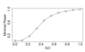
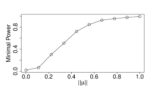
Figure 2: Two power plots for the minimal power of the test $\psi$ given a value for the norm $\|\mu\|$. The left panel is for a Sobolev ellipse with $\alpha=.5$, while the right panel is for $\alpha=1$. Both plots show the steadily increasing power of the minimax optimal test, and the ellipse with $\alpha=1$ appears to be slightly easier than the one with $\alpha=.5$.

4 Discussion

For completeness we would like to mention that if the set $K$ is a rotation of a QCO set, say $K=UK^{\prime}$ where $U$ is an orthogonal matrix, i.e., $U{{}^{\mathrm{\scriptscriptstyle T}}}U=\mathbbm{I}$, then one can transform the data by looking at $U{{}^{\mathrm{\scriptscriptstyle T}}}X$ and solve the corresponding QCO problem since $U{{}^{\mathrm{\scriptscriptstyle T}}}X=U{{}^{\mathrm{\scriptscriptstyle T}}}\mu+U{{}^{\mathrm{\scriptscriptstyle T}}}\xi$, where $U{{}^{\mathrm{\scriptscriptstyle T}}}\xi\sim N(0,\sigma^{2}\mathbb{I})$ and $U{{}^{\mathrm{\scriptscriptstyle T}}}\mu\in K^{\prime}$.

The result we developed in Section 2, should be compared and contrasted to the known result for the estimation problem. In detail, in the estimation problem one has $X_{i}=\mu_{i}+\xi_{i}$ for $i\in I$, where $\xi_{i}\sim N(0,\sigma^{2})$ are i.i.d., and one aims to estimate the vector $\mu$. Donoho et al., (1990) and Neykov, (2022) contain the minimax rate for this problem where $K$ is QCO for the $\ell_{2}$ and $\mathbb{R}^{n}$ case respectively. It turns out that the minimax rate for estimation, i.e., the rate of the following expression

$$\inf_{\widehat{\nu}}\sup_{\mu\in K}\mathbb{E}_{\mu}\|\widehat{\nu}(X)-\mu\|_{2}^{2},$$

is given by $(k^{*}+1)\sigma^{2}\wedge d^{2}_{0}(K)$ where $k^{*}\in I$ is such that $d_{k^{*}}(K)\leq\sqrt{k^{*}+1}\sigma$ and $d_{k^{*}-1}(K)\geq\sqrt{k^{*}}\sigma$. Note that for $j\in I$ such that $(j+1)\geq(k^{*}+1)^{2}$ we have $d_{j}(K)\leq d_{k^{*}}(K)\leq\sqrt{k^{*}+1}\sigma\leq\sqrt[4]{j+1}\sigma$, and thus $j\geq j^{*}$. It follows that $(j^{*}+1)\leq(k^{*}+1)^{2}$, and thus the minimax rate for testing is always better than that for estimation over QCO sets.

4.1 Open Problems

An exciting open problem is studying the localized minimax testing rates for QCO sets. A first step towards this was done by Wei and Wainwright, (2020), where the authors studied local testing rates in ellipsoids. It will be interesting to see how much of their results are generalizable to the QCO set setting. Furthermore, intuitively, the zero point looks like the worst point from a testing perspective for QCO constrained sets (as it possibly contains the largest local volume around itself compared to other points), hence it will be interesting to see whether the global minimax testing rate coincides with the ones that we derived in this paper.

Another avenue for future research will be to study different separation norms, i.e., instead of considering $\ell_{2}$ norm separation one can consider general $\ell_{q}$ norm separation for $q\geq 1$. It is unclear to us at the moment whether the Kolmogorov widths will still drive the minimax rate in that case.

Finally a more ambitious open problem is characterizing the minimax testing rates over general convex sets (containing the zero point). It will be quite exciting if one can show that there exists an optimal test for any convex set $K$, just as Neykov, (2022) showed that in the counterpart estimation problem there exists an optimal general estimating scheme that works for arbitrary convex sets.

A Deferred Proofs

Proof of Lemma 3.1.

Since $T^{\prime}\leq Z$ we have

$$\mathbb{P}(T^{\prime}\geq 2\sqrt{\alpha^{-1}}\sigma^{2}\sqrt{k})\leq\mathbb{P}(Z\geq 2C\sigma^{2}\sqrt{k})\leq\alpha,$$

which implies that the type I error of the test is controlled below the $\alpha$-level.

For the alternative we will use the Paley-Zygmund inequality. For a fixed $\theta$ we have

$$\mathbb{P}(T^{\prime}\geq\theta\mathbb{E}T^{\prime})\geq\frac{(1-\theta)^{2}(\mathbb{E}T^{\prime})^{2}}{\mathbb{E}T^{{}^{\prime}2}}.$$

Now $\mathbb{E}T^{\prime}\geq\mathbb{E}Z^{\prime}=\|P_{k}^{*}\mu\|^{2}_{2}$. On the other hand

$$\mathbb{E}T^{{}^{\prime}2} \leq\mathbb{E}Z^{2}=\mathbb{E}(\|P_{k}^{*}\mu\|^{2}_{2}+(P_{k}^{*}\mu){{}^{\mathrm{\scriptscriptstyle T}}}(\xi+\eta)+\xi{{}^{\mathrm{\scriptscriptstyle T}}}P_{k}^{*}\eta)^{2}$$

$$=\|P_{k}^{*}\mu\|^{4}_{2}+\|P_{k}^{*}\mu\|^{2}_{2}\sigma^{2}+4\sigma^{4}k+2\mathbb{E}(P_{k}^{*}\mu){{}^{\mathrm{\scriptscriptstyle T}}}(\xi+\eta)\xi{{}^{\mathrm{\scriptscriptstyle T}}}P_{k}^{*}\eta$$

$$\leq\|P_{k}^{*}\mu\|^{4}_{2}+\|P_{k}^{*}\mu\|^{2}_{2}\sigma^{2}+4\sigma^{2}k+4\|P_{k}^{*}\mu\|\sigma^{3}\sqrt{k}$$

where we used (2.3) and applied Cauchy-Schwartz in the last inequality. We conclude that

$$\mathbb{P}(T^{\prime}\geq\theta C\sqrt{k}\sigma^{2})\geq\mathbb{P}(T^{\prime}\geq\theta\|P_{k}^{*}\mu\|^{2}_{2}) \geq\mathbb{P}(T^{\prime}\geq\theta\mathbb{E}T^{\prime})$$

$$\geq\frac{(1-\theta)^{2}\|P_{k}^{*}\mu\|^{4}_{2}}{\|P_{k}^{*}\mu\|^{4}_{2}+\|P_{k}^{*}\mu\|^{2}_{2}\sigma^{2}+4\sigma^{2}k+4\|P_{k}^{*}\mu\|_{2}\sigma^{2}\sqrt{k}},$$ (A.1)

where the first bound follows since $\|P_{k}^{*}\mu\|^{2}_{2}=\|\mu\|^{2}_{2}-\|P_{k}^{*}\mu-\mu\|^{2}_{2}\geq\rho^{2}-d^{2}_{k}(K)\geq C\sqrt{k}\sigma^{2}$. A simple calculation shows that the map $x\mapsto\frac{x^{4}}{x^{4}+x^{2}\sigma^{2}+4\sigma^{2}k+4x\sigma^{2}\sqrt{k}}$ is an increasing function for $x\geq 0$. Plugging in this lower bound in (A) shows that at the expense of making $C$ “large” and $\theta$ “small” while still having $\theta C>2\sqrt{\alpha^{-1}}$ (i.e. select $\theta=4\sqrt{\alpha^{-1}}/C$ and take $C$ large) the probability on the right hand side of (A) can be made arbitrarily large. This completes the proof. ∎

Proof of Lemma 3.2.

The proof is based on a simple stochastic dominance argument. Let $\mu\in K$. The test statistic defined in Section 2.2 is given by

$$XP_{k}^{*}Y=[\|P_{k}^{*}(X+Y)\|^{2}_{2}-\|P_{k}^{*}(X-Y)\|^{2}_{2}]/4.$$

Observe that this is a difference of two independent random variables from the properties of the normal distribution. In addition $\|P_{k}^{*}(X+Y)\|^{2}_{2}$ is a $4\sigma^{2}$ times a non-central chi-squared random variable, with non-centralility parameter equal to $\lambda:=\|P_{k}^{*}\mu\|^{2}_{2}/(4\sigma^{2})$ and $k$-degrees of freedom. The cdf of a non-central chi-squared random variable is given by $1-Q_{k/2}(\sqrt{\lambda},\sqrt{x})$ where $Q$ is the Marcum Q-funciton. It is known that the Marcum Q-function is increasing in $\lambda$ for all $x,k>0$ (Sun et al.,, 2010) which implies that $\|P_{k}^{*}(X+Y)\|^{2}_{2}$ stochastically dominates $\|P_{k}^{*}(X^{\prime}+Y^{\prime})\|^{2}_{2}$ where $X^{\prime}=\mu^{\prime}+\xi$, $Y^{\prime}=\mu^{\prime}+\eta$ where $\|P_{k}\mu^{\prime}\|_{2}\leq\|P_{k}\mu\|_{2}$. Since the variables $\|P_{k}^{*}(X-Y)\|^{2}_{2}\stackrel{{\scriptstyle d}}{{=}}\|P_{k}^{*}(X^{\prime}-Y^{\prime})\|^{2}_{2}$ and are independent of $\|P_{k}^{*}(X+Y)\|^{2}_{2},\|P_{k}^{*}(X^{\prime}+Y^{\prime})\|^{2}_{2}$ we can claim that $XP_{k}^{*}Y$ stochastically dominates $X^{\prime}P_{k}^{*}Y^{\prime}$. The final implication is because the function $z\mapsto\mathbbm{1}(z_{+}\geq c)$ is increasing for any $c\in\mathbb{R}$, and by first order stochastic dominance we know that the expectation of any increasing function satisfies

$$\mathbb{E}\mathbbm{1}((XP_{k}^{*}Y)_{+}\geq c)\geq\mathbb{E}\mathbbm{1}((X^{\prime}P_{k}^{*}Y^{\prime})_{+}\geq c),$$

whenever $\|P_{k}^{*}\mu\|_{2}\geq\|P_{k}^{*}\mu^{\prime}\|_{2}$. ∎

Proof of Lemma 3.3.

If $k=n$ the assertion is obvious since $\|P_{k}^{*}\mu\|_{2}=\|\mu\|_{2}=\sqrt{c}$ which is achieved at the vector given in the statement of the lemma. If $c<a_{n-k}$, then the vector

$$\mu=(\underbrace{0,\ldots,0}_{n-k-1},\sqrt{c},0,\ldots,0)\in K$$

and furthermore $\|P^{*}_{k}\mu\|_{2}=0$ so the assertion is once again obivous. Let us now assume that $c\geq a_{n-k}$ and $k<n$. We have that $\sum_{i=1}^{n}\mu_{i}^{2}=c$. Hence $\sum_{i=1}^{n-k}\mu_{i}^{2}=c-\sum_{i=n-k+1}^{n}\mu_{i}^{2}$. On the other hand since $\sum_{i=1}^{n}\mu^{2}_{i}/a_{i}\leq 1$ and $\{a_{i}\}_{i\in[n]}$ form an increasing sequence, we have

$$\frac{c-\sum_{i=n-k+1}^{n}\mu_{i}^{2}}{a_{n-k}}\leq\sum_{i=1}^{n-k}\mu_{i}^{2}/a_{i}\leq 1-\sum_{i=n-k+1}^{n}\mu_{i}^{2}/a_{i}$$

Rearranging gives

$$c/a_{n-k}-1\leq\sum_{i=n-k+1}^{n}\mu_{i}^{2}(1/a_{n-k}-1/a_{i})\leq\sum_{i=n-k+1}^{n}\mu_{i}^{2}(1/a_{n-k}-1/a_{n}),$$

and we conclude that $\|P_{k}^{*}\mu\|^{2}_{2}=\sum_{i=n-k+1}^{n}\mu_{i}^{2}\geq\frac{c/a_{n-k}-1}{1/a_{n-k}-1/a_{n}}$. It is clear that the vector given in the lemma statement achieves this bound. The only thing it remains to see is that this vector indeed has norm $c$ and it belongs to $K$. Simple algebra verifies this and completes the proof. ∎

References

• Baraud, (2002) Baraud, Y. (2002). Non-asymptotic minimax rates of testing in signal detection. Bernoulli, pages 577–606.
• Carbery and Wright, (2001) Carbery, A. and Wright, J. (2001). Distributional and ${L}^{q}$ norm inequalities for polynomials over convex bodies in $\mathbb{R}^{n}$. Mathematical research letters, 8(3):233–248.
• Diakonikolas et al., (2022) Diakonikolas, I., Kane, D. M., and Pensia, A. (2022). Gaussian mean testing made simple. arXiv preprint arXiv:2210.13706.
• Donoho et al., (1990) Donoho, D. L., Liu, R. C., and MacGibbon, B. (1990). Minimax risk over hyperrectangles, and implications. The Annals of Statistics, pages 1416–1437.
• Ermakov, (1991) Ermakov, M. S. (1991). Minimax detection of a signal in a gaussian white noise. Theory of Probability & Its Applications, 35(4):667–679.
• Ingster and Suslina, (2003) Ingster, Y. and Suslina, I. (2003). Nonparametric goodness-of-fit testing under Gaussian models, volume 169. Springer Science & Business Media.
• Ingster, (1982) Ingster, Y. I. (1982). On the minimax nonparametric detection of signals in white gaussian noise. Problemy Peredachi Informatsii, 18(2):61–73.
• (8) Ingster, Y. I. (1993a). Asymptotically minimax hypothesis testing for nonparametric alternatives. I. Math. Methods Statist, 2(2):85–114.
• (9) Ingster, Y. I. (1993b). Asymptotically minimax hypothesis testing for nonparametric alternatives. II. Math. Methods Statist, 3(2):171–189.
• (10) Ingster, Y. I. (1993c). Asymptotically minimax hypothesis testing for nonparametric alternatives. III. Math. Methods Statist, 4(2):249–268.
• Ingster and Suslina, (2000) Ingster, Y. I. and Suslina, I. A. (2000). Minimax nonparametric hypothesis testing for ellipsoids and besov bodies. ESAIM: Probability and Statistics, 4:53–135.
• Johnstone, (2019) Johnstone, I. M. (2019). Gaussian estimation: Sequence and wavelet models. Unpublished manuscript.
• Neykov, (2022) Neykov, M. (2022). On the minimax rate of the gaussian sequence model under bounded convex constraints. arXiv preprint arXiv:2201.07329.
• Pinkus, (2012) Pinkus, A. (2012). N-widths in Approximation Theory, volume 7. Springer Science & Business Media.
• Sun et al., (2010) Sun, Y., Baricz, Á., and Zhou, S. (2010). On the monotonicity, log-concavity, and tight bounds of the generalized marcum and nuttall $q$-functions. IEEE Transactions on Information Theory, 56(3):1166–1186.
• Suslina, (1996) Suslina, I. (1996). Minimax signal detection forl q-ellipsoids withl p-balls removed. Journal of Mathematical Sciences, 81(1):2442–2449.
• Tsybakov, (2009) Tsybakov, A. B. (2009). Introduction to Nonparametric Estimation. Springer.
• Wainwright, (2019) Wainwright, M. J. (2019). High-dimensional statistics: A non-asymptotic viewpoint, volume 48. Cambridge University Press.
• Wei et al., (2020) Wei, Y., Fang, B., and Wainwright, M. J. (2020). From gauss to kolmogorov: Localized measures of complexity for ellipses. Electronic Journal of Statistics, 14(2):2988–3031.
• Wei and Wainwright, (2020) Wei, Y. and Wainwright, M. J. (2020). The local geometry of testing in ellipses: Tight control via localized kolmogorov widths. IEEE Transactions on Information Theory, 66(8):5110–5129.