A Strength and Sparsity Preserving Algorithm for Generating Weighted, Directed Networks with Predetermined Assortativity

Abstract

Degree-preserving rewiring is a widely used technique for generating unweighted networks with given assortativity, but for weighted networks, it is unclear how an analog would preserve the strengths and other critical network features such as sparsity level. This study introduces a novel approach for rewiring weighted networks to achieve desired directed assortativity. The method utilizes a mixed integer programming framework to establish a target network with predetermined assortativity coefficients, followed by an efficient rewiring algorithm termed “strength and sparsity preserving rewiring” (SSPR). SSPR retains the node strength distributions and network sparsity after rewiring. It is also possible to accommodate additional properties like edge weight distribution with extra computational cost. The optimization scheme can be used to determine feasible assortativity ranges for an initial network. The effectiveness of the proposed SSPR algorithm is demonstrated through its application to two classes of popular network models.

Key words. attainable assortativity, directed assortativity, mixed integer programming, weighted network rewiring

1 Introduction

Assortativity is an important measure characterizing the correlation structure of nodal features of networks. Generating random networks with predetermined assortativity is critical for justifying network theories (Newman, 2003), exploring spectral properties (Van Mieghem et al., 2010), improving model fit (Wang et al., 2022), and optimizing network robustness (Chan and Akoglu, 2016). Edge rewiring is a widely accepted technique for generating networks with given assortativity. The degree-preserving rewiring (DPR) algorithm proposed by Newman (2003) ensures that the node degree distribution of an undirected network keeps unchanged throughout the course of rewiring so as to preserve the fundamental topology of the rewired network. An extension of Newman’s algorithm, called DiDPR, was recently developed for generating directed networks with predetermined directed assortativity coefficients (Wang et al., 2022). More generally, rewiring techniques have found practical applications in many fields such as biological science (Iorio et al., 2016), clinical trials (Staples et al., 2015), and social network analysis (Schweimer et al., 2022), among others.

Despite the long availability of Newman’s algorithm for unweighted networks, rewiring a weighted network to achieve predetermined assortativity proves to be a challenging task that has not yet been studied in the literature. While directly extending Newman’s algorithm to weighted networks may seem feasible for preserving node strengths, a naive extension fails to retain other important network properties, such as sparsity, simultaneously. When edge weights are represented as integer values, one potential approach involves a multi-edge scheme, where a weighted edge is divided into multiple unit-weight edges, and then Newman’s two-swap method or similar techniques are applied. However, this approach does not translate smoothly to networks with real-valued edge weights. Even for networks with integer-valued edge weights, this method lacks practical utility, as it results in a substantial increase in the number of edges (Wuellner et al., 2010) and alters the network’s sparsity, a typical feature observed in most real-world networks (Barabási, 2016). In the subsequent section, we will delve into more details about this approach and explore other potential possibilities for addressing the challenge of rewiring weighted networks to achieve predetermined assortativity.

This paper introduces a novel rewiring algorithm for generating weighted, directed networks with four predetermined directed assortativity coefficients (Yuan et al., 2021). Notably, the proposed algorithm ensures that both out- and in-strength distributions, along with sparsity, are meticulously preserved upon the completion of the rewiring process. Newman’s approach involves searching for a target network structure characterized by a joint degree distribution that matches the desired assortativity values and represents the stationary status of the rewiring process (Newman, 2003; Wang et al., 2022). In contrast, the proposed algorithm directly produces a weighted, directed network with assortativity measures precisely equal to the given values, provided that they are attainable. The desired network structure is not unique and we formulate an optimization problem to provide one feasible solution. With carefully chosen objective function for the optimization, the algorithm can retain certain network topology and properties in addition to strength distributions and sparsity after rewiring. Further, the optimization scheme also helps to identify the attainability of each assortativity coefficient by establishing its upper and lower bounds given the initial network configuration.

The remainder of the paper is organized as follows. Section 2 introduces the notations and elucidates the challenges for the extension of Newman’s algorithm to weighted networks. Section 3 presents an efficient strength and sparsity preserving reserving algorithm for weighted, directed networks with given assortativity coefficients, followed by an approach to determining assortativity coefficient bounds and a generalization allowing to consider other network properties like edge weight distribution. Section 4 provides extensive simulations showing the applications of the proposed algorithm to the Erdös-Rényi model and the Barabási-Albert model. Lastly, some discussions and future works are addressed in Section 5.

2 Preliminaries

Starting with notations, we layout the challenges when extending Newman’s algorithm to weighted, directed networks.

2.1 Notations

Let $G:=G(V,E)$ be a weighted, directed network with node set $V$ and edge set $E$. Additionally, let $(v_{i},v_{j},w_{ij})\in E$ denote a weighted, directed edge from source node $v_{i}\in V$ to target node $v_{j}\in V$ with weight $w_{ij}>0$. For the special case of $v_{i}=v_{j}$, $(v_{i},v_{j},w_{ij})\in E$ is a self-loop. Network $G$ is characterized by its associated adjacency matrix $\bm{W}:=(w_{ij})_{n\times n}$, where $n=|V|$ is the number of nodes in $G$. If there is no edge from $v_{i}$ to $v_{j}$, i.e., $(v_{i},v_{j},w_{ij})\notin E$, then the corresponding $w_{ij}$ in $\bm{W}$ is set to $0$. Fundamental node-level properties of weighted, directed networks are $s^{\,(1)}_{i}:=\sum_{v_{j}\in V}w_{ij}$ and $s^{\,(2)}_{i}:=\sum_{v_{j}\in V}w_{ji}$, which respectively refer to the out- and in-strength of node $v_{i}$. The superscripts “$1$” and “$2$” are respectively used to represent “out” and “in” throughout the rest of the manuscript for simplicity.

The directed assortativity coefficients considered in this paper are adopted from those proposed by Yuan et al. (2021). By considering the combinations of out- and in-strengths of source and target nodes, there are four types of assortativity coefficients, denoted by $r(a,b)=r_{\bm{W}}(a,b)$ with $a,b\in\{1,2\}$, where $r(a,b)$ is the assortativity coefficient based on the $a$-strength of source nodes and $b$-strength of target nodes. For example, $r(1,2)$ refers to the assortativity coefficient based on the out-strength of source nodes and in-strength of target nodes. The rest three are interpreted in the similar manner.

Mathematically, the directed assortativity coefficients are expressed as

$$r(a,b)=\frac{\sum_{v_{i},v_{j}\in V}w_{ij}\left[\left(s_{i}^{(a)}-\bar{s}_{\rm src}^{\,(a)}\right)\left(s_{j}^{(b)}-\bar{s}_{\rm trg}^{\,(b)}\right)\right]}{\tau\sigma_{\rm src}^{(a)}\sigma_{\rm trg}^{(b)}},\qquad a,b\in\left\{1,2\right\},$$ (1)

where $\tau:=\sum_{v_{i},v_{j}\in V}w_{ij}$ is the total weight of all edges,

$$\bar{s}_{\rm src}^{\,(a)}:=\frac{\sum_{v_{i},v_{j}\in V}w_{ij}s_{i}^{\,(a)}}{\tau}=\frac{\sum_{v_{i}\in V}s^{\,(1)}_{i}s_{i}^{\,(a)}}{\tau}$$

is the weighted mean of the $a$-type strength of source nodes and

$$\sigma_{\rm src}^{\,(a)}:=\sqrt{\frac{\sum_{v_{i},v_{j}\in V}w_{ij}\left(s_{i}^{\,(a)}-\bar{s}_{\rm src}^{\,(a)}\right)^{2}}{\tau}}=\sqrt{\frac{\sum_{v_{i}\in V}s^{\,(1)}_{i}\left(s_{i}^{\,(a)}-\bar{s}_{\rm src}^{\,(a)}\right)^{2}}{\tau}}$$

is the associated weighted standard deviation. The counterparts $\bar{s}_{\rm trg}^{\,(b)}$ and $\sigma_{\rm trg}^{\,(b)}$ are defined analogously for target nodes. For more properties about the directed, weighted assortativity coefficients, see Yuan et al. (2021).

2.2 Challenges

Newman’s algorithm for generating an unweighted, undirected network with a predetermined assortativity measure is based on a two-swap DPR algorithm (Newman, 2003). It effectively adjusts the assortativity while preserving the marginal node degree distribution. Recently, this idea was translated into a practical approach with concrete via a convex optimization framework, and further extended to unweighted, directed networks by Wang et al. (2022). The extension solely requires accounting for edge directions during the rewiring process, and since all edges possess unit weight, both node degrees and the total edge number remain unchanged. For a graphical illustration, refer to the top-left panel of Figure 1.

Figure 1: Top-left panel: An illustration of DPR in Newman (2003) and DiDPR in Wang et al. (2022); Dashed edges refer to the edges that are removed in the rewiring; Each edge has weight $1$. Top-right panel: An illustration of DPR directly extended to weighted, directed networks; Edge weights are given next to the corresponding edges. Bottom panel: An illustration of three-swap rewiring for weighted, directed networks.

An example that attempts to extend Newman’s algorithm to a weighted, directed network (Wuellner et al., 2010) is shown in the top-right panel of Figure 1. As depicted, however, when the sampled edges for swap have different weights, an additional edge with weight equal to their weight difference needs to be added to preserve node strengths; the rightmost red edge (with weight $2$) from $v_{2}$ to $v_{4}$ illustrates this necessity. Consequently, this attempt becomes impractical, as it leads to a significant increase in the number of edges during the rewiring process, thereby compromising network sparsity. For certain special cases, a potential remedy is to generalize the three-swap idea introduced by Uribe-Leon et al. (2020). The bottom panel of Figure 1 demonstrates an example of this approach, which is applicable only to simple edge weights (e.g., integer-valued) and demands additional efforts to search specific structures for rewiring to occur. In the provided example, it requires sampling a module of four nodes connected by three directed edges, where the out-strengths of the source nodes (i.e., $v_{1}$ and $v_{2}$) are identical. Candidate structures satisfying such restrictions may be scarce or non-existent, making methods based on three-swap impractical in real-world scenarios.

Furthermore, an issue not investigated by Newman (2003) is whether the predetermined assortativity level is achievable through rewiring. Newman’s algorithm requires the development of a transition matrix $\bm{M}$ to construct the joint edge degree distribution for the target network with predetermined assortativity. The existence of this matrix $\bm{M}$ is not guaranteed as it depends on both the structure of the initial network and the predetermined assortativity value. In other words, given an initial network, not every predetermined assortativity level is attainable through rewiring. Inspired by the work of Wang et al. (2022), as a byproduct, this paper also delves into an investigation of assortativity attainability by determining upper and lower bounds for each of the four directed assortativity coefficients, conditional on the structure of the initial network.

3 Strength and Sparsity Preserving Rewiring

We propose an efficient strength and sparsity preserving rewiring (SSPR) algorithm designed for weighted, directed networks with predetermined assortativity coefficients. The crux of the algorithm lies in the quest for a target network with the desired assortativity coefficients by solving a mixed integer linear programming problem. Subsequently, the algorithm employs a novel rewiring technique to ensure the preservation of critical network properties, such as marginal strength distributions and network sparsity. the rewiring process.

3.1 Finding a Target Network

Given a fully observed network $G:=G(V(G),E(G))$ with a weighted adjacency matrix $\bm{W}$ and predetermined assortativity measures $r^{*}(a,b),a,b\in\left\{1,2\right\}$, the primary goal is to generate a new network $H$ (defined on the same node set $V(H)=V(G)=V$, but with a different edge set $E(H)\neq E(G)$) whose assortativity measures are equal to the given $r^{*}(a,b)$ through rewiring $G$. Meanwhile, it is essential to retain crucial network properties like node out- and in-strength distributions and network sparsity after rewiring. Provided that such $H$ exists, its adjacency matrix $\bm{\Lambda}:=(\lambda_{ij})_{n\times n}$, which is referred to as the target adjacency matrix, must satisfy the following conditions:

1. The entries of $\bm{\Lambda}$ are non-negative, i.e., $\lambda_{ij}\geq 0$ for all $v_{i},v_{j}\in V$;

2. The row and column sums of $\bm{\Lambda}$ are identical to the counterparts in $\bm{W}$ (preserving marginal strength distributions);

3. The number of non-zero elements in $\bm{\Lambda}$ is the same as that in $\bm{W}$ (preserving network sparsity);

4. The assortativity measures (of $\bm{\Lambda}$) computed from Equation (1) are equal to the given $r^{*}(a,b)$ for all $a,b\in\{1,2\}$.

Depending on the analytic objectives and computing resources, one may also include additional conditions that restrict the lower and upper bounds of the non-zero elements in $\bm{\Lambda}$ in order to prevent the emergence of a large proportion of extremely small weights or unexpected outliers.

Now the problem boils down to finding a suitable target adjacency matrix $\bm{\Lambda}$, which may not be unique, but any single solution would suffice. To set it up, consider a latent, binary matrix $\bm{Z}:=(z_{ij})_{n\times n}$ associated with $\bm{\Lambda}$, where $z_{ij}=1$ for $\lambda_{ij}>0$; $z_{ij}=0$ otherwise. The search for a solution to $\bm{\Lambda}$ involves solving a mixed integer linear programming problem as follows:

$$\min_{\bm{\Lambda}}\quad f(\bm{\Lambda}),$$

s.t. $$\lambda_{ij}=0\textrm{ if }z_{ij}=0,\quad\forall v_{i},v_{j}\in V,$$

$$\kappa_{\rm L}\leq\lambda_{ij}\leq\kappa_{\rm U}\textrm{ if }z_{ij}=1,\quad\forall v_{i},v_{j}\in V,$$

$$\sum_{i,j}z_{ij}=|E(G)|,$$

$$\sum_{i}\lambda_{ij}=\sum_{i}w_{ij}=s^{\,(2)}_{j},\quad\forall v_{j}\in V,$$

$$\sum_{j}\lambda_{ij}=\sum_{j}w_{ij}=s^{\,(1)}_{i},\quad\forall v_{i}\in V,$$

$$r_{\bm{\Lambda}}(a,b)=r^{*}(a,b),\quad a,b\in\{1,2\},$$

where $\kappa_{\rm U}\geq\kappa_{\rm L}>0$ are the preset upper and lower bounds for edge weights, and $f(\cdot)$ is an arbitrary linear function.

In theory, the objective function $f(\cdot)$ can be any function of $\bm{\Lambda}$ and the constraints do not have to be linear in $\bm{\Lambda}$. For instance, one may set $f(\bm{\Lambda})=\sum_{i,j}|w_{ij}-\lambda_{ij}|$ if it is desired that the edge weight distribution changes as little as possible after rewiring. Nonetheless, the more complex the objective function is and the more additional constraints are, the more time is required for solving the optimization problem even with a possibility of unsolvable risks. Especially when there are non-linear constraints, the optimization problem becomes a mixed integer non-linear programming problem, which demands more solving time or even computationally intractable. Therefore, when there is no mandatory condition for $f(\cdot)$, we recommend setting it to zero for improving the optimization speed. Mathematical programming solvers like Gurobi (Gurobi Optimization, LLC, 2023) and CPLEX (IBM, 2022) can be used to efficiently solve such problems.

A byproduct of the optimization scheme is that it can be used to determine the bounds of feasible assortativity levels. Given an initial network $G$, not all the values in the natural bounds of assortativity coefficient (i.e., $[-1,1]$) are attainable through SSPR that will be elaborated in the next subsection. From Equation (1), the assortativity coefficients are linear in edge weights, allowing us to find the assortativity bounds by adjusting the objective function. Specifically, we can set the objective function to be $f(\bm{\Lambda})=\sum_{i,j}\lambda_{ij}s_{i}^{(a)}s_{j}^{(b)}$ to find the lower bound of $r^{*}(a,b)$, and set $f(\bm{\Lambda})=-\sum_{i,j}\lambda_{ij}s_{i}^{(a)}s_{j}^{(b)}$ to find the upper bound of $r^{*}(a,b)$. See detailed illustrations in Section 4.

3.2 Rewiring towards Target Network

Once the target adjacency matrix $\bm{\Lambda}$ is determined, the next crucial task is to establish a feasible rewiring scheme to move from given $\bm{W}$ towards $\bm{\Lambda}$ while preserving node in- and out-strengths and network sparsity. Figure 2 shows a hypothetical example of rewiring a pair of edges $(v_{i},v_{j},w_{ij})$ and $(v_{k},v_{l},w_{kl})$ among four nodes $v_{i}$, $v_{j}$, $v_{k}$ and $v_{l}$. The underlying principle is to keep the out- and in-strengths of the four nodes identical by a meticulously redistributed weight of amount $\Delta w\leq\min\{w_{ij},w_{kl}\}$. It is worth noting that the directed edges $(v_{k},v_{j},w_{kj})$ and $(v_{i},v_{l},w_{il})$ may not exist before rewiring, and that the selected edges $(v_{i},v_{j},w_{ij})$ and $(v_{k},v_{l},w_{kl})$ may be removed after rewiring, so represented by dotted lines. The corresponding changes in the adjacency matrix are illustrated in the lower panel of Figure 2. It is clear that the row and column sums in the adjacency matrix remain unchanged. An appropriate $\Delta w$ must be determined for each rewiring step.

$$\begin{pmatrix}\cdots&\vdots&\cdots&\vdots&\cdots\\ \cdots&w_{ij}&\cdots&w_{il}&\cdots\\ \cdots&\vdots&\cdots&\vdots&\cdots\\ \cdots&w_{kj}&\cdots&w_{kl}&\cdots\\ \cdots&\vdots&\cdots&\vdots&\cdots\\ \end{pmatrix}\Longrightarrow\begin{pmatrix}\cdots&\vdots&\cdots&\vdots&\cdots\\ \cdots&w_{ij}-\Delta w&\cdots&w_{il}+\Delta w&\cdots\\ \cdots&\vdots&\cdots&\vdots&\cdots\\ \cdots&w_{kj}+\Delta w&\cdots&w_{kl}-\Delta w&\cdots\\ \cdots&\vdots&\cdots&\vdots&\cdots\\ \end{pmatrix}$$

Figure 2: A hypothetical example reflecting the principle of rewiring through a graphical representation and the corresponding changes in the adjacency matrix.

Before proceeding, however, it is crucial to show the existence of at least one rewiring path from $\bm{W}$ to $\bm{\Lambda}$. To achieve this, define $\bm{\Psi}:=(\psi_{ij})_{n\times n}=\bm{W}-\bm{\Lambda}$, the difference between the initial adjacency matrix $\bm{W}$ and the target adjacency matrix $\bm{\Lambda}$. A successful rewiring process means that, at the end of the rewiring, $\psi_{ij}=0$ for all $i,j\in\{1,\ldots,n\}$. We employ a sweeping procedure to adjust all $\psi_{ij}$’s one by one in an order from the top to the bottom and the left to the right within each row. The existence of a path is shown by induction. Suppose that $\psi_{ij}$ is the next element in the sweeping procedure awaiting an adjustment via rewiring. That is, we already have $\psi_{kl}=0$ for all $l$ if $k<i$ and for $l<j$ if $k=i$ from previous sweeping steps. Proposition 3.1 shows the existence of a rewiring path leading to $\psi_{ij}=0$ with the associated proof given in Appendix A.

Proposition 3.1.

For any $i,j<n$, there always exists a path leading to $\psi_{ij}=0$ after rewiring.

$$\begin{pmatrix}0&0&0&0\\ 0&{\color[rgb]{0,0,1}3}&-2&-1\\ 1&-1&{\color[rgb]{1,0,0}2}&-2\\ -1&-2&0&{\color[rgb]{1,0,0}3}\end{pmatrix}\overset{\Delta w=2}{\Longrightarrow}\begin{pmatrix}0&0&0&0\\ 0&{\color[rgb]{0,0,1}1}&0&-1\\ 1&1&{\color[rgb]{1,0,0}0}&-2\\ -1&-2&0&{\color[rgb]{1,0,0}3}\end{pmatrix}\overset{\Delta w=1}{\Longrightarrow}\begin{pmatrix}0&0&0&0\\ 0&{\color[rgb]{0,0,1}0}&0&0\\ 1&1&{\color[rgb]{1,0,0}0}&-2\\ -1&-1&0&{\color[rgb]{1,0,0}2}\end{pmatrix}.$$

Figure 3: An example of rewiring scheme illustrating Proposition 3.1.

Figure 3 illustrates an example of a rewiring scheme corresponding to the principle behind Proposition 3.1. The objective is to transform $\psi_{22}=3$ (shown in blue) to $0$ through rewiring. The $\psi_{i^{\ast}j^{\ast}}$’s to be adjusted are highlighted in red, with the corresponding $\Delta w$ values indicated above the arrows. Notably, the selection of $\Delta w$ values is not unique. To reduce subsequent rewiring steps, we prioritize making non-sweeped $\psi_{ij}$’s zero whenever possible. Specifically, for each pair $(k,l)$ with $k>i$ and $l>j$, given $\psi_{ij}>0$, we set $\Delta w=\min\{\psi_{ij},\max\{\psi_{kl},0\}\}$; given $\psi_{ij}<0$, we set $\Delta w=\max\{\psi_{ij},\min\{-\psi_{kj},0\},\min\{-\psi_{il},0\}\}$. These additional conditions for $\Delta w$ selection are essential to prevent the generation of negative edge weights during the rewiring process.

Input: Initial adjacency matrix $\bm{W}$;
target adjacency matrix $\bm{\Lambda}$.

Output: Rewiring record $R$.

Algorithm :

       $n\leftarrow$ number of rows (or columns) of $\bm{W}$;

       Initialize an empty list of rewiring steps $R$;

       $\bm{\Psi}\leftarrow\bm{W}-\bm{\Lambda}$;

       for $i=1$ to $n-1$ do

             /* Possibly insert a reorder step here to put elements with larger magnitude earlier */

             for $j=1$ to $n-1$ do

                   $\bm{\Psi},R\leftarrow$ Rewire($\bm{\Psi},R,i,j,n$);

                  

             end for

            

       end for

      return $R$;

      

Function Rewire:

       Input: Matrix $\bm{\Psi}$;
rewiring record $R$;
row and column indices $i$ and $j$;
number of rows $n$.

       Output: Updated $\bm{\Psi}$ and $R$.

       for $k=i+1$ to $n$ do

             for $l=j+1$ to $n$ do

                   if $\psi_{ij}>0$ then

                         $\Delta w\leftarrow\min(\psi_{ij},\max(0,\psi_{k,l}))$;

                        

                   else if $\psi_{ij}<0$ then

                         $\Delta w\leftarrow\max(\psi_{ij},\min(0,-\psi_{i,l}),\min(0,-\psi_{k,j}))$;

                        

                   if $\psi_{ij}==0$ or $\Delta w==0$ then

                         Continue to the next $l$;

                        

                   $\psi_{ij}\leftarrow\psi_{ij}-\Delta w$ ;

                    /* Update $\bm{\Psi}$ */

                   $\psi_{kl}\leftarrow\psi_{kl}-\Delta w$;

                   $\psi_{il}\leftarrow\psi_{il}+\Delta w$;

                   $\psi_{kj}\leftarrow\psi_{kj}+\Delta w$;

                   if $\Delta w>0$ then /* Record rewiring step */

                         Append $(i,j,k,l,\Delta w)$ to $R$;

                        

                   else

                         Append $(i,l,k,j,-\Delta w)$ to $R$;

                        

                  

             end for

            

       end for

      return $\bm{\Psi}$, $R$;

      

Algorithm 1 Pseudo codes of the SSRP algorithm.

The pseudo codes for the SSPR algorithm are summarized in Algorithm 1. Given the difference matrix $\bm{\Psi}$, the Rewire function sweeps through its elements one at a time. Note that the sweep only needs to be done for the first $n-1$ rows as the column sums are zero; similarly, within each row of $\bm{\Psi}$, we only need sweep the first $n-1$ elements as all the row sums are zero. At the beginning of each row, an optional step is to reorder the rows and columns so that elements with larger magnitude get sweeped earlier. This would reduce the number of rewiring steps (about 45% in our experiments in Section 4), but the extra sorting step would increase the time complexity of the algorithm. The output of Algorithm 1 is the list of entire rewiring history of $(i,j,k,l,\Delta w)$ for each step, where $i$, $j$, $k$, and $l$ are the indices of the selected nodes $v_{i}$, $v_{j}$, $v_{k}$, and $v_{l}$ for rewiring, and $\Delta w$ is the associated rewiring weight.

4 Simulations

We validate the proposed SSPR algorithm through simulation studies using two widely used network models: the Erdös-Rényi (ER) model (Erdös and Rényi, 1959; Gilbert, 1959) and the Barabási-Albert model, also known as the preferential attachment (PA) model (Barabási and Albert, 1999). Both models in their classic forms are unweighted, but, in our study, they are extended by incorporating edge directions and weights. The algorithm implementation is primarily based on the gurobipy module (Gurobi Optimization, LLC, 2023) in Python, and the program was run on AMD EPYC 7763 processors utilizing 4 threads and 8 GB of memory.

4.1 ER Network Model

The classic ER model is governed by two parameters: the number of nodes $n$ and the probability of emergence of a directed edge $p$. We augment the classic ER model by allowing self-loops (from a node to itself) and edge weights. Specifically, three levels of $n\in\{50,100,200\}$ and three levels of $p\in\{0.05,0.1,0.2\}$ were considered. Edge weights were generated from a gamma distribution with shape $5$ and scale $0.2$. For each configuration, a total of $100$ ER networks were generated. Isolated nodes, if any, were removed from the network prior to rewiring. Pertaining to the nature of the ER model, all of the four assortativity coefficients are expected to converge to $0$ for large $n$.

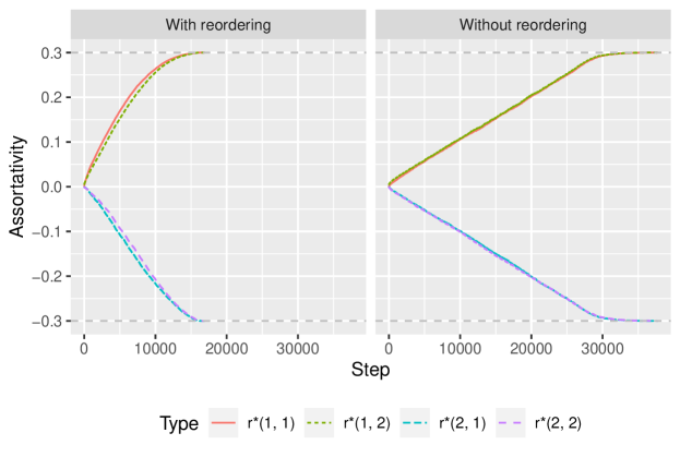
Figure 4: Average trace plots for $100$ replicates of ER networks with $n=200$, $p=0.1$, target assortativity coefficients set to $r^{*}(1,1)=r^{*}(1,2)=0.3$, $r^{*}(2,1)=r^{*}(2,2)=-0.3$, and objective function given by $f(\bm{\Lambda})=0$. The left panel shows the results with reordering, but the right panel shows those without reordering.

Figure 4 shows the results for $n=200$ and $p=0.1$ as an example. The results for other settings of $n$ and $p$ present a similar pattern, so they are omitted. The target assortativity coefficients were $r^{*}(1,1)=r^{*}(1,2)=0.3$, $r^{*}(2,1)=r^{*}(2,2)=-0.3$, and a simple objective function $f(\bm{\Lambda})=0$ was used to determine the target adjacency matrix for the assortativity coefficients. The left panel presents the results with the reordering procedure implemented, and the right panel presents the results without reordering. Each panel shows the average trace plots for the four assortativity coefficients during rewiring. We observe that all of the assortativity coefficients successfully reached their targets through the proposed SSPR algorithm, regardless of whether the reordering procedure was implemented. However, the right panel shows a significant increase in the number of rewiring steps when the reordering procedure was not executed into the SSPR algorithm.

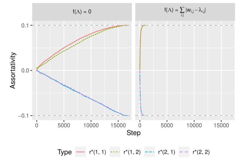
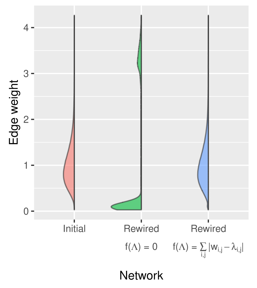
Figure 5: Average trace and edge weight violin plots for $100$ replicates of ER networks with $n=200$ and $p=0.1$, target assortativity coefficients set to $r^{*}(1,1)=r^{*}(1,2)=0.1$ and $r^{*}(2,1)=r^{*}(2,2)=-0.1$.

To illustrate the impact of the selection of objective function $f(\cdot)$, consider rewiring ER networks with $n=200$ and $p=0.1$ to achieve assortativity coefficients $r^{*}(1,1)=r^{*}(1,2)=0.1$ and $r^{*}(2,1)=r^{*}(2,2)=-0.1$. Two objective functions $f(\bm{\Lambda})=0$ and $f(\bm{\Lambda})=\sum_{i,j}|w_{ij}-\lambda_{ij}|$ were used in setting up the mixed integer programming problem in Section 3.1. The average trace plots of the assortativity levels based on $100$ simulated networks are displayed in the left two panels of Figure 5. Clearly, the algorithm with the more complex objective function $f(\bm{\Lambda})=\sum_{i,j}|w_{ij}-\lambda_{ij}|$ requires much fewer rewiring steps for the assortativity coefficients to reach the predetermined targets. The right panel of Figure 5 compares the density of the edge weights of the initial networks and the rewired networks obtained under the two objective functions. The post-rewiring edge weight distribution with objective function $f(\bm{\Lambda})=0$ is noticeably different from that of the initial networks. In contrast, the post-rewiring edge weight distribution with objective function $f(\bm{\Lambda})=\sum_{i,j}|w_{ij}-\lambda_{ij}|$ is almost identical to that of the initial networks.

The comparisons in Figure 5 seems suggesting a preference of using $f(\bm{\Lambda})=\sum_{i,j}|w_{ij}-\lambda_{ij}|$ as the objective function, but there are other factors to consider. Fewer rewiring steps do not necessarily mean less overall computation time. In fact, among the $100$ replicates in the present example, the median computation time for $f(\bm{\Lambda})=0$ was $5$ seconds, but for $f(\bm{\Lambda})=\sum_{i,j}|w_{ij}-\lambda_{ij}|$ it was about $191$ seconds. Further, there is no guarantee that optimization problem with the more complex objective function can be solved within a reasonable amount of time. For instance, for the experiment of ER networks with $n=100$ and $p=0.01$, $48$ out of the $100$ simulations did not finish within $12$ hours on a computer with AMD EPYC 7763 processors with 4 threads and 8 GB of RAM.

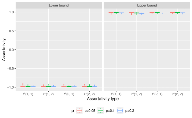
Figure 6: Side-by-side box plots for the upper and lower bounds of assortativity coefficients based on $100$ replicates of ER networks with $n=200$ and $p\in\{0.05,0.1,0.2\}$.

Figure 6 shows the box plots of the attainable upper and lower bounds of assortativity coefficients for the 100 ER networks generated under each combination of $n=200$ and $p\in\{0.05,0.1,0.2\}$. It appears that the bounds are very close to the nominal bounds of $-1$ and $1$. That is, all the values between $-1$ and $1$ appear to be attainable for all four assortativity coefficients. Such observation is expected owing to the feature of ER networks.

4.2 PA Network Model

Figure 7: The $\alpha$, $\beta$ and $\gamma$ edge-creation scenarios (from left to right).

The PA network model is an evolutionary model assuming that nodes with large degrees are more likely to be connected by new nodes (Barabási and Albert, 1999). We incorporate edge weights into a directed PA network model with five parameters $(\alpha,\beta,\gamma,\delta_{i},\delta_{2})$ (Wan et al., 2017; Yuan et al., 2023). Specifically, the growth scheme of the extended PA network model is: (1) with probability $0\leq\alpha\leq 1$, $(v_{i},v_{j},w_{ij})$ is added from a new node $v_{i}$ to an existing node $v_{j}$; (2) with probability $0\leq\beta\leq 1$, $(v_{i},v_{j},w_{ij})$ is added between two existing nodes $v_{i}$ and $v_{j}$; (3) with probability $0\leq\gamma\leq 1$, $(v_{i},v_{j},w_{ij})$ is added from an existing node $v_{i}$ to a new node $v_{j}$. The weight of each edge is independently drawn from a probability distribution $h$ with support on $\mathbb{R}^{+}$ or its nonempty subset. Regardless of edge-creation scenario, the probability of sampling an existing node, $v_{i}$ for instance, as a source (or target) node is proportional to $s^{\,(1)}_{i}+\delta_{1}$ (or $s^{\,(2)}_{i}+\delta_{2}$). See Figure 7 for a graphical illustration.

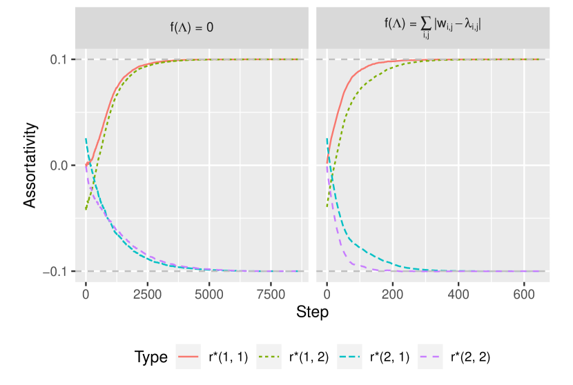
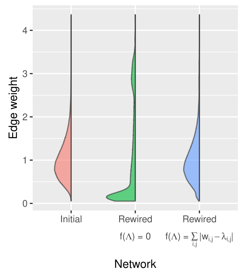
Figure 8: Average trace and edge weight density plots for PA networks with $m=1000$, $\alpha=\gamma=0.15$, $\beta=0.7$, and target assortativity coefficients $r^{*}(1,1)=r^{*}(1,2)=0.1$, $r^{*}(2,1)=r^{*}(2,2)=-0.1$. The left two panels are average trace plots based on objective functions $f(\bm{\Lambda})=0$ and $f(\bm{\Lambda})=\sum_{i,j}|w_{ij}-\lambda_{ij}|$. The right panel compares the density of edge weights of the initial networks and the constructed target networks under the same two objective functions.

The seed network for all of the extended PA networks in our simulation study contained one weighted edge $(1,2,1.0)$. The parameters were set to $\beta\in\{0.6,0.7,0.8\}$, $\alpha=\gamma=(1-\beta)/2$ and $\delta_{1}=\delta_{2}=1$. Again, $h$ was set to be a gamma distribution with shape $5$ and scale $0.2$. We considered PA networks of different sizes determined by number of evolutionary steps $m\in\{200,400,600,800,1000\}$. The number of replicates for each combination of $m$ and $\beta$ was $100$. The target assortativity coefficients for this series of simulation studies were also $r^{*}(1,1)=r^{*}(1,2)=0.1$ and $r^{*}(2,1)=r^{*}(2,2)=-0.1$.

The PA network simulation study yielded conclusions similar to those from the ER network simulation study, despite that the evolutionary processes of the two models are tremendously different. Since the results across different $m$ and $\beta$ combinations for PA networks are similar, we only report those for $m=1000$ and $\beta=0.7$ in Figure 8. The left two panels present the average trace plots obtained under different objective functions $f(\bm{\Lambda})=0$ and $f(\bm{\Lambda})=\sum_{i,j}|w_{ij}-\lambda_{ij}|$, where the reordering procedure was implemented to both. All the assortativity coefficients reach target values. More rewiring steps were needed for objective function $f(\bm{\Lambda})=0$, but less computing time was needed. Precisely, the median runtime was $43$ seconds with $f(\bm{\Lambda})=0$ and $142$ seconds for $f(\bm{\Lambda})=\sum_{i,j}|w_{ij}-\lambda_{ij}|$. The middle panel shows that more rewiring steps were required for $r^{*}(1,2)$ and $r^{*}(2,1)$. This was intuitively expected as their initial values were further away from the targets. The right panel shows again that the post-rewiring edge weight distribution using $f(\bm{\Lambda})=\sum_{i,j}|w_{ij}-\lambda_{ij}|$ is much closer than that using $f(\bm{\Lambda})=0$ to the edge weight distribution of the initial networks.

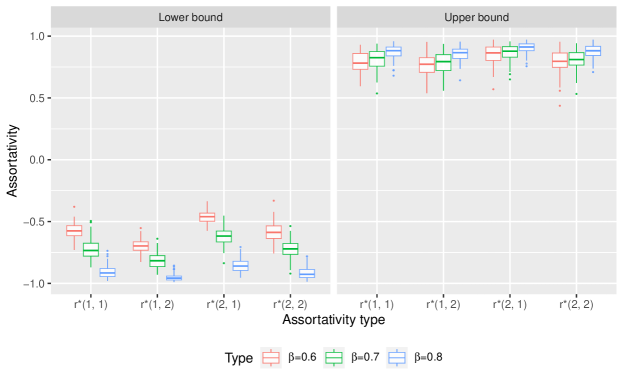
Figure 9: Side-by-side box plots of the upper and lower bounds of the assortativity coefficients of PA networks with $m=1000$, $\beta\in\{0.6,0.7,0.8\}$ and $\alpha=\gamma=(1-\beta)/2$.

Finally, the box plots of the lower and upper bounds of the attainable assortativity coefficients based on 100 replicates for the simulated PA networks with the number of evolutionary steps $m=1000$ are shown in Figure 9. With the same value of $m$, the number of edges was fixed, and a larger $\beta$ resulted in a denser network. The range of assortativity coefficients for large $\beta$ was found wider than that for small $\beta$, as larger $\beta$ caused greater variances for node in- and out-strengths.

5 Discussions

The SSRP algorithm tackles the rewiring problem of Newman (2003) towards predetermined assortativity levels in the context of weighted, directed networks. The rewiring retains the certain critical network properties such as the marginal node out- and in-strength distributions and the sparsity. The essential idea of the proposed approach is determining the adjacency matrix of a target network by solving a mixed integer programming problem, followed by a sweeping procedure to transform the initial network to the target by using rewiring. More complex objective functions could be used in setting up the mixed integer programming problem at extra computational costs to minimize the change in the edge weight distribution. The proposed algorithm is also applicable to unweighted or undirected networks with minor modifications.

There is a major difference between the SSRP algorithm and other rewiring methods like Newman’s algorithm (Newman, 2003) and the DiDPR algorithm (Wang et al., 2022). The SSPR algorithm derives an exact solution of target network with predetermined assortativity measures, but the others aim to find an approximated solution, that is, they search a target network with assortativity measures whose expectations equal to the given values. Accordingly, the determination of target networks differs between SSPR and other methods, too. SSRP directly works on adjacency matrix calculation, whereas the other methods determine target adjacency matrix through joint node-degree distributions governed by given assortativity measures. This difference means an advantage for the SSRP algorithm in some applications and a limitation in other applications. Extending the DiDPR algorithm in Newman’s sense to generating weighted, directed networks remains an open question, yet challenging for preserving network sparsity or other critical network properties in addition to marginal node degree or strength distributions.

Appendix A Proof of Proposition 3.1

Proof.

Without loss of generality, assume $\psi_{ij}>0$. Since we have $\sum_{j=1}^{n}\psi_{ij}=0$ according to the rewiring setup, there exists a nonempty set $S_{j}\subseteq\{j+1,j+2,\ldots,n\}$ such that $\psi_{ij^{\ast}}<0$ for all $j^{\ast}\in S_{j}$ and $\psi_{ij}+\sum_{j^{\ast}\in S_{j}}\psi_{ij^{\ast}}\leq 0$, where the equality holds if $\psi_{ij}$ is the only positive element in the $i$-th row. Similarly, due to $\sum_{i=1}^{n}\psi_{ij}=0$, for each $\psi_{ij^{\ast}}$ with $j^{\ast}\in S_{j}$, there exists $T_{i}\subseteq\{i+1,i+2,\ldots,n\}$ such that $\psi_{i^{\ast}j^{\ast}}>0$ for all $i^{\ast}\in T_{i}$ and $\psi_{ij^{\ast}}+\sum_{i^{\ast}\in T_{i}}\psi_{i^{\ast}j^{\ast}}\geq 0$.

It follows that

$$\sum_{j^{\ast}\in S_{j}}\sum_{i^{\ast}\in T_{i}}\psi_{i^{\ast}j^{\ast}}\geq\psi_{ij},$$

which suggests that, for each pair of $(i^{\ast},j^{\ast})$, there exists $0\leq u_{i^{\ast}j^{\ast}}\leq\psi_{i^{\ast}j^{\ast}}$ giving rise to

$$\sum_{j^{\ast}\in S_{j}}\sum_{i^{\ast}\in T_{i}}u_{i^{\ast}j^{\ast}}=\psi_{ij}.$$

Therefore, there exists a path continuously rewiring $(v_{i},v_{j},w_{ij})$ and $(v_{i^{\ast}},v_{j^{\ast}},w_{i^{\ast}j^{\ast}})$ with $\Delta w=u_{i^{\ast}j^{\ast}}$ for all $i^{\ast}$ and $j^{\ast}$ leading to $\psi_{ij}=0$.

The proof for $\psi_{ij}<0$ can be done mutatis mutandis. ∎

References

- Barabási (2016) Barabási, A.-L. (2016). Network Science. Cambridge, UK: Cambridge University Press.
- Barabási and Albert (1999) Barabási, A.-L. and R. Albert (1999). Emergence of scaling in random networks. Science 286(5439), 509–512.
- Chan and Akoglu (2016) Chan, H. and L. Akoglu (2016). Optimizing network robustness by edge rewiring: A general framework. Data Mining and Knowledge Discovery 30(5), 1395–1425.
- Erdös and Rényi (1959) Erdös, P. and A. Rényi (1959). On random graphs I. Publicationes Mathematicae Debrecen 6, 290–297.
- Gilbert (1959) Gilbert, E. N. (1959). Random graphs. Annals of Mathematical Statistics 30(4), 1141–1144.
- Gurobi Optimization, LLC (2023) Gurobi Optimization, LLC (2023). gurobipy: Python Interface to Gurobi. Version 10.0.1.
- IBM (2022) IBM (2022). User’s Manual for CPLEX.
- Iorio et al. (2016) Iorio, F., M. Bernardo-Faura, A. Gobbi, T. Cokelaer, G. Jurman, and J. Saez-Rodriguez (2016). Efficient randomization of biological networks while preserving functional characterization of individual nodes. BMC Bioinformatics 17, 542.
- Newman (2003) Newman, M. E. J. (2003). Mixing patterns in networks. Physical Review E 67(2), 026126.
- Schweimer et al. (2022) Schweimer, C., C. Gfrerer, F. Lugstein, D. Pape, J. A. Velimsky, R. Elsässer, and B. C. Geiger (2022). Generating simple directed social network graphs for information spreading. In F. Laforest, T. R., E. Simperl, A. D., A. Gionis, I. Herman, and L. Médini (Eds.), Proceedings of the ACM Web Conference 2022 (WWW ’22), New York, NY, USA, pp. 1475–1485. Association for Computing Machinery.
- Staples et al. (2015) Staples, P. C., E. L. Ogburn, and J.-P. Onnela (2015). Incorporating contact network structure in cluster randomized trials. Scientific Reports 5, 17581.
- Uribe-Leon et al. (2020) Uribe-Leon, C., J. C. Vasquez, M. A. Giraldo, and G. Ricaurte (2020). Finding optimal assortativity configurations in directed networks. Journal of Complex Networks 8(6), cnab004.
- Van Mieghem et al. (2010) Van Mieghem, P., H. Wang, X. Ge, S. Tang, and F. A. Kuipers (2010). Influence of assortativity and degree-preserving rewiring on the spectra of networks. The European Physical Journal B 76, 643–652.
- Wan et al. (2017) Wan, P., T. Wang, R. A. Davis, and S. I. Resnick (2017). Fitting the linear preferential attachment model. Electronic Journal of Statistics 11, 3738–3780.
- Wang et al. (2022) Wang, T., J. Yan, Y. Yuan, and P. Zhang (2022). Generating directed networks with predetermined assortativity measures. Statistics and Computing 32(5), 91.
- Wuellner et al. (2010) Wuellner, D. R., S. Roy, and R. M. D’Souza (2010). Resilience and rewiring of the passenger airline networks in the United States. Physical Review E 82(5), 056101.
- Yuan et al. (2023) Yuan, Y., T. Wang, J. Yan, and P. Zhang (2023). Generating general preferential attachment networks with R package wdnet. Journal of Data Science 21(3), 538–556.
- Yuan et al. (2021) Yuan, Y., J. Yan, and P. Zhang (2021). Assortativity measures for weighted and directed networks. Journal of Complex Networks 9(2), cnab017.