A robust Bayesian meta-analysis for Estimating the Hubble Constant via Time Delay Cosmography

Abstract

We propose a Bayesian meta-analysis to infer the current expansion rate of the Universe, called the Hubble constant ($H_{0}$), via time delay cosmography. Inputs of the meta-analysis are estimates of two properties for each pair of gravitationally lensed images; time delay and Fermat potential difference estimates with their standard errors. A meta-analysis can be appealing in practice because obtaining each estimate from even a single lens system involves substantial human efforts, and thus estimates are often separately obtained and published. This work focuses on combining these estimates from independent studies to infer $H_{0}$ in a robust manner. For this purpose, we adopt Student’s $t$ error for the inputs of the meta-analysis. We investigate properties of the resulting $H_{0}$ estimate via two simulation studies with realistic imaging data. It turns out that the meta-analysis can infer $H_{0}$ with sub-percent bias and about 1% level of coefficient of variation, even when 30% of inputs are manipulated to be outliers. We also apply the meta-analysis to three gravitationally lensed systems, and estimate $H_{0}$ by $75.632\pm 6.918$ (km/second/Mpc), which covers a wide range of $H_{0}$ estimates obtained under different physical processes. An R package h0 is publicly available for fitting the proposed meta-analysis.

and

1 Introduction

Estimates of the Hubble constant $H_{0}$ under the standard cosmological model, that is, the flat $\Lambda$ Cold Dark Matter ($\Lambda$CDM) model, have been inconsistent, causing a tension between measurements of $H_{0}$ from early and late Universe (Verde, Treu and Riess, 2019; Di Valentino et al., 2021; Shah, Lemos and Lahav, 2021; Abdalla et al., 2022). For example, the most recent probe on the early Universe infers $H_{0}$ by $67.4\pm 0.5$ km s^-1 Mpc^-1 via the cosmic microwave background experiment (Planck Collaboration et al., 2020). The unit of the Hubble constant is kilometer/second/megaparsec, typically denoted by km s^-1 Mpc^-1. It means that if we were 1 megaparsec (that is about 3.26 million light years) away from the Earth, then objects would move away by 1 kilometer per second due to the expansion of the Universe. We omit the unit of $H_{0}$ hereafter. On the other hand, the most recent $H_{0}$ estimate based on a locally calibrated comic distance ladder (that is, from the late Universe) is $73.04\pm 1.04$ (Riess et al., 2022), which is claimed to be 5 standard deviations away from the early Universe study. These inconsistent estimates between the early and late Universe measurements have raised a question about the validity of the underlying standard cosmological model and brought up a possibility of new physics. To check whether the tension is due to unknown systematic error of measurements, astronomers have improved data quality and inferential accuracy of existing methods, for example, Riess et al. (2019), Riess et al. (2021), and Riess et al. (2022). Various methods have also been developed under different physical processes to better understand the systematic error and test the standard cosmological model.

As a completely independent way to infer the Hubble constant, time delay cosmography adopts strong gravitational lensing effects of quasars (Refsdal, 1964; Linder, 2011; Treu and Marshall, 2016; Suyu et al., 2017; Birrer et al., 2022; Treu, Suyu and Marshall, 2022). When a galaxy is geometrically aligned between a quasar and the Earth, the strong gravitational field of the intervening galaxy bends the trajectories of light photons emitted from the quasar, as illustrated in the left panel of Figure 1. The deflected light rays travel toward the Earth. As a result we see multiple (mostly two or four) images of the same quasar in the sky. The right panel of Figure 1 shows an image of a doubly-lensed strong lens system, simulated by a Python package lenstronomy (Birrer and Amara, 2018; Birrer et al., 2021), as an example of what we expect to see in the sky via a telescope. The faint image at the center is the intervening lensing galaxy, and the two bright images located to the south and north from the center are the two lensed images of the same quasar. We call it a strong gravitational lensing effect (Schneider, Wambsganss and Kochanek, 2006; Treu, 2010). The travel times of light photons for each lensed image can be different depending on the paths they take because the length of each path may differ and photons may pass through different gravitational potential of the intervening galaxy. We call such differences between their travel times time delays.

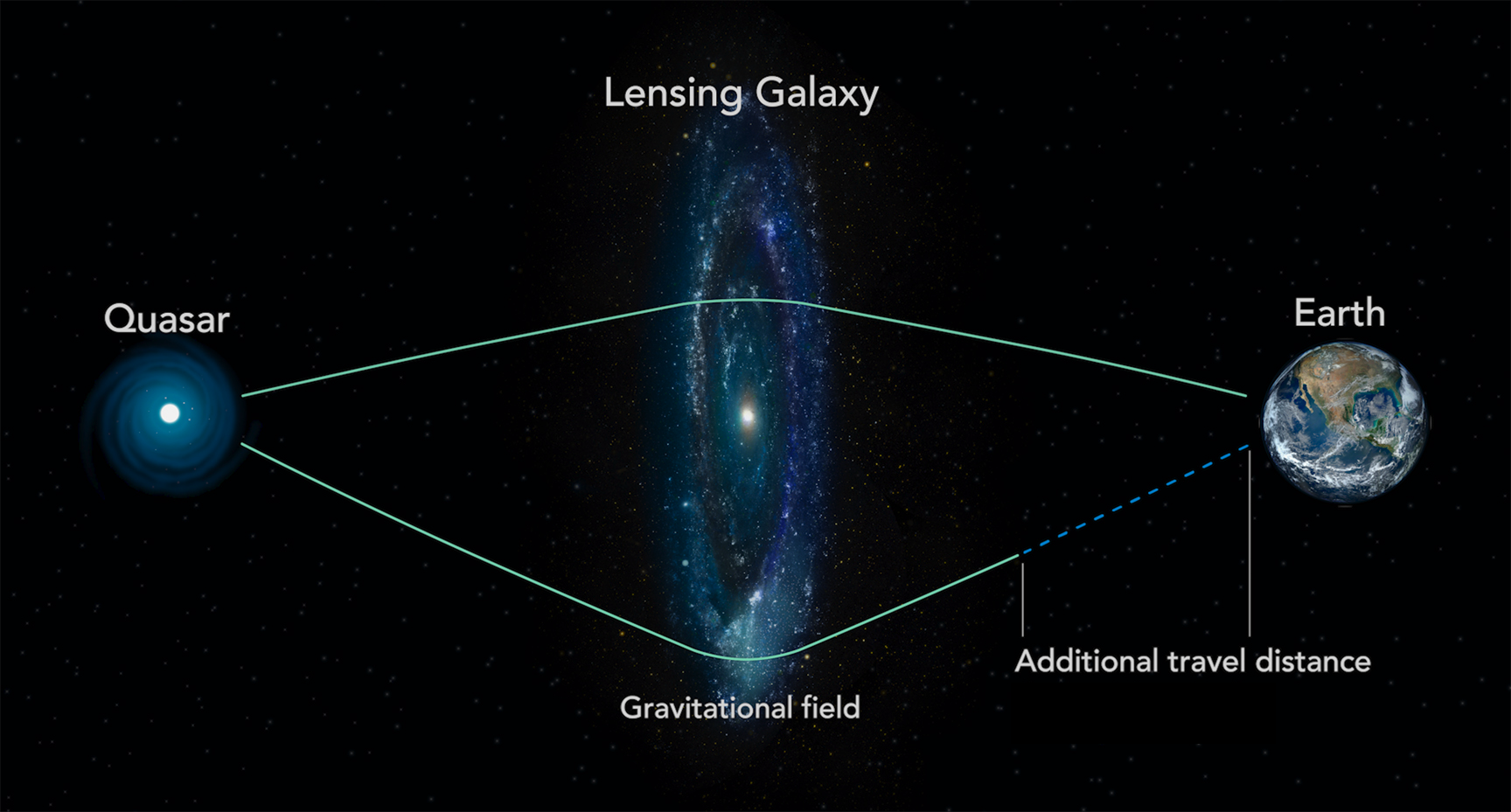
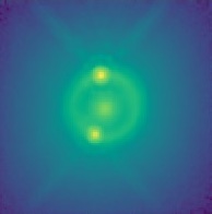
Figure 1: Strong gravitational lensing is illustrated in the left panel. When a galaxy is intervening between a quasar and the Earth, light photons emitted by the quasar take different routes to the Earth because the strong gravitational field of the intervening galaxy bends the trajectories of photons (Image Credit: Michael Fleck). In this case we see multiple images of the same quasar in the sky. The right panel shows simulated imaging data of a doubly-lensed system obtained by a Python package lenstronomy (Birrer and Amara, 2018; Birrer et al., 2021); the faint image at the center is the intervening lensing galaxy and the two brightest images around the center are the two lensed images of the same quasar.

For each pair of lensed images (one pair for a doubly-lensed system, and at least three pairs for a quadruply-lensed system), time delay cosmography models the additional travel distance of the longer route by a physical equation that interweaves cosmological parameters and measurable quantities. Two of the measurable quantities are time delay and Fermat potential difference, and these can be separately estimated from two different types of data. Time delay estimates are obtained from several time series data of brightness of multiply-lensed quasar images (Tewes et al., 2013; Eulaers et al., 2013; Liao et al., 2015; Tak et al., 2017; Courbin et al., 2018; Bonvin et al., 2016, 2018, 2019; Millon et al., 2020a; Meyer et al., 2023). On the other hand, Fermat potential differences are estimated from high-resolution imaging data of each lens system, such as the one in the right panel of Figure 1 (Birrer and Amara, 2018; Rusu et al., 2020; Wong et al., 2020; Birrer et al., 2020; Shajib et al., 2020; Ding et al., 2021a, b; Shajib et al., 2022; Ertl et al., 2023; Schmidt et al., 2023).

These two types of data are independently obtained, and thus the inferences on time delays and differences in Fermat potential can be performed separately without knowing each other. This aspect has enabled astronomers to conduct a so-called blind analysis to estimate each component independently and combine these to infer $H_{0}$ in the end (Suyu et al., 2013, 2017). Also, it is well known that estimating time delays and Fermat potential differences from even a single lens system requires substantial human efforts. For instance, each estimation procedure goes through data pre-processing, visual inspection for identifying anomalies, modeling the data with physical processes, model fitting and checking, and interpretation (Shajib et al., 2019; Leon-Anaya et al., 2023). Details of each step may be different according to the types of the data (time series or imaging data). Consequently, these estimates are often published separately in the literature. For instance, time delay estimates (Millon et al., 2020a) and Fermat potential difference estimates (Ertl et al., 2023; Schmidt et al., 2023) of a strong lens system 2M1134–2103 are independently estimated and separately published.

We focus on how to combine these estimates available in the literature to estimate $H_{0}$ via a meta-analysis (Gelman et al., 2013, Chapter 5.6). The meta-analysis is built on the estimates of time delays and those of Fermat potential differences, instead of modeling time series data and high-resolution imaging data from scratch. We adopt a Student’s $t_{4}$ measurement error model by assuming that the input estimates are measured around unknown true values with scaled Student’s $t_{4}$ noises. The scale is set to the given standard error of the estimate, and thus it is assumed to be fully known. This heavy-tailed error assumption makes the model robust to potential outliers. Next, we incorporate physical equations into the model to interweave the unknown true values, additionally accounting for more source of uncertainty such as an effect of the mass along the line of sight between the lens and the observer. The model ends up with $(2+K)$ parameters, where $K$ is the number of lens systems in the data. Weakly informative Uniform and Cauchy priors are assumed on these $(2+K)$ model parameters. An R package h0 fits the model via Metropolis-Hastings within Gibbs sampling (Metropolis et al., 1953; Geman and Geman, 1984; Tierney, 1994). It takes about 2,900 seconds on average to draw 10,000 posterior samples when the data are composed of 90 input pairs (time delay and Fermat potential difference) of 30 quadruply-lensed systems.

Our numerical studies based on both simulated and realistic data show that the proposed meta-analysis can produce an accurate $H_{0}$ estimate even in the presence of outlying inputs. The first numerical study is based on a simulated data set publicly available from the Time Delay Lens Modeling Challenge (Ding et al., 2021a), a blind data analytic competition held from 2018 to 2019. Specifically, we check how the $H_{0}$ estimate changes when we manipulate more and more input data to be wrong or outliers. It shows that the $H_{0}$ estimate is robust even when 30% of the 40 inputs from 16 lens systems are modified to be outliers. The second numerical study is based on realistic data of 90 input pairs from 30 quad-lens systems analyzed by the STRIDE science collaboration (Schmidt et al., 2023). This simulation also confirms that the meta-analysis can recover their underlying cosmological parameters in a robust manner when 30% of data are manipulated to be outliers. Finally, we apply the meta-analysis to three strong lens systems, and estimate $H_{0}$ by $75.632\pm 6.918$. This estimate is consistent to previous $H_{0}$ estimates under time delay cosmography, for example, 73.3${}^{+1.7}_{-1.8}$ in Wong et al. (2020), 74.2 ${}^{+2.7}_{-3.0}$ in Shajib et al. (2020), and 74.5 ${}^{+5.6}_{-6.1}$ in Birrer et al. (2020), not to mention the estimates from the early and late Universe measurements in tension.

The rest of this article is organized as follows. We describe details of time delay cosmography in Section 2 and outlines the proposed meta-analysis in Section 3. Modeling assumptions and model fitting procedures via maximum likelihood estimation and Bayesian posterior sampling appear in Section 4. We investigate the performance of the meta-analysis in two simulation settings in Sections 5.1 and 5.2, and explain how we obtain the $H_{0}$ estimate from the three lens systems in Section 6. We discuss limitations and future direction of the meta analysis in Section 7.

2 Overview of Time Delay Cosmography

Time delay cosmography infers $H_{0}$ using the information about the additional travel distance of the light caused by strong gravitational lensing, as visualized in the left panel of Figure 1. The following physical equation plays a key role in describing this additional travel distance (Refsdal, 1964):

$$c\Delta_{ijk}=D_{\Delta}(H_{0},z_{k},\Omega)\phi_{ijk},$$ (1)

where $c$ denotes the speed of light that is about $2.59\times 10^{10}$ kilometers per day, and $\Delta_{ijk}$ is the time delay in days between lensed images $i$ and $j$ of quasar $k$ ($k=1,2,\ldots,K$). Intuitively, the multiplication of these two quantities, $c\Delta_{ijk}$, on the left-hand side of Eqn (1) represents the additional travel distance caused by strong gravitational lensing in that the light speed (km/day) is multiplied by the additional travel time (day).

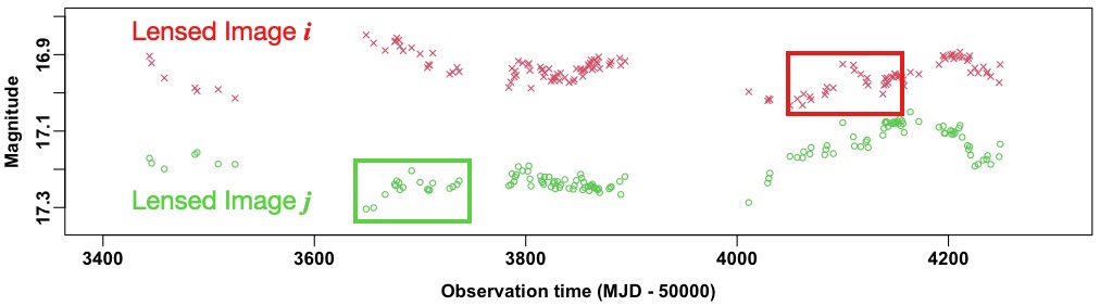
Figure 2: Time series data of brightness obtained by measuring brightness of doubly-lensed images of quasar Q0957+561 in $g$-band over time (Shalyapin, Goicoechea and Gil-Merino, 2012). Magnitude is an astronomical measure of brightness, observation time is in days, and MJD represents modified Julian day. A time delay estimate between two lensed images can be obtained by identifying a time lag between similar fluctuation patterns appearing in both time series.

Time delays are estimated from multiple time series data of brightness of lensed images. These data are obtained by measuring brightness of multiply lensed images of the same source in the sky, such as the two bright images around the center in the right panel of Figure 1. For instance, Figure 2 exhibits two time series data of brightness (magnitude) for doubly lensed images ($i$ and $j$) of quasar Q0957+561, observed in $g$-band (Shalyapin, Goicoechea and Gil-Merino, 2012). Here, it is not difficult to identify similar fluctuation patterns appearing in both time series, such as those appearing in two rectangles, with about 400-day-long time lag. A model-based approach to time delay estimation treats this time lag as an unknown parameter to be estimated. For example, Hu and Tak (2020) estimate the time delay of this data set as 413.392 days by adopting a damped random walk model (Kelly, Bechtold and Siemiginowska, 2009) to describe stochastic variability of the time series data.

The right-hand side of Eqn (1) re-expresses the additional travel distance under the Einstein’s general relativity, accounting for light photons traveling in the curved space and time caused by the strong gravitational field of the intervening galaxy. The notation $z_{k}=\{z_{sk},z_{dk}\}$ indicates a vector for two redshifts measuring how fast the $k$-th quasar ($z_{sk}$) and lensing galaxy ($z_{dk}$) are moving away from the observer; the subscripts $s$ and $d$ denote ‘source (quasar)’ and ‘deflector (lens)’, respectively. These redshifts can be accurately measured via spectroscopic data, and thus we assume that the vector $z_{k}$ is fully known for all $k$. The next notation $\Omega=\{\Omega_{\textrm{m}},\Omega_{\Lambda}\}$ represents a vector for two cosmological parameters, the present-day dark matter density $\Omega_{\textrm{m}}$ and dark energy density $\Omega_{\Lambda}$. Since their sum is one under the standard cosmological model, that is, $\Omega_{\textrm{m}}+\Omega_{\Lambda}=1$, we consider $\Omega_{\textrm{m}}$ as the only unknown parameter in $\Omega$. Hereafter, we use $\Omega$ or $\Omega_{\textrm{m}}$ exchangeably.

The notation $D_{\Delta}(H_{0},z_{k},\Omega)$ denotes the time delay distance in the unit of megaparsec (Mpc) defined as a ratio of three angular diameter distances from the observer to the deflector ($D_{d}$), from the observer to the source ($D_{s}$), and from the deflector to the source ($D_{ds}$). Figure 3 visualizes these angular diameter distances. Specifically, these three distances are deterministic functions of $H_{0},z_{k}$, and $\Omega$:

$$\begin{aligned} D_{d}(H_{0},z_{k},\Omega)&=\frac{c\int_{0}^{z_{dk}}\frac{du}{W(u;\Omega)}}{(1+z_{dk})H_{0}},~{}~{}~{}~{}~{}D_{s}(H_{0},z_{k},\Omega)=\frac{c\int_{0}^{z_{sk}}\frac{du}{W(u;\Omega)}}{(1+z_{sk})H_{0}},~{}\textrm{and}\\ D_{ds}(H_{0},z_{k},\Omega)&=\frac{c}{(1+z_{sk})H_{0}}\left(\int_{0}^{z_{sk}}\frac{du}{W(u;\Omega)}-\int_{0}^{z_{dk}}\frac{du}{W(u;\Omega)}\right)\end{aligned}$$ (2)

The notation $W(u;\Omega)$ denotes a deterministic function of $u$ given the cosmological parameters, $\Omega_{\textrm{m}}$ and $\Omega_{\Lambda}$. Specifically, $W(u;\Omega)=((1+u)^{3}\Omega_{\textrm{m}}+\Omega_{\Lambda})^{0.5}$ under the standard cosmological model; see Hogg (1999) for details of cosmological distance measures. Then the time delay distance of lens system $k$ is defined by these angular diameter distances:

$$\begin{aligned} D_{\Delta}(H_{0},z_{k},\Omega)&=(1+z_{dk})\frac{D_{d}(H_{0},z_{k},\Omega)D_{s}(H_{0},z_{k},\Omega)}{D_{ds}(H_{0},z_{k},\Omega)}\\ &{\color[rgb]{0,0,0}=\frac{c\left(\int_{0}^{z_{dk}}\frac{du}{W(u;\Omega)}\right)\left(\int_{0}^{z_{sk}}\frac{du}{W(u;\Omega)}\right)}{H_{0}\left(\int_{0}^{z_{sk}}\frac{du}{W(u;\Omega)}-\int_{0}^{z_{dk}}\frac{du}{W(u;\Omega)}\right)}}.\end{aligned}$$ (3)

Clearly, the time delay distance $D_{\Delta}(H_{0},z_{k},\Omega)$ is inversely proportional to $H_{0}$, making it useful for the Hubble constant estimation (Suyu et al., 2017; Treu, Suyu and Marshall, 2022).

The last quantity $\phi_{ijk}$ in Eqn (1) is the difference in Fermat potential that light rays of lensed images $i$ and $j$ of the $k$-th lens system pass through (Schneider, Wambsganss and Kochanek, 2006, Section 2.2). This represents the different extents to the light deflection and to scaled gravitational potential at two different regions of the gravitational field. Specifically this Fermat potential difference is defined as

$$\phi_{ijk}=\phi(\theta_{ik},\theta_{jk},\beta_{k})=\frac{1}{2}(\theta_{ik}-\beta_{k})^{2}-\psi(\theta_{ik})-\left(\frac{1}{2}(\theta_{jk}-\beta_{k})^{2}-\psi(\theta_{jk})\right).$$ (4)

Here $\theta_{ik}$ and $\theta_{jk}$ are the apparent angular positions of lensed images $i$ and $j$ of source $k$ on the sky, respectively, and each is a vector of length two for angular coordinates (ascension and declination). The notation $\beta_{k}$ is the apparent angular position of source $k$ that could have been observed without a lens. In practice, we cannot observe $\beta_{k}$ because the intervening lensing galaxy blocks the line of sight between the source and the observer. The difference between $\theta_{ik}$ and $\beta_{k}$ in Eqn (4) is called the scaled deflection angle of the lensed image $i$ of source $k$, which is typically denoted by $\alpha(\theta_{ik})$ in the literature. This relationship forms a so-called lens equation, $\beta_{k}=\theta_{ik}-\alpha(\theta_{ik})$ for any lensed image $i$. These angular positions and deflection angle are illustrated in Figure 3 with one lensed image. Lastly, $\psi(\theta_{ik})$ and $\psi(\theta_{jk})$ are scaled gravitational potential of the lensing galaxy (or simply called lens potential) at the positions of lensed images, $\theta_{ik}$ and $\theta_{jk}$, respectively. The lens potential function must satisfy two conditions. First, the gradient of each lens potential becomes the scaled deflection angle, that is, $\alpha(\theta_{ik})=\nabla\psi(\theta_{ik})$, so that the gradient of Fermat potential is zero according to the Fermat’s principle. Second, one half of the Laplacian becomes the dimensionless surface mass density $\kappa(\theta_{ik})~{}(=\nabla^{2}\psi(\theta_{ik})/2$). This dimensionless density can also be expressed as $\kappa(\theta_{ik})=\Sigma(\theta_{ik})/\Sigma_{\textrm{cr}}$, where $\Sigma(\theta_{ik})$ is the surface mass density function and $\Sigma_{\textrm{cr}}$ is the critical mass density.

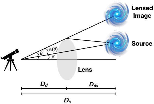
Figure 3: Angular distances and positions. Angular diameter distance from the observer to the deflector (lens) is $D_{d}$, that from the observer to the source is $D_{s}$, and that from the deflector to the source is $D_{ds}$. Angular position of the lensed image is $\theta$, and that of the source is $\beta$. The scaled deflection angle of the lensed image at $\theta$ is denoted by $\alpha(\theta)$, satisfying the lens equation $\beta=\theta-\alpha(\theta)$.

Thus, the lens modeling starts by adopting a functional form of this surface mass density, $\Sigma(\theta_{ik})$; its integral becomes $\alpha(\theta_{ik})$ and its double-integral is the lens potential $\psi(\theta_{ik})$. Stellar kinematic information can be incorporated into the model to handle mass-sheet degeneracy, an effect that different lens mass model can produce the same observations (Gorenstein, Falco and Shapiro, 1988; Birrer, Amara and Refregier, 2016; Yıldırım et al., 2021; Shajib et al., 2023). In addition to this lens mass model, surface brightness is also modeled for each of lens and source. With a set of unknown parameters in these lens mass, lens light, and surface light models, including unknown angular positions, one can simulate imaging data, that is, a model prediction of the imaging data given the model parameters. Then, a likelihood function of all of the model parameters can be obtained by an independent Gaussian assumption on the observed light intensity in each pixel whose mean is the pixel-wise model prediction of light intensity. See Section 5 of Birrer et al. (2022) for more details of this estimation procedure.

Besides the explicitly stated quantities in Eqn (1), astronomers account for the effect of the mass structure along the line of sight between the lens and the observer because it is known to be an important source of bias and extra uncertainty in $H_{0}$ estimation (Suyu et al., 2010; Schneider and Sluse, 2013; Suyu et al., 2013, 2014; Sereno and Paraficz, 2014; Rusu et al., 2017; Buckley-Geer et al., 2020; Tihhonova et al., 2020; Fleury, Larena and Uzan, 2021; Wells, Fassnacht and Rusu, 2023; Treu, Suyu and Marshall, 2022, Section 3.2.4). This effect is characterized by a quantity called external convergence, denoted by $\kappa_{\text{ext},k}$ for each lens system $k$, whose value is negative if the line of sight has less dense structure than the overall density of the Universe and is positive for more dense structure. The time delay distance after accounting for this line-of-sight effect is defined as

$$D_{\Delta}^{\textrm{ext}}(H_{0},z_{k},\Omega)=\frac{D_{\Delta}(H_{0},z_{k},\Omega)}{1-\kappa_{\text{ext},k}}.$$ (5)

Since the Hubble constant is inversely proportional to the time delay distance, this line-of-sight effect is propagated to the Hubble constant as follows.

$$H_{0}^{\textrm{ext}}=(1-\kappa_{\textrm{ext},k})H_{0}.$$ (6)

Because of this relationship, a positive value of $\kappa_{\textrm{ext},k}$ means that $H_{0}$ will be over-estimated if we do not account for the over-dense line-of-sight effect. Also, the uncertainty of the resulting $H_{0}^{\textrm{ext}}$ estimate will also be affected by the multiplication factor $(1-\kappa_{\textrm{ext},k})$. This quantity $\kappa_{\textrm{ext},k}$ can be estimated from external data by comparing the number of galaxies in the lens field of interest with the counts of galaxies in similar reference fields, without knowing the time delay and Fermat potential difference estimates. See Wells, Fassnacht and Rusu (2023) for more details of modeling the external convergence.

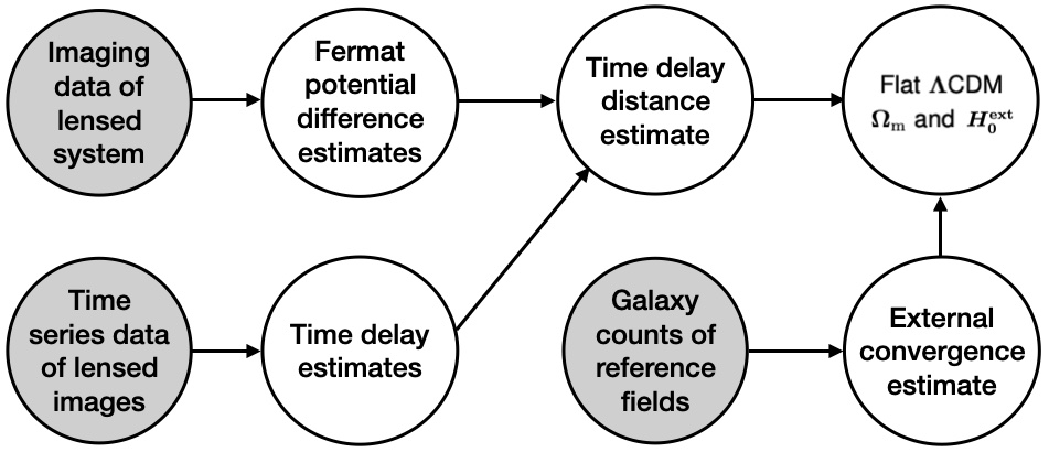
Figure 4: This diagram illustrates a series of estimation steps towards the Hubble constant $H_{0}^{\text{ext}}$. The gray circles indicate the observed data.

3 Meta-Analysis

Time delay cosmography is a comprehensive framework to infer $H_{0}$ based mainly on physical equation in Eqn (1). The equation relates six quantities, that is, light speed $c$, time delay $\Delta_{ijk}$, the Hubble constant $H_{0}$, redshifts $z_{k}$, cosmological parameter $\Omega$, and Fermat potential difference $\phi_{ijk}$. Among these, two quantities, $c$ and $z_{k}$ are fixed at known constants. The time delays ($\Delta_{ijk}$’s) and Fermat potential differences ($\phi_{ijk}$’s) are independently estimated from multiple time series data of brightness of lensed images and from high-resolution imaging data, respectively. These estimates can constrain the time delay distance $D_{\Delta}(H_{0},z_{k},\Omega)$ via Eqn (1) for all $k$, and then the information about these multiple time delay distances, $D_{\Delta}(H_{0},z_{1},\Omega)$, $D_{\Delta}(H_{0},z_{2},\Omega)$, $\ldots$, $D_{\Delta}(H_{0},z_{K},\Omega)$ can constrain $H_{0}$ and $\Omega$ in turn. To account for potential bias and extra uncertainty caused by the line-of-sight effect, astronomers incorporate external convergence into the model and finally estimate $H_{0}^{\text{ext}}$. Figure 4 illustrates this series of inferential steps toward $H_{0}^{\text{ext}}$ under time delay cosmography in a simplified manner. The circles in gray indicate the observed data.

Estimating $H_{0}$ via time delay cosmography requires enormous efforts of more than a hundred experts from various fields of astronomy. For example, there are 82 experts in Treu et al. (2018) for newly identifying seven strong lens candidates, 71 in Schmidt et al. (2023) for estimating Fermat potential differences of 30 lens systems, 68 in Buckley-Geer et al. (2020) for estimating line-of-sight effects of two lens systems, and 28 in Millon et al. (2020a) for estimating time delays of six lens systems. Also, there are at least five scientific collaboration groups contributing to time delay cosmography; COSMOGRAIL collaboration (Eigenbrod et al., 2005); H0LiCOW collaboration (Suyu et al., 2017); STRIDES collaboration (Treu et al., 2018); SHARP collaboration (Chen et al., 2019); and TDCOSMO collaboration (Millon et al., 2020b). These are clear evidence that the Hubble constant estimation via time delay cosmography is not only of great interest in astronomy, but also challenging enough to require enormous human efforts and time.

Our motivation is that a meta-analysis can save such humongous efforts by extracting the information about $H_{0}$ from various estimates separately published in the literature, as the information is commonly embedded in these independent studies. Moreover, since there are not many strong lens systems suitable for accurate $H_{0}$ estimation, for example, with six to eight lens systems (Shajib et al., 2020; Wong et al., 2020; Birrer et al., 2020; Denzel et al., 2021; Wang et al., 2022), it is crucial to prevent outlying inputs from unduly influencing the $H_{0}$ estimation.

Thus, we propose a robust meta-analysis based on Student’s $t$ error that takes the time delay and Fermat potential difference estimates as inputs, without modeling the time series and imaging data from scratch. We incorporate the external convergence of each lens system into the model as unknown model parameters, instead of estimating them from external data. Unlike the common practice in time delay cosmography, the meta-analysis does not separately estimate time delay distances, $D_{\Delta}(H_{0},z_{k},\Omega)$’s, before constraining $H_{0}$ and $\Omega$. Instead, it treats these deterministic functions as a medium to access the information about $H_{0}$ and $\Omega$ from the inputs. This has an effect of increasing the data size. For example, a quad-lens system $k$ produces at least three pairs of Fermat potential difference and time delay estimates, such as $(\hat{\phi}_{12k},\hat{\Delta}_{12k})$, $(\hat{\phi}_{13k},\hat{\Delta}_{13k})$, and $(\hat{\phi}_{14k},\hat{\Delta}_{14k})$. The meta-analysis treats these as three independent inputs that contain the information about $H_{0}$, instead of reducing these three pairs to one time delay distance estimate, $\hat{D}_{\Delta}(H_{0},z_{k},\Omega)$, to infer $H_{0}$. Treating the three paired estimates as three independent observations does not mean that each pair equally contributes to the $H_{0}$ estimate because each pair of estimates has different uncertainty levels (standard errors). Figure 5 illustrates a workflow of the meta-analysis.

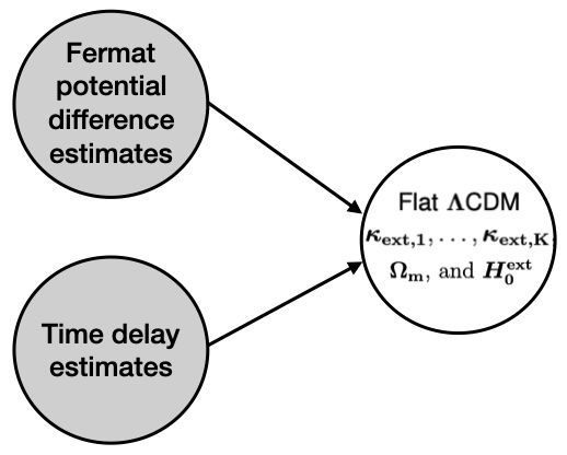
Figure 5: This diagram illustrates how the meta-analysis infers the Hubble constant $H_{0}$. The gray circles indicate the input data that are pairs of the Fermat potential difference and time delay estimates. The meta-analysis treats time delay distance $D_{\Delta}(H_{0},z_{k},\Omega)$ for each lens system $k$ as a deterministic function of $H_{0}$, $z_{k}$, and $\Omega$, as its notation indicates, instead of treating each time delay distance as a quantity to be estimated before constraining $H_{0}$ and $\Omega$. Also, the meta-analysis accounts for the line-of-sight effect by treating external convergences, $\kappa_{\text{ext},1},\ldots,\kappa_{\text{ext},K}$, as unknown model parameters.

4 Statistical Modeling and Inference

We derive the likelihood function of $H_{0}$, $\Omega$, and $\kappa_{\text{ext},k}$’s by combining Eqns (1) and (5), assuming that the time delay and Fermat potential difference constrain $D^{\text{ext}}_{\Delta}(H_{0},z_{k},\Omega)$, instead of $D_{\Delta}(H_{0},z_{k},\Omega)$ in Eqn (1). That is,

$$c\Delta_{ijk}=D_{\Delta}^{{\color[rgb]{0,0,0}\text{ext}}}(H_{0},z_{k},\Omega)\phi_{ijk}=\frac{D_{\Delta}(H_{0},z_{k},\Omega)\phi_{ijk}}{{\color[rgb]{0,0,0}1-\kappa_{\text{ext},k}}}.$$ (7)

Then, the Fermat potential difference can be expressed as

$$\phi_{ijk}={\color[rgb]{0,0,0}\frac{(1-\kappa_{\text{ext},k})c\Delta_{ijk}}{D_{\Delta}(H_{0},z_{k},\Omega)}}.$$ (8)

Applying a Gaussian assumption on the Fermat potential difference estimate, as proposed in an unpublished work of Marshal et al., we obtain the following Gaussian distribution of the Fermat potential difference estimate centered at the unknown true Fermat potential difference $\phi_{ijk}$ in Eqn (8):

$$\hat{\phi}_{ijk}\mid H_{0},\Omega,\Delta_{ijk},{\color[rgb]{0,0,0}\alpha_{ijk},\kappa_{\text{ext},k}}\sim N\!\left(\frac{{\color[rgb]{0,0,0}(1-\kappa_{\text{ext},k})}c\Delta_{ijk}}{D_{\Delta}(H_{0},z_{k},\Omega)},~{}~{}{\color[rgb]{0,0,0}\alpha_{ijk}}\hat{\sigma}^{2}_{\phi_{ijk}}\right),$$ (9)

where $\hat{\sigma}_{\phi_{ijk}}$ is the given standard error of $\hat{\phi}_{ijk}$, and $\alpha_{ijk}$ is an unknown variance adjustment factor to account for extra uncertainty beyond the given standard error, which is called an error-on-the-error approach in particle physics (Cowan, 2019). This adjustment factor later transforms Gaussian measurement error into Student’s $t$ measurement error (Tak, Ellis and Ghosh, 2019). Conditioning on $(H_{0},\Omega,\Delta_{ijk},\kappa_{\text{ext},k})$ in Eqn (9) is equivalent to conditioning on $\phi_{ijk}$ because of their deterministic relationship in Eqn (8). Marshal et al. fix $\Omega_{\textrm{m}}~{}{\color[rgb]{0,0,0}(=\Omega~{}\text{in this work})}$ at 0.3, but we treat it as an unknown parameter to be estimated.

Similarly, we assume that the time delay estimate $\hat{\Delta}_{ijk}$ follows a Gaussian distribution (Birrer, Amara and Refregier, 2016, Section 4.6), whose mean is the unknown true time delay $\Delta_{ijk}$ and variance is equal to squared standard error , $\hat{\sigma}^{2}_{\Delta_{ijk}}$, multiplied by the same adjustment factor, $\alpha_{ijk}$:

$$\hat{\Delta}_{ijk}\mid\Delta_{ijk},{\color[rgb]{0,0,0}\alpha_{ijk}}\sim N\!\left({\Delta}_{ijk},~{}~{}{\color[rgb]{0,0,0}\alpha_{ijk}}\hat{\sigma}^{2}_{\Delta_{ijk}}\right).$$ (10)

Denoting all time delays by $\Delta=\{\Delta_{ijk}:i<j~{}\textrm{and}~{}k=1,2,\ldots,K\}$, all adjustment factors by $\alpha=\{\alpha_{ijk}:i<j~{}\textrm{and}~{}k=1,2,\ldots,K\}$, and all external convergences by $\kappa_{\text{ext}}=\{\kappa_{\text{ext},k}:k=1,2,\ldots,K\}$, we express the likelihood function of $H_{0},\Omega$, $\Delta$, $\alpha$, and $\kappa_{\text{ext}}$ as a multiplication of joint density functions of input data pairs, ($\hat{\phi}_{ijk},\hat{\Delta}_{ijk})$’s, denoted by $f$:

$$\begin{aligned} L(H_{0},\Omega,\Delta,{\color[rgb]{0,0,0}\alpha,\kappa_{\text{ext}}})&=\prod_{k=1}^{K}\prod_{i<j}f(\hat{\phi}_{ijk},\hat{\Delta}_{ijk}\mid H_{0},\Omega,\Delta_{ijk},{\color[rgb]{0,0,0}\alpha_{ijk},\kappa_{\text{ext},k}})\\ &=\prod_{k=1}^{K}\prod_{i<j}g(\hat{\phi}_{ijk}\mid H_{0},\Omega,\Delta_{ijk},{\color[rgb]{0,0,0}\alpha_{ijk},\kappa_{\text{ext},k}})h(\hat{\Delta}_{ijk}\mid\Delta_{ijk},{\color[rgb]{0,0,0}\alpha_{ijk}}).\end{aligned}$$ (11)

The functions $g$ and $h$ represent densities of the two Gaussian distributions defined in Eqns (9) and (10), respectively. The factorization in Eqn (11) is based on conditional independence assumption between $\hat{\phi}_{ijk}$ and $\hat{\Delta}_{ijk}$ given $\Delta_{ijk}$, and that between $\hat{\Delta}_{ijk}$ and $(H_{0},\Omega,\kappa_{\text{ext},k})$ given $\Delta_{ijk}$. The first conditional independence makes sense because conditioning on $\hat{\Delta}_{ijk}$ in $g$ becomes redundant while the true value $\Delta_{ijk}$ is already in the condition. The second conditional independence can also be justified because knowing $(H_{0},\Omega,\kappa_{\text{ext},k})$ does not affect the distribution of the time delay estimate once we condition on the true time delay $\Delta_{ijk}$ and $\alpha_{ijk}$.

Next, we integrate out the true time delays $\Delta$ and adjustment factors $\alpha$ from the likelihood function in Eqn (11) after assuming unbounded uniform distribution on $\Delta_{ijk}$, $\pi_{1}(\Delta_{ijk})\propto 1$, and inverse-Gamma(2, 2) distribution on $\alpha_{ijk}$, $\pi_{2}(\alpha_{ijk})\propto\alpha_{ijk}^{-3}\exp(-2/\alpha_{ijk})$. The uniform marginal distribution is adopted to reflect our lack of knowledge about $\Delta_{ijk}$, and the inverse-Gamma(2, 2) distribution is to transform the Gaussian error to Student’s $t_{4}$ error. The marginalization of $\Delta$ and $\alpha$ results in an integrated likelihood function of $H_{0}$, $\Omega$, and $\kappa_{\text{ext}}$ (Berger, Liseo and Wolpert, 1999):

$$\begin{aligned} L(H_{0},\Omega,{\color[rgb]{0,0,0}\kappa_{\text{ext}}})&=\int L(H_{0},\Omega,\Delta,{\color[rgb]{0,0,0}\alpha,\kappa_{\text{ext}}})\prod_{k=1}^{K}\prod_{i<j}\pi_{1}(\Delta_{ijk}){\color[rgb]{0,0,0}\pi_{2}(\alpha_{ijk})}~{}d\Delta_{ijk}~{}{\color[rgb]{0,0,0}d\alpha_{ijk}}\\ &=\prod_{k=1}^{K}\prod_{i<j}\int g(\hat{\phi}_{ijk}\mid H_{0},\Omega,\Delta_{ijk},{\color[rgb]{0,0,0}\alpha_{ijk},\kappa_{\text{ext},k}})h(\hat{\Delta}_{ijk}\mid\Delta_{ijk},{\color[rgb]{0,0,0}\alpha_{ijk}})\\ &~{}~{}~{}~{}~{}~{}~{}~{}~{}~{}~{}~{}~{}~{}~{}~{}~{}~{}~{}~{}\times\pi_{1}(\Delta_{ijk}){\color[rgb]{0,0,0}\pi_{2}(\alpha_{ijk})}~{}d\Delta_{ijk}~{}{\color[rgb]{0,0,0}d\alpha_{ijk}}\\ &=\prod_{k=1}^{K}\prod_{i<j}p(\hat{\phi}_{ijk}\mid H_{0},\Omega,{\color[rgb]{0,0,0}\kappa_{\text{ext},k}},\hat{\Delta}_{ijk},).\end{aligned}$$ (12)

The density function $p$ in Eqn (12) is a Student’s $t_{4}$ density function of $\hat{\phi}_{ijk}$. To be specific,

$$\hat{\phi}_{ijk}\mid H_{0},\Omega,{\color[rgb]{0,0,0}\kappa_{\text{ext},k}},\hat{\Delta}_{ijk}\sim t_{4}\!\left(\frac{{\color[rgb]{0,0,0}(1-\kappa_{\text{ext},k})}c\hat{\Delta}_{ijk}}{D_{\Delta}(H_{0},z_{k},\Omega)},~{}~{}\sqrt{\frac{{\color[rgb]{0,0,0}(1-\kappa_{\text{ext},k})^{2}}c^{2}\hat{\sigma}^{2}_{\Delta_{ijk}}}{D_{\Delta}(H_{0},z_{k},\Omega)^{2}}+\hat{\sigma}^{2}_{\phi_{ijk}}}~{}~{}\right).$$ (13)

The notation $t_{4}(a,b)$ represent the Student’s $t_{4}$ distribution with location parameter $a$ and scale parameter $b$.

For a Bayesian inference, we additionally set up a joint prior distribution of the unknown parameters, $H_{0}$, $\Omega$, and $\kappa_{\text{ext}}$, and derive their join posterior density function up to a constant multiplication. As for $H_{0}$ and $\Omega$, the most common choice in the literature is to put a jointly uniform prior on them to reflect the lack of knowledge about their true values. For example, Uniform(0, 150) prior on $H_{0}$, and independently a Uniform$(0.05,~{}0.5)$ prior on $\Omega_{\textrm{m}}$ are the two common choices in the literature (Bonvin et al., 2016; Suyu et al., 2017; Wong et al., 2017; Chen et al., 2019; Birrer et al., 2019; Wong et al., 2020; Birrer et al., 2020; Shajib et al., 2020; Rusu et al., 2020; Millon et al., 2020b). We also follow this practice. When it comes to $\kappa_{\text{ext}}$, we adopt an independent Cauchy prior distribution with scale 0.025 for each $\kappa_{\text{ext},k}$, considering that $N(0,~{}0.025)$ is used as a reasonable simulation assumption for $\kappa_{\text{ext},k}$ in Ding et al. (2021a) and that the Cauchy distribution can cover wider regions than $N(0,~{}0.025)$. Assuming independent external convergences across lens systems is not uncommon in practice (Birrer et al., 2020). We express the resulting joint posterior density of $H_{0},\Omega$, and and $\kappa_{\text{ext}}$ as

$$\pi\!\left(H_{0},\Omega,{\color[rgb]{0,0,0}\kappa_{\text{ext}}}\mid D\right)\propto L(H_{0},\Omega,{\color[rgb]{0,0,0}\kappa_{\text{ext}}})h(H_{0},\Omega,{\color[rgb]{0,0,0}\kappa_{\text{ext}}}),$$ (14)

where $D$ denotes a set of all pairs of the time delay and Fermat potential difference estimates, and $h$ is a joint prior density function. The posterior distribution is proper because the joint prior distribution is proper (Hobert and Casella, 1996; Tak, Ghosh and Ellis, 2018).

To sample the joint posterior distribution in Eqn (14), the R package h0 adopts a Metropolis-Hastings within Gibbs sampler (Tierney, 1994, Section 2.4). It uses a Gaussian proposal distribution for $H_{0}$ whose proposal scale is adjusted to achieve about 40% of acceptance rate. The proposals of the other model parameters are independently drawn from their prior distributions (Tierney, 1994, Section 2.3.3); that is, the proposal distribution for $\Omega$ is Uniform(0.05,  0.5), that for each $\kappa_{\text{ext},k}$ is Cauchy with scale 0.025. We implement five Markov chains each for 10,000 iterations whose initial values are spread throughout the parameter space. Specifically, we set five initial values of $H_{0}$ to five evenly-spaced values between 0.01 and 150, while the initial values of $\Omega$ and $\kappa_{\text{ext},k}$’s are randomly drawn from their prior distributions. For each Markov chain, the first half of the iterations is discarded as burn-in. We combine these five Markov chains to make a posterior inference after checking the convergence via Gelman-Rubin diagnostic statistic (Gelman and Rubin, 1992). The R package h0 also has a function to conduct a posterior predictive check to see whether there is evidence that the model does not describe the data well (Rubin, 1984; Gelman et al., 2013, Chapter 6). In case several modes are identified from the five runs, the R package h0 provides an option to replace the Metorpolis update for $H_{0}$ with repelling-attracting Metropolis update (Tak, Meng and van Dyk, 2018), which enables the Markov chain to jump between local modes frequently. The proposal scale of repelling-attracting Metropolis is adjusted to achieve at least 10% of acceptance rate.

5 Simulated Data Analyses

The main goal of two simulation studies in this section is to investigate how robustly the proposed meta-analysis can infer the true value of $H_{0}$ in the presence of outlying inputs. For this purpose, we manipulate several inputs to be outliers. We compare the effects of these manipulated inputs on the proposed robust meta-analysis to those on a non-robust meta-analysis equipped with Gaussian error using three criteria; bias in percentage defined as $100(\hat{H}_{0}-H^{\text{true}}_{0})/H^{\text{true}}_{0}$, coefficient of variation in percentage calculated by $100\hat{\sigma}_{{H}_{0}}/H^{\text{true}}_{0}$, and root mean square error computed by the square root of $(\hat{H}_{0}-H^{\text{true}}_{0})^{2}+\hat{\sigma}_{{H}_{0}}^{2}$. Here, we set $\hat{H}_{0}$ to the posterior mean and $\hat{\sigma}_{{H}_{0}}$ to the posterior standard deviation. In the time delay cosmography literature, bias and coefficient of variation are called accuracy and precision, respectively, and are typically reported in percentage. We report CPU times measured on a laptop equipped with 2.4GHz Intel quad-core i5 and 16 Gb RAM.

5.1 Simulation Study I

Table 1: The true values of the redshifts ($z_{sk}$’s), time delays ($\Delta_{ijk}$’s), and Fermat potential differences ($\phi_{ijk}$’s) used to simulate the data for the second stage of the TDLMC.

$k$	$z_{dk}$	$z_{sk}$	$i$	$j$	$\Delta_{ijk}$	$\phi_{ijk}$		$k$	$z_{dk}$	$z_{sk}$	$i$	$j$	$\Delta_{ijk}$	$\phi_{ijk}$
1	0.498	2.482	2	1	$-10.537$	$-0.128$		9	0.386	2.012	2	1	$-1.121$	$-0.018$
			3	1	$-14.460$	$-0.176$					3	1	$-7.783$	$-0.125$
			4	1	$-2.147$	$-0.026$					4	1	$-8.568$	$-0.138$
2	0.529	2.810	2	1	$-11.645$	$-0.135$		10	0.420	2.248	2	1	$-10.951$	$-0.162$
			3	1	$-9.403$	$-0.109$					3	1	$-1.869$	$-0.028$
			4	1	$-2.139$	$-0.025$					4	1	$-11.957$	$-0.177$
3	0.458	1.886	2	1	26.076	0.330		11	0.174	2.198	2	1	$-4.319$	$-0.178$
			3	1	1.935	0.024					3	1	$-4.344$	$-0.179$
			4	1	1.165	0.015					4	1	$-4.879$	$-0.201$
4	0.597	1.671	2	1	$-31.799$	$-0.260$		12	0.414	1.675	2	1	$-9.826$	$-0.137$
			3	1	$-1.829$	$-0.015$					3	1	$-10.549$	$-0.147$
			4	1	$-0.435$	$-0.004$					4	1	$-11.125$	$-0.155$
5	0.283	2.399	2	1	$-6.115$	$-0.147$		13	0.590	2.060	2	1	$-6.784$	$-0.062$
			3	1	$-0.981$	$-0.024$					3	1	$-7.839$	$-0.072$
			4	1	$3.416$	$0.082$					4	1	$-21.134$	$-0.193$
6	0.558	1.815	2	1	$-7.733$	$-0.073$		14	0.390	2.518	2	1	$-2.051$	$-0.034$
			3	1	$-1.043$	$-0.010$					3	1	$-2.225$	$-0.037$
			4	1	$4.895$	0.046					4	1	$-5.649$	$-0.094$
7	0.360	2.004	2	1	35.017	0.613		15	0.294	1.911	2	1	$-25.653$	$-0.570$
8	0.368	2.561	2	1	$-34.988$	$-0.625$		16	0.455	2.535	2	1	$-43.661$	$-0.599$

We borrow the simulation setting of the Time Delay Lens Modeling Challenge (Ding et al., 2021a). It was a data analytic competition to improve existing tools to analyze high-resolution imaging data of lens systems and to encourage the development of new methods for the $H_{0}$ estimation. The competition had three stages with increasing difficulty in analyzing imaging data. At each stage, the organizers provided imaging data of 16 lens systems, simulated under the standard cosmological model and various parameter values including a specific value of $H_{0}$. They also accounted for realistic components as well in simulating the imaging data, for example, by using realistic galaxy images obtained from the Hubble Space Telescope to simulate surface brightness. After the submission deadline of the competition, the blinded values of $H_{0}$ and the other true parameter values, such as time delays ($\Delta_{ijk}$’s) and time delay distances ($D_{\Delta}(H_{0},z_{k},\Omega)$’s) were completely disclosed to the public. Based on these, it is straightforward to derive the true values of Fermat potential differences ($\phi_{ijk}$’s) via Eqn (1).

Our simulation study borrows the setting of the second stage of the TDLMC. The true values of time delays, Fermat potential differences, and redshifts of 16 lens systems (12 quad-lens systems and 4 double-lens systems) are tabulated in Table 1. The generative true value of $H_{0}$ is 66.643, which is the same for all these 16 lens systems.

To investigate the impact of outlying inputs on the $H_{0}$ estimation, we first prepare an default data set by fixing the true values at estimates (no bias), that is, $\hat{\Delta}_{ijk}=\Delta_{ijk}$ and $\hat{\phi}_{ijk}=\phi_{ijk}$. The standard errors of these estimates are fixed at 3% of the true values to achieve 3% coefficient of variation, that is, $\hat{\sigma}_{\Delta_{ijk}}=0.03|\Delta_{ijk}|$ and $\hat{\sigma}_{\phi_{ijk}}=0.03|\phi_{ijk}|$. This is because the community expects state-of-the-art time delay analyses to produce bias less than 1% and coefficient of variation less than 3% for the upcoming large-scale survey by the Rubin Observatory Legacy Survey of Space of Time (Liao et al., 2015). Next, we manipulate several time delay inputs of this default data set to make three cases. The first case contains four manipulated time delay inputs out of 40 (10%); the second case modifies additional four inputs (eight in total, 20%); and the final case changes another four inputs (12 in total, 30%). For this purpose, we add constants that are 10 times larger than standard errors to these chosen inputs. To be specific, the inputs to be manipulated are $\hat{\Delta}_{21k}$ for $k=1,2,\ldots,12$ in Table 1. For example, the first manipulated input is $\hat{\Delta}_{211}=\Delta_{211}+10\hat{\sigma}_{\Delta_{211}}=\Delta_{211}+0.3|\Delta_{211}|$.

The resulting posterior distributions of $H_{0}$ under four cases are displayed in Figure 6. In each panel, the gray histogram represents the posterior distribution of $H_{0}$ obtained with Student’s $t$ error, and the white histogram is the distribution obtained with Gaussian error. The true value of $H_{0}$ is denoted by the vertical dashed line. Without any outlier, both types of error produce almost identical fits, as shown in the top-left panel. However, as we manipulate more and more input time delays, the posterior distributions of $H_{0}$ under Gaussian error start deviating from the true value with wider spread, while those under Student’s $t_{4}$ error do not change much.

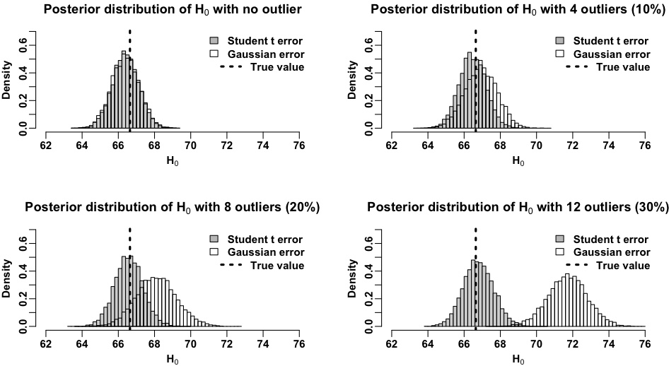
Figure 6: The resulting marginal posterior distributions of $H_{0}$ when there is no outlier (top-left), 4 outliers (top-right), 8 outliers (bottom-left), and 12 outliers (bottom-right). The vertical dashed line in each panel represents the generative true value of $H_{0}$, 66.643. It shows that the meta-analysis with Student’s $t_{4}$ error is robust to outlying inputs unlike the one with Gaussian error.

Table 2 numerically summarizes the model fits. We use the posterior mean as an $H_{0}$ estimate and posterior standard deviation as an $1\sigma$ uncertainty to be comparable with standard errors in existing works. The $H_{0}$ estimates under Student’s $t_{4}$ error remain almost the same near the true value of $H_{0}$ in all cases, while those under Gaussian error change noticeably. These changes are quantified via bias, coefficient of variation, and root mean square error. For example, when 12 time delay inputs (30%) are manipulated, the bias under Gaussian error is 7.611%, but that under Student’s $t$ error is only 0.228%. The $1\sigma$ uncertainty is also larger under Gaussian error; the coefficient of variation under Gaussian error is 1.630% and that under Student’s $t$ error is 1.251%. Its difference is not as noticeable as bias. The root mean square error under Gaussian error is more than five times larger than that under Student’s $t$ error (5.187 versus 0.848) mostly due to the contribution of bias.

Table 2: Numerical summaries obtained by fitting the meta-analysis with either Student’s $t_{4}$ error or Gaussian error. We report the posterior means (Post. mean), posterior standard deviations (sd), bias in percentage, coefficient of variation (CV) in percentage, and root mean square error (RMSE). The true value of $H_{0}$ is 66.643.

		No outliers	4 outliers (10%)	8 outliers (20%)	12 outliers (30%)
Post. mean (sd)	Gaussian	66.393 (0.761)	66.933 (0.887)	68.108 (1.115)	71.715 (1.086)
	Student’s $t_{4}$	66.406 (0.730)	66.461 (0.739)	66.581 (0.783)	66.795 (0.834)
Bias (%)	Gaussian	0.375	0.435	2.199	7.611
	Student’s $t_{4}$	0.355	0.272	0.093	0.228
CV (%)	Gaussian	1.109	1.330	1.673	1.630
	Student’s $t_{4}$	1.095	1.109	1.175	1.251
RMSE	Gaussian	0.801	0.933	1.841	5.187
	Student’s $t_{4}$	0.768	0.761	0.786	0.848

As for the computational cost of each simulation, it takes 431 seconds on average to implement 10,000 iterations for each Markov chain. The average Gelman-Rubin diagnostic statistic for $H_{0}$ is 1.0045 and the largest value for this diagnostic statistic is 1.0135 in all cases. The average effective sample size for $H_{0}$ is about 1,200 out of 25,000 posterior samples in each case. The posterior predictive checks do not show evidence that the model fails to describe the data well; see Figure 10 of Appendix for more details.

5.2 Simulated Study II

The most recent work of the STRIDES collaboration (Schmidt et al., 2023) analyzes 31 quadruply lensed systems via an automated uniform lens modeling approach that has been improved from Shajib et al. (2019). They estimate Fermat potential differences of 30 quad-lens systems (out of 31), and predict the corresponding time delays under the standard cosmological model with $\Omega=0.3$ and $H_{0}=70$. The information about the external convergence ($\kappa_{\textrm{ext},k}$’s) is not clearly specified in their simulation setting, but considering that the true value of $H_{0}$ is assumed to be completely known, zero external convergence might have been adopted. The left panel of Figure 7 shows their workflow. The observed data are colored in gray. The Fermat potential difference estimates and predicted time delays are listed in Table 8 of Schmidt et al. (2023).

We take advantage of their real-data analyses to see whether the proposed meta-analysis can accurately trace back to the true value of $H_{0}$ given their Fermat potential difference estimates and predicted time delays. To make the simulation setting more realistic, we treat the unknown external convergence in each lens system as an unknown model parameter to be estimated. The right panel of Figure 7 outlines this work. The gray circles indicate the inputs of the meta-analysis. This setting is ideal for evaluating the performance of the meta-analysis because the STRIDES collaboration has encoded the information about the cosmological parameters under the standard cosmology, such as $\Omega_{\textrm{m}}$ and $H_{0}$, into the predicted time delays.

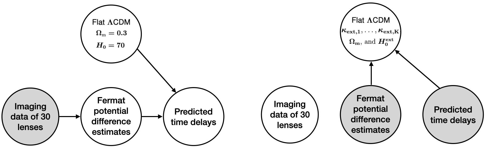
Figure 7: The left panel shows the workflow of the most recent work of the STRIDES collaboration (Schmidt et al., 2023). They analyze 31 quad-lens systems using an automated uniform lens modeling approach, reporting estimates of the Fermat potential differences from 30 quad-lens systems (out of 31). Given these estiamtes and fixed cosmological parameters under the standard cosmological model ($\Lambda$CDM), they predict time delays. The right panel shows the workflow of the proposed meta-analysis. We treat their Fermat potential difference estimates and time delay estimates as inputs to the proposed meta-analysis to see whether the meta-analysis can accurately trace back to the fixed cosmological parameters including $H_{0}$.

The default data set takes these Fermat potential difference estimates and predicted time delays as inputs. As for uncertainties of these estimates, the meta-analysis only takes a single-number uncertainty (standard error). However, the reported uncertainties in Table 8 of Schmidt et al. (2023) are 16% and 84% percentiles of a posterior distribution, and these percentiles are not always symmetric around each estimate. For example, one of the predicted time delays and its 68% uncertainty are reported as $-100^{+4.7}_{-3.0}$. To be conservative, we take the larger distance from the estimate to one of the percentiles as the input uncertainty for the meta-analysis. That means, we set the standard error of the predicted time delay to $4.7$ when $-100^{+4.7}_{-3.0}$ is reported in Table 8 of Schmidt et al. (2023). The resulting standard error still satisfies the 3% coefficient of variation level that the community expects; the median coefficient of variation in percentage is $3.018\%$ for the time delay inputs $(100\hat{\sigma}_{\Delta}/\hat{\Delta})$, and 3.030% for the Fermat potential difference inputs $(100\hat{\sigma}_{\phi}/\hat{\phi})$.

To investigate the sensitivity of the meta-analysis to outlying inputs, we set three other data sets by manipulating 9 (10%), 18 (20%), and 27 (30%) time delay inputs out of 90, respectively, as done in the previous simulation study. The inputs to be manipulated are $\Delta t_{ABk}$ for $k=1,2,\ldots,27$ in Table 8 of Schmidt et al. (2023), which corresponds to $\hat{\Delta}_{12k}$ in our notation. We contaminate these selected inputs by adding 10 times larger standard errors to the inputs. For example, the predicted time delay between lensed images $A$ and $B$ of quasar J0029-3814 with $68\%$ credible interval in Table 8 of Schmidt et al. (2023) is $-100^{+4.7}_{\small-3.0}$, which is modified to be $\hat{\Delta}_{AB1}+10\hat{\sigma}_{\Delta_{AB1}}=-100+47=-53$ and the $1\sigma$ uncertainty of this modified time delay input remains the same as 4.7.

The model fits are visualized in Figure 8. Overall, the meta-analyses with Student’s $t_{4}$ error robustly infer $H_{0}$ in all cases. The posterior distribution of $H_{0}$ under Gaussian error is not sensitive to the manipulation of 9 inputs (10%), either. However, it begins to deviate from the true value with wider spread when 18 inputs (20%) are contaminated. This might be because the increased input data size (90 input pairs in this study compared to 40 in the previous one) makes the meta-analysis under Gaussian error less sensitive to the small number of manipulated data. When 27 inputs (30%) are modified, five Markov chains under Gaussian error start exploring local modes without jumping between modes. Thus, we replace the Metropolis update for $H_{0}$ with the repelling-attracting Metropolis update to encourage the Markov chains to jump between modes. The white histogram in the bottom-right panel of Figure 8 shows the multimodal posterior distribution explored by the the repelling-attracting Metropolis within Gibbs sampler. The true value of $H_{0}$ is located near a valley between the two highest modes, meaning that the meta-analysis under Gaussian error loses its ability to capture the true value of $H_{0}$ near the highest mode.

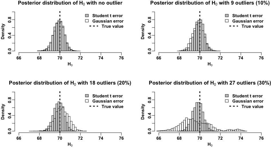
Figure 8: The resulting marginal posterior distributions of $H_{0}$ when there is no outlier (top-left), 9 outliers (top-right), 18 outliers (bottom-left), and 27 outliers (bottom-right). The vertical dashed line in each panel represents the generative true value of $H_{0}$, 70. It shows that the meta-analysis with Student’s $t_{4}$ error is robust to outlying inputs. The posterior distributions of Gaussian error starts deviating from the true value of $H_{0}$ when there are 18 outliers (20%), ending up with multiple modes in the presence of 27 outliers (30%).

Table 3: Numerical summaries obtained by fitting the meta-analysis with either Student’s $t_{4}$ error or Gaussian error. We report the posterior means (Post. mean), posterior standard deviations (sd), bias in percentage, coefficient of variation (CV) in percentage, and root mean square error (RMSE). The true value of $H_{0}$ is 70.

		No outliers	9 outliers (10%)	18 outliers (20%)	27 outliers (30%)
Post. mean (sd)	Gaussian	69.884 (0.513)	69.823 (0.543)	70.216 (0.665)	69.609 (1.509)
	Student’s $t_{4}$	69.897 (0.487)	69.921 (0.471)	69.887 (0.507 )	69.796 (0.521)
Bias (%)	Gaussian	0.166	0.253	0.308	0.559
	Student’s $t_{4}$	0.148	0.112	0.161	0.292
CV (%)	Gaussian	0.733	0.776	0.949	2.156
	Student’s $t_{4}$	0.695	0.672	0.724	0.744
RMSE	Gaussian	0.526	0.571	0.699	1.559
	Student’s $t_{4}$	0.497	0.477	0.519	0.559

Table 3 numerically summarizes the model fits. Estimates and evaluation criteria obtained by both types of error do not show notable differences even when there are 18 outlying inputs, which is consistent to the first three panels in Figure 8. In the case where we manipulate 27 input time delays (30%), bias under Gaussian error does not reflect the multimodal nature of the posterior distribution well because the posterior mean (69.609) is still near the true value (70). However, both coefficient of variation and root mean square error become about three times larger under Gaussian error due to the multimodal aspect of the resulting posterior distribution of $H_{0}$.

When it comes to the computational cost, it takes about 2,900 seconds on average to implement 10,000 iterations by the default Metropolis-Hastings within Gibbs sampler, while it takes about 3,400 seconds on average to implement repelling-attracting Metropolis within Gibbs sampler. The average Gelman-Rubin diagnostic statistic for $H_{0}$, except the multimodal case of the Gaussian error with 27 outliers, is 1.011 and the largest value for this diagnostic statistic is 1.027. In the multimodal case, the Gelam-Rubin diagnostic statistic with the default Metropolis-Hastings within Gibbs sampler is 3.629, while it reduces to 1.146 with the repelling-attracting Metropolis within Gibbs sampler. The effective sample size for $H_{0}$ under Student’s $t$ error increases from 262 (out of 25,000) to 490 as the number of outliers increases, while it decreases from 251 to 9 (23 when multimodal sampler is adopted) under Gaussian error. The posterior predictive checks do not show evidence for the lack of the model fit even for the multimodal case under Gaussian error because the posterior distribution in this case is nearly centered at the true value; see Figure 11 of Appendix for more details.

6 Realistic Data Analysis

Table 4: The Fermat potential difference and time delay estimates reported in the literature. As for quasars 2M1134-2103 and PSJ 1606-2333, we obtain $\phi_{ij}$’s, $\hat{\sigma}_{\phi_{ij}}$’s, $z_{d}$, and $z_{s}$ from Schmidt et al. (2023), and $\hat{\Delta}_{ij}$’s and $\hat{\sigma}_{\Delta_{ij}}$’s from Millon et al. (2020a). All of the information about quasar SDSS 1206+4332 is from Birrer et al. (2020).

Quasar	$z_{d}$	$z_{s}$	$i$	$j$	$\hat{\phi}_{ij}$	$\hat{\sigma}_{\phi_{ij}}$	$\hat{\Delta}_{ij}$	$\hat{\sigma}_{\Delta_{ij}}$
2M1134-2103	0.5	2.77	A	B	$-0.4707$	$0.0085$	$-30.5$	2.3
				C	$0.1825$	$0.0032$	8.6	1.5
				D	$-0.9526$	$0.0122$	-71.9	8.5
PSJ 1606-2333	0.5	1.69	A	B	$-0.2161$	$0.0042$	$-29.2$	5.1
				C	$0.1102$	$0.0024$	$-10.4$	2.3
				D	$-0.1868$	$0.0038$	$-45.7$	11.1
SDSS 1206+4332	0.745	1.789	A	B	$-0.7125$	0.0688	$-111.8$	2.7

We apply the proposed robust meta-analysis to a realistic input data set composed of three strong lens systems, 2M1134-2103, PSJ 1606-2333, and SDSS 1206+4332. The first two lens systems are quadruply-lensed quasars, meaning that we see four lensed images of each quasar in the sky. Their Fermat potential difference estimates are obtained from Table 8 of Schmidt et al. (2023) and time delay estimates are reported in Millon et al. (2020a). These two lenses have not been used to infer $H_{0}$, possibly because of their fiducial redshifts estimates of the lenses ($z_{d}$) that are arbitrarily set to 0.5 (Schmidt et al., 2023). The last system is a doubly-lensed quasar. We obtain its Fermat potential difference and time delay estimates from Birrer et al. (2019), where the Fermat potential difference estimate is not reported as a numeric value, but its posterior distribution is visualized. Thus, we set the estimate as the mode of the posterior distribution of $\phi_{AB}$, and $1\sigma$ uncertainty as the difference between the range of the posterior distribution divided by 4. These values are tabulated in Table 4.

Figure 9 shows the posterior distribution of $H_{0}$. The posterior mean and standard deviation are 75.632 and 6.918, respectively, which is 9.147% coefficient of variation in percentage. For a comparison with existing estimates in tension, we display 68% intervals on top of the distribution. The first eight intervals are based on the time delay cosmography (Bonvin et al., 2016; Birrer et al., 2019; Chen et al., 2019; Wong et al., 2020; Shajib et al., 2020; Birrer et al., 2020; Shajib et al., 2023), including this work. We denote how many lenses are used in each work. The bottom two intervals represent the $H_{0}$ estimates in tension between the early and late Universe measurements, that is, $67.4\pm 0.5$ (Planck Collaboration et al., 2020) and $73.04\pm 1.04$ (Riess et al., 2022), respectively. It turns out that the spread of the posterior distribution from this work is wide enough to encompass all of the 68% intervals, while its central location is consistent to most of the estimates from time delay cosmography and is close to the estimate from the late Universe measurement, $73.04\pm 1.04$ (Riess et al., 2022).

It is worth noting that the work of Birrer et al. (2019), whose 68% interval is $(63.7,~{}74.2)$ denoted in blue, uses only one doubly-lensed quasar, SDSS 1206+4332. This quasar is also used in this work, but the middle value of the resulting 68% interval of this work shown at the top of Figure 9 is larger than that of Birrer et al. (2019). This may be because the information about $H_{0}$ contained in SDSS 1206+4332 is averaged with the information in two other lens systems of this work. The interval of Birrer et al. (2020), colored in gray, also confirms this averaging effect because the impact of SDSS 1206+4332 is reduced when it is averaged with six other lenses, producing the larger central location.

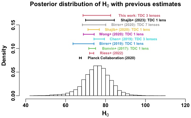
Figure 9: The resulting marginal posterior distributions of $H_{0}$ with the three strong lens systems, 2M1134-2103, PSJ 1606-2333, and SDSS 1206+4332. The posterior mean and standard deviation are 75.632 and 6.918, respectively. Its coefficient of variation in percentage is 9.147%.

The computational cost is not expensive in analyzing these three lens systems. It takes about 48 seconds on average to implement 10,000 iterations. The Gelman-Rubin diagnostic statistic for $H_{0}$ is 1.0001. The effective sample size for $H_{0}$ is 1,103 out of 25,000. From the posterior predictive check, we do not find particular evidence that the model is not sufficient to explain the data; see Figure 12 of Appendix for more details.

7 Concluding Remarks

Using time delay cosmography, we have proposed a robust meta-analysis based on Student’s $t$ error to infer the current expansion rate of the Universe, called the Hubble constant ($H_{0}$). Input data for this meta-analysis are the estimates of time delays and Fermat potential differences that can be obtained from independent studies in the literature. Thus, the meta-analysis does not need to model the time series data or high-resolution imaging data from scratch to estimate time delays and Fermat potential difference estimates, respectively. The output of this meta-analysis is posterior samples of two cosmological parameters, $H_{0}$ and $\Omega_{\textrm{m}}$, and external convergence of each lens system ($\kappa_{1},\kappa_{2},\ldots,\kappa_{K}$). Two simulation studies emphasize how robustly and accurately the proposed meta-analysis can infer $H_{0}$ in the presence of outliers. In a realistic data analysis, we apply the meta-analysis to three lens systems, two of which have never been used in estimating $H_{0}$ in the literature, and estimate $H_{0}$ by $75.632\pm 6.918$. This corresponds to 9.147% coefficient of variation ($100\hat{\sigma}_{{H}_{0}}/\hat{H}_{0}$), which is called precision level in time delay cosmography.

The biggest limitation of the meta-analysis is that the meta-analysis considers paired estimates within the same lens system (for example, in a quad-lens system) as independent observations, even though they may not be independent in reality especially within the same lens system. For example, $\hat{\Delta}_{12k}$, $\hat{\Delta}_{13k}$, and $\hat{\Delta}_{14k}$ (or $\hat{\phi}_{12k}$, $\hat{\phi}_{13k}$, and $\hat{\phi}_{14k}$) may have some physical or statistical dependence as they are estimated in the same lens system. Thus, it is more principled to model such a dependence via a multivariate Student’s $t$ distribution on $\hat{\Delta}_{12k}$, $\hat{\Delta}_{13k}$, and $\hat{\Delta}_{14k}$ and another multivariate Student’s $t$ distribution on $\hat{\phi}_{12k}$, $\hat{\phi}_{13k}$, and $\hat{\phi}_{14k}$, if the information about their correlations is available.

Another limitation is that the meta-analysis takes the Fermat potential difference estimates as inputs, while most published articles that infer $H_{0}$ via time delay cosmography do not report Fermat potential difference estimates. Instead, they report estimates of time delay distances, that is, $D_{\Delta}(H_{0},z_{k},\Omega)$ in Eqn (3), even though they must have obtained the Fermat potential difference estimates to infer the time delay distances. It is not impossible to transform the time delay distance estimate to a Fermat potential difference estimate given a time delay estimate via Eqn (1). However, such a transformation is not desirable because estimates of time delay distances already reflect the underlying cosmology including the information about an $H_{0}$ estimate, as its notation indicates. The resulting transformation inevitably encodes this information about the $H_{0}$ estimate into the Fermat potential difference estimates. Inferring $H_{0}$ from these transformed Fermat potential difference estimates will just recover the $H_{0}$ estimate used in the time delay distance estimates). Thus, it is important to obtain the Fermat potential difference estimates from high-resolution imaging data (e.g., Schmidt et al. (2023) and Ertl et al. (2023)), and independently obtain time delay estimates from multiple time series data of brightness to put them into the meta-analyses as inputs.

In the era of the Vera C. Rubin Observatory Legacy Survey of Space and Time and James Webb Space Telescope, an unprecedented number of strong lens quasars will be detected. For example, Oguri and Marshall (2010) expect that the Rubin Observatory will detect thousands of lensed quasars. It is worth noting that one of the recent $H_{0}$ estimates via time delay cosmography uses only seven lens systems (Birrer et al., 2020). Birrer and Treu (2021) point out that time delay cosmography with a set of 40 time delay lens systems and their spatially resolved stellar kinematic information will be able to achieve 1.5% precision level of the $H_{0}$ estimate. Thus time delay cosmography will contribute to understanding the current tension better as their long-term time series data become available in a decade. However, analyzing time series data and imaging data of thousands of strong lens systems from scratch may require even more substantial human efforts than analyzing seven lenses. The proposed meta-analysis will be useful in this case as it produces a robust benchmark estimate of $H_{0}$ without requiring the analyses of time series and imaging data from scratch.

Posterior Predictive Checks

We derive the posterior predictive distribution $q$ of the predicted input data given the observed input data as follows. Here, we denote predicted values of Fermat potential difference and time delay inputs as $\hat{\phi}_{ijk}^{\ast}$ and $\hat{\Delta}_{ijk}^{\ast}$, respectively, and collectively denote the model parameters as $\theta=(H_{0},\Omega,\kappa_{\text{ext}})$. The posterior predictive density function is

$$q(\hat{\phi}_{ijk}^{\ast},\hat{\Delta}_{ijk}^{\ast}\mid\hat{\phi}_{ijk},\hat{\Delta}_{ijk})=\int w(\hat{\phi}_{ijk}^{\ast},\hat{\Delta}_{ijk}^{\ast}\mid\theta)~{}\pi(\theta\mid\hat{\phi}_{ijk},\hat{\Delta}_{ijk})~{}d\theta.$$ (15)

The posterior density function $\pi(\theta\mid\hat{\phi}_{ijk},\hat{\Delta}_{ijk})$ is already defined in Eqn (14), the density of the predicted input data given the model parameters $w(\hat{\phi}_{ijk}^{\ast},\hat{\Delta}_{ijk}^{\ast}\mid\theta)$ can be obtained by replacing $(\hat{\phi}_{ijk},\hat{\Delta}_{ijk})$ with $(\hat{\phi}_{ijk}^{\ast},\hat{\Delta}_{ijk}^{\ast})$ from $L(\theta)$ in Eqn (12).

One way to simulate this posterior predictive distribution is to (i) draw a random sample of $\theta$ from $\pi(\theta\mid\hat{\phi}_{ijk},\hat{\Delta}_{ijk})$, (ii) generate a random sample of $(\hat{\phi}_{ijk}^{\ast},\hat{\Delta}_{ijk}^{\ast})$ from $w(\hat{\phi}_{ijk}^{\ast},\hat{\Delta}_{ijk}^{\ast}\mid\theta)$ given the previously sampled $\theta$, and (iii) repeat the previous two sampling steps. As for Step (i), we treat the combined MCMC sample of size 25,000 obtained in each example as 25,000 draws from $\pi(\theta\mid\hat{\phi}_{ijk},\hat{\Delta}_{ijk})$. In Step (ii), it is not straightforward to sample the pair $(\hat{\phi}_{ijk}^{\ast},\hat{\Delta}_{ijk}^{\ast})$ from the joint distribution $w$ directly. However, it is simple to sample their two conditionals, that is, $w_{1}(\hat{\phi}_{ijk}^{\ast}\mid\theta,\hat{\Delta}_{ijk}^{\ast})$ and $w_{2}(\hat{\Delta}_{ijk}^{\ast}\mid\theta,\hat{\phi}_{ijk}^{\ast})$, because these conditionals are Student’s $t_{4}$ distributions. The conditional distribution of $\hat{\phi}_{ijk}^{\ast}$ given $(\theta,\hat{\Delta}_{ijk}^{\ast})$ can be obtained by replacing $(\hat{\phi}_{ijk},\hat{\Delta}_{ijk})$ with $(\hat{\phi}_{ijk}^{\ast},\hat{\Delta}_{ijk}^{\ast})$ in Eqn (13). The conditional distribution of $\hat{\Delta}_{ijk}^{\ast}$ given $(\theta,\hat{\phi}_{ijk}^{\ast})$ is

$$\hat{\Delta}^{\ast}_{ijk}\mid\theta,\hat{\phi}_{ijk}^{\ast}\sim t_{4}\!\left(\frac{D_{\Delta}(H_{0},z_{k},\Omega)\hat{\phi}_{ijk}^{\ast}}{(1-\kappa_{\text{ext},k})c},~{}~{}\sqrt{\frac{D_{\Delta}(H_{0},z_{k},\Omega)^{2}\hat{\sigma}^{2}_{\phi_{ijk}}}{(1-\kappa_{\text{ext},k})^{2}c^{2}}+\hat{\sigma}^{2}_{\Delta_{ijk}}}~{}~{}\right).$$ (16)

Adopting the idea of Gibbs sampling, we repeatedly sample these two conditionals 30 times given each sample of $\theta$, and take only the last (30th) pair as a sample of $(\hat{\phi}_{ijk}^{\ast},\hat{\Delta}_{ijk}^{\ast})$ from $w(\hat{\phi}_{ijk}^{\ast},\hat{\Delta}_{ijk}^{\ast}\mid\theta)$ given each sample of $\theta$.

We repeat these two steps, (i) and (ii), 5,000 times and investigate the posterior predictive distribution in light of the observed input data. Specifically we check whether the observed input data are noticeably distant from the center of the posterior predictive distribution because it can be evidence that the model does not describe the data well.

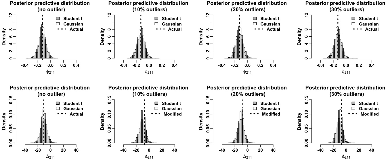
Figure 10: The first row displays posterior predictive distributions of the first Fermat potential difference input obtained by Student’s $t_{4}$ error (in gray) and Gaussian error (in white). The second row exhibits those of the first time delay input. Each column represents one of the four cases (no outlier, 10% outliers, 20% outliers, and 30% outliers). Each panel denotes the actual input or modified input (to be an outlier) by the vertical dashed line.

For the meta-analysis based on Gaussian error, we can obtain the conditional distributions $w_{1}$ and $w_{2}$ by simply replacing $t_{4}$ with $N$ in Eqns (13) and (16). The other sampling details are the same as before.

Figure 10 displays the posterior predictive distributions of the first input pair obtained by fitting the model with either Student’s $t$ (in gray) or Gaussian error (in white) for each of the four cases of Section 5.1. Each column represents different cases (no outlier, 10%, 20% and 30% outliers from the left), containing the posterior predictive distribution of the first Fermat potential difference input (top) and that of the first time delay input (bottom). For reference, the first time delay input has been modified to be an outlier in the last three cases (with outliers). The vertical lines indicate the observed input data. Overall, the posterior predictive distributions obtained with Student’s $t$ error have wider spread than those obtained with Gaussian error due to the heavy-tailed feature of Student’s $t$ error. Also, the first observed Fermat potential difference and time delay inputs are located near the modes of their posterior predictive distributions in all cases. Even though the modes of the posterior predictive distributions of the time delay input (second row) slightly move to the left as the number of outliers increases, the observed time delay input is still close to the mode.

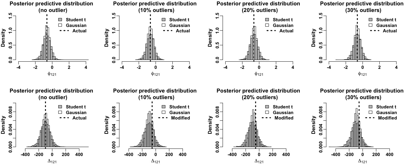
Figure 11: The first row displays posterior predictive distributions of the first Fermat potential difference input obtained by Student’s $t_{4}$ error (in gray) and Gaussian error (in white). The second row exhibits those of the first time delay input. Each column represents one of the four cases (no outlier, 10% outliers, 20% outliers, and 30% outliers). Each panel denotes the actual input or modified input (to be an outlier) by the vertical dashed line.

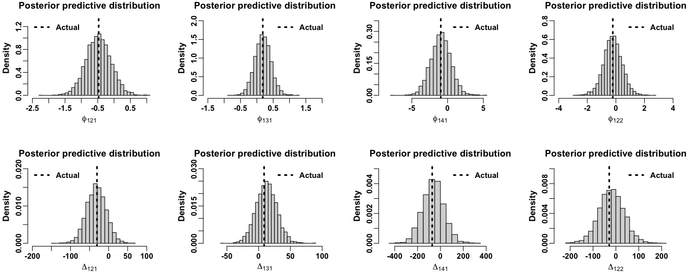
Figure 12: The first row displays posterior predictive distributions of the first four Fermat potential difference inputs obtained by Student’s $t_{4}$ error (in gray) and Gaussian error (in white). The second row exhibits those of the first four time delay inputs. Each panel denotes the observed input by the vertical dashed line.

Figure 11 similarly summarizes the posterior predictive distributions of the first input pair used in the second simulation study in Section 5.2. The outcomes are similar to the previous ones, and these provide empirical evidence that the model predicts the data well.

Figure 12 exhibits the posterior predictive distributions of the first four Fermat potential difference (top) and time delay (bottom) inputs used in Section 6. Each column corresponds to a different input pair (1st, 2nd, 3rd, or 4th pair from the left). Overall, the observed inputs are located near the center of the posterior predictive distributions.

[Acknowledgments] HT appreciates Michael Fleck, a multimedia specialist in the department of statistics at Pennsylvania State University, for creating the image in the left panel of Figure 1. XD acknowledges the support from the World Premier International Research Center Initiative (WPI) in Japan. We thank Simon Birrer for his productive comments on this manuscript.

The data and R code The R code, standalone.R, contains all of the data sets used in the three numerical examples and reproduces all of the results reported in this work. The same results can be obtained by using the R package, h0.

References

- Abdalla et al. (2022) {barticle}[author] \bauthor\bsnmAbdalla, \bfnmElcio\binitsE., \bauthor\bsnmAbellán, \bfnmGuillermo Franco\binitsG. F., \bauthor\bsnmAboubrahim, \bfnmAmin\binitsA., \bauthor\bsnmAgnello, \bfnmAdriano\binitsA., \bauthor\bsnmAkarsu, \bfnmÖzgür\binitsÖ., \bauthor\bsnmAkrami, \bfnmYashar\binitsY., \bauthor\bsnmAlestas, \bfnmGeorge\binitsG., \bauthor\bsnmAloni, \bfnmDaniel\binitsD., \bauthor\bsnmAmendola, \bfnmLuca\binitsL., \bauthor\bsnmAnchordoqui, \bfnmLuis A.\binitsL. A., \bauthor\bsnmAnderson, \bfnmRichard I.\binitsR. I., \bauthor\bsnmArendse, \bfnmNikki\binitsN., \bauthor\bsnmAsgari, \bfnmMarika\binitsM., \bauthor\bsnmBallardini, \bfnmMario\binitsM., \bauthor\bsnmBarger, \bfnmVernon\binitsV., \bauthor\bsnmBasilakos, \bfnmSpyros\binitsS., \bauthor\bsnmBatista, \bfnmRonaldo C.\binitsR. C., \bauthor\bsnmBattistelli, \bfnmElia S.\binitsE. S., \bauthor\bsnmBattye, \bfnmRichard\binitsR., \bauthor\bsnmBenetti, \bfnmMicol\binitsM., \bauthor\bsnmBenisty, \bfnmDavid\binitsD., \bauthor\bsnmBerlin, \bfnmAsher\binitsA., \bauthor\bsnmde Bernardis, \bfnmPaolo\binitsP., \bauthor\bsnmBerti, \bfnmEmanuele\binitsE., \bauthor\bsnmBidenko, \bfnmBohdan\binitsB., \bauthor\bsnmBirrer, \bfnmSimon\binitsS., \bauthor\bsnmBlakeslee, \bfnmJohn P.\binitsJ. P., \bauthor\bsnmBoddy, \bfnmKimberly K.\binitsK. K., \bauthor\bsnmBom, \bfnmClecio R.\binitsC. R., \bauthor\bsnmBonilla, \bfnmAlexander\binitsA., \bauthor\bsnmBorghi, \bfnmNicola\binitsN., \bauthor\bsnmBouchet, \bfnmFrançois R.\binitsF. R., \bauthor\bsnmBraglia, \bfnmMatteo\binitsM., \bauthor\bsnmBuchert, \bfnmThomas\binitsT., \bauthor\bsnmBuckley-Geer, \bfnmElizabeth\binitsE., \bauthor\bsnmCalabrese, \bfnmErminia\binitsE., \bauthor\bsnmCaldwell, \bfnmRobert R.\binitsR. R., \bauthor\bsnmCamarena, \bfnmDavid\binitsD., \bauthor\bsnmCapozziello, \bfnmSalvatore\binitsS., \bauthor\bsnmCasertano, \bfnmStefano\binitsS., \bauthor\bsnmChen, \bfnmGeoff C. F.\binitsG. C. F., \bauthor\bsnmChluba, \bfnmJens\binitsJ., \bauthor\bsnmChen, \bfnmAngela\binitsA., \bauthor\bsnmChen, \bfnmHsin-Yu\binitsH.-Y., \bauthor\bsnmChudaykin, \bfnmAnton\binitsA., \bauthor\bsnmCicoli, \bfnmMichele\binitsM., \bauthor\bsnmCopi, \bfnmCraig J.\binitsC. J., \bauthor\bsnmCourbin, \bfnmFred\binitsF., \bauthor\bsnmCyr-Racine, \bfnmFrancis-Yan\binitsF.-Y., \bauthor\bsnmCzerny, \bfnmBożena\binitsB., \bauthor\bsnmDainotti, \bfnmMaria\binitsM., \bauthor\bsnmD’Amico, \bfnmGuido\binitsG., \bauthor\bsnmDavis, \bfnmAnne-Christine\binitsA.-C., \bauthor\bsnmde Cruz Pérez, \bfnmJavier\binitsJ., \bauthor\bsnmde Haro, \bfnmJaume\binitsJ., \bauthor\bsnmDelabrouille, \bfnmJacques\binitsJ., \bauthor\bsnmDenton, \bfnmPeter B.\binitsP. B., \bauthor\bsnmDhawan, \bfnmSuhail\binitsS., \bauthor\bsnmDienes, \bfnmKeith R.\binitsK. R., \bauthor\bsnmDi Valentino, \bfnmEleonora\binitsE., \bauthor\bsnmDu, \bfnmPu\binitsP., \bauthor\bsnmEckert, \bfnmDominique\binitsD., \bauthor\bsnmEscamilla-Rivera, \bfnmCelia\binitsC., \bauthor\bsnmFerté, \bfnmAgnès\binitsA., \bauthor\bsnmFinelli, \bfnmFabio\binitsF., \bauthor\bsnmFosalba, \bfnmPablo\binitsP., \bauthor\bsnmFreedman, \bfnmWendy L.\binitsW. L., \bauthor\bsnmFrusciante, \bfnmNoemi\binitsN., \bauthor\bsnmGaztañaga, \bfnmEnrique\binitsE., \bauthor\bsnmGiarè, \bfnmWilliam\binitsW., \bauthor\bsnmGiusarma, \bfnmElena\binitsE., \bauthor\bsnmGómez-Valent, \bfnmAdrià\binitsA., \bauthor\bsnmHandley, \bfnmWill\binitsW., \bauthor\bsnmHarrison, \bfnmIan\binitsI., \bauthor\bsnmHart, \bfnmLuke\binitsL., \bauthor\bsnmHazra, \bfnmDhiraj Kumar\binitsD. K., \bauthor\bsnmHeavens, \bfnmAlan\binitsA., \bauthor\bsnmHeinesen, \bfnmAsta\binitsA., \bauthor\bsnmHildebrandt, \bfnmHendrik\binitsH., \bauthor\bsnmHill, \bfnmJ. Colin\binitsJ. C., \bauthor\bsnmHogg, \bfnmNatalie B.\binitsN. B., \bauthor\bsnmHolz, \bfnmDaniel E.\binitsD. E., \bauthor\bsnmHooper, \bfnmDeanna C.\binitsD. C., \bauthor\bsnmHosseininejad, \bfnmNikoo\binitsN., \bauthor\bsnmHuterer, \bfnmDragan\binitsD., \bauthor\bsnmIshak, \bfnmMustapha\binitsM., \bauthor\bsnmIvanov, \bfnmMikhail M.\binitsM. M., \bauthor\bsnmJaffe, \bfnmAndrew H.\binitsA. H., \bauthor\bsnmJang, \bfnmIn Sung\binitsI. S., \bauthor\bsnmJedamzik, \bfnmKarsten\binitsK., \bauthor\bsnmJimenez, \bfnmRaul\binitsR., \bauthor\bsnmJoseph, \bfnmMelissa\binitsM., \bauthor\bsnmJoudaki, \bfnmShahab\binitsS., \bauthor\bsnmKamionkowski, \bfnmMarc\binitsM., \bauthor\bsnmKarwal, \bfnmTanvi\binitsT., \bauthor\bsnmKazantzidis, \bfnmLavrentios\binitsL., \bauthor\bsnmKeeley, \bfnmRyan E.\binitsR. E., \bauthor\bsnmKlasen, \bfnmMichael\binitsM., \bauthor\bsnmKomatsu, \bfnmEiichiro\binitsE., \bauthor\bsnmKoopmans, \bfnmLéon V. E.\binitsL. V. E., \bauthor\bsnmKumar, \bfnmSuresh\binitsS., \bauthor\bsnmLamagna, \bfnmLuca\binitsL., \bauthor\bsnmLazkoz, \bfnmRuth\binitsR., \bauthor\bsnmLee, \bfnmChung-Chi\binitsC.-C., \bauthor\bsnmLesgourgues, \bfnmJulien\binitsJ., \bauthor\bsnmLevi Said, \bfnmJackson\binitsJ., \bauthor\bsnmLewis, \bfnmTiffany R.\binitsT. R., \bauthor\bsnmL’Huillier, \bfnmBenjamin\binitsB., \bauthor\bsnmLucca, \bfnmMatteo\binitsM., \bauthor\bsnmMaartens, \bfnmRoy\binitsR., \bauthor\bsnmMacri, \bfnmLucas M.\binitsL. M., \bauthor\bsnmMarfatia, \bfnmDanny\binitsD., \bauthor\bsnmMarra, \bfnmValerio\binitsV., \bauthor\bsnmMartins, \bfnmCarlos J. A. P.\binitsC. J. A. P., \bauthor\bsnmMasi, \bfnmSilvia\binitsS., \bauthor\bsnmMatarrese, \bfnmSabino\binitsS., \bauthor\bsnmMazumdar, \bfnmArindam\binitsA., \bauthor\bsnmMelchiorri, \bfnmAlessandro\binitsA., \bauthor\bsnmMena, \bfnmOlga\binitsO., \bauthor\bsnmMersini-Houghton, \bfnmLaura\binitsL., \bauthor\bsnmMertens, \bfnmJames\binitsJ., \bauthor\bsnmMilaković, \bfnmDinko\binitsD., \bauthor\bsnmMinami, \bfnmYuto\binitsY., \bauthor\bsnmMiranda, \bfnmVivian\binitsV., \bauthor\bsnmMoreno-Pulido, \bfnmCristian\binitsC., \bauthor\bsnmMoresco, \bfnmMichele\binitsM., \bauthor\bsnmMota, \bfnmDavid F.\binitsD. F., \bauthor\bsnmMottola, \bfnmEmil\binitsE., \bauthor\bsnmMozzon, \bfnmSimone\binitsS., \bauthor\bsnmMuir, \bfnmJessica\binitsJ., \bauthor\bsnmMukherjee, \bfnmAnkan\binitsA., \bauthor\bsnmMukherjee, \bfnmSuvodip\binitsS., \bauthor\bsnmNaselsky, \bfnmPavel\binitsP., \bauthor\bsnmNath, \bfnmPran\binitsP., \bauthor\bsnmNesseris, \bfnmSavvas\binitsS., \bauthor\bsnmNiedermann, \bfnmFlorian\binitsF., \bauthor\bsnmNotari, \bfnmAlessio\binitsA., \bauthor\bsnmNunes, \bfnmRafael C.\binitsR. C., \bauthor\bsnmÓ Colgáin, \bfnmEoin\binitsE., \bauthor\bsnmOwens, \bfnmKayla A.\binitsK. A., \bauthor\bsnmÖzülker, \bfnmEmre\binitsE., \bauthor\bsnmPace, \bfnmFrancesco\binitsF., \bauthor\bsnmPaliathanasis, \bfnmAndronikos\binitsA., \bauthor\bsnmPalmese, \bfnmAntonella\binitsA., \bauthor\bsnmPan, \bfnmSupriya\binitsS., \bauthor\bsnmPaoletti, \bfnmDaniela\binitsD., \bauthor\bsnmPerez Bergliaffa, \bfnmSantiago E.\binitsS. E., \bauthor\bsnmPerivolaropoulos, \bfnmLeandros\binitsL., \bauthor\bsnmPesce, \bfnmDominic W.\binitsD. W., \bauthor\bsnmPettorino, \bfnmValeria\binitsV., \bauthor\bsnmPhilcox, \bfnmOliver H. E.\binitsO. H. E., \bauthor\bsnmPogosian, \bfnmLevon\binitsL., \bauthor\bsnmPoulin, \bfnmVivian\binitsV., \bauthor\bsnmPoulot, \bfnmGaspard\binitsG., \bauthor\bsnmRaveri, \bfnmMarco\binitsM., \bauthor\bsnmReid, \bfnmMark J.\binitsM. J., \bauthor\bsnmRenzi, \bfnmFabrizio\binitsF., \bauthor\bsnmRiess, \bfnmAdam G.\binitsA. G., \bauthor\bsnmSabla, \bfnmVivian I.\binitsV. I., \bauthor\bsnmSalucci, \bfnmPaolo\binitsP., \bauthor\bsnmSalzano, \bfnmVincenzo\binitsV., \bauthor\bsnmSaridakis, \bfnmEmmanuel N.\binitsE. N., \bauthor\bsnmSathyaprakash, \bfnmBangalore S.\binitsB. S., \bauthor\bsnmSchmaltz, \bfnmMartin\binitsM., \bauthor\bsnmSchöneberg, \bfnmNils\binitsN., \bauthor\bsnmScolnic, \bfnmDan\binitsD., \bauthor\bsnmSen, \bfnmAnjan A.\binitsA. A., \bauthor\bsnmSehgal, \bfnmNeelima\binitsN., \bauthor\bsnmShafieloo, \bfnmArman\binitsA., \bauthor\bsnmSheikh-Jabbari, \bfnmM. M.\binitsM. M., \bauthor\bsnmSilk, \bfnmJoseph\binitsJ., \bauthor\bsnmSilvestri, \bfnmAlessandra\binitsA., \bauthor\bsnmSkara, \bfnmFoteini\binitsF., \bauthor\bsnmSloth, \bfnmMartin S.\binitsM. S., \bauthor\bsnmSoares-Santos, \bfnmMarcelle\binitsM., \bauthor\bsnmSolà Peracaula, \bfnmJoan\binitsJ., \bauthor\bsnmSongsheng, \bfnmYu-Yang\binitsY.-Y., \bauthor\bsnmSoriano, \bfnmJorge F.\binitsJ. F., \bauthor\bsnmStaicova, \bfnmDenitsa\binitsD., \bauthor\bsnmStarkman, \bfnmGlenn D.\binitsG. D., \bauthor\bsnmSzapudi, \bfnmIstván\binitsI., \bauthor\bsnmTeixeira, \bfnmElsa M.\binitsE. M., \bauthor\bsnmThomas, \bfnmBrooks\binitsB., \bauthor\bsnmTreu, \bfnmTommaso\binitsT., \bauthor\bsnmTrott, \bfnmEmery\binitsE., \bauthor\bsnmvan de Bruck, \bfnmCarsten\binitsC., \bauthor\bsnmVazquez, \bfnmJ. Alberto\binitsJ. A., \bauthor\bsnmVerde, \bfnmLicia\binitsL., \bauthor\bsnmVisinelli, \bfnmLuca\binitsL., \bauthor\bsnmWang, \bfnmDeng\binitsD., \bauthor\bsnmWang, \bfnmJian-Min\binitsJ.-M., \bauthor\bsnmWang, \bfnmShao-Jiang\binitsS.-J., \bauthor\bsnmWatkins, \bfnmRichard\binitsR., \bauthor\bsnmWatson, \bfnmScott\binitsS., \bauthor\bsnmWebb, \bfnmJohn K.\binitsJ. K., \bauthor\bsnmWeiner, \bfnmNeal\binitsN., \bauthor\bsnmWeltman, \bfnmAmanda\binitsA., \bauthor\bsnmWitte, \bfnmSamuel J.\binitsS. J., \bauthor\bsnmWojtak, \bfnmRadosław\binitsR., \bauthor\bsnmYadav, \bfnmAnil Kumar\binitsA. K., \bauthor\bsnmYang, \bfnmWeiqiang\binitsW., \bauthor\bsnmZhao, \bfnmGong-Bo\binitsG.-B. and \bauthor\bsnmZumalacárregui, \bfnmMiguel\binitsM. (\byear2022). \btitleCosmology intertwined: A review of the particle physics, astrophysics, and cosmology associated with the cosmological tensions and anomalies. \bjournalJournal of High Energy Astrophysics \bvolume34 \bpages49-211. \bdoi10.1016/j.jheap.2022.04.002 \endbibitem
- Berger, Liseo and Wolpert (1999) {barticle}[author] \bauthor\bsnmBerger, \bfnmJames O.\binitsJ. O., \bauthor\bsnmLiseo, \bfnmBrunero\binitsB. and \bauthor\bsnmWolpert, \bfnmRobert L.\binitsR. L. (\byear1999). \btitleIntegrated likelihood methods for eliminating nuisance parameters. \bjournalStatistical Science \bvolume14 \bpages1 – 28. \bdoi10.1214/ss/1009211804 \endbibitem
- Birrer, Amara and Refregier (2016) {barticle}[author] \bauthor\bsnmBirrer, \bfnmSimon\binitsS., \bauthor\bsnmAmara, \bfnmAdam\binitsA. and \bauthor\bsnmRefregier, \bfnmAlexandre\binitsA. (\byear2016). \btitleThe mass-sheet degeneracy and time-delay cosmography: analysis of the strong lens RXJ1131-1231. \bjournalJournal of Cosmology and Astroparticle Physics \bvolume2016 \bpages020. \bdoi10.1088/1475-7516/2016/08/020 \endbibitem
- Birrer and Amara (2018) {barticle}[author] \bauthor\bsnmBirrer, \bfnmS.\binitsS. and \bauthor\bsnmAmara, \bfnmA.\binitsA. (\byear2018). \btitlelenstronomy: Multi-purpose gravitational lens modelling software package. \bjournalPhysics of the Dark Universe \bvolume22 \bpages189-201. \bdoi10.1016/j.dark.2018.11.002 \endbibitem
- Birrer and Treu (2021) {barticle}[author] \bauthor\bsnmBirrer, \bfnmSimon\binitsS. and \bauthor\bsnmTreu, \bfnmTommaso\binitsT. (\byear2021). \btitleTDCOSMO. V. Strategies for precise and accurate measurements of the Hubble constant with strong lensing. \bjournalAstronomy & Astrophysics \bvolume649 \bpagesA61. \bdoi10.1051/0004-6361/202039179 \endbibitem
- Birrer et al. (2019) {barticle}[author] \bauthor\bsnmBirrer, \bfnmS.\binitsS., \bauthor\bsnmTreu, \bfnmT.\binitsT., \bauthor\bsnmRusu, \bfnmC. E.\binitsC. E., \bauthor\bsnmBonvin, \bfnmV.\binitsV., \bauthor\bsnmFassnacht, \bfnmC. D.\binitsC. D., \bauthor\bsnmChan, \bfnmJ. H. H.\binitsJ. H. H. \betalet al. (\byear2019). \btitleH0LiCOW – IX. Cosmographic analysis of the doubly imaged quasar SDSS 1206+4332 and a new measurement of the Hubble constant. \bjournalMonthly Notices of the Royal Astronomical Society \bvolume484 \bpages4726-4753. \bdoi10.1093/mnras/stz200 \endbibitem
- Birrer et al. (2020) {barticle}[author] \bauthor\bsnmBirrer, \bfnmS.\binitsS., \bauthor\bsnmShajib, \bfnmA. J.\binitsA. J., \bauthor\bsnmGalan, \bfnmA.\binitsA., \bauthor\bsnmMillon, \bfnmM.\binitsM., \bauthor\bsnmTreu, \bfnmT.\binitsT., \bauthor\bsnmAgnello, \bfnmA.\binitsA. \betalet al. (\byear2020). \btitleTDCOSMO. IV. Hierarchical time-delay cosmography – joint inference of the Hubble constant and galaxy density profiles. \bjournalAstronomy & Astrophysics \bvolume643 \bpagesA165. \bdoi10.1051/0004-6361/202038861 \endbibitem
- Birrer et al. (2021) {barticle}[author] \bauthor\bsnmBirrer, \bfnmSimon\binitsS., \bauthor\bsnmShajib, \bfnmAnowar J.\binitsA. J., \bauthor\bsnmGilman, \bfnmDaniel\binitsD., \bauthor\bsnmGalan, \bfnmAymeric\binitsA., \bauthor\bsnmAalbers, \bfnmJelle\binitsJ., \bauthor\bsnmMillon, \bfnmMartin\binitsM., \bauthor\bsnmMorgan, \bfnmRobert\binitsR., \bauthor\bsnmPagano, \bfnmGiulia\binitsG., \bauthor\bsnmPark, \bfnmJi Won\binitsJ. W., \bauthor\bsnmTeodori, \bfnmLuca\binitsL., \bauthor\bsnmTessore, \bfnmNicolas\binitsN., \bauthor\bsnmUeland, \bfnmMadison\binitsM., \bauthor\bparticlede \bsnmVyvere, \bfnmLyne Van\binitsL. V., \bauthor\bsnmWagner-Carena, \bfnmSebastian\binitsS., \bauthor\bsnmWempe, \bfnmEwoud\binitsE., \bauthor\bsnmYang, \bfnmLilan\binitsL., \bauthor\bsnmDing, \bfnmXuheng\binitsX., \bauthor\bsnmSchmidt, \bfnmThomas\binitsT., \bauthor\bsnmSluse, \bfnmDominique\binitsD., \bauthor\bsnmZhang, \bfnmMing\binitsM. and \bauthor\bsnmAmara, \bfnmAdam\binitsA. (\byear2021). \btitlelenstronomy II: A gravitational lensing software ecosystem. \bjournalJournal of Open Source Software \bvolume6 \bpages3283. \bdoi10.21105/joss.03283 \endbibitem
- Birrer et al. (2022) {barticle}[author] \bauthor\bsnmBirrer, \bfnmS.\binitsS., \bauthor\bsnmMillon, \bfnmM.\binitsM., \bauthor\bsnmSluse, \bfnmD.\binitsD., \bauthor\bsnmShajib, \bfnmA. J.\binitsA. J., \bauthor\bsnmCourbin, \bfnmF.\binitsF., \bauthor\bsnmKoopmans, \bfnmL. V. E.\binitsL. V. E., \bauthor\bsnmSuyu, \bfnmS. H.\binitsS. H. and \bauthor\bsnmTreu, \bfnmT.\binitsT. (\byear2022). \btitleTime-Delay Cosmography: Measuring the Hubble Constant and other cosmological parameters with strong gravitational lensing. \bjournalarXiv e-prints \bpagesarXiv:2210.10833. \bdoi10.48550/arXiv.2210.10833 \endbibitem
- Bonvin et al. (2016) {barticle}[author] \bauthor\bsnmBonvin, \bfnmV.\binitsV., \bauthor\bsnmCourbin, \bfnmF.\binitsF., \bauthor\bsnmSuyu, \bfnmS. H.\binitsS. H., \bauthor\bsnmMarshall, \bfnmP. J.\binitsP. J., \bauthor\bsnmRusu, \bfnmC. E.\binitsC. E., \bauthor\bsnmSluse, \bfnmD.\binitsD. \betalet al. (\byear2016). \btitleH0LiCOW V. New COSMOGRAIL time delays of HE 0435–1223: to 3.8 per cent precision from strong lensing in a flat CDM model. \bjournalMonthly Notices of the Royal Astronomical Society \bvolume465 \bpages4914-4930. \bdoi10.1093/mnras/stw3006 \endbibitem
- Bonvin et al. (2018) {barticle}[author] \bauthor\bsnmBonvin, \bfnmV.\binitsV., \bauthor\bsnmChan, \bfnmJ. H. H.\binitsJ. H. H., \bauthor\bsnmMillon, \bfnmM.\binitsM., \bauthor\bsnmRojas, \bfnmK.\binitsK., \bauthor\bsnmCourbin, \bfnmF.\binitsF., \bauthor\bsnmChen, \bfnmG. C. F.\binitsG. C. F. \betalet al. (\byear2018). \btitleCOSMOGRAIL - XVII. Time delays for the quadruply imaged quasar PG 1115+080. \bjournalAstronomy & Astrophysics \bvolume616 \bpagesA183. \bdoi10.1051/0004-6361/201833287 \endbibitem
- Bonvin et al. (2019) {barticle}[author] \bauthor\bsnmBonvin, \bfnmV.\binitsV., \bauthor\bsnmMillon, \bfnmM.\binitsM., \bauthor\bsnmChan, \bfnmJ. H. H.\binitsJ. H. H., \bauthor\bsnmCourbin, \bfnmF.\binitsF., \bauthor\bsnmRusu, \bfnmC. E.\binitsC. E., \bauthor\bsnmSluse, \bfnmD.\binitsD. \betalet al. (\byear2019). \btitleCOSMOGRAIL - XVIII. time delays of the quadruply lensed quasar WFI2033-4723. \bjournalAstronomy & Astrophysics \bvolume629 \bpagesA97. \bdoi10.1051/0004-6361/201935921 \endbibitem
- Buckley-Geer et al. (2020) {barticle}[author] \bauthor\bsnmBuckley-Geer, \bfnmE. J.\binitsE. J., \bauthor\bsnmLin, \bfnmH.\binitsH., \bauthor\bsnmRusu, \bfnmC. E.\binitsC. E., \bauthor\bsnmPoh, \bfnmJ.\binitsJ., \bauthor\bsnmPalmese, \bfnmA.\binitsA., \bauthor\bsnmAgnello, \bfnmA.\binitsA., \bauthor\bsnmChristensen, \bfnmL.\binitsL., \bauthor\bsnmFrieman, \bfnmJ.\binitsJ., \bauthor\bsnmShajib, \bfnmA. J.\binitsA. J., \bauthor\bsnmTreu, \bfnmT.\binitsT., \bauthor\bsnmCollett, \bfnmT.\binitsT., \bauthor\bsnmBirrer, \bfnmS.\binitsS., \bauthor\bsnmAnguita, \bfnmT.\binitsT., \bauthor\bsnmFassnacht, \bfnmC. D.\binitsC. D., \bauthor\bsnmMeylan, \bfnmG.\binitsG., \bauthor\bsnmMukherjee, \bfnmS.\binitsS., \bauthor\bsnmWong, \bfnmK. C.\binitsK. C., \bauthor\bsnmAguena, \bfnmM.\binitsM., \bauthor\bsnmAllam, \bfnmS.\binitsS., \bauthor\bsnmAvila, \bfnmS.\binitsS., \bauthor\bsnmBertin, \bfnmE.\binitsE., \bauthor\bsnmBhargava, \bfnmS.\binitsS., \bauthor\bsnmBrooks, \bfnmD.\binitsD., \bauthor\bsnmCarnero Rosell, \bfnmA.\binitsA., \bauthor\bsnmCarrasco Kind, \bfnmM.\binitsM., \bauthor\bsnmCarretero, \bfnmJ.\binitsJ., \bauthor\bsnmCastander, \bfnmF. J.\binitsF. J., \bauthor\bsnmCostanzi, \bfnmM.\binitsM., \bauthor\bsnmda Costa, \bfnmL. N.\binitsL. N., \bauthor\bsnmDe Vicente, \bfnmJ.\binitsJ., \bauthor\bsnmDesai, \bfnmS.\binitsS., \bauthor\bsnmDiehl, \bfnmH. T.\binitsH. T., \bauthor\bsnmDoel, \bfnmP.\binitsP., \bauthor\bsnmEifler, \bfnmT. F.\binitsT. F., \bauthor\bsnmEverett, \bfnmS.\binitsS., \bauthor\bsnmFlaugher, \bfnmB.\binitsB., \bauthor\bsnmFosalba, \bfnmP.\binitsP., \bauthor\bsnmGarcía-Bellido, \bfnmJ.\binitsJ., \bauthor\bsnmGaztanaga, \bfnmE.\binitsE., \bauthor\bsnmGruen, \bfnmD.\binitsD., \bauthor\bsnmGruendl, \bfnmR. A.\binitsR. A., \bauthor\bsnmGschwend, \bfnmJ.\binitsJ., \bauthor\bsnmGutierrez, \bfnmG.\binitsG., \bauthor\bsnmHinton, \bfnmS. R.\binitsS. R., \bauthor\bsnmHonscheid, \bfnmK.\binitsK., \bauthor\bsnmJames, \bfnmD. J.\binitsD. J., \bauthor\bsnmKuehn, \bfnmK.\binitsK., \bauthor\bsnmKuropatkin, \bfnmN.\binitsN., \bauthor\bsnmMaia, \bfnmM. A. G.\binitsM. A. G., \bauthor\bsnmMarshall, \bfnmJ. L.\binitsJ. L., \bauthor\bsnmMelchior, \bfnmP.\binitsP., \bauthor\bsnmMenanteau, \bfnmF.\binitsF., \bauthor\bsnmMiquel, \bfnmR.\binitsR., \bauthor\bsnmOgando, \bfnmR. L. C.\binitsR. L. C., \bauthor\bsnmPaz-Chinchón, \bfnmF.\binitsF., \bauthor\bsnmPlazas, \bfnmA. A.\binitsA. A., \bauthor\bsnmSanchez, \bfnmE.\binitsE., \bauthor\bsnmScarpine, \bfnmV.\binitsV., \bauthor\bsnmSchubnell, \bfnmM.\binitsM., \bauthor\bsnmSerrano, \bfnmS.\binitsS., \bauthor\bsnmSevilla-Noarbe, \bfnmI.\binitsI., \bauthor\bsnmSmith, \bfnmM.\binitsM., \bauthor\bsnmSoares-Santos, \bfnmM.\binitsM., \bauthor\bsnmSuchyta, \bfnmE.\binitsE., \bauthor\bsnmSwanson, \bfnmM. E. C.\binitsM. E. C., \bauthor\bsnmTarle, \bfnmG.\binitsG., \bauthor\bsnmTucker, \bfnmD. L.\binitsD. L., \bauthor\bsnmVarga, \bfnmT. N.\binitsT. N., \bauthor\bsnmVarga, \bfnmT. N.\binitsT. N. and \bauthor\bsnmDES Collaboration (\byear2020). \btitleSTRIDES: Spectroscopic and photometric characterization of the environment and effects of mass along the line of sight to the gravitational lenses DES J0408-5354 and WGD 2038-4008. \bjournalMonthly Notices of the Royal Astronomical Society \bvolume498 \bpages3241-3274. \bdoi10.1093/mnras/staa2563 \endbibitem
- Chen et al. (2019) {barticle}[author] \bauthor\bsnmChen, \bfnmGeoff C. F.\binitsG. C. F., \bauthor\bsnmFassnacht, \bfnmChristopher D.\binitsC. D., \bauthor\bsnmSuyu, \bfnmSherry H.\binitsS. H., \bauthor\bsnmRusu, \bfnmCristian E.\binitsC. E., \bauthor\bsnmChan, \bfnmJames H. H.\binitsJ. H. H., \bauthor\bsnmWong, \bfnmKenneth C.\binitsK. C. \betalet al. (\byear2019). \btitleA SHARP view of H0LiCOW: H0 from three time-delay gravitational lens systems with adaptive optics imaging. \bjournalMonthly Notices of the Royal Astronomical Society \bvolume490 \bpages1743-1773. \bdoi10.1093/mnras/stz2547 \endbibitem
- Planck Collaboration et al. (2020) {barticle}[author] \bauthor\bsnmPlanck Collaboration, \bauthor\bsnmAghanim, \bfnmN.\binitsN., \bauthor\bsnmAkrami, \bfnmY.\binitsY., \bauthor\bsnmAshdown, \bfnmM.\binitsM., \bauthor\bsnmAumont, \bfnmJ.\binitsJ., \bauthor\bsnmBaccigalupi, \bfnmC.\binitsC. \betalet al. (\byear2020). \btitlePlanck 2018 results - VI. Cosmological parameters. \bjournalAstronomy & Astrophysics \bvolume641 \bpagesA6. \bdoi10.1051/0004-6361/201833910 \endbibitem
- Courbin et al. (2018) {barticle}[author] \bauthor\bsnmCourbin, \bfnmF.\binitsF., \bauthor\bsnmBonvin, \bfnmV.\binitsV., \bauthor\bsnmBuckley-Geer, \bfnmE.\binitsE., \bauthor\bsnmFassnacht, \bfnmC. D.\binitsC. D., \bauthor\bsnmFrieman, \bfnmJ.\binitsJ., \bauthor\bsnmLin, \bfnmH.\binitsH. \betalet al. (\byear2018). \btitleCOSMOGRAIL: the COSmological MOnitoring of GRAvItational Lenses - XVI. Time delays for the quadruply imaged quasar DES J0408-5354 with high-cadence photometric monitoring. \bjournalAstronomy & Astrophysics \bvolume609 \bpagesA71. \bdoi10.1051/0004-6361/201731461 \endbibitem
- Cowan (2019) {barticle}[author] \bauthor\bsnmCowan, \bfnmGlen\binitsG. (\byear2019). \btitleStatistical models with uncertain error parameters. \bjournalEuropean Physical Journal C \bvolume79 \bpages133. \bdoi10.1140/epjc/s10052-019-6644-4 \endbibitem
- Denzel et al. (2021) {barticle}[author] \bauthor\bsnmDenzel, \bfnmPhilipp\binitsP., \bauthor\bsnmColes, \bfnmJonathan P.\binitsJ. P., \bauthor\bsnmSaha, \bfnmPrasenjit\binitsP. and \bauthor\bsnmWilliams, \bfnmLiliya L. R.\binitsL. L. R. (\byear2021). \btitleThe Hubble constant from eight time-delay galaxy lenses. \bjournalMonthly Notices of the Royal Astronomical Society \bvolume501 \bpages784-801. \bdoi10.1093/mnras/staa3603 \endbibitem
- Di Valentino et al. (2021) {barticle}[author] \bauthor\bsnmDi Valentino, \bfnmEleonora\binitsE., \bauthor\bsnmMena, \bfnmOlga\binitsO., \bauthor\bsnmPan, \bfnmSupriya\binitsS., \bauthor\bsnmVisinelli, \bfnmLuca\binitsL., \bauthor\bsnmYang, \bfnmWeiqiang\binitsW., \bauthor\bsnmMelchiorri, \bfnmAlessandro\binitsA., \bauthor\bsnmMota, \bfnmDavid F.\binitsD. F., \bauthor\bsnmRiess, \bfnmAdam G.\binitsA. G. and \bauthor\bsnmSilk, \bfnmJoseph\binitsJ. (\byear2021). \btitleIn the realm of the Hubble tension-a review of solutions. \bjournalClassical and Quantum Gravity \bvolume38 \bpages153001. \bdoi10.1088/1361-6382/ac086d \endbibitem
- Ding et al. (2021a) {barticle}[author] \bauthor\bsnmDing, \bfnmX\binitsX., \bauthor\bsnmTreu, \bfnmT\binitsT., \bauthor\bsnmBirrer, \bfnmS\binitsS., \bauthor\bsnmChen, \bfnmG C-F\binitsG. C.-F., \bauthor\bsnmColes, \bfnmJ\binitsJ., \bauthor\bsnmDenzel, \bfnmP\binitsP. \betalet al. (\byear2021a). \btitleTime delay lens modelling challenge. \bjournalMonthly Notices of the Royal Astronomical Society \bvolume503 \bpages1096-1123. \bdoi10.1093/mnras/stab484 \endbibitem
- Ding et al. (2021b) {barticle}[author] \bauthor\bsnmDing, \bfnmXuheng\binitsX., \bauthor\bsnmLiao, \bfnmKai\binitsK., \bauthor\bsnmBirrer, \bfnmSimon\binitsS., \bauthor\bsnmShajib, \bfnmAnowar J.\binitsA. J., \bauthor\bsnmTreu, \bfnmTommaso\binitsT. and \bauthor\bsnmYang, \bfnmLilan\binitsL. (\byear2021b). \btitleImproved time-delay lens modelling and H0 inference with transient sources. \bjournalMonthly Notices of the Royal Astronomical Society \bvolume504 \bpages5621-5628. \bdoi10.1093/mnras/stab1240 \endbibitem
- Eigenbrod et al. (2005) {barticle}[author] \bauthor\bsnmEigenbrod, \bfnmA.\binitsA., \bauthor\bsnmCourbin, \bfnmF.\binitsF., \bauthor\bsnmVuissoz, \bfnmC.\binitsC., \bauthor\bsnmMeylan, \bfnmG.\binitsG., \bauthor\bsnmSaha, \bfnmP.\binitsP. and \bauthor\bsnmDye, \bfnmS.\binitsS. (\byear2005). \btitleCOSMOGRAIL: The COSmological MOnitoring of GRAvItational Lenses. I. How to sample the light curves of gravitationally lensed quasars to measure accurate time delays. \bjournalAstronomy & Astrophysics \bvolume436 \bpages25-35. \bdoi10.1051/0004-6361:20042422 \endbibitem
- Ertl et al. (2023) {barticle}[author] \bauthor\bsnmErtl, \bfnmS.\binitsS., \bauthor\bsnmSchuldt, \bfnmS.\binitsS., \bauthor\bsnmSuyu, \bfnmS. H.\binitsS. H., \bauthor\bsnmSchmidt, \bfnmT.\binitsT., \bauthor\bsnmTreu, \bfnmT.\binitsT., \bauthor\bsnmBirrer, \bfnmS.\binitsS., \bauthor\bsnmShajib, \bfnmA. J.\binitsA. J. and \bauthor\bsnmSluse, \bfnmD.\binitsD. (\byear2023). \btitleTDCOSMO. X. Automated modeling of nine strongly lensed quasars and comparison between lens-modeling software. \bjournalAstronomy & Astrophysics \bvolume672 \bpagesA2. \bdoi10.1051/0004-6361/202244909 \endbibitem
- Eulaers et al. (2013) {barticle}[author] \bauthor\bsnmEulaers, \bfnmE.\binitsE., \bauthor\bsnmTewes, \bfnmM.\binitsM., \bauthor\bsnmMagain, \bfnmP.\binitsP., \bauthor\bsnmCourbin, \bfnmF.\binitsF., \bauthor\bsnmAsfandiyarov, \bfnmI.\binitsI., \bauthor\bsnmEhgamberdiev, \bfnmSh.\binitsS., \bauthor\bsnmRathna Kumar, \bfnmS.\binitsS., \bauthor\bsnmStalin, \bfnmC. S.\binitsC. S., \bauthor\bsnmPrabhu, \bfnmT. P.\binitsT. P., \bauthor\bsnmMeylan, \bfnmG.\binitsG. and \bauthor\bsnmVan Winckel, \bfnmH.\binitsH. (\byear2013). \btitleCOSMOGRAIL: the COSmological MOnitoring of GRAvItational Lenses. XII. Time delays of the doubly lensed quasars SDSS J1206+4332 and HS 2209+1914. \bjournalAstronomy & Astrophysics \bvolume553 \bpagesA121. \bdoi10.1051/0004-6361/201321140 \endbibitem
- Fleury, Larena and Uzan (2021) {barticle}[author] \bauthor\bsnmFleury, \bfnmPierre\binitsP., \bauthor\bsnmLarena, \bfnmJulien\binitsJ. and \bauthor\bsnmUzan, \bfnmJean-Philippe\binitsJ.-P. (\byear2021). \btitleLine-of-sight effects in strong gravitational lensing. \bjournalJournal of Cosmology and Astroparticle Physics \bvolume2021 \bpages024. \bdoi10.1088/1475-7516/2021/08/024 \endbibitem
- Gelman and Rubin (1992) {barticle}[author] \bauthor\bsnmGelman, \bfnmAndrew\binitsA. and \bauthor\bsnmRubin, \bfnmDonald B\binitsD. B. (\byear1992). \btitleInference from Iterative Simulation Using Multiple Sequences. \bjournalStatistical Science \bvolume7 \bpages457–472. \bdoi10.1214/ss/1177011136 \endbibitem
- Gelman et al. (2013) {bbook}[author] \bauthor\bsnmGelman, \bfnmA.\binitsA., \bauthor\bsnmCarlin, \bfnmJ. B.\binitsJ. B., \bauthor\bsnmStern, \bfnmH. S.\binitsH. S., \bauthor\bsnmDunson, \bfnmD. B.\binitsD. B., \bauthor\bsnmVehtari, \bfnmA.\binitsA. and \bauthor\bsnmRubin, \bfnmD. B.\binitsD. B. (\byear2013). \btitleBayesian Data Analysis. \bpublisherCRC Press, \baddressBoca Raton, FL, USA. \endbibitem
- Geman and Geman (1984) {barticle}[author] \bauthor\bsnmGeman, \bfnmStuart\binitsS. and \bauthor\bsnmGeman, \bfnmDonald\binitsD. (\byear1984). \btitleStochastic relaxation, Gibbs distributions, and the Bayesian restoration of images. \bjournalIEEE Transactions on Pattern Analysis and Machine Intelligence \bvolume6 \bpages721–741. \bdoi10.1109/TPAMI.1984.4767596 \endbibitem
- Gorenstein, Falco and Shapiro (1988) {barticle}[author] \bauthor\bsnmGorenstein, \bfnmM. V.\binitsM. V., \bauthor\bsnmFalco, \bfnmE. E.\binitsE. E. and \bauthor\bsnmShapiro, \bfnmI. I.\binitsI. I. (\byear1988). \btitleDegeneracies in Parameter Estimates for Models of Gravitational Lens Systems. \bjournalThe Astrophysical Journal \bvolume327 \bpages693. \bdoi10.1086/166226 \endbibitem
- Hobert and Casella (1996) {barticle}[author] \bauthor\bsnmHobert, \bfnmJ. P.\binitsJ. P. and \bauthor\bsnmCasella, \bfnmG.\binitsG. (\byear1996). \btitleThe Effect of Improper Priors on Gibbs Sampling in Hierarchical Linear Mixed Models. \bjournalJournal of the American Statistical Association \bvolume91 \bpages1461–1473. \bdoi10.2307/2291572 \endbibitem
- Hogg (1999) {barticle}[author] \bauthor\bsnmHogg, \bfnmD. W.\binitsD. W. (\byear1999). \btitleDistance Measures in Cosmology. \bjournalarXiv preprint arXiv:9905116. \bdoi10.48550/arXiv.astro-ph/9905116 \endbibitem
- Hu and Tak (2020) {barticle}[author] \bauthor\bsnmHu, \bfnmZhirui\binitsZ. and \bauthor\bsnmTak, \bfnmHyungsuk\binitsH. (\byear2020). \btitleModeling Stochastic Variability in Multiband Time-series Data. \bjournalThe Astronomical Journal \bvolume160 \bpages265. \bdoi10.3847/1538-3881/abc1e2 \endbibitem
- Kelly, Bechtold and Siemiginowska (2009) {barticle}[author] \bauthor\bsnmKelly, \bfnmBrandon C\binitsB. C., \bauthor\bsnmBechtold, \bfnmJill\binitsJ. and \bauthor\bsnmSiemiginowska, \bfnmAneta\binitsA. (\byear2009). \btitleAre the Variations in Quasar Optical Flux Driven by Thermal Fluctuations? \bjournalThe Astrophysical Journal \bvolume698 \bpages895. \bdoi10.1088/0004-637X/698/1/895 \endbibitem
- Leon-Anaya et al. (2023) {barticle}[author] \bauthor\bsnmLeon-Anaya, \bfnmLuis\binitsL., \bauthor\bsnmCuevas-Tello, \bfnmJuan C.\binitsJ. C., \bauthor\bsnmValenzuela, \bfnmOctavio\binitsO., \bauthor\bsnmPuente, \bfnmCésar A.\binitsC. A. and \bauthor\bsnmSoubervielle-Montalvo, \bfnmCarlos\binitsC. (\byear2023). \btitleData science methodology for time-delay estimation and data preprocessing of the time-delay challenge. \bjournalMonthly Notices of the Royal Astronomical Society \bvolume522 \bpages1323-1341. \bdoi10.1093/mnras/stad817 \endbibitem
- Liao et al. (2015) {barticle}[author] \bauthor\bsnmLiao, \bfnmK.\binitsK., \bauthor\bsnmTreu, \bfnmT.\binitsT., \bauthor\bsnmMarshall, \bfnmP.\binitsP., \bauthor\bsnmFassnacht, \bfnmC. D.\binitsC. D., \bauthor\bsnmRumbaugh, \bfnmN.\binitsN., \bauthor\bsnmDobler, \bfnmG.\binitsG. \betalet al. (\byear2015). \btitleStrong Lens Time Delay Challenge. II. Results of TDC1. \bjournalThe Astrophysical Journal \bvolume800 \bpages11. \bdoi10.1088/0004-637x/800/1/11 \endbibitem
- Linder (2011) {barticle}[author] \bauthor\bsnmLinder, \bfnmEric V.\binitsE. V. (\byear2011). \btitleLensing Time Delays and Cosmological Complementarity. \bjournalPhys. Rev. D \bvolume84 \bpages123529. \bdoi10.1103/PhysRevD.84.123529 \endbibitem
- Metropolis et al. (1953) {barticle}[author] \bauthor\bsnmMetropolis, \bfnmNicholas\binitsN., \bauthor\bsnmRosenbluth, \bfnmArianna W\binitsA. W., \bauthor\bsnmRosenbluth, \bfnmMarshall N\binitsM. N., \bauthor\bsnmTeller, \bfnmAugusta H\binitsA. H. and \bauthor\bsnmTeller, \bfnmEdward\binitsE. (\byear1953). \btitleEquation of state calculations by fast computing machines. \bjournalThe journal of chemical physics \bvolume21 \bpages1087–1092. \bdoi10.1063/1.1699114 \endbibitem
- Meyer et al. (2023) {barticle}[author] \bauthor\bsnmMeyer, \bfnmAntoine D.\binitsA. D., \bauthor\bsnmvan Dyk, \bfnmDavid A.\binitsD. A., \bauthor\bsnmTak, \bfnmHyungsuk\binitsH. and \bauthor\bsnmSiemiginowska, \bfnmAneta\binitsA. (\byear2023). \btitleTD-CARMA: Painless, Accurate, and Scalable Estimates of Gravitational Lens Time Delays with Flexible CARMA Processes. \bjournalThe Astrophysical Journal \bvolume950 \bpages37. \bdoi10.3847/1538-4357/acbea1 \endbibitem
- Millon et al. (2020a) {barticle}[author] \bauthor\bsnmMillon, \bfnmM.\binitsM., \bauthor\bsnmCourbin, \bfnmF.\binitsF., \bauthor\bsnmBonvin, \bfnmV.\binitsV., \bauthor\bsnmBuckley-Geer, \bfnmE.\binitsE., \bauthor\bsnmFassnacht, \bfnmC. D.\binitsC. D., \bauthor\bsnmFrieman, \bfnmJ.\binitsJ., \bauthor\bsnmMarshall, \bfnmP. J.\binitsP. J., \bauthor\bsnmSuyu, \bfnmS. H.\binitsS. H., \bauthor\bsnmTreu, \bfnmT.\binitsT., \bauthor\bsnmAnguita, \bfnmT.\binitsT., \bauthor\bsnmMotta, \bfnmV.\binitsV., \bauthor\bsnmAgnello, \bfnmA.\binitsA., \bauthor\bsnmChan, \bfnmJ. H. H.\binitsJ. H. H., \bauthor\bsnmChao, \bfnmD. C. Y.\binitsD. C. Y., \bauthor\bsnmChijani, \bfnmM.\binitsM., \bauthor\bsnmGilman, \bfnmD.\binitsD., \bauthor\bsnmGilmore, \bfnmK.\binitsK., \bauthor\bsnmLemon, \bfnmC.\binitsC., \bauthor\bsnmLucey, \bfnmJ. R.\binitsJ. R., \bauthor\bsnmMelo, \bfnmA.\binitsA., \bauthor\bsnmPaic, \bfnmE.\binitsE., \bauthor\bsnmRojas, \bfnmK.\binitsK., \bauthor\bsnmSluse, \bfnmD.\binitsD., \bauthor\bsnmWilliams, \bfnmP. R.\binitsP. R., \bauthor\bsnmHempel, \bfnmA.\binitsA., \bauthor\bsnmKim, \bfnmS.\binitsS., \bauthor\bsnmLachaume, \bfnmR.\binitsR. and \bauthor\bsnmRabus, \bfnmM.\binitsM. (\byear2020a). \btitleTDCOSMO. II. Six new time delays in lensed quasars from high-cadence monitoring at the MPIA 2.2 m telescope. \bjournalAstronomy & Astrophysics \bvolume642 \bpagesA193. \bdoi10.1051/0004-6361/202038698 \endbibitem
- Millon et al. (2020b) {barticle}[author] \bauthor\bsnmMillon, \bfnmM.\binitsM., \bauthor\bsnmGalan, \bfnmA.\binitsA., \bauthor\bsnmCourbin, \bfnmF.\binitsF., \bauthor\bsnmTreu, \bfnmT.\binitsT., \bauthor\bsnmSuyu, \bfnmS. H.\binitsS. H., \bauthor\bsnmDing, \bfnmX.\binitsX. \betalet al. (\byear2020b). \btitleTDCOSMO - I. An exploration of systematic uncertainties in the inference of H0 from time-delay cosmography. \bjournalAstronomy & Astrophysics \bvolume639 \bpagesA101. \bdoi10.1051/0004-6361/201937351 \endbibitem
- Oguri and Marshall (2010) {barticle}[author] \bauthor\bsnmOguri, \bfnmMasamune\binitsM. and \bauthor\bsnmMarshall, \bfnmPhilip J.\binitsP. J. (\byear2010). \btitleGravitationally lensed quasars and supernovae in future wide-field optical imaging surveys. \bjournalMonthly Notices of the Royal Astronomical Society \bvolume405 \bpages2579-2593. \bdoi10.1111/j.1365-2966.2010.16639.x \endbibitem
- Refsdal (1964) {barticle}[author] \bauthor\bsnmRefsdal, \bfnmSjur\binitsS. (\byear1964). \btitleOn the Possibility of Determining Hubble’s Parameter and the Masses of Galaxies from the Gravitational Lens Effect. \bjournalMonthly Notices of the Royal Astronomical Society \bvolume128 \bpages307–310. \bdoi10.1093/mnras/128.4.307 \endbibitem
- Riess et al. (2019) {barticle}[author] \bauthor\bsnmRiess, \bfnmA. G.\binitsA. G., \bauthor\bsnmCasertano, \bfnmS.\binitsS., \bauthor\bsnmYuan, \bfnmW.\binitsW., \bauthor\bsnmMacri, \bfnmL. M.\binitsL. M. and \bauthor\bsnmScolnic, \bfnmD.\binitsD. (\byear2019). \btitleLarge Magellanic Cloud Cepheid Standards Provide a 1% Foundation for the Determination of the Hubble Constant and Stronger Evidence for Physics beyond CDM. \bjournalThe Astrophysical Journal \bvolume876 \bpages85. \bdoi10.3847/1538-4357/ab1422 \endbibitem
- Riess et al. (2021) {barticle}[author] \bauthor\bsnmRiess, \bfnmAdam G.\binitsA. G., \bauthor\bsnmCasertano, \bfnmStefano\binitsS., \bauthor\bsnmYuan, \bfnmWenlong\binitsW., \bauthor\bsnmBowers, \bfnmJ. Bradley\binitsJ. B., \bauthor\bsnmMacri, \bfnmLucas\binitsL., \bauthor\bsnmZinn, \bfnmJoel C.\binitsJ. C. and \bauthor\bsnmScolnic, \bfnmDan\binitsD. (\byear2021). \btitleCosmic Distances Calibrated to 1% Precision with Gaia EDR3 Parallaxes and Hubble Space Telescope Photometry of 75 Milky Way Cepheids Confirm Tension with CDM. \bjournalThe Astrophysical Journall \bvolume908 \bpagesL6. \bdoi10.3847/2041-8213/abdbaf \endbibitem
- Riess et al. (2022) {barticle}[author] \bauthor\bsnmRiess, \bfnmAdam G.\binitsA. G., \bauthor\bsnmYuan, \bfnmWenlong\binitsW., \bauthor\bsnmMacri, \bfnmLucas M.\binitsL. M., \bauthor\bsnmScolnic, \bfnmDan\binitsD., \bauthor\bsnmBrout, \bfnmDillon\binitsD., \bauthor\bsnmCasertano, \bfnmStefano\binitsS., \bauthor\bsnmJones, \bfnmDavid O.\binitsD. O., \bauthor\bsnmMurakami, \bfnmYukei\binitsY., \bauthor\bsnmAnand, \bfnmGagandeep S.\binitsG. S., \bauthor\bsnmBreuval, \bfnmLouise\binitsL., \bauthor\bsnmBrink, \bfnmThomas G.\binitsT. G., \bauthor\bsnmFilippenko, \bfnmAlexei V.\binitsA. V., \bauthor\bsnmHoffmann, \bfnmSamantha\binitsS., \bauthor\bsnmJha, \bfnmSaurabh W.\binitsS. W., \bauthor\bsnmD’arcy Kenworthy, \bfnmW.\binitsW., \bauthor\bsnmMackenty, \bfnmJohn\binitsJ., \bauthor\bsnmStahl, \bfnmBenjamin E.\binitsB. E. and \bauthor\bsnmZheng, \bfnmWeiKang\binitsW. (\byear2022). \btitleA Comprehensive Measurement of the Local Value of the Hubble Constant with 1 km s-1 Mpc-1 Uncertainty from the Hubble Space Telescope and the SH0ES Team. \bjournalThe Astrophysical Journal Letters \bvolume934 \bpagesL7. \bdoi10.3847/2041-8213/ac5c5b \endbibitem
- Rubin (1984) {barticle}[author] \bauthor\bsnmRubin, \bfnmDonald B.\binitsD. B. (\byear1984). \btitleBayesianly Justifiable and Relevant Frequency Calculations for the Applied Statistician. \bjournalThe Annals of Statistics \bvolume12 \bpages1151 – 1172. \bdoi10.1214/aos/1176346785 \endbibitem
- Rusu et al. (2017) {barticle}[author] \bauthor\bsnmRusu, \bfnmCristian E.\binitsC. E., \bauthor\bsnmFassnacht, \bfnmChristopher D.\binitsC. D., \bauthor\bsnmSluse, \bfnmDominique\binitsD., \bauthor\bsnmHilbert, \bfnmStefan\binitsS., \bauthor\bsnmWong, \bfnmKenneth C.\binitsK. C., \bauthor\bsnmHuang, \bfnmKuang-Han\binitsK.-H., \bauthor\bsnmSuyu, \bfnmSherry H.\binitsS. H., \bauthor\bsnmCollett, \bfnmThomas E.\binitsT. E., \bauthor\bsnmMarshall, \bfnmPhilip J.\binitsP. J., \bauthor\bsnmTreu, \bfnmTommaso\binitsT. and \bauthor\bsnmKoopmans, \bfnmLeon V. E.\binitsL. V. E. (\byear2017). \btitleH0LiCOW - III. Quantifying the effect of mass along the line of sight to the gravitational lens HE 0435-1223 through weighted galaxy counts. \bjournalMonthly Notices of the Royal Astronomical Society \bvolume467 \bpages4220-4242. \bdoi10.1093/mnras/stx285 \endbibitem
- Rusu et al. (2020) {barticle}[author] \bauthor\bsnmRusu, \bfnmCristian E.\binitsC. E., \bauthor\bsnmWong, \bfnmKenneth C.\binitsK. C., \bauthor\bsnmBonvin, \bfnmVivien\binitsV., \bauthor\bsnmSluse, \bfnmDominique\binitsD., \bauthor\bsnmSuyu, \bfnmSherry H.\binitsS. H., \bauthor\bsnmFassnacht, \bfnmChristopher D.\binitsC. D., \bauthor\bsnmChan, \bfnmJames H. H.\binitsJ. H. H., \bauthor\bsnmHilbert, \bfnmStefan\binitsS., \bauthor\bsnmAuger, \bfnmMatthew W.\binitsM. W., \bauthor\bsnmSonnenfeld, \bfnmAlessandro\binitsA., \bauthor\bsnmBirrer, \bfnmSimon\binitsS., \bauthor\bsnmCourbin, \bfnmFrederic\binitsF., \bauthor\bsnmTreu, \bfnmTommaso\binitsT., \bauthor\bsnmChen, \bfnmGeoff C. F.\binitsG. C. F., \bauthor\bsnmHalkola, \bfnmAleksi\binitsA., \bauthor\bsnmKoopmans, \bfnmLéon V. E.\binitsL. V. E., \bauthor\bsnmMarshall, \bfnmPhilip J.\binitsP. J. and \bauthor\bsnmShajib, \bfnmAnowar J.\binitsA. J. (\byear2020). \btitleH0LiCOW XII. Lens mass model of WFI2033-4723 and blind measurement of its time-delay distance and H0. \bjournalMonthly Notices of the Royal Astronomical Society \bvolume498 \bpages1440-1468. \bdoi10.1093/mnras/stz3451 \endbibitem
- Schmidt et al. (2023) {barticle}[author] \bauthor\bsnmSchmidt, \bfnmT.\binitsT., \bauthor\bsnmTreu, \bfnmT.\binitsT., \bauthor\bsnmBirrer, \bfnmS.\binitsS., \bauthor\bsnmShajib, \bfnmA. J.\binitsA. J., \bauthor\bsnmLemon, \bfnmC.\binitsC., \bauthor\bsnmMillon, \bfnmM.\binitsM., \bauthor\bsnmSluse, \bfnmD.\binitsD., \bauthor\bsnmAgnello, \bfnmA.\binitsA., \bauthor\bsnmAnguita, \bfnmT.\binitsT., \bauthor\bsnmAuger-Williams, \bfnmM. W.\binitsM. W., \bauthor\bsnmMcMahon, \bfnmR. G.\binitsR. G., \bauthor\bsnmMotta, \bfnmV.\binitsV., \bauthor\bsnmSchechter, \bfnmP.\binitsP., \bauthor\bsnmSpiniello, \bfnmC.\binitsC., \bauthor\bsnmKayo, \bfnmI.\binitsI., \bauthor\bsnmCourbin, \bfnmF.\binitsF., \bauthor\bsnmErtl, \bfnmS.\binitsS., \bauthor\bsnmFassnacht, \bfnmC. D.\binitsC. D., \bauthor\bsnmFrieman, \bfnmJ. A.\binitsJ. A., \bauthor\bsnmMore, \bfnmA.\binitsA., \bauthor\bsnmSchuldt, \bfnmS.\binitsS., \bauthor\bsnmSuyu, \bfnmS. H.\binitsS. H., \bauthor\bsnmAguena, \bfnmM.\binitsM., \bauthor\bsnmAndrade-Oliveira, \bfnmF.\binitsF., \bauthor\bsnmAnnis, \bfnmJ.\binitsJ., \bauthor\bsnmBacon, \bfnmD.\binitsD., \bauthor\bsnmBertin, \bfnmE.\binitsE., \bauthor\bsnmBrooks, \bfnmD.\binitsD., \bauthor\bsnmBurke, \bfnmD. L.\binitsD. L., \bauthor\bsnmCarnero Rosell, \bfnmA.\binitsA., \bauthor\bsnmCarrasco Kind, \bfnmM.\binitsM., \bauthor\bsnmCarretero, \bfnmJ.\binitsJ., \bauthor\bsnmConselice, \bfnmC.\binitsC., \bauthor\bsnmCostanzi, \bfnmM.\binitsM., \bauthor\bsnmda Costa, \bfnmL. N.\binitsL. N., \bauthor\bsnmPereira, \bfnmM. E. S.\binitsM. E. S., \bauthor\bsnmDe Vicente, \bfnmJ.\binitsJ., \bauthor\bsnmDesai, \bfnmS.\binitsS., \bauthor\bsnmDoel, \bfnmP.\binitsP., \bauthor\bsnmEverett, \bfnmS.\binitsS., \bauthor\bsnmFerrero, \bfnmI.\binitsI., \bauthor\bsnmFriedel, \bfnmD.\binitsD., \bauthor\bsnmGarcía-Bellido, \bfnmJ.\binitsJ., \bauthor\bsnmGaztanaga, \bfnmE.\binitsE., \bauthor\bsnmGruen, \bfnmD.\binitsD., \bauthor\bsnmGruendl, \bfnmR. A.\binitsR. A., \bauthor\bsnmGschwend, \bfnmJ.\binitsJ., \bauthor\bsnmGutierrez, \bfnmG.\binitsG., \bauthor\bsnmHinton, \bfnmS. R.\binitsS. R., \bauthor\bsnmHollowood, \bfnmD. L.\binitsD. L., \bauthor\bsnmHonscheid, \bfnmK.\binitsK., \bauthor\bsnmJames, \bfnmD. J.\binitsD. J., \bauthor\bsnmKuehn, \bfnmK.\binitsK., \bauthor\bsnmLahav, \bfnmO.\binitsO., \bauthor\bsnmMenanteau, \bfnmF.\binitsF., \bauthor\bsnmMiquel, \bfnmR.\binitsR., \bauthor\bsnmPalmese, \bfnmA.\binitsA., \bauthor\bsnmPaz-Chinchón, \bfnmF.\binitsF., \bauthor\bsnmPieres, \bfnmA.\binitsA., \bauthor\bsnmPlazas Malagón, \bfnmA. A.\binitsA. A., \bauthor\bsnmPrat, \bfnmJ.\binitsJ., \bauthor\bsnmRodriguez-Monroy, \bfnmM.\binitsM., \bauthor\bsnmRomer, \bfnmA. K.\binitsA. K., \bauthor\bsnmSanchez, \bfnmE.\binitsE., \bauthor\bsnmScarpine, \bfnmV.\binitsV., \bauthor\bsnmSevilla-Noarbe, \bfnmI.\binitsI., \bauthor\bsnmSmith, \bfnmM.\binitsM., \bauthor\bsnmSuchyta, \bfnmE.\binitsE., \bauthor\bsnmTarle, \bfnmG.\binitsG., \bauthor\bsnmTo, \bfnmC.\binitsC., \bauthor\bsnmVarga, \bfnmT. N.\binitsT. N. and \bauthor\bsnmDES Collaboration (\byear2023). \btitleSTRIDES: automated uniform models for 30 quadruply imaged quasars. \bjournalMonthly Notices of the Royal Astronomical Society \bvolume518 \bpages1260-1300. \bdoi10.1093/mnras/stac2235 \endbibitem
- Schneider and Sluse (2013) {barticle}[author] \bauthor\bsnmSchneider, \bfnmPeter\binitsP. and \bauthor\bsnmSluse, \bfnmDominique\binitsD. (\byear2013). \btitleMass-sheet degeneracy, power-law models and external convergence: Impact on the determination of the Hubble constant from gravitational lensing. \bjournalAstronomy & Astrophysics \bvolume559 \bpagesA37. \bdoi10.1051/0004-6361/201321882 \endbibitem
- Schneider, Wambsganss and Kochanek (2006) {bbook}[author] \bauthor\bsnmSchneider, \bfnmPeter\binitsP., \bauthor\bsnmWambsganss, \bfnmJoachim\binitsJ. and \bauthor\bsnmKochanek, \bfnmChristopher S\binitsC. S. (\byear2006). \btitleGravitational Lensing: Strong, Weak and Micro. \bpublisherSpringer, Berlin. \endbibitem
- Sereno and Paraficz (2014) {barticle}[author] \bauthor\bsnmSereno, \bfnmMauro\binitsM. and \bauthor\bsnmParaficz, \bfnmDanuta\binitsD. (\byear2014). \btitleHubble constant and dark energy inferred from free-form determined time delay distances. \bjournalMonthly Notices of the Royal Astronomical Society \bvolume437 \bpages600-605. \bdoi10.1093/mnras/stt1938 \endbibitem
- Shah, Lemos and Lahav (2021) {barticle}[author] \bauthor\bsnmShah, \bfnmPaul\binitsP., \bauthor\bsnmLemos, \bfnmPablo\binitsP. and \bauthor\bsnmLahav, \bfnmOfer\binitsO. (\byear2021). \btitleA buyer’s guide to the Hubble constant. \bjournalThe Astronomy and Astrophysics Review \bvolume29 \bpages9. \bdoi10.1007/s00159-021-00137-4 \endbibitem
- Shajib et al. (2019) {barticle}[author] \bauthor\bsnmShajib, \bfnmA. J.\binitsA. J., \bauthor\bsnmBirrer, \bfnmS.\binitsS., \bauthor\bsnmTreu, \bfnmT.\binitsT. \betalet al. (\byear2019). \btitleIs every strong lens model unhappy in its own way? Uniform modelling of a sample of 13 quadruply+ imaged quasars. \bjournalMonthly Notices of the Royal Astronomical Society \bvolume483 \bpages5649–5671. \bdoi10.1093/mnras/staa3562 \endbibitem
- Shajib et al. (2020) {barticle}[author] \bauthor\bsnmShajib, \bfnmA. J.\binitsA. J., \bauthor\bsnmBirrer, \bfnmS\binitsS., \bauthor\bsnmTreu, \bfnmT\binitsT., \bauthor\bsnmAgnello, \bfnmA\binitsA., \bauthor\bsnmBuckley-Geer, \bfnmE. J.\binitsE. J., \bauthor\bsnmChan, \bfnmJ. H. H.\binitsJ. H. H. \betalet al. (\byear2020). \btitleSTRIDES: a 3.9 per cent measurement of the Hubble constant from the strong lens system DES J0408?5354. \bjournalMonthly Notices of the Royal Astronomical Society \bvolume494 \bpages6072-6102. \bdoi10.1093/mnras/staa828 \endbibitem
- Shajib et al. (2022) {barticle}[author] \bauthor\bsnmShajib, \bfnmA. J.\binitsA. J., \bauthor\bsnmWong, \bfnmK. C.\binitsK. C., \bauthor\bsnmBirrer, \bfnmS.\binitsS., \bauthor\bsnmSuyu, \bfnmS. H.\binitsS. H., \bauthor\bsnmTreu, \bfnmT.\binitsT., \bauthor\bsnmBuckley-Geer, \bfnmE.\binitsE. \betalet al. (\byear2022). \btitleTDCOSMO. IX. Systematic comparison between lens modelling software programs: time delay prediction for WGD 20384008. \bjournalarXiv e-prints \bpagesarXiv:2202.11101. \bdoi10.48550/arXiv.2202.11101 \endbibitem
- Shajib et al. (2023) {barticle}[author] \bauthor\bsnmShajib, \bfnmAnowar J.\binitsA. J., \bauthor\bsnmMozumdar, \bfnmPritom\binitsP., \bauthor\bsnmChen, \bfnmGeoff C. F.\binitsG. C. F., \bauthor\bsnmTreu, \bfnmTommaso\binitsT., \bauthor\bsnmCappellari, \bfnmMichele\binitsM., \bauthor\bsnmKnabel, \bfnmShawn\binitsS., \bauthor\bsnmSuyu, \bfnmSherry H.\binitsS. H., \bauthor\bsnmBennert, \bfnmVardha N.\binitsV. N., \bauthor\bsnmFrieman, \bfnmJoshua A.\binitsJ. A., \bauthor\bsnmSluse, \bfnmDominique\binitsD., \bauthor\bsnmBirrer, \bfnmSimon\binitsS., \bauthor\bsnmCourbin, \bfnmFrederic\binitsF., \bauthor\bsnmFassnacht, \bfnmChristopher D.\binitsC. D., \bauthor\bsnmVillafaña, \bfnmLizvette\binitsL. and \bauthor\bsnmWilliams, \bfnmPeter R.\binitsP. R. (\byear2023). \btitleTDCOSMO. XII. Improved Hubble constant measurement from lensing time delays using spatially resolved stellar kinematics of the lens galaxy. \bjournalAstronomy & Astrophysics \bvolume673 \bpagesA9. \bdoi10.1051/0004-6361/202345878 \endbibitem
- Shalyapin, Goicoechea and Gil-Merino (2012) {barticle}[author] \bauthor\bsnmShalyapin, \bfnmV. N.\binitsV. N., \bauthor\bsnmGoicoechea, \bfnmL. J.\binitsL. J. and \bauthor\bsnmGil-Merino, \bfnmR.\binitsR. (\byear2012). \btitleA 5.5-year robotic optical monitoring of Q0957+561: substructure in a non-local cD galaxy. \bjournalAstronomy & Astrophysics \bvolume540 \bpagesA132. \bdoi10.1051/0004-6361/201118316 \endbibitem
- Suyu et al. (2010) {barticle}[author] \bauthor\bsnmSuyu, \bfnmS. H.\binitsS. H., \bauthor\bsnmMarshall, \bfnmP. J.\binitsP. J., \bauthor\bsnmAuger, \bfnmM. W.\binitsM. W., \bauthor\bsnmHilbert, \bfnmS.\binitsS., \bauthor\bsnmBlandford, \bfnmR. D.\binitsR. D., \bauthor\bsnmKoopmans, \bfnmL. V. E.\binitsL. V. E., \bauthor\bsnmFassnacht, \bfnmC. D.\binitsC. D. and \bauthor\bsnmTreu, \bfnmT.\binitsT. (\byear2010). \btitleDissecting the gravitational lens B1608656. II. Precision measurements of the Hubble constant spatial curvature, and the dark energy equation of state. \bjournalThe Astrophysical Journal \bvolume711 \bpages201–221. \bdoi10.1088/0004-637x/711/1/201 \endbibitem
- Suyu et al. (2013) {barticle}[author] \bauthor\bsnmSuyu, \bfnmS. H.\binitsS. H., \bauthor\bsnmAuger, \bfnmM. W.\binitsM. W., \bauthor\bsnmHilbert, \bfnmS.\binitsS., \bauthor\bsnmMarshall, \bfnmP. J.\binitsP. J., \bauthor\bsnmTewes, \bfnmM.\binitsM., \bauthor\bsnmTreu, \bfnmT.\binitsT., \bauthor\bsnmFassnacht, \bfnmC. D.\binitsC. D., \bauthor\bsnmKoopmans, \bfnmL. V. E.\binitsL. V. E., \bauthor\bsnmSluse, \bfnmD.\binitsD., \bauthor\bsnmBlandford, \bfnmR. D.\binitsR. D., \bauthor\bsnmCourbin, \bfnmF.\binitsF. and \bauthor\bsnmMeylan, \bfnmG.\binitsG. (\byear2013). \btitleTwo Accurate Time-delay Distances from Strong Lensing: Implications for Cosmology. \bjournalThe Astrophysical Journal \bvolume766 \bpages70. \bdoi10.1088/0004-637X/766/2/70 \endbibitem
- Suyu et al. (2014) {barticle}[author] \bauthor\bsnmSuyu, \bfnmS. H.\binitsS. H., \bauthor\bsnmTreu, \bfnmT.\binitsT., \bauthor\bsnmHilbert, \bfnmS.\binitsS., \bauthor\bsnmSonnenfeld, \bfnmA.\binitsA., \bauthor\bsnmAuger, \bfnmM. W.\binitsM. W., \bauthor\bsnmBlandford, \bfnmR. D.\binitsR. D., \bauthor\bsnmCollett, \bfnmT.\binitsT., \bauthor\bsnmCourbin, \bfnmF.\binitsF., \bauthor\bsnmFassnacht, \bfnmC. D.\binitsC. D., \bauthor\bsnmKoopmans, \bfnmL. V. E.\binitsL. V. E., \bauthor\bsnmMarshall, \bfnmP. J.\binitsP. J., \bauthor\bsnmMeylan, \bfnmG.\binitsG., \bauthor\bsnmSpiniello, \bfnmC.\binitsC. and \bauthor\bsnmTewes, \bfnmM.\binitsM. (\byear2014). \btitleCosmology from Gravitational Lens Time Delays and Planck Data. \bjournalThe Astrophysical Journall \bvolume788 \bpagesL35. \bdoi10.1088/2041-8205/788/2/L35 \endbibitem
- Suyu et al. (2017) {barticle}[author] \bauthor\bsnmSuyu, \bfnmS. H.\binitsS. H., \bauthor\bsnmBonvin, \bfnmV.\binitsV., \bauthor\bsnmCourbin, \bfnmF.\binitsF., \bauthor\bsnmFassnacht, \bfnmC. D.\binitsC. D., \bauthor\bsnmRusu, \bfnmC. E.\binitsC. E., \bauthor\bsnmSluse, \bfnmD.\binitsD. \betalet al. (\byear2017). \btitleH0LiCOW I. H0 Lenses in COSMOGRAIL’s Wellspring: program overview. \bjournalMonthly Notices of the Royal Astronomical Society \bvolume468 \bpages2590-2604. \bdoi10.1093/mnras/stx483 \endbibitem
- Tak, Ellis and Ghosh (2019) {barticle}[author] \bauthor\bsnmTak, \bfnmHyungsuk\binitsH., \bauthor\bsnmEllis, \bfnmJustin A.\binitsJ. A. and \bauthor\bsnmGhosh, \bfnmSujit K.\binitsS. K. (\byear2019). \btitleRobust and Accurate Inference via a Mixture of Gaussian and Student’s t Errors. \bjournalJournal of Computational and Graphical Statistics \bvolume28 \bpages415-426. \bdoi10.1080/10618600.2018.1537925 \endbibitem
- Tak, Ghosh and Ellis (2018) {barticle}[author] \bauthor\bsnmTak, \bfnmH.\binitsH., \bauthor\bsnmGhosh, \bfnmS. K.\binitsS. K. and \bauthor\bsnmEllis, \bfnmJ. A.\binitsJ. A. (\byear2018). \btitleHow proper are Bayesian models in the astronomical literature? \bjournalMonthly Notices of the Royal Astronomical Society \bvolume481 \bpages277–285. \bdoi10.1093/mnras/sty2326 \endbibitem
- Tak, Meng and van Dyk (2018) {barticle}[author] \bauthor\bsnmTak, \bfnmH.\binitsH., \bauthor\bsnmMeng, \bfnmX-. L.\binitsX.-. L. and \bauthor\bparticlevan \bsnmDyk, \bfnmD. A.\binitsD. A. (\byear2018). \btitleA Repelling-Attracting Metropolis Algorithm for Multimodality. \bjournalJournal of Computational and Graphical Statistics \bvolume27 \bpages479–490. \bdoi10.1080/10618600.2017.1415911 \endbibitem
- Tak et al. (2017) {barticle}[author] \bauthor\bsnmTak, \bfnmH.\binitsH., \bauthor\bsnmMandel, \bfnmK.\binitsK., \bauthor\bparticlevan \bsnmDyk, \bfnmD. A.\binitsD. A., \bauthor\bsnmKashyap, \bfnmV. L.\binitsV. L., \bauthor\bsnmMeng, \bfnmX. L.\binitsX. L. and \bauthor\bsnmSiemiginowska, \bfnmA.\binitsA. (\byear2017). \btitleBayesian Estimates of Astronomical Time Delays between Gravitationally Lensed Stochastic Light Curves. \bjournalThe Annals of Applied Statistics \bvolume11 \bpages1309–1348. \bdoi10.1214/17-AOAS1027 \endbibitem
- Tewes et al. (2013) {barticle}[author] \bauthor\bsnmTewes, \bfnmM.\binitsM., \bauthor\bsnmCourbin, \bfnmF.\binitsF., \bauthor\bsnmMeylan, \bfnmG.\binitsG., \bauthor\bsnmKochanek, \bfnmC. S.\binitsC. S., \bauthor\bsnmEulaers, \bfnmE.\binitsE., \bauthor\bsnmCantale, \bfnmN.\binitsN. \betalet al. (\byear2013). \btitleCOSMOGRAIL: the COSmological MOnitoring of GRAvItational Lenses XIII: Time Delays and 9-yr Optical Monitoring of the Lensed Quasar RX J1131-1231. \bjournalAstronomy & Astrophysics \bvolume556 \bpagesA22. \bdoi10.1051/0004-6361/201220352 \endbibitem
- Tierney (1994) {barticle}[author] \bauthor\bsnmTierney, \bfnmLuke\binitsL. (\byear1994). \btitleMarkov Chains for Exploring Posterior Distributions. \bjournalThe Annals of Statistics \bvolume22 \bpages1701–1728. \bdoi10.1214/aos/1176325750 \endbibitem
- Tihhonova et al. (2020) {barticle}[author] \bauthor\bsnmTihhonova, \bfnmO.\binitsO., \bauthor\bsnmCourbin, \bfnmF.\binitsF., \bauthor\bsnmHarvey, \bfnmD.\binitsD., \bauthor\bsnmHilbert, \bfnmS.\binitsS., \bauthor\bsnmPeel, \bfnmA.\binitsA., \bauthor\bsnmRusu, \bfnmC. E.\binitsC. E., \bauthor\bsnmFassnacht, \bfnmC. D.\binitsC. D., \bauthor\bsnmBonvin, \bfnmV.\binitsV., \bauthor\bsnmMarshall, \bfnmP. J.\binitsP. J., \bauthor\bsnmMeylan, \bfnmG.\binitsG., \bauthor\bsnmSluse, \bfnmD.\binitsD., \bauthor\bsnmSuyu, \bfnmS. H.\binitsS. H., \bauthor\bsnmTreu, \bfnmT.\binitsT. and \bauthor\bsnmWong, \bfnmK. C.\binitsK. C. (\byear2020). \btitleH0LiCOW - XI. A weak lensing measurement of the external convergence in the field of the lensed quasar B1608+656 using HST and Subaru deep imaging. \bjournalMonthly Notices of the Royal Astronomical Society \bvolume498 \bpages1406-1419. \bdoi10.1093/mnras/staa1436 \endbibitem
- Treu (2010) {barticle}[author] \bauthor\bsnmTreu, \bfnmTommaso\binitsT. (\byear2010). \btitleStrong Lensing by Galaxies. \bjournalAnnual Review of Astronomy and Astrophysics \bvolume48 \bpages87-125. \bdoi10.1146/annurev-astro-081309-130924 \endbibitem
- Treu and Marshall (2016) {barticle}[author] \bauthor\bsnmTreu, \bfnmTommaso\binitsT. and \bauthor\bsnmMarshall, \bfnmPhilip J.\binitsP. J. (\byear2016). \btitleTime delay cosmography. \bjournalAstronomy & Astrophysicsr \bvolume24 \bpages11. \bdoi10.1007/s00159-016-0096-8 \endbibitem
- Treu, Suyu and Marshall (2022) {barticle}[author] \bauthor\bsnmTreu, \bfnmTommaso\binitsT., \bauthor\bsnmSuyu, \bfnmSherry H.\binitsS. H. and \bauthor\bsnmMarshall, \bfnmPhilip J.\binitsP. J. (\byear2022). \btitleStrong lensing time-delay cosmography in the 2020s. \bjournalThe Astronomy and Astrophysics Review \bvolume30 \bpages8. \bdoi10.1007/s00159-022-00145-y \endbibitem
- Treu et al. (2018) {barticle}[author] \bauthor\bsnmTreu, \bfnmT.\binitsT., \bauthor\bsnmAgnello, \bfnmA.\binitsA., \bauthor\bsnmBaumer, \bfnmM. A.\binitsM. A., \bauthor\bsnmBirrer, \bfnmS.\binitsS., \bauthor\bsnmBuckley-Geer, \bfnmE. J.\binitsE. J., \bauthor\bsnmCourbin, \bfnmF.\binitsF., \bauthor\bsnmKim, \bfnmY. J.\binitsY. J., \bauthor\bsnmLin, \bfnmH.\binitsH., \bauthor\bsnmMarshall, \bfnmP. J.\binitsP. J., \bauthor\bsnmNord, \bfnmB.\binitsB., \bauthor\bsnmSchechter, \bfnmP. L.\binitsP. L., \bauthor\bsnmSivakumar, \bfnmP. R.\binitsP. R., \bauthor\bsnmAbramson, \bfnmL. E.\binitsL. E., \bauthor\bsnmAnguita, \bfnmT.\binitsT., \bauthor\bsnmApostolovski, \bfnmY.\binitsY., \bauthor\bsnmAuger, \bfnmM. W.\binitsM. W., \bauthor\bsnmChan, \bfnmJ. H. H.\binitsJ. H. H., \bauthor\bsnmChen, \bfnmG. C. F.\binitsG. C. F., \bauthor\bsnmCollett, \bfnmT. E.\binitsT. E., \bauthor\bsnmFassnacht, \bfnmC. D.\binitsC. D., \bauthor\bsnmHsueh, \bfnmJ. W.\binitsJ. W., \bauthor\bsnmLemon, \bfnmC.\binitsC., \bauthor\bsnmMcMahon, \bfnmR. G.\binitsR. G., \bauthor\bsnmMotta, \bfnmV.\binitsV., \bauthor\bsnmOstrovski, \bfnmF.\binitsF., \bauthor\bsnmRojas, \bfnmK.\binitsK., \bauthor\bsnmRusu, \bfnmC. E.\binitsC. E., \bauthor\bsnmWilliams, \bfnmP.\binitsP., \bauthor\bsnmFrieman, \bfnmJ.\binitsJ., \bauthor\bsnmMeylan, \bfnmG.\binitsG., \bauthor\bsnmSuyu, \bfnmS. H.\binitsS. H., \bauthor\bsnmAbbott, \bfnmT. M. C.\binitsT. M. C., \bauthor\bsnmAbdalla, \bfnmF. B.\binitsF. B., \bauthor\bsnmAllam, \bfnmS.\binitsS., \bauthor\bsnmAnnis, \bfnmJ.\binitsJ., \bauthor\bsnmAvila, \bfnmS.\binitsS., \bauthor\bsnmBanerji, \bfnmM.\binitsM., \bauthor\bsnmBrooks, \bfnmD.\binitsD., \bauthor\bsnmCarnero Rosell, \bfnmA.\binitsA., \bauthor\bsnmCarrasco Kind, \bfnmM.\binitsM., \bauthor\bsnmCarretero, \bfnmJ.\binitsJ., \bauthor\bsnmCastander, \bfnmF. J.\binitsF. J., \bauthor\bsnmD’Andrea, \bfnmC. B.\binitsC. B., \bauthor\bsnmda Costa, \bfnmL. N.\binitsL. N., \bauthor\bsnmDe Vicente, \bfnmJ.\binitsJ., \bauthor\bsnmDoel, \bfnmP.\binitsP., \bauthor\bsnmEifler, \bfnmT. F.\binitsT. F., \bauthor\bsnmFlaugher, \bfnmB.\binitsB., \bauthor\bsnmFosalba, \bfnmP.\binitsP., \bauthor\bsnmGarcía-Bellido, \bfnmJ.\binitsJ., \bauthor\bsnmGoldstein, \bfnmD. A.\binitsD. A., \bauthor\bsnmGruen, \bfnmD.\binitsD., \bauthor\bsnmGruendl, \bfnmR. A.\binitsR. A., \bauthor\bsnmGutierrez, \bfnmG.\binitsG., \bauthor\bsnmHartley, \bfnmW. G.\binitsW. G., \bauthor\bsnmHollowood, \bfnmD.\binitsD., \bauthor\bsnmHonscheid, \bfnmK.\binitsK., \bauthor\bsnmJames, \bfnmD. J.\binitsD. J., \bauthor\bsnmKuehn, \bfnmK.\binitsK., \bauthor\bsnmKuropatkin, \bfnmN.\binitsN., \bauthor\bsnmLima, \bfnmM.\binitsM., \bauthor\bsnmMaia, \bfnmM. A. G.\binitsM. A. G., \bauthor\bsnmMartini, \bfnmP.\binitsP., \bauthor\bsnmMenanteau, \bfnmF.\binitsF., \bauthor\bsnmMiquel, \bfnmR.\binitsR., \bauthor\bsnmPlazas, \bfnmA. A.\binitsA. A., \bauthor\bsnmRomer, \bfnmA. K.\binitsA. K., \bauthor\bsnmSanchez, \bfnmE.\binitsE., \bauthor\bsnmScarpine, \bfnmV.\binitsV., \bauthor\bsnmSchindler, \bfnmR.\binitsR., \bauthor\bsnmSchubnell, \bfnmM.\binitsM., \bauthor\bsnmSevilla-Noarbe, \bfnmI.\binitsI., \bauthor\bsnmSmith, \bfnmM.\binitsM., \bauthor\bsnmSmith, \bfnmR. C.\binitsR. C., \bauthor\bsnmSoares-Santos, \bfnmM.\binitsM., \bauthor\bsnmSobreira, \bfnmF.\binitsF., \bauthor\bsnmSuchyta, \bfnmE.\binitsE., \bauthor\bsnmSwanson, \bfnmM. E. C.\binitsM. E. C., \bauthor\bsnmTarle, \bfnmG.\binitsG., \bauthor\bsnmThomas, \bfnmD.\binitsD., \bauthor\bsnmTucker, \bfnmD. L.\binitsD. L. and \bauthor\bsnmWalker, \bfnmA. R.\binitsA. R. (\byear2018). \btitleThe STRong lensing Insights into the Dark Energy Survey (STRIDES) 2016 follow-up campaign - I. Overview and classification of candidates selected by two techniques. \bjournalMonthly Notices of the Royal Astronomical Society \bvolume481 \bpages1041-1054. \bdoi10.1093/mnras/sty2329 \endbibitem
- Verde, Treu and Riess (2019) {barticle}[author] \bauthor\bsnmVerde, \bfnmL.\binitsL., \bauthor\bsnmTreu, \bfnmT.\binitsT. and \bauthor\bsnmRiess, \bfnmA. G.\binitsA. G. (\byear2019). \btitleTensions between the Early and the Late Universe. \bjournalNature Astronomy \bvolume3 \bpages891–895. \bdoi10.1038/s41550-019-0902-0 \endbibitem
- Wang et al. (2022) {barticle}[author] \bauthor\bsnmWang, \bfnmLing-Feng\binitsL.-F., \bauthor\bsnmZhang, \bfnmJie-Hao\binitsJ.-H., \bauthor\bsnmHe, \bfnmDong-Ze\binitsD.-Z., \bauthor\bsnmZhang, \bfnmJing-Fei\binitsJ.-F. and \bauthor\bsnmZhang, \bfnmXin\binitsX. (\byear2022). \btitleConstraints on interacting dark energy models from time-delay cosmography with seven lensed quasars. \bjournalMonthly Notices of the Royal Astronomical Society \bvolume514 \bpages1433-1440. \bdoi10.1093/mnras/stac1468 \endbibitem
- Wells, Fassnacht and Rusu (2023) {barticle}[author] \bauthor\bsnmWells, \bfnmPatrick\binitsP., \bauthor\bsnmFassnacht, \bfnmChristopher D.\binitsC. D. and \bauthor\bsnmRusu, \bfnmC. E.\binitsC. E. (\byear2023). \btitleTDCOSMO XIV: Practical Techniques for Estimating External Convergence of Strong Gravitational Lens Systems and Applications to the SDSS J0924+0219 System. \bjournalarXiv e-prints \bpagesarXiv:2302.03176. \bdoi10.48550/arXiv.2302.03176 \endbibitem
- Wong et al. (2017) {barticle}[author] \bauthor\bsnmWong, \bfnmKenneth C.\binitsK. C., \bauthor\bsnmSuyu, \bfnmSherry H.\binitsS. H., \bauthor\bsnmAuger, \bfnmMatthew W.\binitsM. W., \bauthor\bsnmBonvin, \bfnmVivien\binitsV., \bauthor\bsnmCourbin, \bfnmFrederic\binitsF., \bauthor\bsnmFassnacht, \bfnmChristopher D.\binitsC. D. \betalet al. (\byear2017). \btitleH0LiCOW - IV. Lens mass model of HE 0435-1223 and blind measurement of its time-delay distance for cosmology. \bjournalMonthly Notices of the Royal Astronomical Society \bvolume465 \bpages4895-4913. \bdoi10.1093/mnras/stw3077 \endbibitem
- Wong et al. (2020) {barticle}[author] \bauthor\bsnmWong, \bfnmK. C.\binitsK. C., \bauthor\bsnmSuyu, \bfnmS. H.\binitsS. H., \bauthor\bsnmChen, \bfnmG. C. F.\binitsG. C. F., \bauthor\bsnmRusu, \bfnmC. E.\binitsC. E., \bauthor\bsnmMillon, \bfnmM.\binitsM., \bauthor\bsnmSluse, \bfnmD.\binitsD. \betalet al. (\byear2020). \btitleH0LiCOW XIII. A 2.4% measurement of from lensed quasars: 5.3 tension between early and late-Universe probes. \bjournalMonthly Notices of the Royal Astronomical Society \bvolume498 \bpages1420–1439. \bdoi10.1093/mnras/stz3094 \endbibitem
- Yıldırım et al. (2021) {barticle}[author] \bauthor\bsnmYıldırım, \bfnmA.\binitsA., \bauthor\bsnmSuyu, \bfnmS. H.\binitsS. H., \bauthor\bsnmChen, \bfnmG. C. F.\binitsG. C. F. and \bauthor\bsnmKomatsu, \bfnmE.\binitsE. (\byear2021). \btitleTDCOSMO VIII: Cosmological distance measurements in light of the mass-sheet degeneracy – forecasts from strong lensing and IFU stellar kinematics. \bjournalarXiv e-prints \bpagesarXiv:2109.14615. \bdoi10.48550/arXiv.2109.14615 \endbibitem