SN 2022oqm: A Multi-peaked Calcium-rich Transient from a White Dwarf Binary Progenitor System

Abstract

We present the photometric and spectroscopic evolution of SN 2022oqm, a nearby multi-peaked hydrogen- and helium-weak calcium-rich transient (CaRT). SN 2022oqm was detected $19.9$ kpc from its host galaxy, the face-on spiral galaxy NGC 5875. Extensive spectroscopic coverage reveals a hot (T $\geq$ 40,000 K) continuum and carbon features observed $\sim$1 day after discovery, SN Ic-like photospheric-phase spectra, and strong forbidden calcium emission starting 38 days after discovery. SN 2022oqm has a relatively high peak luminosity ($M_{B}=-17$ mag) for CaRTs, making it an outlier in the population. We determine that three power sources are necessary to explain SN 2022oqm’s light curve, with each power source corresponding to a distinct peak in its light curve. The first peak of the light curve is powered by an expanding blackbody with a power law luminosity, consistent with shock cooling by circumstellar material. Subsequent peaks are powered by a double radioactive decay model, consistent with two separate sources of photons diffusing through an optically thick ejecta. From the optical light curve, we derive an ejecta mass and $\rm{{}^{56}Ni}$ mass of $\sim$0.89 M_⊙ and $\sim$0.09 M_⊙, respectively. Detailed spectroscopic modeling reveals ejecta that is dominated by intermediate-mass elements, with signs that Fe-peak elements have been well-mixed. We discuss several physical origins for SN 2022oqm and favor a white dwarf progenitor model. The inferred ejecta mass points to a surprisingly massive white dwarf, challenging models of CaRT progenitors.

revtex4-1.clsrevtex4-2.cls

1 Introduction

Calcium-rich transients (CaRTs) are observationally rare. They tend to be fainter than most supernovae (typically $-16\lesssim\text{M}_{\mathrm{B}}\lesssim-15$ mag), show strong forbidden calcium and weaker forbidden oxygen emission during the nebular phase, and have a fast light curve rise time ($\rm t_{rise}\lesssim 15$ days) (Filippenko et al., 2003; Perets et al., 2010; Waldman et al., 2011; Kasliwal et al., 2012; Meng & Han, 2015; De et al., 2020; Jacobson-Galán et al., 2022). In total, only 39 such transients have been identified in the literature. Although the rates of CaRTs are likely in the range of 5-20$\%$ of the normal SNe Ia rates, the relatively dim peak magnitudes and quick light curve evolution times make these supernovae (SNe) more difficult to detect than other types (Perets et al., 2010; Kasliwal et al., 2012; Meng & Han, 2015; De et al., 2020; Zenati et al., 2023). As the set of well-observed CaRTs has grown, a rich diversity of observational characteristics has emerged.

CaRTs are typically found offset from their host galaxy, suggesting a predominantly older progenitor population (with some notable exceptions, see De et al. 2020 for a review). CaRTs are typically discovered in stellar clusters in elliptical galaxies (Perets et al., 2010; Kasliwal et al., 2012; Foley, 2015; De et al., 2020; Perets & Beniamini, 2021; Jacobson-Galán et al., 2020a; Zenati et al., 2023), consistent with this older population. However, some of the CaRTs, namely iPTF15eqv (Milisavljevic et al., 2017), iPTF16hgs (De et al., 2018), SN 2016hnk (Galbany et al., 2019; Jacobson-Galán et al., 2020b), SN 2019ehk (Jacobson-Galán et al., 2020a), and SN 2021gno (Jacobson-Galán et al., 2022) are located in spiral star-forming galaxies, with significant offsets from the closest star-forming regions within their host galaxies (Jacobson-Galán et al., 2022). Nevertheless, population studies of CaRTs (e.g., Shen et al. 2019) find that CaRT locations are generally consistent with populations of old ($\geq 5$ Gyr) and low-metallicity ($Z/Z_{\odot}~{}\leq$ 0.3) stars.

CaRTs are not the only class of SNe that have strong forbidden nebular calcium emission. Particularly, SNe Iax are known to have strong forbidden calcium emission (Silverman et al., 2012b; Siebert et al., 2020). Nevertheless, these are likely distinct classes of transients as SNe Iax have longer-lived light curves ($\sim$ years compared to $\sim$ months) and bluer photospheric-phase spectra (Foley et al., 2013; Kawabata et al., 2021). In addition, CaRTs themselves have large spectroscopic diversity. Compared to other classes of SNe, De et al. (2020) find that some CaRTs are spectroscopically more similar to Type Ia SNe (Ia-like CaRTs; CaRTs-Ia), while others are more similar to Type Ibc SNe (Ibc-like CaRTs; CaRTs-Ibc). Furthermore, Das et al. (2022) presented a population of CaRTs-IIb, although they predicted a distinct progenitor for these transients. Such spectroscopic diversity points to the possibility that several distinct progenitor systems give rise to the observed population of CaRTs.

Although the progenitor nature of CaRTs remains elusive, Perets et al. (2010) proposed a theory to explain the prototypical CaRT SN 2005E: the detonation of a helium shell on the surface of a WD in a binary WD (BWD) system. Helium can be accreted onto a WD without detonating the WD from either a He-rich WD or from a non-degenerate He star (Holcomb et al., 2013; Shen et al., 2019). Eventually, if the WD is massive enough, the He shell can reach the critical density to ignite (Guillochon et al., 2010; Dan et al., 2012; Dessart & Hillier, 2015). However, the burning of the He shell should not trigger a WD core detonation, which constrains the WD mass to $\leq$$0.8~{}\mathrm{M_{\odot}}$. Therefore, a BWD system within this narrow region of parameter space could be a CaRT progenitor (Shen et al., 2010; Waldman et al., 2011; Dan et al., 2011, 2012; Shen et al., 2019; Jacobson-Galán et al., 2020a; De et al., 2020; Zenati et al., 2023). Indeed, Zenati et al. (2023) presented a similar scenario involving a BWD system consisting of a secondary carbon-oxygen WD (C/O-WD) and a primary He+C/O hybrid WD, where the He-envelope contains $\sim 2-20\%$ of the primary WD’s mass. Before the merger, the secondary WD is fully disrupted by the primary WD, causing CO from the secondary to accrete onto the primary and heat the He shell. A He-enriched detonation occurs in the primary, leading to a weak explosion and an intact core.

CaRTs have also been suggested as possible sources of the galactic 511 keV background radiation. CaRTs are known to leave behind a significant mass of both ${}^{40}\textrm{Ca}$ and ${}^{44}\textrm{Ti}$ (Perets et al., 2011; Waldman et al., 2011; De et al., 2020). Positrons are generated through the later radioactive decay of this ${}^{44}\textrm{Ti}$. These positrons contribute to the emission of Galactic 511 keV radiation by the annihilation of electron-positron pairs, however the exact mechanisms behind this emission are still not fully understood (Leventhal et al., 1978; Leung & Nomoto, 2020; Weinberger et al., 2020; Jacobson-Galán et al., 2020b; Perets & Beniamini, 2021; Kosakowski et al., 2023). ${}^{44}\textrm{Ti}$ has also been theorized to be produced by winds originating from the surface of the surviving remnant. This process could result in a significant contribution to the late-time light curve of the SN, as discussed by Shen & Schwab (2017).

Here, we present observations of a recent CaRT-Ic, SN 2022oqm, in the nearby ($z=0.012$) star-forming spiral galaxy NGC 5875. Upon discovery, SN 2022oqm was initially classified as a SN I (Zimmerman et al. 2022), given the absence of hydrogen and helium, and the lack of silicon in its earliest spectrum. In addition, the peak magnitude of SN 2022oqm ($M_{B}=-17$) is typical of SNe Ic, further supporting the SN Ic classification. However, nebular phase spectroscopy reveals that SN 2022oqm is a CaRT, the 40th of its class (see Table 5), and among the brightest CaRTs-Ibc detected so far (Jacobson-Galán et al., 2020a; De et al., 2020; Das et al., 2022). Therefore, an important question emerges: Was SN 2022oqm the result of the core collapse of a massive star (core-collapse supernova, CCSN), the standard progenitor of SNe Ic, or was its progenitor a binary WD system? In this study, we address this and other peculiarities in the evolution of SN 2022oqm. Irani et al. (2022) also presents a detailed analysis of this event, focusing primarily on the first peak, and constraining the mass of the circumstellar material. In this article, we present a largely independent and complementary analysis of SN 2022oqm and find broad agreement with Irani et al. (2022). Where possible, we present comparisons to their work and show potential disagreements between the two analyses.

In Section 2, we present our photometric and spectroscopic observations. In Section  3, we present the photometric analysis of SN 2022oqm. In Section 4, we present the full spectral sequence of SN 2022oqm, along with a detailed analysis of the spectra of SN 2022oqm. In Section 5, we present modeling of the light curve of the SN 2022oqm. In Section 6, we compare SN 2022oqm to the broader CaRT population. In Section 7 we explore possible progenitor scenarios of SN 2022oqm. We discuss our results in Section 8 and conclude in Section 9. We assume a standard $\Lambda$CDM cosmology throughout ($H_{0}=67.8$ km s^-1 Mpc^-1, $\Omega_{M}$ = 0.31, $\Omega_{\Lambda}~{}=~{}0.69$; Planck Collaboration et al. 2016).

Table 1: SN 2022oqm and NGC 5875 (host galaxy) Properties.

Parameter	Value	Reference
R.A.	$15^{h}09^{m}08.21^{s}$	[2]
Declination	$+52^{\circ}32^{\prime}05^{\prime\prime}.14$	[2]
Redshift	0.012	[4]
Distance Modulus	33.575	[4]
Milky Way E[B-V]	0.016	[3]
Explosion Time	MJD = 59770-59771	This Work
Time of Peak 1	MJD = 59771	This Work
	2022 July 11
Time of Peak 2	MJD = 59775	This Work
	2022 July 13 - 17
Time of Peak 3	MJD = 59785	This Work
	2022 July 18 - 25
Host RA	$15^{h}09^{m}10.31^{s}$	[1]
Host Dec	$52^{\circ}32^{\prime}19^{\prime\prime}.72$	[1]
Host-SN Offset	$77.7^{\prime\prime}$ ($19.9$ kpc)	This Work

Note. — [1] Abazajian et al. (2005), [2] Zimmerman et al. (2022), [3] Schlafly & Finkbeiner (2011), [4] van Driel et al. (2016)

2 Observations

SN 2022oqm was reported to the Transient Name Server with a discovery date of 2022-07-11 04:33 UT (MJD = 59771.19) and the last non-detection a day earlier on 2022-07-10 06:14 UT (MJD = 59770.26) by Zimmerman et al. (2022), and initially classified as a SN I. Immediately after detection, a clear shock-like UV excess had become apparent, and the community began to follow the evolution of SN 2022oqm. After discovery, SN 2022oqm was next classified as a SN Ic (Perley et al., 2022; Leadbeater, 2022), and finally as a SN Ic-pec (Fulton et al., 2022). Its observed properties are summarized in Table 1. SN 2022oqm was found offset by $77.7^{\prime\prime}$ ($19.9$ kpc) from the center of NGC 5875, an extended spiral galaxy at $53.5\pm 1$ Mpc (Tully et al., 2013).

2.1 Photometry

2.1.1 Pan-STARRS

SN 2022oqm was observed with the Pan-STARRS telescope (PS1/2; Kaiser et al., 2002; Chambers et al., 2017) on 8 September 2022 in $rz$-bands through the Young Supernova Experiment (YSE) (Jones et al., 2021). Data storage/visualization and follow-up coordination was done through the YSE-PZ web broker (Coulter et al., 2022, 2023). The YSE photometric pipeline is based on photpipe (Rest et al., 2005), which relies on calibrations from Magnier et al. (2020) and Waters et al. (2020). Each image template was taken from stacked PS1 exposures, with most of the input data from the PS1 3$\pi$ survey. All images and templates were resampled and astrometrically aligned to match a skycell in the PS1 sky tessellation. An image zero-point is determined by comparing PSF photometry of the stars to updated stellar catalogs of PS1 observations (Flewelling et al., 2020). The PS1 templates are convolved with a three-Gaussian kernel to match the PSF of the nightly images, and the convolved templates are subtracted from the nightly images with HOTPANTS (Becker, 2015a). Finally, a flux-weighted centroid is found for the position of the SN in each image and PSF photometry is performed using “forced photometry”: the centroid of the PSF is forced to be at the SN position. The nightly zero-point is applied to the photometry to determine the brightness of the SN for that epoch.

2.1.2 Thacher, Lulin, LCO, Nickel

We observed SN 2022oqm with the Thacher 0.7 m telescope (Swift et al., 2022), in $griz$ bands from 12 July to 9 September 2022, with the Lulin 1 m telescope in $griz$ bands from 9–30 August 2022, and with the Las Cumbres Observatory (LCO) 1 m telescopes and Sinistro imagers in $ugri$ bands from 2–10 August 2022. All images were reduced in photpipe (Rest et al., 2005) with bias, flat, and dark frames obtained in the same instrumental configuration as our science images. We regridded each frame to a common pixel scale and field center with SWarp (Bertin, 2010) and performed point-spread function photometry with a custom version of DoPhot (Schechter et al., 1993). All photometry was calibrated using standard stars from the PS1 3$\pi$ DR2 catalog (Flewelling et al., 2020) observed in the same field as SN 2022oqm. We subtracted pre-explosion $griz$ template images from PS1 using hotpants (Becker, 2015b) and performed forced photometry at the site of SN 2022oqm in the subtracted images, which is the final photometry presented here. Part of the LCO observations are obtained from the Global Supernova Project on LCO. Imaging of SN 2022oqm was obtained in $BVri$ bands with the 1 m Nickel telescope at Lick Observatory. The images were calibrated using bias and sky flat-field frames following standard procedures and were subtracted with a reference image obtained on 12 March 2022. PSF photometry was performed, and photometry was calibrated relative to Pan-STARRS photometric standards (Flewelling et al., 2020)

2.1.3 Konkoly, Baja Observatories

Photometric observations of SN2022oqm were collected from Piszkesteto Station of Konkoly Observatory and from Baja Observatory of University of Szeged, Hungary. Both sites are equipped with a robotic 0.8m Ritchey-Chretien-Nasmyth telescope, manufactured by ASA AstroSysteme GmbH, Austria. Photometry was performed by applying a back-illuminated, liquid-cooled, $2048\times 2048$ FLI ProLine PL230 CCD camera through Johnson $B,V$, and Sloan $g^{\prime},r^{\prime},i^{\prime}$ and $z^{\prime}$ bands. Image reductions were done by custom-made IRAF and fitsh scripts. Photometry of the SN was calibrated via local point sources within the CCD field-of-view using their PS1 photometry.

2.1.4 Asteroid Terrestrial-impact Last Alert System (ATLAS)

SN 2022oqm was detected in the $c$ and $o$ bands by ATLAS between $-20$ and $70$ days relative to the phase of r-band peak. Using the ATClean toolkit (Rest et al., 2023), we searched for any explosion activity by running a Gaussian-weighted rolling sum on the flux/dflux of the pre-SN light curve to compare to the control lightcurves close to the SN position. The pre-SN rolling sum was within the noise of the control lightcurve sums suggesting no evidence for any pre-SN bumps in the ATLAS light curve data. We used the ATLAS forced photometry server (Tonry et al., 2018; Smith et al., 2020; Shingles et al., 2021) to recover the difference-image photometry for SN 2022oqm. To remove erroneous measurements and have significant SN flux detection at the location of SN 2022oqm, we applied several cuts on the total number of individual data points and nightly averaged data. Our first cut used the $\chi^{2}$ and uncertainty values of the point-spread-function (PSF) fitting to remove discrepant data. We then obtained forced photometry of eight control light curves located in a circular pattern around the location of the SN with a radius of 17″. The flux of these control light curves is expected to be consistent with zero, and any significant deviation from zero would indicate that there are either unaccounted systematic biases or underestimated uncertainties. We searched for such deviations by calculating the weighted mean of the set of control light-curve measurements for a given epoch after removing any $>3\sigma$ outliers (for a more detailed discussion, Rest et al. (2023).). If the weighted mean of these photometric measurements was inconsistent with zero, we flagged and removed those epochs from the SN light curve. This method allows us to identify potentially incorrect measurements without using the SN light curve itself. We then binned the SN 2022oqm light curve by calculating a 3$\sigma$-cut weighted mean for each night (ATLAS typically has four epochs per night), excluding the flagged measurements from the previous step.

2.1.5 ZTF

We retrieved photometry of SN 2022oqm from the Zwicky Transient Facility (ZTF) public survey in ZTF-$g$ and ZTF-$r$ bands (see Bellm et al., 2019, for details). Following the methodology in Aleo et al. (2023), we used forced photometry of SN 2022oqm in ZTF difference imaging from the Las Cumbres Observatory’s Make Alerts Really Simple (MARS) public alerts broker Fink (Möller et al., 2021).

2.1.6 Swift

SN 2022oqm was observed with the Ultraviolet Optical Telescope (UVOT; Roming et al. 2005) onboard the Neil Gehrels Swift Observatory (Gehrels et al., 2004) from 11 July 2022 until 29 July 2022. We performed aperture photometry with a 5$\arcsec$ region with uvotsource within HEAsoft v6.26, following the standard guidelines from Brown et al. (2014). In order to remove contamination from the host galaxy, we employed images acquired at $t\approx 122$ days after the explosion, assuming that the SN contribution is negligible at this phase. This is supported by visual inspection in which we found no flux associated with SN 2022oqm. We subtracted the measured background count rate at the location of the SN from the count rates in the SN images following the prescriptions of Brown et al. (2014). Consequently, we detect bright UV emission from the SN directly after the explosion (Figure 2) until maximum bolometric light. Subsequent non-detections in $w1,m2,w2$ bands indicate significant cooling of the photosphere and/or Fe-group line blanketing.

Observed contemporaneously with the UVOT, Swift also observed SN2022oqm using the X-Ray Telescope (XRT; Burrows et al. 2005) in photon-counting mode. Using the most up to date calibrations and the standard filters and screenings, all level one XRT observations were processed using the XRTPIPELINE version 0.13.7. Using a region with a radius of 47” centered on the location of SN2022oqm and a source free background region, we found no X-ray emission coincident with the location of SN2022oqm. To place the deepest constraints on the presence of X-ray emission, we merged all available Swift observations of SN2022oqm using the HEASOFT tool xselect version 2.5b. We then derived a 3$\sigma$ upperlimit to the absorbed flux in the 0.3-10.0 keV energy range of $6.79\times 10^{-14}$ erg cm s^-1, assuming an absorbed powerlaw with a column density of 1.73$\times 10^{20}$ cm^-2 (HI4PI Collaboration et al., 2016) and a photon index of 2 which is redshifted to the location of SN2022oqm’s host galaxy.

2.2 Spectroscopy

2.2.1 Hobby Eberly Telescope

Six optical spectra were taken through the Low-Resolution Spectrograph 2 (LRS2) instrument on the Hobby Eberly Telescope (HET) on the 13th, 16th, 17th, 24th, 30th of July and the 2nd of August 2022. The LRS2 data were processed with Panacea, the HET automated reduction pipeline for LRS2. The initial processing includes bias correction, wavelength calibration, fiber-trace evaluation, fiber normalization, and fiber extraction; moreover, there is an initial flux calibration from default response curves, an estimation of the mirror illumination, as well as the exposure throughput from guider images. After the initial reduction, we used an advanced code designed for crowded IFU fields to perform a careful sky subtraction and host-galaxy subtraction. Finally, we modeled the target SNe with a Moffat (1969) PSF model and performed a weighted spectral extraction.

2.2.2 Kast & LRIS

Seven optical spectra were taken with the Kast dual-beam spectrograph (Miller & Stone, 1993) on the Shane 3 m telescope at Lick Observatory, on the 19th, 24th, 28th of July 2022, the 2nd, 7th, 13th, and 17th of August 2022. One spectrum was taken with the Low-Resolution Imaging Spectrograph (LRIS; Oke et al. 1995) on the 10 m Keck I telescope on the 25th of September 2022. To reduce the Kast and LRIS spectral data, we used the UCSC Spectral Pipeline (Siebert et al., 2019), a custom data-reduction pipeline based on procedures outlined by Foley et al. (2003), Silverman et al. (2012a), and references therein. The two-dimensional (2D) spectra were bias-corrected, flat-field corrected, adjusted for varying gains across different chips and amplifiers, and trimmed. Cosmic-ray rejection was applied using the pzapspec algorithm to individual frames. Multiple frames were then combined with appropriate masking. One-dimensional (1D) spectra were extracted using the optimal algorithm (Horne, 1986). The spectra were wavelength-calibrated using internal comparison-lamp spectra with linear shifts applied by cross-correlating the observed night-sky lines in each spectrum to a master night-sky spectrum. Flux calibration was performed using standard stars at a similar airmass to that of the science exposures, with “blue” (hot subdwarfs; i.e., sdO) and “red” (low-metallicity G/F) standard stars. We correct for atmospheric extinction. By fitting the continuum of the flux-calibrated standard stars, we determine the telluric absorption in those stars and apply a correction, adopting the relative airmass between the standard star and the science image to determine the relative strength of the absorption. We allow for slight shifts in the telluric A and B bands, which we determine through cross-correlation. For dual-beam spectrographs, we combine the sides by scaling one spectrum to match the flux of the other in the overlap region and use their error spectra to correctly weight the spectra when combined. More details of this process are discussed elsewhere (Foley et al., 2003; Silverman et al., 2012a; Siebert et al., 2019).

2.2.3 NIRES

We obtained a Near Infrared (NIR; 0.94–2.45 $\mu$m) spectrum of SN 2022oqm using the Near-Infrared Echellette Spectrometer (NIRES; Wilson et al., 2004) on the 10 m Keck II telescope as part of the Keck Infrared Transient Survey (KITS), a NASA Keck Key Strategic Mission Support program (PI R. Foley). We observed the SN at two positions along the slit (AB pairs) to perform background subtraction. An A0V star was observed immediately before or after the science observation. We reduced the NIRES data using spextool v.5.0.2 (Cushing et al., 2004); the pipeline performs flat-field corrections using observations of a standard lamp and wavelength calibration based on night-sky lines in the science data. We performed telluric correction using xtellcor (Vacca et al., 2003). The NIR spectrum is shown in Figure 7.

2.2.4 ALFOSC

Spectra were taken with the Alhambra Faint Object Spectrograph and Camera (ALFOSC) on the Nordic Optical Telescope (NOT) at La Palma on 15th, 20th and 31st of July 2022. All spectra were taken using grism 4 and a 1.000 slit, aligned along the parallactic angle, and under clear observing conditions and good seeing. The spectra were reduced with a custom pipeline running standard pyraf procedures.

3 Photometric Analysis

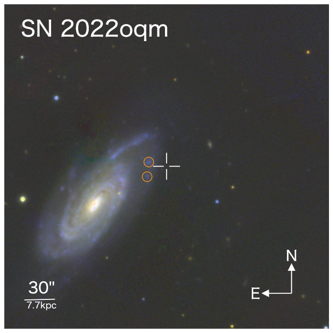
Figure 1: Pan-STARRS image the host galaxy NGC5875, at ($15^{h}09^{m}10.31^{s}$, $52^{\circ}32^{\prime}19^{\prime\prime}.72$). We indicate the location of SN  2022oqm in the white crosshairs. The closest knots of star formation (marked in orange) are $4.6$kpc and $5.3$kpc away.

SN 2022oqm was discovered in the outskirts of a face-on, spiral galaxy, NGC 5875, shown in Figure 1. Like most CaRTs, SN 2022oqm is highly offset from the center of the galaxy, located $\simeq 77.7$” (19.9 kpc) from the optical centroid of the host. The host redshift is consistent with SN 2022oqm, showing SN 2022oqm is not a chance coincidence with the galaxy’s location. SN 2022oqm is visibly offset from any ongoing star formation. To quantify the radial offset of SN 2022oqm in terms of the host light, we adopt a fractional light method previously employed in SN environmental studies (e.g., Fruchter et al., 2006; Habergham et al., 2014; Ransome et al., 2022). In the case of SN 2022oqm, we use $g$-band imaging from a Pan-STARRS PS1 pre-explosion image of the galaxy. This technique uses ellipses in the same ‘aspect ratio’ as the galaxy (position angle and axis ratio from NED with an axis ratio of $\sim$ 2.5). An ellipse that is gradually expanded until the difference between iterations becomes small (i.e. consistent with reaching the background) is the host ellipse. Another ellipse that just intercepts the SN position is the SN ellipse. The total light emitted inside the SN ellipse is divided by the total light emitted inside the host ellipse, giving the fractional light enclosed by the SN, which is $96\%$ for SN 2022oqm. Using the same method, we measure a half-life radius of 32.75” Using Pan-Starrs PS1 pre-explosion imaging of the galaxy, we find no indication of pre-explosion flux at the position of the transient, to a limiting surface brightness $24.5$ mag arcsec^-2. The two closest clusters of optical light are 18.1” (4.6 kpc) and 20.8” (5.3 kpc) away.

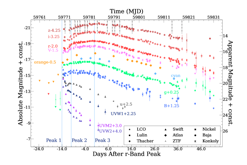
Figure 2: Multiband light curve of SN 2022oqm. Dotted vertical lines at the top represent epochs where we obtain spectroscopy. Phases of peaks 1, 2, and 3 are labeled with blue vertical lines. Upper limits ($3\sigma$) are identified as downward-facing triangles.

Photometry reveals SN 2022oqm is a multi-peaked SN. Our near-infrared to ultraviolet light curve of SN 2022oqm is shown in Figure 2. We detected an early peak that is more pronounced in shorter wavelengths at the time of detection (MJD $59771.19$). There is another, broader peak between MJD $\sim 59781$ and $\sim 59788$. We also note a weak local maximum of the $U$-band flux at MJD $59774.24$ (see Section 5.3 for a detailed discussion on the confirmation and origin of these three peaks). We note the approximate phases of these three peaks as peaks 1, 2, and 3 in Figure 2. We report phase relative to the time of maximum $r$-band flux (MJD $59784.17$) and present epochs with respect to this phase henceforth in this article. The peak luminosity of SN 2022oqm is in the typical range of peak SN Ibc luminosities ($-17$ to $-18$ mag; Drout et al. 2011), but is $\sim 1.5$ mag brighter than the population of CaRTs-Ibc at peak (De et al., 2020; Zenati et al., 2023).

In Figure 3, we show $B-V$ (top) and $r-i$ (bottom) color evolution of SN 2022oqm with known CaRTs, the well-studied SN Ib with evidence of a binary progenitor iPTF13bvn (Cao et al., 2013; Bersten et al., 2014), and a template SN Ia light curve. We use the canonical $s=1$ model from Nugent et al. (2002) to find a template SN Ia light curve (see Section 6 for a more detailed description of this model). We also show three theoretical CaRT models from Zenati et al. (2023): fca1, fca2, and fca3. The $r-i$ color evolution of SN 2022oqm matches that of other CaRTs but the $B-V$ color evolution for SN 2022oqm matches that of SNe Ia and SNe Ibc. The $B-V$ color of SN 2022oqm is bluer than that of most CaRTs. The tracks of fac1, fca2, and fca3 predict redder colors than what is seen in SN 2022oqm (see Section 7 for a detailed description of this progenitor system).

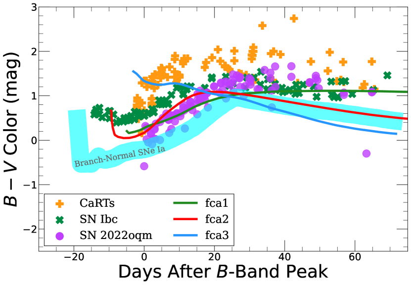
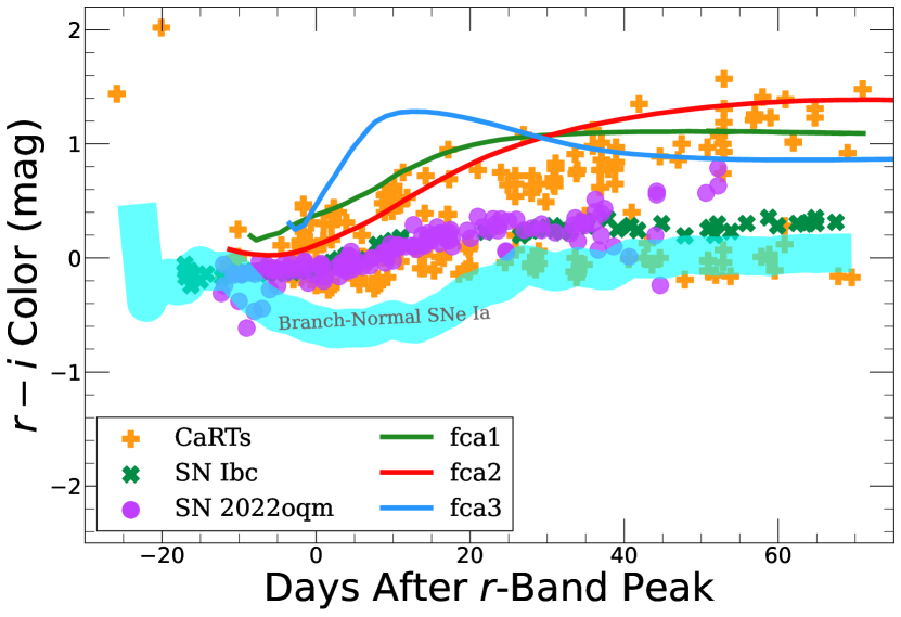
Figure 3: B-V (top) and r-i (bottom) color evolution of SN 2022oqm, compared to that of all CaRTs with well-sampled light curves, iPTF13bvn, the well-studied SN Ib with evidence of a binary progenitor, and the template of Branch-normal SNe Ia. SN 2022oqm is bluer than most CaRTs in both $r-i$ color and $B-V$ color. The three BWD models simulated by Zenati et al. (2023) are shown as $fca1$, $fca2$, and $fca3$.

3.1 Bolometric Properties

Table 2: Summary of blackbody properties of all three peaks as derived from fitting a single blackbody evolution to the SN 2022oqm light curve with extrabol. .

Parameter	Peak 1	Peak 2	Peak 3
Temperature (K)	$31,000\pm 4000$	$7,600\pm 140$	$5,800\pm 140$
Photosphere Radius (cm)	$(1.5\pm~{}0.16)\times 10^{14}$	$(9.2\pm~{}0.38)\times 10^{14}$	$(1.7\pm~{}0.1)\times 10^{15}$
Bol. Luminosity (erg/s)	$(1.5\pm~{}0.45)\times 10^{43}$	$(2.0\pm~{}0.1)\times 10^{42}$	$(2.3\pm~{}0.1)\times 10^{40}$
Bol. Magnitude	$-19.2\pm~{}0.75$	$-17.1\pm~{}0.07$	$-17.2\pm~{}0.07$

We use the extrabol (Thornton & Villar, 2022) package to estimate the bolometric luminosity ($L_{\rm bol}$), blackbody temperature ($T$), and photosphere radius ($R_{\rm phot}$) of SN 2022oqm over time. The extrabol package interpolates the light curve in each band using a Gaussian process with a 2D 3/2-Matern kernel, accounting for correlation in both time and wavelength. A blackbody spectral energy distribution (SED) is then fit to each observed epoch, inferring bolometric luminosities, blackbody radii, and blackbody temperatures with time. The fitted $L_{\rm bol}$, $T$, and $R_{\rm phot}$ are shown in Figure 4, while the bolometric luminosity, temperature, and radius during peaks 1, 2, and 3 are listed in Table 2.

At the time of detection, SN 2022oqm is very hot ($T\approx 40,000$ K) rapidly expanding and cooling between peak 1 (first detection) to peak 2, where the temperature decreases by a factor of $5$ and the bolometric luminosity decreases by a factor of $10$. After peak 2, the object continues to cool down and expand, but the bolometric luminosity increases by a factor $1.5$ until peak 3. By integrating the bolometric luminosity over all time, we find the total energy emitted $\approx 8.6\times 10^{48}$ erg. We find our derived blackbody luminosity and temperatures are within $1\sigma$ of the derived values in Irani et al. (2022).

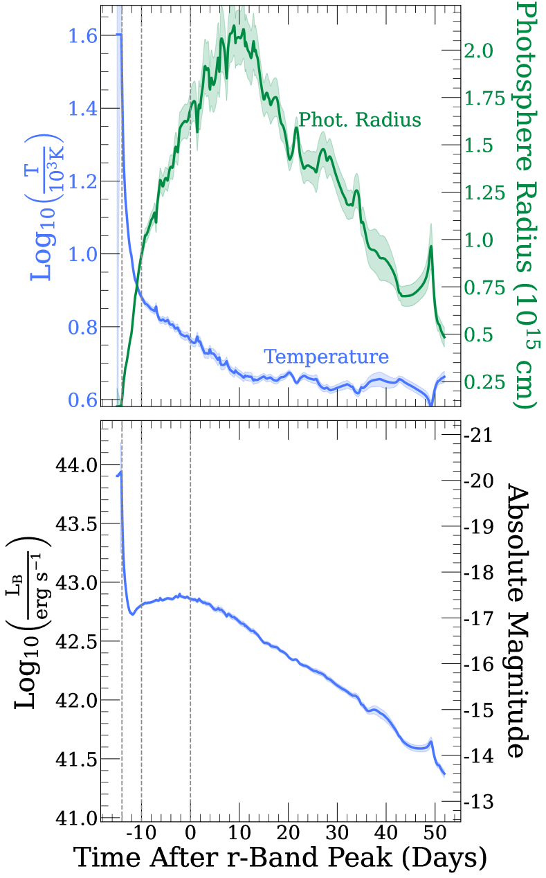
Figure 4: Blackbody fits to the photometry of SN 2022oqm, showing temperature and photosphere radius (top); and bolometric luminosity (bottom) evolution. Derived values at peaks 1, 2, and 3 are shown in grey. Numerical values are tabulated in text (see subsection 3.1).

4 Spectroscopic Analysis

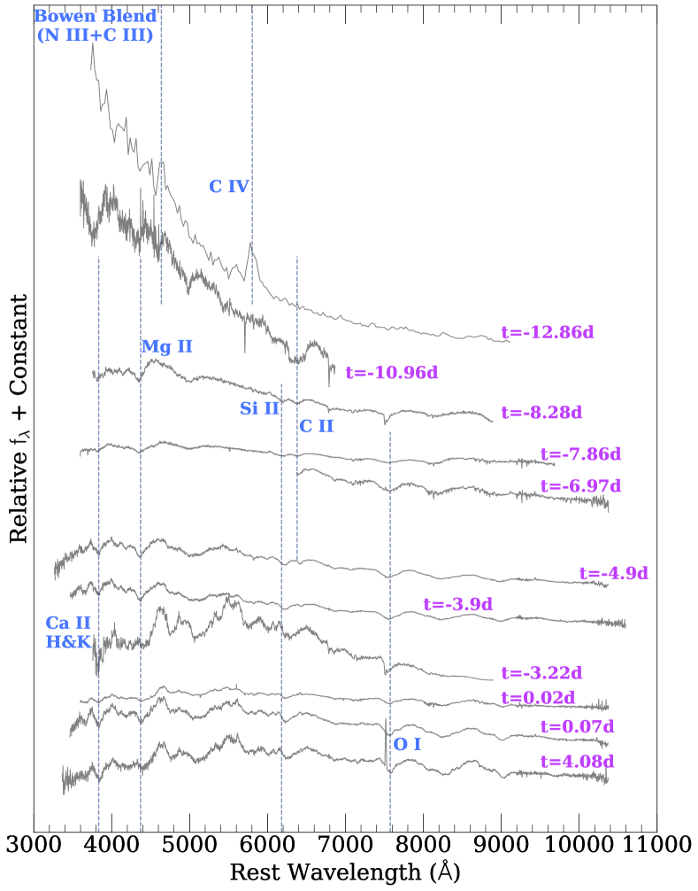
Figure 5: Spectral sequence of SN 2022oqm during $-13d\leq t\leq 5d$. We identify Ca II $\lambda\lambda 3933$ and $3968$, Mg II $\lambda 4481$, N III$\lambda 4638$, C III $\lambda 4658$, C IV $\lambda 5801$, Si II $\lambda 6347$, C II $\lambda 6580$, and O I $\lambda 7775$ with blue vertical lines. All spectra are in the rest frame. The vertical axis is scaled linearly.

We present 19 spectra that were taken between $t=-14$d and $t=62$d in figures 5, 6, and 7. The earliest spectrum ($-14$d) is dominated by a blue continuum with a C IV emission feature at $5805~{}\mathrm{\AA}$ and N III at $4638~{}\mathrm{\AA}$. Irani et al. (2022) presents multiple spectra with a higher signal-to-noise ratio at this phase, identifying the same emission features in addition to strong O III, O IV, and O V features. The presence of such high ionization levels suggests the presence of an intense UV radiation field (Leloudas et al., 2019; Quimby et al., 2007). Indeed fitting a blackbody curve to the earliest spectrum suggests a temperature in excess of $3\times 10^{4}$ K, in agreement with our photometrically inferred earliest temperature (see Figure 4). The very high temperature points to the presence of shock cooling during this phase caused by the SN blastwave interacting with the surrounding circumstellar material (CSM). The earliest spectrum suggests that the CSM lacks H and He, although C and O are observed.

We observe the Ca II H&K complex at $3933~{}\mathrm{\AA}$, the Mg II $\lambda 4481$ feature, a weak S II $\lambda 6355$ absorption line, a weak C II $\lambda 6580$ absorption line, and an O I $\lambda 7775$ feature before peak 3. The NIR spectrum taken on $t=-6$d (Fig 7) shows no clear evidence of helium, unlike many CaRTs (see section 6 for a detailed comparison between SN 2022oqm and CaRT spectroscopic signatures).

By $t\approx 30d$, we find the SN has begun transitioning to its nebular phase, revealing significant forbidden line emission. By this time, a clear [Ca II] emission feature at $7300~{}\mathrm{\AA}$ becomes apparent, confirming that this SN is a CaRT. Using the most recently available spectrum ($t=62d$), in which SN 2022oqm approaches the nebular phase, we attempt to measure an emission flux ratio [Ca II] $\lambda$7324/[O I] $\lambda$6300. Because [O I] emission is not clearly detected, we measure the total flux within the equivalent width of the [Ca $\lambda$7324] line centered at the [O I] $\lambda\lambda$6300, 6364 line location. We place a lower limit of $\approx 4.4$, greater than the defined cutoff of $2$ to be considered a CaRT (Perets et al., 2010; Jacobson-Galán et al., 2022; De et al., 2020).

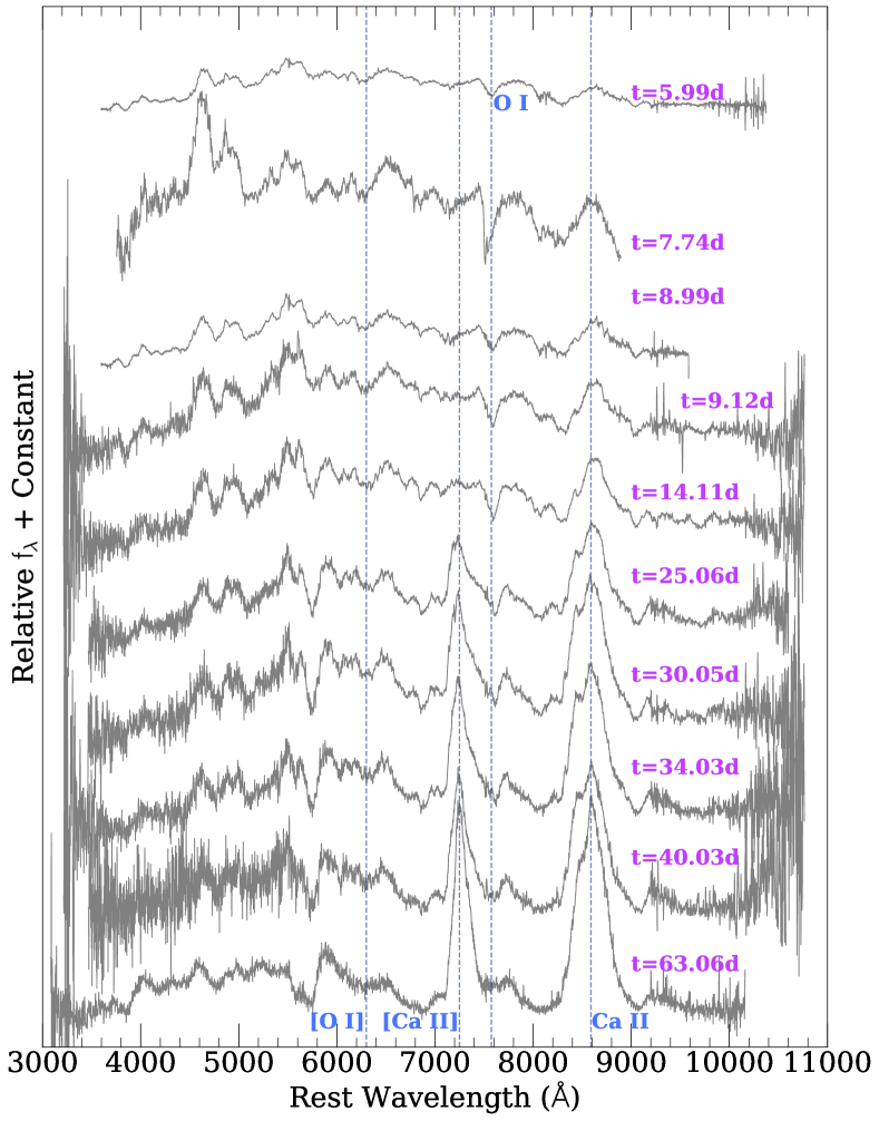
Figure 6: Spectral sequence of SN 2022oqm during $5d\leq t\leq 65d$. The features O I $\lambda 7775$, [Ca II] $\lambda 7300$, and Ca II $\lambda\lambda 8498$, $8542$, and $8662~{}\mathrm{\AA}$ are clearly detected and marked. We also show the location of [O I] $\lambda 6300$, but this line is not clearly detected in our spectral sequence. The strong [Ca II] $\lambda 7300$ feature is characteristic of CaRTs. The Ca complex found redward of $8000~{}\mathrm{\AA}$ is a permitted feature and is not used to qualify a transient as a CaRT. All spectra are in the rest frame. The vertical axis is scaled linearly.

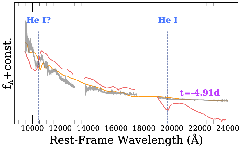
Figure 7: NIR Spectrum of SN 2022oqm taken at $t=-4.9$d in grey. Also overlaid are the corresponding phase TARDIS radiative transfer simulation (see Figure 10) in orange and the NIR spectrum of the SN Ib SN 2008D in red. In contrast to SN 2022oqm, SN 2008D has clear He I $\lambda 10830$ and He I $\lambda 20581$ absorption features. The vertical axis is scaled linearly.

Spectroscopic observations enable a census of elemental abundance, density, and velocity structures within the SN ejecta. As the ejecta expand, optical depth decreases with time, and the photosphere recedes into deeper layers of the ejecta. By measuring the line velocity of several elements over time, one can probe the velocity gradient of the ejecta. We present the velocities of O I$\lambda 7775$, Si II $\lambda 6355$, and Ca II H&K absorption lines during the photospheric phase of the SN in Figure 8. O I$\lambda 7775$ velocity is roughly constant at $\sim 8000$ km s^-1 during the $\sim 20$ days when this line is visible. Si II$\lambda 6355$ declines in velocity, starting from $\sim 5000$ km s^-1 and reaching $3000$ km s^-1. At early times, we observe Ca II H&K at $\sim 15000$ km s^-1, which remains constant with the O I$\lambda 7775$ velocity from the time of peak 2 until immediately after peak 3. The times of peaks 1, 2, and 3 are highlighted with grey vertical lines. These velocities are typical for CaRTs and SNe Ic (mod, 2016; De et al., 2020).

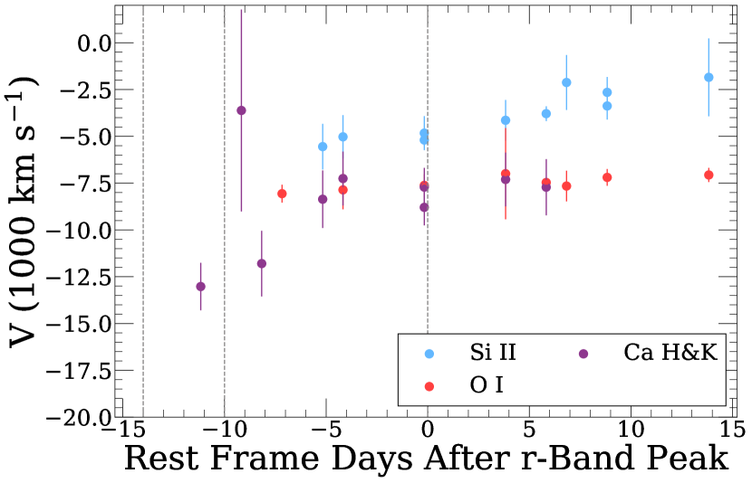
Figure 8: Velocities of the Si II, O I, and Ca H&K absorption lines measured during the photospheric phase. Silicon is consistently at a smaller velocity (and therefore radius) than oxygen and calcium, which seem to be at similar radius throughout the early evolution. Times of peaks 1, 2, and 3 are shown as dotted grey lines.

4.1 Spectral synthesis analysis

We model the observed spectral series of SN 2022oqm using TARDIS (Kerzendorf & Sim, 2014), a one-dimensional Monte-Carlo radiative transfer code that numerically solves the radiative transport equation and models the spectral emission of SN ejecta. TARDIS treats photon-atom line interactions using a macroatom formalism, where the “macroatom” is the combination of the photon and atom. The macroatom formalism gives how the excited atom eventually de-excites and emits a photon and is explained in detail by Lucy (2002). TARDIS also assumes local thermodynamic equilibrium to simplify modeling the photon-atom interactions. In order to model helium, we have used the recomb-nlte treatment, which considers He I excited states as if they are in local thermodynamic equilibrium with higher ionization He II (see e.g. Boyle et al., 2017).

By assuming homologous expansion of ejecta, TARDIS can parameterize ejecta layers by velocity. TARDIS takes ejecta density distribution, elemental abundance distribution, bolometric luminosity, and time since explosion as input to simulate an instantaneous SN spectrum produced by a prescribed range of velocities within the ejecta.

The CO21 model (Iwamoto et al., 1994) and the W7 Branch model (Nomoto et al., 1984; Branch et al., 1985) are the canonical density profiles in TARDIS for stripped-envelope and thermonuclear explosions respectively. We find that neither of these models reproduces the SN 2022oqm spectra well. As such, we utilize an exponential ejecta density profile to adequately fit the spectral sequence of SN 2022oqm. These three density profiles are reproduced in Figure 9. The exponential density profile mimics the Ic-like outer ejecta profile throughout the ejecta. The exponential density profile is constructed as $\rho\propto\exp\left(\frac{-3v}{10^{4}~{}\rm{km~{}s^{-1}}}\right)$ and has an integrated mass of $M_{ej}=0.57$ M_⊙. The agreement to an exponential density profile is reminiscent of a disk-like ejecta structure (i.e. an alpha-disk model), but here we are limited to a one-dimensional geometry and therefore do not truly probe the angular distribution of the ejecta.

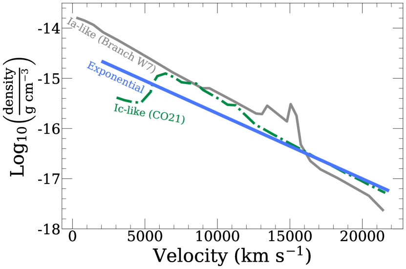
Figure 9: We use the exponential ejecta mass density profile to model SN 2022oqm ejecta using TARDIS. This is shown in relation to two commonly used density profiles for SN Ia and SN Ic modeling. The exponential density profile, which is shallower than both the Ia-like and Ic-like profiles, provides the best fit to the SN 2022oqm ejecta spectra. The fitted spectra are shown in Figure 10

We fit four optical spectra at $t=-7.86,-3.22,0.07,4.08$ d and one NIR spectrum at $t=-4.9$ d. Each simulation fits the velocity range and abundance of He, C, O, Ne, Si, Ca, and Fe-peak elements (including Ni and Co). We present atomic abundances which are denegerate in our modeling in the same category (e.g. Ne and O as “Ne+O” and Ni and Co as “Ni+Co”). We assume these elements are uniformly distributed through the velocity range fitted by each spectral fit. We show the fitted spectra in Figure 10 and the abundance distributions for each element in Figure 11. We find a general agreement between the simulated and the observed spectra, where the majority of spectral features are well reproduced. Some specific features, such as the broad absorption around $5200~{}\mathrm{\AA}$ at peak 3 are not correctly reproduced, likely due to a different ionization level of the line responsible for that absorption. We find a total ejecta mass of $\sim 0.6~{}M_{\rm{\sun}}$.

The resulting abundance pattern is characterized by: 1) a predominant ejecta composition with a homogeneous distribution of both light elements (He, C, O, and Ne) and Fe-peak elements (Fe, Co, and Ni); and 2) a low Ca abundance at velocities $v_{ej}\gtrsim 7900$ km s^-1, rapidly increasing when the most inner regions of the ejecta become visible at late epochs, e.g. days after peak brightness. The roughly uniform distribution of both Fe-peak and Ni+Co abundances throughout the ejecta shows agreement with the $\rm{{}^{56}Ni}$ mixing and double-decay model suggested in subsections 5.4. A more detailed analysis of the iron features in the spectra could elucidate this, but such analysis is beyond the scope of this article. The enhancement of Ca during later spectra is consistent with the broadening of the later Ca lines observed $\sim$30 days after peak. A lack of distinct O and Ne features in our optical spectra mean that we are unable to constrain the individual abundance of either O or Ne.

Detailed spectroscopic modeling suggests a low He abundance in the ejecta of SN 2022oqm. Through TARDIS modeling, we find a helium mass upper limit of $8.43\times 10^{-3}~{}M_{\mathrm{\sun}}$, corresponding to a mass fraction of $\sim 1.5\%$ (see Figure 11). In addition, the commonly used He I $\lambda 10830$ and He I $\lambda 20581$ features are nonexistent in the NIR spectrum of SN 2022oqm (see Figure 7). A dubious absorption feature is present near the He I $\lambda 10830$ line, but this is likely a blend of other elements, as it cannot be properly captured by modeling using TARDIS, and because the velocity of such He would need to be $\gtrapprox 2\times 10^{4}$ km s^-1, a velocity that is inconsistent with other measures of velocity (see Figure 8).

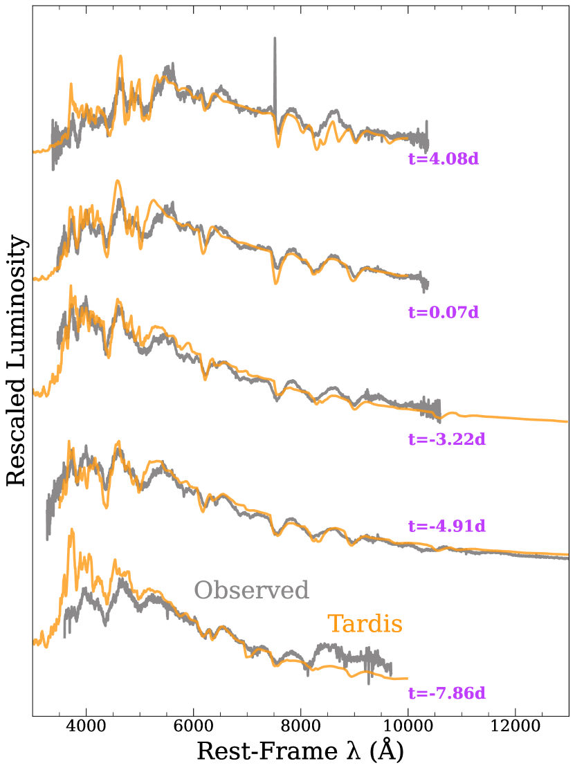
Figure 10: Spectral series of SN 2022oqm (grey curves) and the corresponding TARDIS radiative transfer simulation (orange curves). We find good agreement between the TARDIS models and our observed spectral sequence. The vertical axis is scaled linearly. The inferred ejecta density profile and the ejecta abundances, as inferred from TARDIS are shown in Figures 9 and 11, respectively.

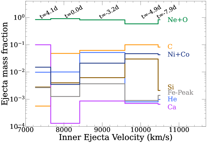
Figure 11: The abundance pattern derived from TARDIS fitting to spectra at $t=-7.86,-3.22,0.07,4.08$ d. Atomic abundances which are degenerate via TARDIS modeling are combined into one category (i.e. Ne+O, Ni+Co, and Fe-Peak, which is Fe, Ti, and Cr). The distributions of Fe-peak elements, radioactive elements, and lower-mass elements are flat throughout the ejecta.

4.2 Comparing SN 2022oqm to Other Transients

We overlay the spectrum of SN 2022oqm with those of SN 2007gr (a SN Ic, Hunter et al. 2009; Valenti et al. 2008), SN 2021gno (a CaRT, Jacobson-Galán et al. 2022), and SN 2012Z (a SN Iax, Stritzinger et al. 2015; McCully et al. 2022) at peak (Figure 12) and during their nebular phases (Figure 13). At peak, we show Ca II $\lambda\lambda 3933$ and $3968$, Si II $\lambda 6347$, and O I $\lambda 7775$ with vertical lines, while for the nebular phase (Fig. 13), we show the [O I] $\lambda 6300$, [Ca II] $\lambda 7300$, and Ca II $\lambda\lambda 8498$, $8542$, and $8662$ with vertical lines. During the photospheric phase of SN 2022oqm, the spectrum closely resembles that of a SN Ic, where the strengths of calcium, silicon, and oxygen appear to be almost identical. The only inconsistency appears to be at shorter wavelengths, where iron blanketing reduces flux more strongly in CaRTs than in SNe Ic. We also note that helium is clearly detected in at least some CaRTs but not in SN 2022oqm or the SN Ic. In the nebular phase, however, SN 2022oqm has a very different spectrum from that of the SN Ic. During the nebular phase, SNe Ic spectra feature a strong [O I] $\lambda 6300$ emission line (Gaskell et al., 1986; Shivvers et al., 2019). This line is not detected in the spectrum of SN 2022oqm, which instead has a very strong [Ca II] $\lambda 7300$ emission line, characteristic of CaRTs.

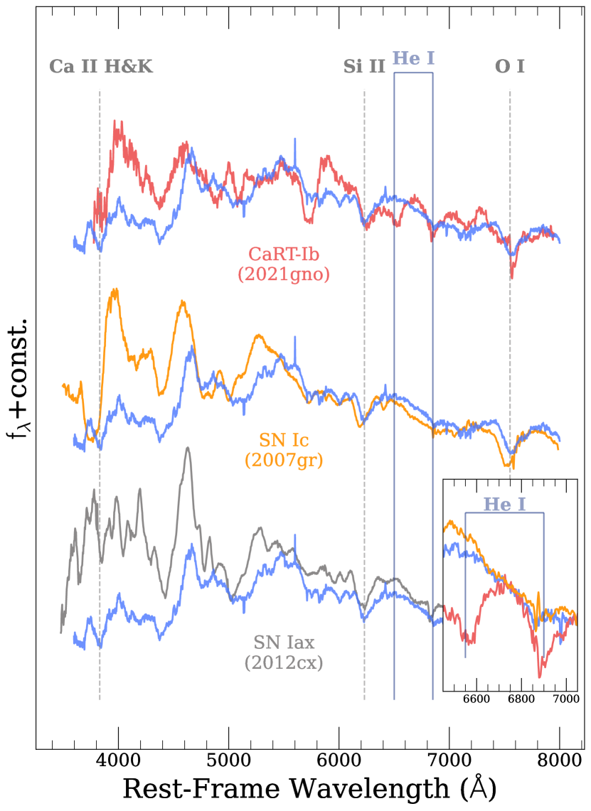
Figure 12: Peak-time spectrum of SN 2022oqm (blue) overlaid with peak-time spectra of SN 2012Z (SN Iax), SN 2007gr (SN Ic), and SN 2021gno (CaRT). Absorption lines visible in the spectrum of SN 2022oqm are marked. SN 2022oqm appears quite similar to SN Iax, SN Ic, and the CaRT. We show Ca II $\lambda 3933~{}\mathrm{\AA}$, Si II $\lambda 6347$, He I $\lambda 6678$, He I $\lambda 7065$, and O I $\lambda 7775$, where the helium lines are only clearly discernable in the CaRT-Ib spectrum.

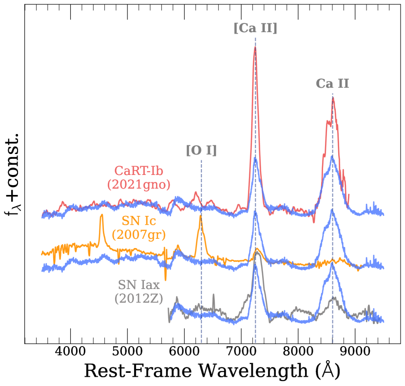
Figure 13: Nebular spectrum of SN 2022oqm overlaid with nebular spectra of SN 2012Z (SN Iax), SN 2007gr (SN Ic), and SN 2021gno (CaRT). The [Ca II] forbidden emission line at $7300~{}\mathrm{\AA}$ is present in all spectra but is strongest in the CaRTs. The [O I] forbidden emission at $6300~{}\mathrm{\AA}$ is completely absent in the spectrum of SN 2022oqm. Note that this [O I] line is stronger in the SN Ic, a characteristic difference between SNe Ic and Ca-Ic.

5 Detailed Light Curve Modeling

Table 3: Best-fit parameters of each model produced in MOSFiT . The goodness of fit is parameterized by the Watanabe Akaike Information Criterion (WAIC) measure and by the reduced chi-squared ($\chi^{2}_{\mathrm{red}}$) measure.

Module	Parameter	Power Law + Single $\mathrm{{}^{56}Ni}$ Decay (Section  5.1)	Single $\mathrm{{}^{56}Ni}$ Decay (Section 5.2)	Double $\mathrm{{}^{56}Ni}$ Decay (Section 5.2)	Power Law + Double $\mathrm{{}^{56}Ni}$ Decay (Section 5.3)
Power Law	$log~{}\frac{L_{\mathrm{pow}}}{\mathrm{erg~{}s^{-1}}}$	$43.43^{0.89}_{1.17}$	–	–	$42.73^{2.04}_{1.93}$
	$\alpha$	$1.05^{0.02}_{0.02}$	–	–	$4.30^{0.48}_{0.42}$
	$log~{}\frac{t_{\mathrm{pow}}}{\mathrm{days}}$	$-0.5^{1.11}_{0.83}$	–	–	$0.20^{0.45}_{0.46}$
	$log~{}\frac{v_{\mathrm{ej,pow}}}{\mathrm{km~{}s^{-1}}}$	$4.14^{0.03}_{0.05}$	–	–	$4.10^{0.05}_{0.04}$
	$\kappa_{\mathrm{pow}}$	$0.1^{0.05}_{0.03}$	–	–	$0.13^{0.04}_{0.05}$
	$log~{}\frac{T_{\mathrm{pow}}}{\mathrm{K}}$	$3.79^{0.01}_{0.01}$	–	–	$3.99^{0.07}_{0.36}$
$\mathrm{{}^{56}Ni}$ Decay 1	$log~{}\frac{m_{\mathrm{1,ej}}}{\mathrm{M_{\odot}}}$	$-0.24^{0.03}_{0.05}$	$-0.26^{0.02}_{0.02}$	$-0.07^{0.19}_{0.22}$	$-0.13^{0.18}_{0.11}$
	$log~{}f_{\mathrm{1,Ni}}$	$-0.89^{0.05}_{0.03}$	$-0.79^{0.03}_{0.02}$	$-1.19^{0.14}_{0.19}$	$-1.15^{0.10}_{0.17}$
	$M_{\mathrm{1,Ni}}$	$0.074_{0.001}^{0.001}$	$0.09_{0.002}^{0.003}$	$0.055_{0.002}^{0.002}$	$0.05_{0.002}^{0.002}$
	$log~{}\frac{v_{\mathrm{1,ej}}}{\mathrm{km~{}s^{-1}}}$	$3.99^{0.01}_{0.01}$	$4.31^{0.01}_{0.01}$	$3.96^{0.02}_{0.02}$	$3.95^{0.01}_{0.01}$
	$log~{}\frac{T_{\mathrm{1}}}{\mathrm{K}}$	$2.7^{0.39}_{0.42}$	$3.68^{0.01}_{0.0}$	$2.68^{0.43}_{0.42}$	$2.72^{0.37}_{0.40}$
	$log~{}\kappa_{\mathrm{\gamma,12}}$	$-0.99^{0.02}_{0.01}$	$-0.99^{0.02}_{0.01}$	$-0.18^{0.21}_{0.22}$	$-0.43^{0.14}_{0.17}$
	$\kappa_{\mathrm{1,2}}$	$0.19^{0.0}_{0.01}$	$0.19^{0.0}_{0.01}$	$0.12^{0.05}_{0.04}$	$0.14^{0.04}_{0.05}$
	$\log~{}\frac{t_{\mathrm{d}}}{\mathrm{days}}$	$1.09^{0.08}_{0.9}$	$0.78_{0.01}^{0.01}$	$1.1_{0.02}^{0.02}$	$1.04_{0.02}^{0.02}$
$\mathrm{{}^{56}Ni}$ Decay 2	$log~{}\frac{m_{\mathrm{2,ej}}}{\mathrm{M_{\odot}}}$	–	–	$-1.01^{0.2}_{0.16}$	$-0.87^{0.16}_{0.12}$
	$log~{}f_{\mathrm{2,Ni}}$	–	–	$-0.43^{0.15}_{0.19}$	$-0.55^{0.11}_{0.16}$
	$M_{\mathrm{2,Ni}}$	–	–	$0.04_{0.002}^{0.002}$	$0.04_{0.002}^{0.002}$
	$log~{}\frac{v_{\mathrm{2,ej}}}{\mathrm{km~{}s^{-1}}}$	–	–	$4.3^{0.04}_{0.04}$	$4.22^{0.02}_{0.02}$
	$log~{}\frac{T_{\mathrm{2}}}{\mathrm{K}}$	–	–	$3.78^{0.01}_{0.01}$	$3.78^{0.01}_{0.01}$
	$log~{}\kappa_{\mathrm{\gamma,12}}$	–	–	$-0.18^{0.21}_{0.22}$	$-0.43^{0.14}_{0.17}$
	$\kappa_{\mathrm{1,2}}$	–	–	$0.12^{0.05}_{0.04}$	$0.14^{0.04}_{0.05}$
	$\log~{}\frac{t_{\mathrm{d}}}{\mathrm{days}}$	–	–	$0.46_{0.06}^{0.06}$	$0.57_{0.04}^{0.04}$
General	$log~{}\sigma$	$-0.63^{0.01}_{0.01}$	$-0.43^{0.04}_{0.02}$	$-0.65^{0.01}_{0.01}$	$-0.69^{0.01}_{0.01}$
	WAIC	660.4	550.4	727.1	758.1
	$\chi^{2}_{\mathrm{red}}$	1.41	3.53	1.52	1.04

In this section, we model the light curve of SN 2022oqm using several potential underlying power sources through the Modular Open-source Fitter for Transients (MOSFiT, Guillochon et al. 2018). MOSFiT is an open-source software which self-consistently models the time-variable SED following the framework originally presented in Arnett (1982). For each fit, we present goodness of fit through the Watanabe-Akaike Information Criterion (WAIC) score, where a higher score represents a better fit to the data. The WAIC score accounts for parameter size by punishing models with more parameters. Therefore, the WAIC score presents a method of comparing models with different parameter numbers and avoids the problem of overfitting. A WAIC score increase of at least $10$ implies a significantly better model fit (Watanabe, 2013; Gelman et al., 2014). We also measure goodness of fit for each model with the reduced chi-squared ($\chi^{2}_{\mathrm{red}}$) term.

The early excess in the light curve seen in peak 1 (see Figure 2) is reminiscent of shock cooling following breakout of a SN shockwave out of surrounding circumstellar material (CSM, see e.g, Smith 2017; Piro et al. 2021). Following this peak, the behavior of the SN near peak 3 is similar to the more classical SN light curve, which is powered by the radioactive decay of $\rm{{}^{56}Ni}$ diffused through optically thick ejecta (Arnett, 1982; Chatzopoulos et al., 2012). Within this framework, the ejecta mass ($m_{\mathrm{ej}}$), ejecta velocity ($v_{\mathrm{ej}}$), and greybody opacity ($\kappa$) are fully degenerate, as all three primarily impact the overall diffusion timescale of the transient: $t_{d}\propto\sqrt{\kappa m_{\mathrm{ej}}/v_{\mathrm{ej}}}$. As such, we present $t_{d}$ in addition to these three parameters.

5.1 Joint Shock Breakout and Radioactive Decay Model

First, we explore a toy model in which the emission can be modeled by the combination of a power-law model (a reasonable description for shock cooling) and a radioactive decay model. The first peak would be captured by the power-law model and the subsequent light curve evolution would be captured by the radioactive decay. For the power law model, we utilize a power-law source of bolometric luminosity, described by:

$$L_{1}=L_{\rm pow}{\left(t/t_{\rm pow}\right)}^{-\alpha},$$ (1)

where $L_{\rm pow}$ is a luminosity scaling factor, $t_{\rm pow}$ is the time-scale of decay, and $\alpha$ is the power-law index. This emission is treated as a single blackbody, with a characteristic photosphere velocity $v_{\rm ej,pow}$, opacity $\kappa_{\rm pow}$, and minimum photosphere temperature $T_{\rm pow}$ (see Villar et al. 2017; Guillochon et al. 2018 for more details).

We note that the power-law model is a well-known model to describe the luminosity of shock-heating material over time (see e.g., Nakar & Sari 2010; Piro et al. 2021). In this case, the time-dependence is directly linked to the outer ejecta profile, $L_{1}\propto t^{-4/(n-2)}$, where $n$ is the index of the power law that describes the outer ejecta density profile. We also note that we do not allow for photons emitted via this power-law model to diffuse through any material after emission. This is equivalent to assuming there is no material beyond the region where these power-law photons are emitted which can diffuse photons. Allowing diffusion of the power-law photons results in a much poorer fit (see Appendix B, where we attempt this fit).

The radioactive decay of ⁵⁶Ni produces gamma-rays that are thermalized in optically thick ejecta, which then emit as a blackbody, driving peaks 2 and 3 (Arnett, 1982; Chatzopoulos et al., 2012; Villar et al., 2017). The free parameters corresponding to this are the $\mathrm{{}^{56}Ni}$ mass ($m_{\mathrm{Ni}}$) and diffusion time $t_{d}\propto\sqrt{\kappa m_{\mathrm{ej}}/v_{\mathrm{ej}}}$ (see Power Law + Single $\mathrm{{}^{56}Ni}$ Decay column in Table 3).

We present the fitted light curve in Figure 14, and show the fitted parameters in Table 3. We overall find agreement between the model and data ($\chi^{2}_{\mathrm{red}}=1.41$), but the fit is poor in the $U$, $UVW1$, and $UVM2$ bands. Most notably, this model overpredicts the emission in $UVM2$ by $\sim 1$ mag after peak 1.

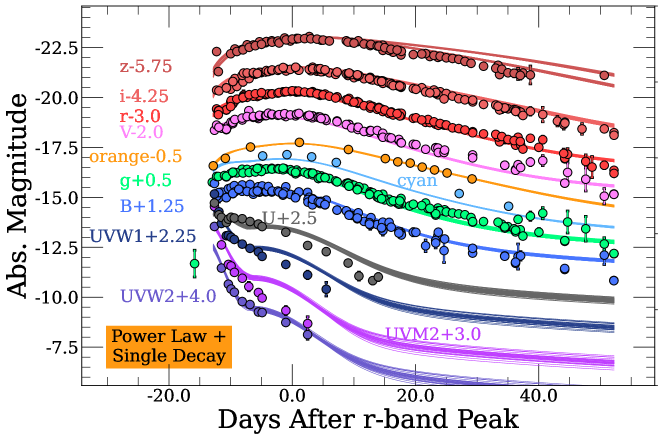
Figure 14: Best-fit model to the UVONIR light curves for the shock cooling-$\mathrm{{}^{56}Ni}$ model. Points represent observed photometry, while colored lines are random draws from the resulting posterior. Fitting is done using the MOSFiT package.

5.2 Capturing Individual Peaks with Radioactive Decay Models

To find a better fit than was shown in Subsection 5.1, we focus on only peak 3. We cut peaks 1 and 2 from the light curve by including only data points from $t>-6$ d and fit a single radioactive decay model. We find an ejecta mass of $0.55~{}\mathrm{M_{\odot}}$, with a ${}^{56}\rm{Ni}$ fraction $f_{\rm Ni}\approx 0.16$, corresponding to ${}^{56}\rm{Ni}$ mass $m_{\rm Ni}=0.09~{}\mathrm{M_{\odot}}$. Even though the first two peaks have been removed for this fit, the best fit still requires all $0.09~{}M_{\sun}$ to power peak 3, hinting that a single radioactive decay model of ${}^{56}\mathrm{Ni}$ does not fully account for the photons emitted during peak 3.

We attempt to fit peaks 2 and 3 with a toy “two-zone” model, by considering two discrete ${}^{56}\rm{Ni}$ central sources. This is similar to Maeda et al. 2003, who presented a similar formalism of a two-zone model by constructing two concentric sources of photons. Photons emitted by ${}^{56}\rm{Ni}$ located at larger radii diffuse through a total mass $m_{2,\mathrm{ej}}$, before escaping from the system and driving peak 2. Photons emitted from the ${}^{56}\rm{Ni}$ decay that are located deeper inside the ejecta would diffuse through a larger amount of mass ($m_{1,\mathrm{ej}}+m_{2,\mathrm{ej}}$) before escaping, resulting in the delayed, third peak.

We create a custom model in MOSFiT to perform this fit. We find an inner ejecta layer with mass of $log_{10}~{}[m_{1,\mathrm{ej}}/\mathrm{M_{\sun}}]=-0.07^{0.19}_{0.22}$ and a ${}^{56}\rm{Ni}$ fraction of $log_{10}~{}f_{\rm 1,Ni}=-1.19^{0.14}_{0.19}$, corresponding to $log_{10}~{}[M_{1,\mathrm{Ni}}/\mathrm{M_{\sun}}]=0.055^{0.002}_{0.002}$ of ${}^{56}\rm{Ni}$. We find an outer ejecta layer with mass of $log_{10}~{}[m_{2,\mathrm{ej}}/\mathrm{M_{\sun}}]=-1.01^{0.20}_{0.16}$ and a ${}^{56}\rm{Ni}$ fraction of $log_{10}~{}f_{\rm 2,Ni}=-0.43^{0.15}_{0.19}$, corresponding to $log_{10}~{}[M_{2,\mathrm{Ni}}/\mathrm{M_{\sun}}]=0.04^{0.002}_{0.002}$ of ${}^{56}\rm{Ni}$.

5.3 Joint Shock Breakout and Double Radioactive Decay Model

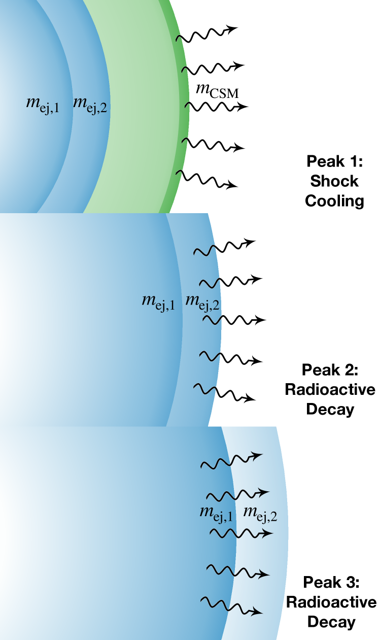
Figure 15: Schematic to highlight the sources of photons during peaks 1, 2, and 3 in our shock cooling-double decay model (Section 5.3). Fits to this model are shown in Figure 16 and the fitted parameters are shown in the far-right column of Table 3.

Finally, we combine the power-law model of peak 1 to the Double ${}^{56}\rm{Ni}$ Decay model of peaks 2 and 3 to fit the entire light curve. In such a model, peak 1 is powered by shock cooling of the CSM following shock breakout. Peak 2 is powered by radioactive decay of ${}^{56}\rm{Ni}$ distributed near the outer regions of the ejecta. Peak 3 is powered by radioactive decay of ${}^{56}\rm{Ni}$ distributed near the inner regions of the ejecta. Photons emitted from the inner regions of the ejecta diffuse through more mass and take longer before they are emitted. We show a schematic of this model in Figure 15. We find a power-law index of $\alpha=4.3^{0.48}_{0.42}$, $log_{10}~{}[L_{pow}/\mathrm{erg~{}s^{-1}}]=42.73^{2.04}_{1.93}$, $log~{}[t_{pow}/\mathrm{days}]=0.2^{0.45}_{0.46}$ days. The inner layer of ejecta has $log_{10}~{}[m_{1,\mathrm{ej}}/\mathrm{M_{\sun}}]=-0.13^{0.18}_{0.11}$ and ${}^{56}\rm{Ni}$ mass of $m_{1,\mathrm{Ni}}=0.05^{0.002}_{0.002}~{}\mathrm{M_{\odot}}$. The outer layer of ejecta has $log_{10}~{}[m_{2,\mathrm{ej}}/\mathrm{M_{\sun}}]=-0.87^{0.16}_{0.12}$ and ${}^{56}\rm{Ni}$ mass of $m_{Ni,2}=0.04^{0.002}_{0.002}~{}\mathrm{M_{\odot}}$. The total ejecta mass from this model is $\log\left[(m_{1}+m_{2})/M_{\sun}\right]=-0.06\pm 0.20$, and $m_{1,\mathrm{Ni}}+m_{2,\mathrm{Ni}}\approx 0.09~{}\mathrm{M_{\odot}}$ of it is ${}^{56}\rm{Ni}$.

Compared to the model presented in Subsection 5.1, our joint Power Law + Double $\rm{{}^{56}Ni}$ decay provides a better fit to the SN 2022oqm photometry. We obtain a WAIC score of 758 and reduced $\chi^{2}_{\mathrm{red}}\approx 1$. This suggests that the SN 2022oqm light curve is powered by three distinct sources, leading to the triple peaked behavior seen in Figure 2.

We note here that all three peaks are not clearly visible in all bands. Rather, peak 1 is most clearly visible in UV bands, e.g., Swift; peaks 1 and 2 are visible in slightly longer wavelengths, e.g., $u$-band; and peak 3 is strongest in longer wavelengths, e.g., $r$-band. To clearly visualize these peaks, we overlay the data in these bands with our MOSFiT models in these three regimes in the right panel of Figure 16.

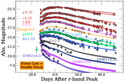
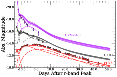
Figure 16: Left: The result of fitting shock cooling and the double Arnett model to the photometry of peaks 1, 2, and 3. In agreement with the double Arnett model, this fit finds a total ${}^{56}\rm{Ni}$ mass of $\sim 0.09~{}\mathrm{M_{\odot}}$, with total ejecta mass $\sim\mathrm{M_{\odot}}$. Right: Contribution to r-, U-, and UVM2-band light curves from the three sources of photons. Peak 1 is powered by shock interactions with CSM, and is most clearly visible in UV bands. Peak 2 is powered by the radioactive decay of ${}^{56}\rm{Ni}$ in the outer ejecta, and is most clearly visible in the U-band. Because photons emitted by this overdensity of ${}^{56}\rm{Ni}$ have less mass to diffuse through, they will be observed before photons emitted by ${}^{56}\rm{Ni}$ in more inner regions of the ejecta. Peak 3, which is most clear in the r-band, is powered by the radioactive decay of ${}^{56}\rm{Ni}$ in the inner ejecta. Fitting is done using the MOSFiT package.

5.4 Reflections on Photometric Modeling

Through Sections 5.1, 5.2, and 5.3, we find that

1. Peaks 2 and 3 can be modeled as two distinct radioactive peaks

2. The total nickel mass is $\sim 0.09~{}\mathrm{M_{\odot}}$

3. Peak 1 can be modeled with a power-law model of emission in time, suggesting a shock cooling peak

The presence of narrow, highly ionized emission lines in the earliest spectrum also suggests emission from shocked material during the first $\sim 2$ d of this SN (see Section 4). From Section 5.3, we find total ejecta mass ($0.56~{}M_{\odot}\leq m_{\rm 1,ej}+m_{\rm 2,ej}\leq 1.4~{}M_{\odot}$) is within $1\sigma$ of the mass found by spectroscopic modeling ($\approx 0.6~{}M_{\sun}$, see Section 4), lending further support to the ${}^{56}\rm{Ni}$ decay model during peaks 2 and 3.

We emphasize that our double $\mathrm{{}^{56}Ni}$ decay model is a toy approximation for a multi-zone model. Our model suggests that the light curve is powered by a centrally located radioactive material, with a small fraction of Fe-peak elements mixed into the outer ejecta layers. In particular, the fact that the best fit model requires that at least some radioactive material is not centrally located hints at the mixing of ${}^{56}\rm{Ni}$ throughout the ejecta. The mixed distribution of ${}^{56}\rm{Ni}$ throughout the ejecta is consistent with our spectroscopic modeling (see Figure 11). The outer ejecta layer is less massive, more nickel-rich, and faster moving than the inner ejecta layer. In addition, such agreement with such a two-zone model of SN emission highlights the need for more robust multidimensional analytical models of SNe emission (Maeda et al., 2003).

6 Comparing to the CaRT Population

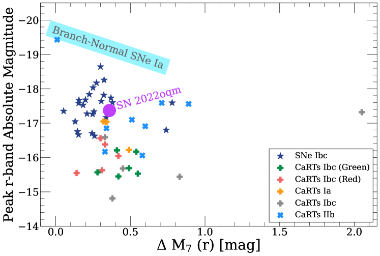
Figure 17: Comparison of the decline rate and absolute magnitude for CaRTs, SNe Ibc, and SNe Ia. These SNe Ibc are presented in Drout et al. (2011). We generate the sample of Branch-Normal SNe Ia using the methodology described in Equations 2 and 3.CaRTs Ia, green CaRTs Ibc, and red CaRTs Ibc are presented in De et al. (2020). SN 2022oqm is among the brightest CaRTs detected. Its peak $r$-band absolute Magnitude is typical of SNe Ibc. CaRTs Ibc shown as gray pluses are unclassified as Green or Red either because the De et al. (2020) sample pre-dates their discovery or because De et al. (2020) did not classify them as Green or Red. These are SN 2007Ke(Chu et al., 2007; Perets et al., 2010), PTF11bij (Kasliwal et al., 2012), SN 2019bkc (Prentice et al., 2020; Zheng & Yu, 2021), SN 2021gno (Jacobson-Galán et al., 2022), and SN 2021inl (Jacobson-Galán et al., 2022). The sample of CaRTs IIb is presented in Das et al. (2022).

SN 2022oqm is the 40th transient spectroscopically classified as a CaRT. We present an aggregate list of all known CaRTs at the time of writing in Table 5, along with the original references and basic observational properties. Although the prototypical CaRT is SN 2005E (Perets et al., 2010), several CaRTs were detected before 2005 (see Table 5). The most comprehensive study of CaRTs observed before 2020 is presented in De et al. (2020). Since then, $11$ CaRTs have been presented in detail by Das et al. (2022), Jacobson-Galán et al. (2020a), and Jacobson-Galán et al. (2022).

In Figure 17, we compare the r-band peak absolute magnitude and the Philips-like measure $\Delta M_{7}$ (change in $r$-band magnitude during the $7$ days after $r$-band peak) of SN 2022oqm to those of the populations of CaRTs-Ibc, the Drout et al. (2011) population of SNe Ibc, and a sample of possible SNe Ia light curves. De et al. (2020) presented $\Delta M_{7}$ instead of the canonical $\Delta M_{15}$ (Phillips, 1993) because CaRTs often evolve too quickly to have a complete enough light curve to measure $\Delta M_{15}$. We adopt the measure of $\Delta M_{7}$ for the full population of CaRTs from the samples of De et al. (2020), Das et al. (2022), and from detailed analyses of these objects (Chu et al., 2007; Perets et al., 2010; Kasliwal et al., 2012; Prentice et al., 2020; Zheng & Yu, 2021; Jacobson-Galán et al., 2022). We generate our SN Ia light curve sample using an empirical relation described by Tripp & Branch (1999) and Betoule et al. (2014):

$$t_{dur}=35s~{}\mathrm{days},$$ (2)

$$M_{peak}=-19.2-1.4(s-1.0),$$ (3)

where $s$ parameterizes the light curve stretch, for which we provide a range of 0.6 to 4. We use the canonical $s=1$ model from Nugent et al. (2002) to find a template $R$-band light curve to stretch using $s$. SN 2022oqm is among the brightest of all known CaRTs. It has a peak light magnitude that is characteristic of most SNe Ibc, but evolves faster than most SNe Ibc.

De et al. (2020) classify the population of CaRTs observed before 2020 into Ia-like CaRTs (CaRTs-Ia) and Ibc-like CaRTs (CaRTs-Ibc). SN 2022oqm shows many similarities with the CaRTs-Ibc class (see Table 4). They further classify CaRTs-Ibc into “Red” CaRTs-Ibc and “Green” CaRTs-Ibc. Red CaRTs-Ibc have somewhat redder spectra, due to line-blanketing of flux in shorter wavelengths, lower ejecta velocity, somewhat brighter peak magnitude, and smaller [Ca II]/[O I] ratio. Green CaRTs-Ibc have flatter spectra, with no blanketing and equal flux in longer and shorter wavelengths, higher ejecta velocities, somewhat dimmer peak magnitudes, and larger [Ca II]/[O I] emission ratio.

Each population is characterized by properties listed in Table 4, where we compare SN 2022oqm to the Red and Green CaRTs-Ibc, the only two CaRT populations with which SN 2022oqm has similarities. SN 2022oqm has many characteristics consistent with the Red Ca-Ibc population: weak signatures of Si II and He I; suppressed blue flux; has an r-band Philips-like measure $\Delta~{}M_{7}\approx 0.3$, and [Ca II]/[O I]$\approx 4.3$. In contrast, SN 2022oqm has a high photospheric velocity ($\sim 8000$ km s^-1) and bluer $g-r$ color of $\sim 0.5$ mag, both of which are characteristic of the Green CaRTs-Ibc population. Furthermore, the peak r-band magnitude near $-17$ mag is unlike both populations. As such, we suggest that SN 2022oqm may be an intermediate object between the Green and Red CaRTs-Ibc populations, with multiple characteristics of each, and a peak absolute magnitude that is uncharacteristic of either classes. This may also indicate that there is a continuum between Red and Green CaRTs-Ibc, with the two subpopulations resulting from a relatively small sample size of CaRTs-Ibc.

SN 2022oqm is not the only event to fall outside of the classification scheme presented by De et al. (2020). The sample of CaRTs presented in Das et al. (2022) includes several IIb-like CaRTs, which are brighter than most CaRTs and are shown in light blue in Figure 17. Though they have brighter peak magnitudes, they appear to have a similar light curve decay timescale to most CaRTs. CaRTs-IIb are likely not directly comparable to the rest of the population of CaRTs as they likely have a different progenitor system (Das et al., 2022), given their relatively bright peak magnitudes. Indeed, Das et al. (2022) suggest the progenitor of these CaRTs-IIb is a strongly stripped-envelope star with ZAMS mass of $8-12~{}\mathrm{M_{\odot}}$.

In addition to these, Prentice et al. (2020) and Zheng & Yu (2021) both present the “extraordinary” supernova SN 2019bkc, a fast and bright CaRT-Ic. Similar to SN 2022oqm, SN 2019bkc has a Ic-like peak magnitude and Ic-like photospheric spectrum. As such, SN 2019bkc would have been classified as a peculiar SN Ic without a nebular spectrum, just as SN 2022oqm would have (Prentice et al., 2020). SN 2019bkc reaches a similar peak magnitude ($-17.32\pm 0.04$, Prentice et al. 2020) as SN 2022oqm ($-17.37\pm 0.051$) but decays more than 2 magnitudes in 7 days, faster than any other known CaRT. This object is an outlier within the overall class of CaRTs-Ibc.

Table 4: Comparison of SN 2022oqm to parameters of Red and Green CaRTs-Ibc from De et al. (2020). These comparisons suggest SN 2022oqm is a red Ca-Ibc, with the exceptions that the $g-r$ color of SN 2022oqm suggests that SN 2022oqm is more like a green Ca-Ibc and that the peak magnitude for SN 2022oqm is much brighter than that of both classes. We find that SN 2022oqm is very likely a Ca-Ibc, and propose that SN 2022oqm may be a transition object between red and green CaRTs-Ibc.

Observable	Ca-Ibc Red	Ca-Ibc Green	SN 2022oqm
Si II?	strong to weak	weak	weak
He I?	weak to strong	strong	weak
V($10^{3}~{}\mathrm{km}~{}\mathrm{s}^{-1}$)	4-10	8-12	$\sim 8$
Blanketed?	yes	no	yes
$M_{peak}$	$-15.3$- $16.7$	$-15.5$ - $16.2$	$\sim-17$
$\Delta m_{7}$	0.3	0.5	0.3
$g-r$	1.5	0.4	0.5
$\mathrm{[Ca~{}II]/[O~{}I]}$	2.5-10	7-13	4.3

7 Progenitor Models of SN 2022oqm

Given the early classification as a SN Ic (Fulton et al. 2022; Leadbeater 2022; Perley et al. 2022; Zimmerman et al. 2022; see Section 2), we consider: Can SN 2022oqm be interpreted as the result of a CCSN, which is typically associated with SNe Ic? In addition to the paucity of hydrogen, helium, and silicon spectroscopic features (the defining properties of the SNe Ic class; see e.g. Filippenko 1997), SN 2022oqm also shares overall photospheric-phase spectroscopic similarity to the population of SNe Ic. It features Ca II, Si II, and O I absorption lines similar to SNe Ic (see Figure 12). SN 2022oqm also has a peak $r$-band absolute magnitude of M${}_{r}=-17.37$ mag, very typical of SNe Ic (see Figure 17).

However, other observational properties are inconsistent with those of SNe Ic. SNe Ic are typically found in the galactic disk, often near star-forming regions, given the young ages of the high-mass progenitors (Blanchard et al., 2016). In contrast, SN 2022oqm is found offset ($\simeq 20$ kpc) from the center of its host galaxy, and at least 4 kpc from the nearest region of star formation. This is larger than the normal host-SN separation of most SNe Ibc (Schulze et al., 2021). Prieto et al. 2008 find that fewer than $4\%$ of SNe Ibc at redshift $0.1\leq z\leq 0.4$ are at more than $10$ kpc separation. Schulze et al. (2021) find no Type Ib/c SNe (from a sample of 154) with an offset $>20$ kpc. Larger separation SNe Ibc have, however, been observed (see e.g., Gomez et al. 2019 for an exceptional case). Even accounting for the galaxy’s physical size, SN 2022oqm is exceptional. SN 2022oqm is located $\simeq 2.4$ half-light radii from the host center, which is greater than all Ib/c SNe (94 events) presented in Kelly & Kirshner (2012).

We mark the locations of SN 2022oqm, along with the two nearest clusters of star formation in Figure 1). If one of these clusters is the natal source of the SN 2022oqm progenitor system, the required average velocity of the progenitor before explosion ($v$) can be derived from

$v=\frac{d}{\tau}$,

where $d$ is the distance between the closest cluster to the location of SN 2022oqm, and $\tau$ is the lifetime of the star. This gives

$$v=225\left[\frac{d}{4.6\rm{kpc}}\right]\left[\frac{20\rm{Myr}}{\tau}\right]~{}\mathrm{km~{}s^{-1}}.$$ (4)

A massive stellar progenitor may live only tens of Myr (Zapartas et al., 2017) before exploding as a CCSN. Therefore, it would need to travel radially at $\sim$ hundreds km s^-1 from these locations of star formation for its entire lifetime to arrive at the location of SN 2022oqm before exploding. Such a stellar velocity in the Milky Way would be near the higher end of the distribution of the stellar disk population velocities (Du et al., 2018; Anguiano et al., 2020). Zapartas et al. 2017 found that massive stars found in stellar binaries can have a longer lifetime than single massive stars. Zapartas et al. 2017 found that only $15\%$ of CCSNe happen longer than $\geq 50$ Myr after birth, corresponding to an average velocity of $v\leq 90$km s^-1.Indeed, runaway stars ejected from binary systems can have peculiar velocities up to $\simeq 200$ km s^-1(Hoogerwerf et al., 2000), although such systems are typically not massive stars. Therefore, this offset is difficult to reconcile with a massive stellar progenitor.

The nebular spectra of SN 2022oqm also present a marked difference between SN 2022oqm and the population of SNe Ic. As detailed in Section 4, SNe Ic ordinarily have a strong [O I] $\lambda\lambda$6300, 6364 emission line, which is entirely absent in SN 2022oqm (Gaskell et al., 1986; Shivvers et al., 2019). In particular, the [Ca II] $\lambda 7324$/ [O I] $\lambda\lambda$6300, 6364 emission flux ratio of SN 2022oqm is likely too large to be associated with a SN Ic. Recently, Dessart et al. 2021 simulated nebular phase properties of SNe Ibc from a range of He-star masses. They find that He stars with mass $M_{\rm{preSN}}\leq~{}3.8\rm{M_{\sun}}$ before exploding as SN can produce strong [Ca II] $\lambda 7324$ emission, even approaching a CaRT-like [Ca II] $\lambda 7324$/ [O I] $\lambda\lambda$6300, 6364 emission flux ratio. However, these models also predict a much higher ($\sim 0.2-0.4$) He mass fraction than we infer for SN 2022oqm. Therefore, the nebular spectroscopy also suggests inconsistency with the SN Ic progenitor picture.

A third difficulty with the massive stellar progenitor is presented by the fitted ejecta mass for SN 2022oqm ($0.87~{}\rm{M_{\sun}}$). This is $\sim 1\sigma$ less than the mean ejecta mass for SNe Ic, and $1.5\sigma-2.5\sigma$ less than the mean ejecta mass for SNe Ib and broad-lined SNe Ic (Drout et al., 2011). Overall, the combination of the location of SN 2022oqm in its host, nebular calcium emission, and low ejecta mass is unlikely for a massive star progenitor. Therefore, we strongly disfavor the CCSN progenitor picture of SN 2022oqm. In the following subsections, we explore a range of models involving at least one WD to describe the progenitor of this system.

7.1 WD-Neutron Star Systems

A potential progenitor for SN 2022oqm is the merger of a WD-NS binary. In such a merger, the WD is tidally disrupted and sheared into an accretion disk (Metzger et al., 2008; Zenati et al., 2019a; Kaltenborn et al., 2022). Unlike the CSM commonly found around massive stars, the WD CSM is rich in helium, carbon, and oxygen. Therefore, this model could provide the necessary CO enrichment of CSM to support the detection of these lines in the spectrum during peak 1 for SN 2022oqm. Moreover, the expected magnitudes of the most massive ONe WD-NS models in principle approach those of the known CaRTs. However, these models likely are not bright enough to produce a 2022oqm-like SN due to low masses of radioactive material produced (Fernández et al., 2019; Zenati et al., 2020; Bobrick et al., 2021).

An alternate NS-WD binary scenario is one in which a short-lived magnetar is born rapidly-spinning NS with a strong surface dipole magnetic field $B_{\rm NS}\sim 10^{13}-10^{15}G$, which spins down with timescale of days to years (Ostriker & Gunn, 1971; Kasen & Bildsten, 2010; Woosley, 2010). During the NS-WD inspiral, the WD is tidally disrupted, creating a debris disk around the remaining NS. The NS spin frequency dramatically increases via the merger. In this scenario, the CSM is produced by the WD debris disk. Peak 1 is then explained via shock cooling of the CSM following breakout of the SN blastwave through the CSM. Peak 2 is driven by the rapid spin-down of the newly born magnetar. Peak 3 is driven by the radioactive decay of ${}^{56}\rm{Ni}$. To model such a scenario, we use MOSFiT to combine the magnetar spin-down model and ${}^{56}\rm{Ni}$ decay to model peaks 2 and 3. We find this model is an extremely poor fit to the data and does not even converge to the photometry of SN 2022oqm. It cannot reduce the scatter of the fit to less than $\sim~{}5$ mag of the observed photometry. Models involving the spindown of a magnetar are ordinarily invoked to obtain peak magnitudes near $-20$ and $-21$ mag, where ${}^{56}\rm{Ni}$ decay cannot reasonably explain the light curve of such events e.g., in the case of Type I superluminous SNe (Nicholl et al., 2017). As such, attempting to explain the relatively low luminosity of SN 2022oqm requires a relatively weak magnetar and a small ejecta mass which are, in general, inconsistent with masses derived from spectroscopic modeling (see Section 4) and photometric modeling (see Section 5). Moreover, a magnetar is the remnant of a CCSN, which we also rule out earlier in this section. Therefore, we rule out this scenario as the progenitor system of SN 2022oqm.

7.2 Accretion Induced Collapse

Another scenario involving a NS is accretion-induced collapse: the direct collapse of a Chandrasekhar WD into a NS caused by electron capture or other processes (see Miyaji et al., 1980; Dessart et al., 2007; Metzger et al., 2009; Piro & Kulkarni, 2013; Schwab, 2021). Generally, such a collapse is unlikely to produce a SN, but Metzger et al. (2009) consider the possibility that such a NS could be supported by centrifugal forces owing to the fast expected spin rate, and interactions with the debris disk might create a SN-like event. In their model, Metzger et al. (2009) find that when the WD collapses into a proto-NS, if an accretion disk is formed around the NS, the disk’s evolution would naturally eject $\sim 10^{-2}\mathrm{M_{\odot}}$ of ${}^{56}\rm{Ni}$, and total mass $\sim 2\times 10^{-2}\mathrm{M_{\odot}}$. Photometric and spectroscopic modeling of SN 2022oqm independently finds larger ejecta mass and ${}^{56}\rm{Ni}$ mass, with a lower ${}^{56}\rm{Ni}$ fraction. Therefore, we rule out this system as the progenitor of SN 2022oqm.

7.3 WD Binaries

Several models of CaRT progenitors invoke the detonation of a helium shell on a WD (Perets et al., 2010; Fernández & Metzger, 2013; Zenati et al., 2019a, b; De et al., 2020; Zenati et al., 2023). Perets et al. (2010) presented the first such explanation proposed for SN 2005E: the detonation of a $0.3~{}\mathrm{M_{\sun}}$ He envelope. Such a detonation however would result in the overproduction of radioactive materials (Shen et al., 2010; Woosley & Kasen, 2011). However, if such a detonation happens in the lower densities expected in a merging WD binary (Dessart & Hillier, 2015), an overproduction of ${}^{56}\rm{Ni}$ can be avoided. In addition, the He shell detonation should not trigger a core detonation, as that would result in a SN Ia (Nomoto, 1982; Fink et al., 2007, 2010; Shen et al., 2019). According to Shen et al. 2019, the core detonation can be avoided if the WD mass is $\leq~{}0.8~{}M_{\sun}$, or if it has an O/Ne composition. De et al. (2020) suggest that CaRTs can be produced by the detonation of a helium shell on a WD, where the helium shell mass, the WD mass, and WD composition can influence whether the resulting CaRT is Ia-like or Ibc-like.

Recently Zenati et al. (2023) showed that the disruption of a low-mass C/O WD by a binary companion hybrid He+C/O WD during merger could explain the origin and properties of thermonuclear SNe with strong [Ca II] emission in their nebular spectra, including SNe Ia, peculiar SNe Ia, and CaRTs (Perets et al., 2019; Pakmor et al., 2021; Burmester et al., 2023; Jacobson-Galán et al., 2022). The accretion of C/O material onto a He+C/O-WD heats its He-shell, leading to a weak detonation and ejection of the shell. Liberated C/O from the disrupted WD also is sent into the surroundings. This detonation results in a Ca-rich SN while leaving the C/O core of the He+C/O-WD intact as a hot remnant WD. This model predicts many of the observational features (e.g., strong nebular Ca, $B-V$ color evolution, C- and O-enhanced CSM) of SN 2022oqm, but also fails to predict others (e.g., peak luminosity, ${}^{56}\rm{Ni}$ mass, ejecta mass, ejecta composition, and $r-i$ color evolution).

The inferred ejecta mass is particularly challenging to reproduce with this progenitor model. The range of fitted ejecta masses ($0.56~{}M_{\sun}<m_{\rm 1,ej}+m_{\rm 2,ej}<1.4~{}M_{\sun}$) from photometric modeling (see Section 5) and the spectroscopically fitted ejecta mass of $\sim 0.6~{}M_{\sun}$ (see Section 4) would imply an unexpectedly massive He+C/O WD. In particular, WDs with mass larger than $\sim~{}M_{\sun}$ are associated with an O/Ne composition (Wu et al., 2022). Our spectroscopic modeling suggests that the ejecta mass fraction of C is only $\sim 10\%$ and that the ejecta mass fraction of Ne could be up to $\sim 50\%$ (although O/Ne are not distinguished; see Figure 11). The inferred mass and abundances may suggest instead an O/Ne WD progenitor. A more massive WD could also explain the relatively bright light curve of SN 2022oqm, which is $\sim 1.5-2$ mag more luminous than most CaRTs. However, Zenati et al. (2019b) find that in general, more massive WDs have progressively smaller helium mass fractions. Whether WDs that are massive enough to potentially explain SN 2022oqm-like explosions can have enough helium to detonate as a CaRTis still unclear. More three-dimensional, high-resolution simulations exploring the higher WD mass region parameter space are required to help further understand SN 2022oqm-like events.

8 Discussion

The collective observational picture of SN 2022oqm presented here showcases a highly unusual SN. SN 2022oqm was detected offset from the center of its host galaxy, NGC 5875, by $77.7^{\prime\prime}$ (19.9 kpc). At the time of detection (MJD=59771), SN 2022oqm presented a strong UV excess (peak 1). This UV excess (see Figure 2), the contemporaneous hot continuum with emission lines from highly ionized atomic species (Bowen lines; see Figure 5), the fit to the light curve with a shock cooling model (see Figure 16 and Section 5), all point to CSM interaction at early times (e.g., see Tinyanont et al., 2021).

After peak 1, the light curve shows a weak local maximum near MJD $59774$, followed by a broader peak 3 ($\sim$ MJD $59785$). The fact that the spectral sequence does not abruptly change during peaks 2 and 3 suggests that peaks 2 and 3 are caused by the same emission mechanism, rather than a result of interactions with more CSM. We find that the best fit to the photometry is given by a model that has three power sources corresponding to three photometric peaks. In this model, peak 1 is driven by shock cooling, and peaks 2 and 3 are driven by the radioactive decay of radially separated ${}^{56}\rm{Ni}$ throughout the SN ejecta. Throughout its photospheric phase, SN 2022oqm appears both spectroscopically (see Figure 12) and photometrically (see Figure 17) as a SN Ic. As the SN approaches its nebular phase, a strong [Ca II] emission feature is seen at $7300~{}\mathrm{\AA}$, only then revealing the “calcium-rich” nature of SN 2022oqm. At a peak $r$-band magnitude of $-17.37$, it is among the brightest CaRTs detected, complicating the progenitor nature of SN 2022oqm.

In Subsection 7.3, we explore possible progenitor cases. Here we suggest that BWD systems with primary WD mass $M\gtrapprox 0.6\mathrm{M_{\rm{\odot}}}$ could possibly produce 1) the C/O-enriched CSM surrounding the binary WD required to drive peak 1 and 2) the relatively bright light curve within the class of CaRTs. However, such a progenitor system has difficulties. In particular, the mass we infer here is likely too large to form the He+C/O Hybrid WD required by the models of Zenati et al. 2023. The ejecta abundances we find in Figure 11 would be inconsistent with the composition of a He+C/O WD. We find a C mass fraction of $10\%$, which is less than is required for He+C/O WD at these masses (Zenati et al., 2019b).

Instead, the detonation of a He shell on an O/Ne WD has been suggested as a potential CaRTs progenitor (Shen et al., 2019). Indeed, the inferred progenitor WD mass of $M\gtrapprox 0.6M_{\rm{\odot}}$ (as implied from the fitted ejecta mass) could be consistent with a WD with an O/Ne composition, the canonical composition for WDs with mass $M\geq 1M_{\rm{\odot}}$(Wu et al., 2022). However, our modeling of abundances (Figure 11), which cannot distinguish between O and Ne, does not strongly constrain this possibility.

In all, the SN 2022oqm’s inconsistencies with the typical model of CaRTs (e.g., peak magnitude) and with the proposed progenitor systems of CaRTs (e.g., ejecta mass and abundances) strongly point to a gap in the theoretical understanding of CaRTs. Whether a CaRTcan result from a WD with mass $\gtrapprox 0.6\mathrm{M_{\sun}}$ is an open question which requires new detailed simulations.

Finally, given the photometric and spectroscopic similarity between SN 2022oqm and the SNe Ic population, we address the concern that some SN 2022oqm-like CaRTs are misclassified as SNe Ic. The relatively high peak brightness of SN 2022oqm suggests that the population of CaRTs-Ibc may have a broader range of peak magnitudes than is currently known and that, due to the absence of later-time spectroscopic follow-up observations (where a CaRT-like spectrum would have been detected), some CaRTs-Ic have been incorrectly classified as SNe Ic. The observed rate of SNe Ibc is $\approx 35\%$ that of SNe Ia (the ZTF magnitude $m<18.5$ limited survey Perley et al. 2020), and the observed rate of CaRTs is $\approx 5\%$ the SNe Ia rate (Perets et al., 2010). Of the $28$ observed CaRTs with spectroscopic subtype labels, we find that $15$ are CaRTs-Ibc. Therefore, if $15/28\approx 53\%$ of CaRTs are CaRTs-Ibc, only $53\%\times 5\%\approx 2.6\%$ the SNe Ia rate should be the observed rate of CaRTs-Ibc. However, the population of CaRTs-Ibc is possibly undercounted because many have been classified as other classes of SNe. In addition, as the Rubin Observatory is planned to begin observing in the coming months, many more transients like SN 2022oqm will inevitably be discovered. However, the upcoming Vera C. Rubin Observatory’s planned cadence of $\sim 3$ days presents an interesting observational challenge for the two successive radioactive decay-like peaks in SN 2022oqm. Without deliberate photometric follow-up to interweave between the planned cadence of the Rubin Observatory, such short-timescale light curves could be missed. Photometric characteristics which distinguish CaRTs from normal Type Ibc SNe in surveys such as YSE or the Rubin Observatory to enable spectroscopic followup are yet unexplored.

9 Conclusions

In this article, we have presented the photometric and spectroscopic observations of the recent Ic-like CaRT SN 2022oqm acquired as part of the ongoing Young Supernova Experiment (Jones et al., 2021; Aleo et al., 2023).

SN 2022oqm is a multi-peaked CaRT with observational similarities to multiple disparate classes of SNe. It is among the brightest CaRTs known. We find that a model that combines shock cooling with the radioactive decay of two separate sources of ${}^{56}\rm{Ni}$ describes the three peaks well (see Subsection 5.3). The first peak is well-captured by a power-law model, which we ascribe to shock cooling of the CSM; and the second two peaks are captured by a “double radioactive decay” model, a rudimentary model of ${}^{56}\rm{Ni}$ mixing throughout the ejecta. We find that a mass of $0.053~{}\rm{M_{\sun}}$ of ${}^{56}\rm{Ni}$ in the inner portion of the ejecta, along with a mass of $0.038~{}\rm{M_{\sun}}$ of ${}^{56}\rm{Ni}$ in the outer portion of the ejecta may reproduce peaks 2 and 3. The potential for ${}^{56}\rm{Ni}$ mixing is further supported by detailed spectroscopic modeling of the ejecta, which predicts a double-peaked ejecta abundance profile of iron-peak elements (see Figure 11).

We summarize our key conclusions here:

1. SN 2022oqm is a Ic-like CaRT (CaRT-Ic), with [Ca II] $\lambda$7324/[O I] $\lambda 6300\approx 4.4$. Photometric evolution suggests it is most similar to the population of SNe Ibc (see Figures 3 and 17)

2. We find spectroscopic similarities with SNe Iax, SNe Ic, and other CaRTs at early photospheric phases, and similarities only with SNe Iax and CaRTs at later times. Detailed spectroscopic modeling fits SN 2022oqm with an exponential ejecta density profile, rather than the standard Ia-like (Branch W7) or the Ic-like (CO21) density profile; with a flat ejecta abundance profile for low-mass elements and a double-peaked ejecta abundance profile for Fe-peak elements.

3. We identify three peaks in the light curves of SN 2022oqm. Two are clearly visible in the observed light curves while the third peak emerges from modeling of the light curve. The peaks are: 1) an early ($\approx 0$ d post explosion), blue ($B-V\approx-0.6$) peak, 2) a weaker, less blue ($B-V\approx 0$) peak $\approx 4$d post explosion, and 3) a third, broader peak ($B-V\approx 0.2$) about $\approx 14$d post explosion. Using a combination of a power-law and two radioactive decay models, we successfully model the complete UV/O/NIR light curve. We infer a total ${}^{56}\rm{Ni}$ mass of $\sim 0.09\mathrm{M_{\odot}}$ and a total ejecta mass of $0.9~{}\mathrm{M_{\odot}}$. Ejecta velocities are $\leq 10^{4}$ km s^-1, in agreement with line-velocities as measured from our spectral sequence.

4. SN 2022oqm is located in the spiral host galaxy NGC 5875 at an angular separation of $77.7^{\prime\prime}$, corresponding to a projected physical distance of $19.9$ kpc from the center of the galaxy and a $96\%$-light radius of the galaxy. We do not observe any obvious ongoing star formation at the location of the transient, with the nearest detected star-forming region $\approx 4.6$ kpc away. This likely precludes any massive stellar progenitor, as any progenitor system born in this star-forming region would require an average velocity $v=225\frac{\rm km}{\rm s}\left[\frac{4}{4.6\rm{kpc}}\right]\left[\frac{20\rm Myr}{\tau}\right]$ over its entire lifetime $\tau$.

5. We disfavor a stripped envelope supernova (SESN) interpretation of SN 2022oqm. While SN 2022oqm has similarities to SNe Ibc in terms of photometry (peak absolute magnitude) and spectroscopy (absence of hydrogen, helium, and silicon features), the location of the SN in its host galaxy, inferred ejecta mass, and strong [Ca II] $\lambda~{}7324$ feature are inconsistent with SESNe. The BWD interpretation presented in Subsection 7.3 explains the strong nebular [Ca II] $\lambda 7324$ feature presented by SN 2022oqm. In addition, its location in the host galaxy is better reconciled with an old stellar progenitor. However, the peak absolute magnitude, and required WD mass are difficult with this progenitor.

6. We find that the detonation of a He layer on a white dwarf (WD) with mass $\gtrapprox 0.6\mathrm{M_{\sun}}$ is the progenitor system most consistent with the observed characteristics of SN 2022oqm. This WD progenitor of SN 2022oqm is surrounded by circumstellar material (CSM) that contains C and O, consistent with the disruption of a C/O WD binary companion progenitor. Ejecta mass and abundance constraints suggest that the WD could be an O/Ne WD, or perhaps a massive C/O WD. Regardless, whether such massive WDs can have enough He to detonate in this method is not well-constrained. SN 2022oqm presents motivation for more detailed simulations exploring this question.

More detailed theoretical modeling of CaRTprogenitors, focusing on massive hybrid WDs, will help further understand luminous CaRTs like SN 2022oqm. Specifically, the notion that more extreme mass ratios in these systems would result in more violent CaRT explosions and strong CSM interactions needs to be more completely explored. Such studies will also shed light on the full range of possible photometric and spectroscopic properties of CaRTs, allowing for much more comprehensive constraints on the space of possible CaRTs.

Software and Facilities

, scipy (Virtanen et al., 2020),

Appendix A All Known CaRTs

Table 5: Table of every known CaRT. We present the RA and declination in J2000 units, any known aliases, peak r-band absolute magnitude, $\Delta M_{7}$ in r-band, and references for every CaRT. Objects with insufficient photometric coverage do not have r-band absolute magnitude and $\Delta M_{7}$ . We present references to detailed studies of objects, where available. Otherwise, we provide discovery and classification announcements of objects.

Name	Ra	Dec	r-peak	$\mathrm{\Delta}m_{7}~{}(r)$	Aliases	Reference
SN 2000ds	$09^{h}11^{m}36.24^{s}$	$+60^{\circ}01^{\prime}42^{\prime\prime}.2$	–	–	–	Puckett & Dowdle (2000); Perets et al. (2010)
SN 2001co	$14^{h}19^{m}11.80^{s}$	$+24^{\circ}47^{\prime}42^{\prime\prime}.9$	–	–	–	Aazami & Li (2001); Filippenko et al. (2003)
SN 2003H	$6^{h}16^{m}25.68^{s}$	$-21^{\circ}22^{\prime}23^{\prime\prime}.8$	–	–	–	Hamuy (2003); Filippenko et al. (2003)
SN 2003dg	$11^{h}57^{m}31.97^{s}$	$-01^{\circ}15^{\prime}13^{\prime\prime}.6$	–	–	–	Filippenko et al. (2003); Pugh & Li (2003)
SN2003dr	$14^{h}38^{m}11.13^{s}$	$46^{\circ}38^{\prime}03^{\prime\prime}.4$	–	–	–	Filippenko et al. (2003); Puckett et al. (2003)
SN 2005cz	$12^{h}37^{m}27.85^{s}$	$74^{\circ}11^{\prime}24^{\prime\prime}.5$	–	–	–	Dimai et al. (2005)
SN 2005E	$02^{h}39^{m}14.34^{s}$	$+01^{\circ}05^{\prime}55^{\prime\prime}.0$	$-15.53$	$0.55$	–	Graham et al. (2005); Perets et al. (2010)
SN 2007ke	$02^{h}54^{m}23.90^{s}$	$+41^{\circ}24^{\prime}16^{\prime\prime}.3$	$-16.59$	$0.33$	–	Chu et al. (2007); Perets et al. (2010)
						Kasliwal et al. (2012)
PTF09dav	$22^{h}46^{m}55.15^{s}$	$+21^{\circ}37^{\prime}34^{\prime\prime}.1$	$-16.22$	$0.49$	–	Sullivan et al. (2011); Kasliwal et al. (2012)
SN 2010et	$17^{h}16^{m}54.27^{s}$	$+31^{\circ}33^{\prime}51^{\prime\prime}.7$	$-15.69$	$0.49$	PTF10iuv	Kasliwal et al. (2012)
PTF10hcw	$08^{h}43^{m}36.22^{s}$	$+50^{\circ}12^{\prime}38^{\prime\prime}.5$	–	–	–	Lunnan et al. (2017)
PTF11bij	$12^{h}58^{m}58.39^{s}$	$+37^{\circ}23^{\prime}12^{\prime\prime}.0$	$-15.68$	$0.45$	–	Kasliwal et al. (2012)
PTF11kmb	$22^{h}22^{m}53.61^{s}$	$+36^{\circ}17^{\prime}36^{\prime\prime}.5$	$-15.57$	$0.28$	–	Foley (2015); Lunnan et al. (2017)
SN 2012hn	$06^{h}42^{m}42.55^{s}$	$-27^{\circ}26^{\prime}49^{\prime\prime}.8$	$-15.55$	0.14	–	Valenti et al. (2013)
PTF12bho	$13^{h}01^{m}16.65^{s}$	$+28^{\circ}01^{\prime}18^{\prime\prime}.1$	$-16.04$	$0.42$	–	Lunnan et al. (2017)
SN 2014ft	$23^{h}33^{m}27.95^{s}$	$+33^{\circ}38^{\prime}46^{\prime\prime}.1$	–	–	iPTF14gqr	De et al. (2018)
iPTF15eqv	$10^{h}52^{m}11.40^{s}$	$+32^{\circ}57^{\prime}01^{\prime\prime}$	–	–	–	Cao et al. (2015)
SN 2016hgs	$00^{h}50^{m}51.39^{s}$	$+27^{\circ}22^{\prime}48^{\prime\prime}.0$	$-15.45$	$0.42$	iPTF16hgs	De et al. (2018)
SN 2016hnk	$02^{h}13^{m}16.63^{s}$	$-07^{\circ}39^{\prime}40^{\prime\prime}.80$	$-17.05$	$0.32$	–	Jacobson-Galán et al. (2020b)
SN 2018ckd	$14^{h}06^{m}11.95^{s}$	$-09^{\circ}20^{\prime}39^{\prime\prime}.30$	$-16.17$	$0.54$	ZTF 18aayhylv	De et al. (2020)
SN 2018gwo	$12^{h}08^{m}38.83^{s}$	$+68^{\circ}46^{\prime}44^{\prime\prime}.40$	–	–	ZTF 18acbwazl,	De et al. (2020)
					Gaia 18dfp, PS 19lf
SN 2018gjx	$02^{h}16^{m}15.58^{s}$	$+28^{\circ}35^{\prime}28^{\prime\prime}.64$	$-17.59$	$0.71$	ZTF 18abwkrbl	Das et al. (2022)
SN 2018jak	$09^{h}59^{m}18.20^{s}$	$+34^{\circ}53^{\prime}43^{\prime\prime}.78$	$-17.56$	$0.89$	ZTF 18acqxyiq	Das et al. (2022)
SN 2018kjy	$06^{h}47^{m}17.96^{s}$	$+74^{\circ}14^{\prime}05^{\prime\prime}.90$	$-15.63$	$0.31$	ZTF 18acsodbf, PS 18cfh	De et al. (2020)
SN 2018lqo	$16^{h}28^{m}43.26^{s}$	$+41^{\circ}07^{\prime}58^{\prime\prime}.70$	$-16.21$	$0.41$	ZTF 18abmxelh	De et al. (2020)
SN 2018lqu	$15^{h}54^{m}11.48^{s}$	$+13^{\circ}30^{\prime}50^{\prime\prime}.90$	–	–	ZTF 18abttsrb	De et al. (2020)
SN 2019bkc	$10^{h}00^{m}22.54^{s}$	$-03^{\circ}01^{\prime}12^{\prime\prime}.64$	$-17.32$	$2.05$	–	Tonry et al. (2019); Prentice et al. (2020)
						Zheng & Yu (2021)
SN 2019ehk	$12^{h}22^{m}56.15^{s}$	$+15^{\circ}49^{\prime}34^{\prime\prime}.06$	$-16.17$	$0.33$	ATLAS19dqr, ZTF19aatesgp	Jacobson-Galán et al. (2020a); De et al. (2021)
						Jacobson-Galán et al. (2021); Nakaoka et al. (2021)
						Das et al. (2022)
SN 2019hvg	$14^{h}06^{m}01.58^{s}$	$+12^{\circ}46^{\prime}50^{\prime\prime}.38$	$-16.85$	$0.34$	ZTF 19abacxod	Das et al. (2022)
SN 2019hty	$12^{h}55^{m}33.03^{s}$	$+32^{\circ}12^{\prime}21^{\prime\prime}.70$	$-16.38$	$0.33$	ZTF 19aaznwze,	De et al. (2020)
					ATLAS 19nhp, PS 19bhn
SN 2019ofm	$14^{h}50^{m}54.65^{s}$	$+27^{\circ}34^{\prime}57^{\prime\prime}.60$	$-17.03$	$0.34$	ZTF 19abrdxbh,	De et al. (2020)
					ATLAS 19tjf
SN 2019pof	$01^{h}12^{m}37.88^{s}$	$+33^{\circ}02^{\prime}05^{\prime\prime}.75$	$-16.06$	$0.58$	0.0	Das et al. (2022)
SN 2019pxu	$05^{h}10^{m}12.61^{s}$	$-00^{\circ}46^{\prime}38^{\prime\prime}.60$	$-16.56$	$0.3$	ZTF 19abwtqsk,	De et al. (2020)
					ATLAS 19uvg, PS 19fwq
SN 2020sbw	$02^{h}46^{m}03.32^{s}$	$+03^{\circ}19^{\prime}47^{\prime\prime}.67$	$-17.1$	$0.51$	ZTF 20abwzqzo	Das et al. (2022)
SN 2021M	$14^{h}14^{m}14.73^{s}$	$+35^{\circ}25^{\prime}23^{\prime\prime}.14$	–	–	ZTF 21aaabwfu	Das et al. (2022)
SN 2021gno	$12^{h}12^{m}10.29^{s}$	$+13^{\circ}14^{\prime}57^{\prime\prime}.04$	$-15.44$	$0.83$	0.0	Jacobson-Galán et al. (2022)
SN 2021inl	$13^{h}01^{m}33.24^{s}$	$+27^{\circ}49^{\prime}55^{\prime\prime}.10$	$-14.81$	$0.38$	0.0	Jacobson-Galán et al. (2022)
SN 2021pb	$09^{h}44^{m}46.80^{s}$	$+51^{\circ}41^{\prime}14^{\prime\prime}.64$	$-16.91$	$0.6$	ZTF 21aabxjqr	Das et al. (2022)
SN 2021sjt	$20^{h}37^{m}19.20^{s}$	$+66^{\circ}06^{\prime}23^{\prime\prime}.13$	$-19.43$	$0.01$	ZTF 21abjyiiw	Das et al. (2022)
SN 2022oqm	$15^{h}09^{m}12.09^{s}$	$+52^{\circ}32^{\prime}05^{\prime\prime}.14$	$-17.37$	$0.36$	–	This Work

Table 6: Log of SN 2022oqm spectra presented in this article. Phase is measured in days from time of r-band peak magnitude (MJD 59785). Note that the very first spectrum was presented on the Transient Name Server (Zimmerman et al., 2022) and we are presenting that spectrum as is.

Time (MJD)	Phase (days)	Telescope	Instrument	Wavelength Range ($\mathrm{\AA}$)
59771.31	-12.86	Palomar 60 inch Telescope	SED Machine	3776-9223
59773.21	-10.96	Hobby Eberly Telescope	LRS2	3640-6950
59775.89	-8.28	Nordic Optical Telescope	ALFOSC	3800-8999
59776.31	-7.86	Hobby Eberly Telescope	LRS2	3640-9799
59777.20	-6.97	Hobby Eberly Telescope	LRS2	6450-10500
59779.26	-4.91	Keck II Telescope	NIRES	9538-24377
59779.27	-4.90	Shane 3m Telescope	Kast	3303-10496
59780.27	-3.90	Shane 3m Telescope	Kast	3508-10722
59780.95	-3.22	Nordic Optical Telescope	ALFOSC	3800-9000
59784.19	0.02	Hobby Eberly Telescope	LRS2	3640-10500
59784.24	0.07	Shane 3m Telescope	Kast	3503-10494
59788.25	4.08	Shane 3m Telescope	Kast	3405-10495
59790.16	5.99	Hobby Eberly Telescope	LRS2	3640-10500
59791.97	7.80	Nordic Optical Telescope	ALFOSC	3800-8999
59793.16	8.99	Hobby Eberly Telescope	LRS2	3640-9700
59793.29	9.12	Shane 3m Telescope	Kast	3253-10896
59798.28	14.11	Shane 3m Telescope	Kast	3253-10894
59809.23	25.06	Shane 3m Telescope	Kast	3508-10730
59814.22	30.05	Shane 3m Telescope	Kast	3503-10893
59818.20	34.03	Shane 3m Telescope	Kast	3253-10893
59824.20	40.03	Shane 3m Telescope	Kast	3509-10703
59847.23	63.06	Keck I Telescope	LRIS	3120-10282

Table 7: Log of SN 2022oqm photometry presented in this article. Phase is measured in days from time of r-band peak magnitude (MJD 59785).

Time (MJD)	Phase (d)	AB magnitude	AB magnitude Uncertainty	Telescope	Instrument	Band
59771.19	-13.81	17.323	0.038	P48	ZTF-Cam	g
59771.351	-13.649	17.499	0.048	Atlas	Atlas	orange
59771.54	-13.46	16.159	0.045	Swift	UVOT	UVW1
59771.54	-13.46	16.033	0.04	Swift	UVOT	UVW2
59771.54	-13.46	16.633	0.074	Swift	UVOT	B
59771.89	-13.11	17.28	0.1	Baja	Baja	B
59772.173	-12.827	17.033	0.052	Thacher	ACP	g
59772.205	-12.795	17.235	0.024	P48	ZTF-Cam	r
59772.241	-12.759	17.243	0.025	P48	ZTF-Cam	r
59772.259	-12.741	17.089	0.065	Nickel	Nickel	B
59772.27	-12.73	17.351	0.206	Swift	UVOT	B
59772.27	-12.73	16.95	0.076	Swift	UVOT	U

Appendix B Piro Model of Shock Cooling in MOSFiT

In addition to the power-law model of shock interaction presented in 5, we present a custom MOSFiT model of Shock Cooling-Double Radiocative decay, where we allow for diffusion of photons emitted by the shock interaction engine. Analogous to the presentation in subsection 5.3, peak 1 would be modeled by the Piro model while peaks 2 and 3 are modeled with a $\rm{{}^{56}Ni}$ radioactive decay model (Arnett, 1982; Chatzopoulos et al., 2012). We find that allowing for photon diffusion results in poor agreement with peak 1, with reduced chi-squared $29.1$.

References

- mod (2016) 2016, The Astrophysical Journal, 832, 108
- Aazami & Li (2001) Aazami, A., & Li, W. 2001, International Astronomical Union Circular, 7643, 2
- Abazajian et al. (2005) Abazajian, K., Adelman-McCarthy, J. K., Agüeros, M. A., et al. 2005, AJ, 129, 1755, doi: 10.1086/427544
- Aleo et al. (2023) Aleo, P. D., Malanchev, K., Sharief, S., et al. 2023, ApJS, 266, 9, doi: 10.3847/1538-4365/acbfba
- Anguiano et al. (2020) Anguiano, B., Majewski, S. R., Hayes, C. R., et al. 2020, The Astronomical Journal, 160, 43
- Arnett (1982) Arnett, W. D. 1982, The Astrophysical Journal, 253, 785
- Astropy Collaboration et al. (2013) Astropy Collaboration, Robitaille, T. P., Tollerud, E. J., et al. 2013, A&A, 558, A33, doi: 10.1051/0004-6361/201322068
- Astropy Collaboration et al. (2018) Astropy Collaboration, Price-Whelan, A. M., Sipőcz, B. M., et al. 2018, AJ, 156, 123, doi: 10.3847/1538-3881/aabc4f
- Astropy Collaboration et al. (2022) Astropy Collaboration, Price-Whelan, A. M., Lim, P. L., et al. 2022, apj, 935, 167, doi: 10.3847/1538-4357/ac7c74
- Becker (2015a) Becker, A. 2015a, HOTPANTS: High Order Transform of PSF ANd Template Subtraction, Astrophysics Source Code Library. http://ascl.net/1504.004
- Becker (2015b) —. 2015b, HOTPANTS: High Order Transform of PSF ANd Template Subtraction, Astrophysics Source Code Library, record ascl:1504.004. http://ascl.net/1504.004
- Bellm et al. (2019) Bellm, E. C., Kulkarni, S. R., Graham, M. J., et al. 2019, PASP, 131, 018002, doi: 10.1088/1538-3873/aaecbe
- Bersten et al. (2014) Bersten, M. C., Benvenuto, O. G., Folatelli, G., et al. 2014, AJ, 148, 68, doi: 10.1088/0004-6256/148/4/68
- Bertin (2010) Bertin, E. 2010, SWarp: Resampling and Co-adding FITS Images Together, Astrophysics Source Code Library, record ascl:1010.068. http://ascl.net/1010.068
- Betoule et al. (2014) Betoule, M., Kessler, R., Guy, J., et al. 2014, A&A, 568, A22, doi: 10.1051/0004-6361/201423413
- Blanchard et al. (2016) Blanchard, P. K., Berger, E., & Fong, W.-f. 2016, The Astrophysical Journal, 817, 144
- Bobrick et al. (2021) Bobrick, A., Zenati, Y., Perets, H. B., Davies, M. B., & Church, R. 2021, Monthly Notices of the Royal Astronomical Society, 510, 3758, doi: 10.1093/mnras/stab3574
- Boyle et al. (2017) Boyle, A., Sim, S. A., Hachinger, S., & Kerzendorf, W. 2017, A&A, 599, A46, doi: 10.1051/0004-6361/201629712
- Branch et al. (1985) Branch, D., Doggett, J. B., Nomoto, K., & Thielemann, F. K. 1985, ApJ, 294, 619, doi: 10.1086/163329
- Brown et al. (2014) Brown, P. J., Breeveld, A. A., Holland, S., Kuin, P., & Pritchard, T. 2014, Ap&SS, 354, 89, doi: 10.1007/s10509-014-2059-8
- Burmester et al. (2023) Burmester, U. P., Ferrario, L., Pakmor, R., et al. 2023, MNRAS, 523, 527, doi: 10.1093/mnras/stad1394
- Burrows et al. (2005) Burrows, D. N., Hill, J. E., Nousek, J. A., et al. 2005, Space Sci. Rev., 120, 165, doi: 10.1007/s11214-005-5097-2
- Cao et al. (2015) Cao, Y., Kulkarni, S. R., Cook, D., & Vreeswijk, P. 2015, The Astronomer’s Telegram, 8428, 1
- Cao et al. (2013) Cao, Y., Kasliwal, M. M., Arcavi, I., et al. 2013, ApJ, 775, L7, doi: 10.1088/2041-8205/775/1/L7
- Chambers et al. (2017) Chambers, K. C., Huber, M. E., Flewelling, H., et al. 2017, Transient Name Server Discovery Report, 2017-324, 1
- Chatzopoulos et al. (2012) Chatzopoulos, E., Wheeler, J. C., & Vinko, J. 2012, The Astrophysical Journal, 746, 121
- Chu et al. (2007) Chu, J., Li, W., Kloehr, W., Mikuz, H., & Yuan, F. 2007, IAU Circ., 8875, 2
- Coulter et al. (2022) Coulter, D. A., Jones, D. O., McGill, P., et al. 2022, YSE-PZ: An Open-source Target and Observation Management System, v0.3.0, Zenodo, Zenodo, doi: 10.5281/zenodo.7278430
- Coulter et al. (2023) —. 2023, PASP, 135, 064501, doi: 10.1088/1538-3873/acd662
- Cushing et al. (2004) Cushing, M. C., Vacca, W. D., & Rayner, J. T. 2004, PASP, 116, 362, doi: 10.1086/382907
- Dan et al. (2011) Dan, M., Rosswog, S., Guillochon, J., & Ramirez-Ruiz, E. 2011, ApJ, 737, 89, doi: 10.1088/0004-637X/737/2/89
- Dan et al. (2012) —. 2012, MNRAS, 422, 2417, doi: 10.1111/j.1365-2966.2012.20794.x
- Das et al. (2022) Das, K. K., Kasliwal, M. M., Fremling, C., et al. 2022, arXiv e-prints, arXiv:2210.05729. https://arxiv.org/abs/2210.05729
- De et al. (2021) De, K., Fremling, U. C., Gal-Yam, A., et al. 2021, ApJ, 907, L18, doi: 10.3847/2041-8213/abd627
- De et al. (2018) De, K., Kasliwal, M. M., Cantwell, T., et al. 2018, The Astrophysical Journal, 866, 72
- De et al. (2018) De, K., Kasliwal, M. M., Ofek, E. O., et al. 2018, Science, 362, 201, doi: 10.1126/science.aas8693
- De et al. (2020) De, K., Kasliwal, M. M., Tzanidakis, A., et al. 2020, ApJ, 905, 58, doi: 10.3847/1538-4357/abb45c
- Dessart et al. (2007) Dessart, L., Burrows, A., Livne, E., & Ott, C. D. 2007, ApJ, 669, 585, doi: 10.1086/521701
- Dessart & Hillier (2015) Dessart, L., & Hillier, D. J. 2015, MNRAS, 447, 1370, doi: 10.1093/mnras/stu2520
- Dessart et al. (2021) Dessart, L., Hillier, D. J., Sukhbold, T., Woosley, S., & Janka, H.-T. 2021, Astronomy & Astrophysics, 656, A61
- Dimai et al. (2005) Dimai, A., Sehgal, A., Newton, J., et al. 2005, IAU Circ., 8569, 1
- Drout et al. (2011) Drout, M. R., Soderberg, A. M., Gal-Yam, A., et al. 2011, ApJ, 741, 97, doi: 10.1088/0004-637X/741/2/97
- Du et al. (2018) Du, C., Li, H., Liu, S., Donlon, T., & Newberg, H. J. 2018, The Astrophysical Journal, 863, 87
- Fernández et al. (2019) Fernández, R., Margalit, B., & Metzger, B. D. 2019, MNRAS, 488, 259, doi: 10.1093/mnras/stz1701
- Fernández & Metzger (2013) Fernández, R., & Metzger, B. D. 2013, ApJ, 763, 108, doi: 10.1088/0004-637X/763/2/108
- Filippenko (1997) Filippenko, A. V. 1997, ARA&A, 35, 309, doi: 10.1146/annurev.astro.35.1.309
- Filippenko et al. (2003) Filippenko, A. V., Chornock, R., Swift, B., et al. 2003, IAU Circ., 8159, 2
- Fink et al. (2007) Fink, M., Hillebrandt, W., & Röpke, F. K. 2007, A&A, 476, 1133, doi: 10.1051/0004-6361:20078438
- Fink et al. (2010) Fink, M., Röpke, F. K., Hillebrandt, W., et al. 2010, A&A, 514, A53, doi: 10.1051/0004-6361/200913892
- Flewelling et al. (2020) Flewelling, H. A., Magnier, E. A., Chambers, K. C., et al. 2020, ApJS, 251, 7, doi: 10.3847/1538-4365/abb82d
- Foley (2015) Foley, R. J. 2015, MNRAS, 452, 2463, doi: 10.1093/mnras/stv789
- Foley et al. (2003) Foley, R. J., Papenkova, M. S., Swift, B. J., et al. 2003, PASP, 115, 1220, doi: 10.1086/378242
- Foley et al. (2013) Foley, R. J., Challis, P. J., Chornock, R., et al. 2013, ApJ, 767, 57, doi: 10.1088/0004-637X/767/1/57
- Fruchter et al. (2006) Fruchter, A. S., Levan, A. J., Strolger, L., et al. 2006, Nature, 441, 463, doi: 10.1038/nature04787
- Fulton et al. (2022) Fulton, M., Huber, M. E., Tucker, M. A., et al. 2022, Transient Name Server Classification Report, 2022-2169, 1
- Galbany et al. (2019) Galbany, L., Ashall, C., Höflich, P., et al. 2019, A&A, 630, A76, doi: 10.1051/0004-6361/201935537
- Gaskell et al. (1986) Gaskell, C. M., Cappellaro, E., Dinerstein, H. L., et al. 1986, ApJ, 306, L77, doi: 10.1086/184709
- Gehrels et al. (2004) Gehrels, N., Chincarini, G., Giommi, P., et al. 2004, ApJ, 611, 1005, doi: 10.1086/422091
- Gelman et al. (2014) Gelman, A., Hwang, J., & Vehtari, A. 2014, Statistics and computing, 24, 997
- Gomez et al. (2019) Gomez, S., Berger, E., Nicholl, M., et al. 2019, The Astrophysical Journal, 881, 87
- Graham et al. (2005) Graham, J., Li, W., Schwartz, M., & Trondal, O. 2005, IAU Circ., 8465, 1
- Guillochon et al. (2010) Guillochon, J., Dan, M., Ramirez-Ruiz, E., & Rosswog, S. 2010, ApJ, 709, L64, doi: 10.1088/2041-8205/709/1/L64
- Guillochon et al. (2018) Guillochon, J., Nicholl, M., Villar, V. A., et al. 2018, The Astrophysical Journal Supplement Series, 236, 6
- Habergham et al. (2014) Habergham, S. M., Anderson, J. P., James, P. A., & Lyman, J. D. 2014, MNRAS, 441, 2230, doi: 10.1093/mnras/stu684
- Hamuy (2003) Hamuy, M. 2003, International Astronomical Union Circular, 8045, 3
- Harris et al. (2020) Harris, C. R., Millman, K. J., van der Walt, S. J., et al. 2020, Nature, 585, 357, doi: 10.1038/s41586-020-2649-2
- HI4PI Collaboration et al. (2016) HI4PI Collaboration, Ben Bekhti, N., Flöer, L., et al. 2016, A&A, 594, A116, doi: 10.1051/0004-6361/201629178
- Holcomb et al. (2013) Holcomb, C., Guillochon, J., De Colle, F., & Ramirez-Ruiz, E. 2013, ApJ, 771, 14, doi: 10.1088/0004-637X/771/1/14
- Hoogerwerf et al. (2000) Hoogerwerf, R., De Bruijne, J., & De Zeeuw, P. 2000, The Astrophysical Journal, 544, L133
- Horne (1986) Horne, K. 1986, PASP, 98, 609, doi: 10.1086/131801
- Hunter et al. (2009) Hunter, D. J., Valenti, S., Kotak, R., et al. 2009, A&A, 508, 371, doi: 10.1051/0004-6361/200912896
- Hunter (2007) Hunter, J. D. 2007, Computing in Science & Engineering, 9, 90, doi: 10.1109/MCSE.2007.55
- Irani et al. (2022) Irani, I., Chen, P., Morag, J., et al. 2022, arXiv e-prints, arXiv:2210.02554, doi: 10.48550/arXiv.2210.02554
- Iwamoto et al. (1994) Iwamoto, K., Nomoto, K., Höflich, P., et al. 1994, ApJ, 437, L115, doi: 10.1086/187696