equivalent quantum systems

Abstract

We have studied quantum systems on finite-dimensional Hilbert spaces and found that all these systems are connected through local transformations. Actually, we have shown that these transformations give rise to a gauge group that connects the hamiltonian operators associated with each quantum system. This bridge allows us to connect different quantum systems, in such way that studying one of them allows to understand the other through a gauge transformation. Furthermore, we included the case where the hamiltonian operator can be time-dependent. An application for this construction it will be achieved in the theory of control quantum systems.

I Introduction

In this work, we have developed a procedure to connect a given pair of quantum systems via a local transformation. We describe specifically a map among the respective Hilbert spaces that connect its vector objects (which represent quantum states) and its hamiltonian operators. We will studied the case in which the corresponding Hilbert spaces are finite-dimensional, but this results can be enunciated for infinite, but countable, dimensional Hilbert spaces. This correspondence is a useful tool to map quantum systems in order to study one of them through the other one.

At the end of 20th century, R. Feynman asked the following question: What kind of computer are we going to use to simulate physics? […] I present that as another interesting problem: to work out the classes of different kinds of quantum mechanical systems which are really intersimulatable $-$which are equivalent$-$ […] The same way we should try to find out what kinds of quantum mechanical systems are mutually intersimulatable, and try to find a specific class, or a character of that class which will simulate everything [1].

We will prove that any two quantum systems on respective Hilbert spaces which are finite dimensional are connected via a gauge transformation. This includes the case in which any of its corresponding hamiltonian may be time dependent. We intend to open a way to establish the equivalence class previously mentioned by Feynman [1]. The rest of the article is organized as follows: we present a brief mathematical description of a general quantum system in a denumerable Hilbert space are described in section II. A motivation of the problem is described in section III. The formal aspects of the equivalence between quantum systems is shown in section IV. An application of these formal ideas in the control quantum systems area is exposed in section VI, is a particular approach in adiabatic A reduction algorithm for a sum of hamiltonian operators is presented in section VII and finally the conclusions and final comments are presented in section VIII.

II Quantum system on a denumerable hilbert space

We will start by reviewing the basics aspects of quantum systems. Starting to finite numerable Hilbert space, let us consider a general quantum system Q which can be described in a certain $n-$dimensional Hilbert space $\mathscr{H}_{n}$. The deterministic temporal evolution of a quantum system is driven by a hamiltonian operator $H$ (eventually time-dependent) defined on $\mathscr{H}_{n}$ [2]. This operator modifies the vector state $|\psi(t)\rangle$ at time $t\in\mathcal{T}\subseteq\mathbb{R}$, by the equation

$$i\partial_{t}|\psi(t)\rangle=H|\psi(t)\rangle,$$ (1)

where $\partial_{t}$ represents the partial time derivative, leaving the possibility that such states may depend on other independent quantities. Note that a partial time derivative is used because $|\psi(t)\rangle$ can be dependent of other quantities. The equation (1) is written in natural units, e.g. $\hbar=1$. Note that if the solution of (1) depends on time only or just other quantities that also depend on time, the partial derivative should be changed to total derivative $d_{t}$. In this paper the implementation of partial time derivative will be the same.

A solution of (1) is expressed as a $t-$parametrized curve on $\mathscr{H}_{n}$:

$$|\psi\rangle:\mathcal{T}\longrightarrow\mathscr{H}_{n}.$$ (2)

Using an orthonormal fixed basis of $n-$states: $\boldsymbol{\beta}{=}\{|\psi_{k}\rangle\}_{k\in I_{n}}$, where $I_{n}=\{1,\cdots,n\}$ is the set of the first $n$ natural numbers, it is possible to represent the equation (1) and its solution (2). The inner product defined in the Hilbert space $\mathscr{H}_{n}$ allow us to express the state of the system at time $t$, $|\psi(t)\rangle$, in terms of its coordinates in the basis $\boldsymbol{\beta}$ as

$$\varphi_{k}(t):=\langle\psi_{k}|\psi(t)\rangle,\quad\forall k\in I_{n}.$$ (3)

Note that the bra-ket notation is used to denote the inner product in $\mathscr{H}_{n}$, $\langle\star|\ast\rangle:\mathscr{H}_{n}\times\mathscr{H}_{n}\longrightarrow\mathbb{C}$. Thus, we have a time-parametrized curve on $\mathbb{C}^{n}$

$$\boldsymbol{\varphi}:\mathcal{T}\longrightarrow\mathbb{C}^{n},$$ (4)

where $\boldsymbol{\varphi}$ is written in terms of the coordinates of $|\psi\rangle$ in base $\boldsymbol{\beta}$

$$\boldsymbol{\varphi}=(\varphi_{1},\cdots,\varphi_{n})^{\mathfrak{t}},$$ (5)

where $\mathfrak{t}$ is the matrix transposition. Both curves (2) and (4) refers to the same quantum system but different spaces $\mathscr{H}_{n}$ and $\mathbb{C}^{n}$, respectively. The expression (3) associates each element of the basis $\boldsymbol{\beta}$ of $\mathscr{H}_{n}$ to one element of the canonical, or standard, basis of $\mathbb{C}^{n}$, i.e. a set of vectors $\{\boldsymbol{e}_{k}\}_{k\in I_{n}}$ such that $\boldsymbol{e}_{k}=(0,\cdots,1_{(k)},\cdots,0)$. In summary each $|\psi_{k}\rangle$ corresponds only to $\boldsymbol{e}_{k}$, for each $k\in I_{n}$.

Also, the complex vector curve (4) satisfies another version of the equation (1), given by

$$i\partial_{t}\boldsymbol{\varphi}(t)=\boldsymbol{H\varphi}(t),$$ (6)

where $\boldsymbol{H}{\in}\mathbb{C}^{n\times n}$ is a complex matrix that represents the hamiltonian operator $H$ in the basis $\boldsymbol{\beta}$ and whose matrix elements are denoted by

$$H_{kl}=\langle\psi_{k}|H|\psi_{l}\rangle$$ (7)

In this manuscript, we refer to the hamiltonian operator, or hamiltonian matrix simply as hamiltonian.

III Promoting the general problem

We are interested in finding a connection between a given pair of quantum systems (Q,Q^′) whose states belongs to their respective Hilbert spaces. Firstly we considered that they have the same dimension, namely $n$. In such case, we take two basis $(\boldsymbol{\beta},\boldsymbol{\beta}^{\prime})$ associated with the pair of Hilbert spaces $(\mathscr{H}_{n},\mathscr{H}^{\prime}_{n})$ that allows us to obtain two hamiltonian matrices $(\boldsymbol{H},\boldsymbol{H}^{\prime})$ both in $\mathbb{C}^{n\times n}$. The dynamics of each quantum system is regulated by two equations similar to (6). We denoted its solutions by $\boldsymbol{\varphi}$ and $\boldsymbol{\varphi}^{\prime}$, both in $\mathbb{C}^{n}$, which are the respective wave functions associated to each Hilbert space basis $\boldsymbol{\beta}$ and $\boldsymbol{\beta}^{\prime}$, defined by the expression (3), (4) and (5). In general terms, we expected that $\boldsymbol{\varphi}$ and $\boldsymbol{\varphi}^{\prime}$ be related by

$$\boldsymbol{\varphi}^{\prime}=\boldsymbol{\omega\varphi}.$$ (8)

in principle $\boldsymbol{\omega}$ is an non$-$singular matrix in order to obtain the inverse connection. Also, this connection must be a linear in order to preserve the linear structure of equation (6). On the other hand, we consider a connection between its hamiltonians $\boldsymbol{H}$ and $\boldsymbol{H}^{\prime}$ through a certain map that depends on $\boldsymbol{\omega}$, denoted by

$$\boldsymbol{H}^{\prime}=\boldsymbol{\Omega}_{\boldsymbol{\omega}}(\boldsymbol{H}).$$ (9)

For diagonalizable hamiltonian matrices $(\boldsymbol{H},\boldsymbol{H}^{\prime})$ which have the same spectrum, they are connected by a similarity transformation: $\boldsymbol{H}^{\prime}=\boldsymbol{\omega}\boldsymbol{H}\boldsymbol{\omega}^{-1}$, but this case is very restrictive. In order to include a more general situation between any pair of quantum systems, we need to study other options for a general mapping $\boldsymbol{\Omega}_{\boldsymbol{\omega}}$ beyond the similarity transformation. We will see that it is even possible to connect quantum systems even in the case in which its hamiltonians do not share the same spectrum. This article goes a lot further, exploring the idea of how different the hamiltonian operators can be connected, so that, if one of them is soluble we can use said solution to obtain the solution of the other via this mapping.

However, we want to clarify that this problem cannot be completely solved using the idea of quantum pictures, e.g. Schrödinger, Heisenberg and Interaction, formalised by Dirac [4]. We must to emphasize that in these cases: when going from one picture to another we are dealing with the same quantum system, in fact the term picture perfectly reflects the idea of seeing the same quantum system, but from another frame or perspective. Now, this article pretend to argue, that given two quantum systems $Q$ and $Q^{\prime}$ (eventually different) with Hamiltonian operators $\boldsymbol{H}$ and $\boldsymbol{H}^{\prime}$ there is a mapping this two quantum systems. This much more than a change of picture or representation of the same quantum system, since it necessarily implies the existence not only of the mentioned images but also the possibility of connecting very different quantum systems.

IV Formal aspects of equivalent quantum systems

We considered a map $\boldsymbol{\Omega}_{\boldsymbol{\omega}}$, given a nonsingular matrix $\boldsymbol{\omega}$, which transforms a matrix $\boldsymbol{H}\in\mathbb{C}^{n\times n}$ as

$$\boldsymbol{\Omega}_{\boldsymbol{\omega}}(\boldsymbol{H})=\boldsymbol{\omega}\boldsymbol{H}\boldsymbol{\omega}^{-1}+i(\partial_{t}\,\boldsymbol{\omega})\boldsymbol{\omega}^{-1},$$ (10)

where $\boldsymbol{\omega}(t)$ is a $t-$differentiable non$-$singular matrix of $n\times n$, i.e. $\boldsymbol{\omega}:\mathcal{T}\longrightarrow\mathsf{GL}(n,\mathbb{C})$, also $\boldsymbol{\Omega}_{\boldsymbol{\omega}}\in\mathbb{C}^{n\times n}$. The map $\boldsymbol{\Omega_{\omega}}$ (10) is composed by a similarity transformation of $\boldsymbol{H}$, defined by $\boldsymbol{\omega}$, plus another time-dependent term. We will prove that the collection of this transformations $\{\boldsymbol{\Omega}_{\boldsymbol{\omega}}:\forall\,\boldsymbol{\omega}\in\mathsf{GL}(n,\mathbb{C})\}$ form a group of local (gauge) transformations, with the composition of maps as a single associative binary operation. The locality of the transformation is due to the $t-$dependence of $\boldsymbol{\omega}$.

This kind of mapping was studied in previous works from a pure mathematical point of view for applications to differential equations in complex variables with singular operators [5, 6, 7]. For a physical point of view the same kind of mapping was presented in [8, 9, 10] in order to solve particular quantum systems. Respect to that, in this section we studied the possibility to connect any pair of hamiltonian $(H,H^{\prime})$ operators defined on their respective $n-$dimensional Hilbert spaces $(\mathscr{H}_{n},\mathscr{H}_{n}^{\prime})$; this hamiltonians are represented by the matrices $(\boldsymbol{H},\boldsymbol{H}^{\prime})$ eventually time dependent. We proved that there is a non singular matrix $\boldsymbol{\omega}$, $t-$dependent and differentiable, that connect $\boldsymbol{H}$ and $\boldsymbol{H}^{\prime}$ in this way

$$\boldsymbol{H}^{\prime}=\boldsymbol{\Omega}_{\boldsymbol{\omega}}(\boldsymbol{H}).$$ (11)

If we composed two transformations $\boldsymbol{\Omega}_{\boldsymbol{\omega}}\circ\,\boldsymbol{\Omega}_{\boldsymbol{\omega}^{\prime}}$ with $\boldsymbol{\omega}$ and $\boldsymbol{\omega}^{\prime}$ are nonsingular, we see that

$$\boldsymbol{\Omega}_{\boldsymbol{\omega}}\circ\,\boldsymbol{\Omega}_{\boldsymbol{\omega}^{\prime}}\! =\boldsymbol{\Omega}_{\boldsymbol{\omega.}\boldsymbol{\omega}^{\prime}}.$$ (12)

From expression (12) we see that if

$$[\,\boldsymbol{\omega,\omega}^{\prime}]=\boldsymbol{0}\Longrightarrow[\,\boldsymbol{\Omega_{\omega}},\boldsymbol{\Omega}_{\boldsymbol{\omega}^{\prime}}]$$ (13)

Using the properties of composition (12) and (13), we present an expression for the inverse map $\boldsymbol{\Omega}_{\boldsymbol{\omega}^{-1}}$. First of all, we have trivially

$$\boldsymbol{\Omega_{I}}=\boldsymbol{I},$$ (14)

where $\boldsymbol{I}$ is the identity matrix. If we consider the composed transform $\boldsymbol{\omega}^{\prime\prime}=\boldsymbol{\omega.\,\omega}^{\prime}$ such that $\boldsymbol{\omega.\,\omega}^{\prime}=\boldsymbol{I}=\boldsymbol{\omega}^{\prime}\boldsymbol{.\,\omega}$ then from (13) we have

$$\boldsymbol{\Omega_{\omega}}\circ\,\boldsymbol{\Omega}_{\boldsymbol{\omega}^{\prime}}=\boldsymbol{I}=\boldsymbol{\Omega}_{\boldsymbol{\omega}^{\prime}}\circ\,\boldsymbol{\Omega}_{\boldsymbol{\omega}}.$$ (15)

From (15) we obtain a unique inverse of $\boldsymbol{\Omega}_{\boldsymbol{\omega}}$ given by

$$\big{[}\boldsymbol{\Omega_{\omega}}\big{]}^{{-}1}=\boldsymbol{\Omega}_{\boldsymbol{\omega}^{-1}}.$$ (16)

For more details of the properties of composition (12) and inverse transformation (16) see Appendix.

We demonstrated that for any pair of $n\times n$, eventually $t-$dependent and differentiable, matrices $\boldsymbol{H}$ and $\boldsymbol{H}^{\prime}$ there exist a non-singular $n\times n$, $t-$dependent and differentiable matrix $\boldsymbol{\omega}$ that connect them. For that we can define the following equivalence relation:

$$\boldsymbol{H}^{\prime}\sim\boldsymbol{H}\Longleftrightarrow\exists\;\boldsymbol{\omega}:\boldsymbol{H}^{\prime}=\boldsymbol{\Omega}_{\boldsymbol{\omega}}(\boldsymbol{H}).$$ (17)

For more details about that expression (17) is a well-defined equivalence relation see Appendix. From the equivalence relation (17) then $\boldsymbol{\omega}$ satisfies the differential equation:

$$i\partial_{t}\,\boldsymbol{\omega}=\boldsymbol{H}^{\prime}\boldsymbol{\omega}-\boldsymbol{\omega H}.$$ (18)

First of all, the solution of (18) exists for the trivial cases $\boldsymbol{H}=\boldsymbol{0}$ and $\boldsymbol{H}^{\prime}=\boldsymbol{0}$, i.e. we denoted by $\boldsymbol{\omega}_{1}$ and $\boldsymbol{\omega}_{2}$ the respective solutions for each case

$$i\partial_{t}\,\boldsymbol{\omega}_{1} =\boldsymbol{H}^{\prime}\boldsymbol{\omega}_{1},$$ (19)

$$i\partial_{t}\,\boldsymbol{\omega}_{2} =-\boldsymbol{\omega}_{2}\boldsymbol{H}.$$ (20)

We can obtain $(\boldsymbol{\omega}_{1},\boldsymbol{\omega}_{2})$ as iterative nonsingular solutions [16]. The existence of solutions for equations (19) and (20) implies that $\boldsymbol{\omega}_{1}$ and $\boldsymbol{\omega}_{2}$ connect $\boldsymbol{H}^{\prime}\sim\boldsymbol{0}$ and $\boldsymbol{0}\sim\boldsymbol{H}$, respectively. This implication is true from the definition of the equivalence relation. From the existence of solutions for (19) and (20) then we have

$$\exists\;\boldsymbol{\omega}_{1}:\boldsymbol{H}^{\prime}=\boldsymbol{\Omega}_{\boldsymbol{\omega}_{1}}(\boldsymbol{0}) \Longleftrightarrow\boldsymbol{H}^{\prime}\!\sim\boldsymbol{0},$$ (21)

$$\exists\;\boldsymbol{\omega}_{2}:\boldsymbol{0}\,=\,\boldsymbol{\Omega}_{\boldsymbol{\omega}_{2}}(\boldsymbol{H}) \Longleftrightarrow\;\boldsymbol{0}\sim\boldsymbol{H},$$ (22)

and from transitivity of the equivalence relation (17) we have $\boldsymbol{H}^{\prime}\sim\boldsymbol{H}$. This means that there is a given $\boldsymbol{\omega}$ that $\boldsymbol{H}^{\prime}=\boldsymbol{\Omega}_{\boldsymbol{\omega}}(\boldsymbol{H})$.

We express the solution $\boldsymbol{\omega}$ as a function of the solutions of (19) and (20), $(\boldsymbol{\omega}_{1},\boldsymbol{\omega}_{2})$, respectively. We say that a solution $\boldsymbol{\omega}$ built in this way is a transitive solution, or composite solution. This name will be clear in the construction procedure of the solution $\boldsymbol{\omega}$. From (21) and (22) we see that the transitivity solution is constructed from the composition of transformations $\boldsymbol{H}^{\prime}=\boldsymbol{\Omega}_{\boldsymbol{\omega}_{1}}(\boldsymbol{0})$ and $\boldsymbol{0}=\boldsymbol{\Omega}_{\boldsymbol{\omega}_{2}}(\boldsymbol{H})$ as follows

$$\boldsymbol{H}^{\prime}=\boldsymbol{\Omega}_{\boldsymbol{\omega}_{1}}\boldsymbol{(}\boldsymbol{\Omega}_{\boldsymbol{\omega}_{2}}(\boldsymbol{H})\boldsymbol{)}$$ (23)

from the composition rule (12) applied to (23)

$$\boldsymbol{H}^{\prime}=\boldsymbol{\Omega}_{\boldsymbol{\omega}_{1}\boldsymbol{\omega}_{2}}(\boldsymbol{H})$$ (24)

where the transitive solution is given by

$$\boldsymbol{\omega}=\boldsymbol{\omega}_{1}\boldsymbol{\omega}_{2}.$$ (25)

We have demonstrated that for any pair of this kind of matrices $(\boldsymbol{H},\boldsymbol{H}^{\prime})$, there is a nonsingular matrix $\boldsymbol{\omega}$ that connects $\boldsymbol{H}$ and $\boldsymbol{H}^{\prime}$ through the map $\boldsymbol{\Omega_{\omega}}$, given by the expression (10), this is

$$\boldsymbol{H}^{\prime}=\boldsymbol{\Omega_{\omega}}(\boldsymbol{H}).$$ (26)

Suppose now that this pair of matrices $\boldsymbol{H}$ and $\boldsymbol{H}^{\prime}$ are the hamiltonian operators of the following differential equations

$$i\partial_{t}\boldsymbol{\varphi}=\boldsymbol{H}\,\boldsymbol{\varphi},\quad i\partial_{t}\boldsymbol{\varphi}^{\prime}=\boldsymbol{H}^{\prime}\boldsymbol{\varphi}^{\prime},$$ (27)

finally, from (26) and (27) we have

$$\boldsymbol{\varphi}^{\prime}=\boldsymbol{\omega}\boldsymbol{\varphi}.$$ (28)

In summary, the connection between $\boldsymbol{H}$ and $\boldsymbol{H}^{\prime}$ can be found at the level of the solutions of (27), i.e. $\boldsymbol{\omega}$ connects both hamiltonian matrices via $\boldsymbol{H}^{\prime}{=}\boldsymbol{\Omega_{\omega}}(\boldsymbol{H})$ (26) and also both solutions via $\boldsymbol{\varphi}^{\prime}=\boldsymbol{\omega}\boldsymbol{\varphi}$ (28).

An important aspect of $\boldsymbol{\Omega_{\omega}}$ mapping lies in the possibility of introducing an interaction for the starting hamiltonian $\boldsymbol{H}$. In particular, if $\boldsymbol{\omega}$ commutes with $\boldsymbol{H}$, then from (10) we have $\boldsymbol{H}^{\prime}{=}\,\boldsymbol{H}+i(\partial_{t}\,\boldsymbol{\omega})\,\boldsymbol{\omega}^{-1}$, and the second term can be interpreted as an interaction operator $\boldsymbol{H_{i}}:=i(\partial_{t}\,\boldsymbol{\omega})\,\boldsymbol{\omega}^{-1}$. In this case, from $[\boldsymbol{H},\boldsymbol{\omega}]=0$ then $[\boldsymbol{H},\boldsymbol{\omega}^{-1}]=0$ and if also $\boldsymbol{H}$ is time independent, $\partial_{t}\boldsymbol{H}=0$, then $[\boldsymbol{H},\partial_{t}\,\boldsymbol{\omega}]=0$, and finally $[\boldsymbol{H},\boldsymbol{H}_{\boldsymbol{i}}]=0$.

Note that, if the hamiltonian operators $(\boldsymbol{H},\boldsymbol{H}^{\prime})$ are both hermitian, then $\boldsymbol{\omega}$ is unitary and $\boldsymbol{H_{i}}=i(\partial_{t}\,\boldsymbol{\omega})\,\boldsymbol{\omega}^{-1}$ is also hermitian. On the other hand, if $(\boldsymbol{H},\boldsymbol{\omega})$ are hermitian and unitary, respectively, then $\boldsymbol{H}^{\prime}$ is also hermitian. We can compute exactly the evolution operator associated to $\boldsymbol{H}^{\prime}$ in a multiplicative factorization way [12, 13].

The role of $\boldsymbol{\omega}$ can be the interpreted as a modification of the hamiltonian spectrum of $\boldsymbol{H}$, even though it is degenerate, e.g. there are at least two different eigenvectors $\boldsymbol{\varphi}_{i}$ and $\boldsymbol{\varphi}_{j}$ are associated to the same eigenvalue, $\lambda_{i}{=}\lambda_{j}$, it is possible to choose $\boldsymbol{\omega}$ such that the corresponding eigenvalues associated with the mentioned eigenvectors are not the same $\lambda_{i}^{\prime}{\neq}\lambda_{j}^{\prime}$. The interaction $\boldsymbol{H_{i}}$ is the responsible for shifting the spectrum of the departure hamiltonian $\boldsymbol{H}$. This brings the possibility to control the separation width between two eigenvalues, e.g. energy gap, in order to encode information and implement a qubit [14, 15].

In order to expose the presented ideas we contemplate the following non trivial example. In order to show explicitly what is the arrival hamiltonian $\boldsymbol{H}^{\prime}$ connected to the departure hamiltonian $\boldsymbol{H}$ through $\boldsymbol{\omega}$ using (10) we considered a two-dimensional Hilbert spaces named $\mathscr{H}_{2}$, isomorphic to $\mathbb{C}^{2}$. Using the set of $2\times 2$ matrices $\mathscr{B}{=}\{\sigma_{\mu}\}_{\mu=0,\,\cdots,\,3}$ where $\sigma_{0}$ is the identity matrix and $\{\sigma_{k}\}_{k=1,2,3}$ are the Pauli matrices. The set $\mathscr{B}$ is a basis of $\mathbb{C}^{2\times 2}$, thus we can express $\boldsymbol{H},\boldsymbol{\omega}\,{\in}\mathbb{C}^{2\times 2}$ as a linear combination of the the elements of $\mathscr{B}$, where $\{(h_{\mu},\omega_{\mu})\}_{\mu=0,\,\cdots,\,3}$ are its coordinates respectively. From $[\,\boldsymbol{\omega},\boldsymbol{H}\,]\,{=}\,\boldsymbol{0}$ then $\omega_{k}{=}\,\xi\,{\cdot}\,h_{k}$ for each $k{=}1,2,3$. Note that $\boldsymbol{\omega}$ is in general time dependent and $\boldsymbol{H}$ is time independent, thus $\xi$ must be a function of time and the commutative condition of $\boldsymbol{\omega}$ and $\boldsymbol{H}$ In order to obtain a compact expression is useful to call $\boldsymbol{h}{=}(h_{1},h_{2},h_{3})$ then the coordinates of $\boldsymbol{H}^{\prime}$, $\{h^{\prime}_{\mu}\}_{\mu=0,\,\cdots,\,3}$, are given by

$$\begin{aligned} h^{\prime}_{0}&=h_{0}+\tfrac{1}{2}i\,\partial_{t}\ln[det(\boldsymbol{\omega})]\\ &\\ h^{\prime}_{k}&=h_{k}\bigg{[}1+\frac{\xi\,\dot{\omega}_{0}-\dot{\xi}\,\omega_{0}}{i\,det(\boldsymbol{\omega})}\bigg{]}\end{aligned}$$ (29)

where $det(\boldsymbol{\omega})=\omega_{0}^{2}-\xi^{2}\,\boldsymbol{h\boldsymbol{\cdot}h}$ and $\boldsymbol{h\boldsymbol{\cdot}h}=\sum_{i=1}^{3}h_{i}^{2}$. The expressions (29) are the corresponding coordinates of $\boldsymbol{H}^{\prime}$ in basis $\mathscr{B}$, which are accessible from $\boldsymbol{H}$ via $\boldsymbol{\omega}$ as an additive perturbation $\boldsymbol{H_{i}}=i(\partial_{t}\boldsymbol{\omega})\,\boldsymbol{\omega}^{-1}$.

V basis-independent scheme

There is a generalization of this kind of mapping between hamiltonian operators defined on a denumerable Hilbert space.

In the previous section we have dealt with operators represented by matrices, in a base of elements of a certain Hilbert space. Once the aforementioned base was specified, there was no explicit record of it. This is another of the reasons why we will now do a treatment that does not require specifying a basis and at the time of doing so the nomenclature will be able to express it explicitly. We have used bold notation to denote matrices and vectors, now we will return to normal typography to refer to operator over the Hilbert space and its abstract vector elements are denoted using the bra-ket Dirac’s notation [4, 2].

The ideas developed in Section IV in order to connect any two hamiltonians via a transformation (10) can be expressed now using the bra-ket notation. Given two hamiltonian operators $(H,H^{\prime})$, on two isomorphic Hilbert spaces $(\mathscr{H,H^{\prime}})$, associated to a differential equation of the form (1), it can be found a time dependent mapping given by the invertible operator $\omega\,{:}\,\mathscr{H}{\longrightarrow}\mathscr{H}^{\prime}$ which connects the solutions of the respective Schrödinger equation of the form (1) and the aforementioned hamiltonian are related by

$$\begin{aligned} |\psi^{\prime}\rangle&=\omega|\psi\rangle\\ H^{\prime}&=\Omega_{\omega}(H):=\omega\,H\,\omega^{-1}+i\,(\partial_{t}\omega)\,\omega^{-1}.\end{aligned}$$ (30)

If the natural units are not used, will be able to define a similar map $\Omega_{\omega}$, by multiplying the second term on the right side of by $\hslash$.

In the general case these hamiltonians $(H,H^{\prime})$ are not necessarily self-adjoint nor time-independent, the evolution operator of each quantum systems $(U,U^{\prime})$ are related according to $U^{\prime}(t,s)=\omega(t)\,U(t,s)\,\omega^{-1}(s)$, for all $t,s\in\mathbb{R}$. In Figure 1 a commutative diagram shows how is the composition of this transformation. In case of $(H,H^{\prime})$ are self-adjoint operators we have

$$U^{\prime}(t,s)=\omega(t)\,U(t,s)\,\omega^{\dagger}(s).$$ (31)

where in this case $\omega$ is an unitary operator.

A useful metaphor is to consider the launch of an abstract object between two points, corresponding to the two hamiltonians $H,H^{\prime}$ and the throw is regulated by $\omega$. If $\omega$ is a unitary operator, then $\Omega_{\omega}$ is an endomorphism over the space of the self-adjoint operators (each of those are defined over the respective Hilbert spaces that have the same dimension $n$). Following the metaphor if the throw procedure is unitary then the starting and finishing point will be self-adjoining. This situation corresponds to a mapping two closed quantum systems.

In this sense the operator $H$ will be called the departure hamiltonian, wile the operator $H^{\prime}$ will be considered as the target or arrival hamiltonian. Respectively the corresponding quantum systems $Q$ and $Q^{\prime}$ inherit such attributes and will be considered as the departure and arrival quantum systems.

Figure 1: This commutativity diagram shows how is the composition of transformations between equivalent quantum systems. The commutativity comes from the existence of the inverse of $\omega(x)$ or the inverse of $U(y,z)$ for all $x,y,z$.

Until now we have considered the equivalence of quantum systems on Hilbert spaces with the same dimension or cardinality. We go one step further proving the equivalence of all quantum systems on a countable and finite-dimensional Hilbert space. Without loss of generality, we considered two Hilbert spaces $(\mathscr{H}_{n},\mathscr{H}_{n^{\prime}})$ where $n{<}n^{\prime}$, and now the associated hamiltonian operators $(H,H^{\prime})$ have different dimension $(n,n^{\prime})$, respectively. We can construct another hamiltonian $\widetilde{H}$ over $\mathscr{H}_{n^{\prime}}$, associated with hamiltonian $H$ over the lower dimensional Hilbert space $\mathscr{H}_{n}$, defined by

$$\widetilde{H}_{ij}=\Bigg{\{}\begin{matrix}H_{ij},&&(i,j)\in I_{n}\times I_{n}\\ 0,&&(i,j)\notin I_{n}\times I_{n}.\\ \end{matrix}$$ (32)

In such case, we know that there is a non-singular $\omega$, now such that $H^{\prime}{=}\,\Omega_{\omega}(\widetilde{H})$. This operator $\widetilde{H}$ corresponds to a new quantum system on a Hilbert space $\widetilde{\mathscr{H}}_{n^{\prime}}$. We have completed the Hilbert space $\mathscr{H}_{n}$ with a number of $(n^{\prime}-n)$ states, such that the resulting Hilbert space $\widetilde{\mathscr{H}}_{n^{\prime}}$ and $\mathscr{H}_{n^{\prime}}$ have the same cardinality $n^{\prime}$.

Now we present a physical interpretation of this procedure and some comments about the nature of this redundant states. These additional states are collected in a set, namely $\boldsymbol{\alpha}=\big{\{}|\alpha_{k}\rangle{:}\,k\in I_{n^{\prime}}-I_{n}\big{\}}$ must be redundant in the sense in which they are incorporated in order to form a Hilbert space $\widetilde{\mathscr{H}}_{n^{\prime}}$, but they must not interact with the states of the Hilbert space $\mathscr{H}_{n}$ itself. This states do not modify the original dynamics on $\mathscr{H}_{n}$. The states of $\boldsymbol{\alpha}$ (or $\boldsymbol{\alpha}-$states) and the states of $\mathscr{H}_{n}$ are mutually inaccessible. If the quantum system was prepared in one of this $\boldsymbol{\alpha}-$state, then the future state of this system cannot be left the initial state. Conversely, if the quantum system was prepared in a state that belongs to $\mathscr{H}_{n}$, then the future state of this system cannot be left $\mathscr{H}_{n}$ in order to go to $\boldsymbol{\alpha}$. If we want that the dynamics on $\widetilde{\mathscr{H}}_{n^{\prime}}$ corresponds to the dynamics on $\mathscr{H}_{n}$. In this way, the role $\boldsymbol{\alpha}-$states will be to complete the dimensionality of $\mathscr{H}_{n}$ and take it from $n$ to $n^{\prime}$ in a dynamically innocuous form. For all these reasons $\boldsymbol{\alpha}-$states and the states of $\mathscr{H}_{n}$ are mutually inaccessible and all $\boldsymbol{\alpha}-$states are mutually inaccessible as well.

Let’s see how these mentioned interpretations concerning the relations between the $\boldsymbol{\alpha}-$states and the states of $\mathscr{H}_{n}$ and the $\boldsymbol{\alpha}-$states themselves, implies the hamitonian $\widetilde{H}$ from (32). For any $|\,\mathfrak{h}\,\rangle{\in}\,\mathscr{H}_{n}$ and $|\alpha_{i}\rangle,|\alpha_{j}\rangle\,{\in}\,\boldsymbol{\alpha}$, where $i{\neq}j$, the conditional probabilities associated to the transitions $|\alpha_{i}\rangle{\longmapsto}|\,\mathfrak{h}\,\rangle$ and $|\,\mathfrak{h}\,\rangle{\longmapsto}|\alpha_{i}\rangle$, are equal to zero. These two transition probabilities reveals the mutual inaccessibility between $\boldsymbol{\alpha}$ and $\mathscr{H}_{n}$. On the other hand, the conditional probabilities associated with the transition $|\alpha_{i}\rangle{\longmapsto}|\alpha_{i}\rangle$ are also equal to zero and reveals the mutual inaccessibility of all $\boldsymbol{\alpha}-$states themselves. These conditional probabilities come from the square modulus of complex matrix elements of the evolution operator. Finally, given that the close relationship between this operator and the hamiltonian, implies the exact form of the hamiltonian $\widetilde{H}$ from (32). In Fig. 2 we have summarized the previous comments on the forbidden transitions between the states of $\mathscr{H}_{n}$ and $\boldsymbol{\alpha}$.

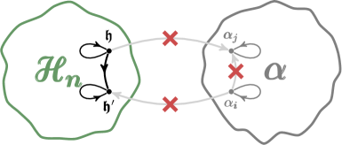
Figure 2: (Color online) This diagram shows works the mutually inaccessible relation for the $\boldsymbol{\alpha}-$states and the states of $\mathscr{H}_{n}$. Those transitions with zero probability are indicated by the crosses (in red).

The linear combination of the elements of $\boldsymbol{\alpha}$, or linear span, contain the states that belong to $\widetilde{\mathscr{H}}_{n^{\prime}}$ but does not belongs to $\mathscr{H}_{n}$, this is the complement of $\mathscr{H}_{n}$ in order to generate $\widetilde{\mathscr{H}}_{n^{\prime}}$, namely $span(\boldsymbol{\alpha})=\widetilde{\mathscr{H}}_{n^{\prime}}\setminus\mathscr{H}_{n}$. For illustrative purposes Fig. 3 shows how is this composition.

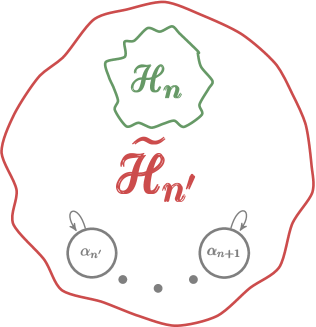
Figure 3: (Color online) This diagram shows how is the composition of $\widetilde{\mathscr{H}}_{n^{\prime}}$ from $\mathscr{H}_{n}$ and a set of ($n^{\prime}{-}n$) redundant states.

VI CONTROL IN QUANTUM SYSTEMS

A remarkable field to apply the presented tools is control theory of quantum systems, in order to implement a quantum simulator conceived as a controllable system whose aim is to mimic the static or dynamical properties of another quantum system [17]. Emphasizing the controllability of a given quantum system, the mapping defined in (30) can be useful to drive the evolution of this system. There are many approaches to control quantum systems, the formalism in this section it starts by choosing the desired state trajectory and then engineers a control that transport the system along this trajectory.

Let’s consider quantum system governs by a time dependent hamiltonian $H(t)$, rigorously speaking this is a time-indexed family of self-adjoint operators on the hilbert space $\mathscr{H}$. Suppose that for each time $t$ its point spectrum is the set $\{\lambda_{n}(t)\}_{n\in I}$ of eigenvalues, in this case all are different, where $I$ is a denumerable set such that $card(I){=}dim(\mathscr{H})$. Also there is an instantaneous basis of orthonormal eigenvectors of $H(t)$ with respect to the inner product $\langle\star|\ast\rangle:\mathscr{H}\times\mathscr{H}\longrightarrow\mathbb{C}$ [2, 3], named $\boldsymbol{\beta}_{t}{=}\{|\varphi_{n}(t)\rangle\}_{n\in I}$. The orthonormality of $\boldsymbol{\beta}_{t}$ is expressed through the inner product $\langle\varphi_{m}|\varphi_{n}\rangle{=}\delta_{mn}$, for all $t{\in}\mathcal{T}$, where $\delta_{mn}$ is the Kroenecker delta which is $1$ if $m{=}n$, and $0$ otherwise.

In general, there is a correspondence to each eigenvalue $\lambda_{n}(t)$ and its eigenspace because by definition $\mathscr{H}_{n,t}{=}\Big{\{|}\varphi_{t}\rangle{\in}\mathscr{H}{:}\,H(t)|\varphi_{t}\rangle{=}\lambda_{n}(t)|\varphi_{t}\rangle\Big{\}}$, for $\lambda_{m}(t){\neq}\lambda_{n}(t)$ then $\mathscr{H}_{m,t}\cap\mathscr{H}_{n,t}=\{0\}$. The hole point spectrum is called non-degenerate, i.e. there are no linearly independent eigenvectors associated with the same eigenvalue. As all eigenvalues are different, mathematically means that $dim(\mathscr{H}_{n,t}){=}1$ for each $n$ and $t$, and physically means if there is no transition between elements of two proper spaces we will have the guarantee that the system will be dominated by a unique eigenvalue. Given that $\boldsymbol{\beta}_{t}$ is a basis for each time $t$, therefore

$$|\varphi(t)\rangle{=}\sum_{n\in I}\xi_{n}(t)|\varphi_{n}(t)\rangle$$ (33)

is a proposed solution of (1) for this time dependent hamiltonian. The functions $\{\xi_{n}(t)\}_{n\in I}$ are obtained replacing the proposed solution in the equation (1)

$$i\partial_{t}\xi_{n}{=}\lambda_{n}\xi_{n}-i\sum_{k\in I}\langle\varphi_{n}|\partial_{t}\varphi_{k}\rangle\xi_{k},$$ (34)

where the time dependence was omitted in order to simplify the notation. In particular, for an initial condition $|\varphi(0)\rangle{\in}\mathscr{H}_{m,0}$ then for $n{\neq}m$: $\xi_{n}(0){=}0$, but $\partial_{t}\xi_{n}(0){=-}\langle\varphi_{n}|\partial_{t}\varphi_{m}\rangle\big{|}_{t=0}$ which is non zero in general. For this reason, even if the system was initially belongs to the eigenspace $\mathscr{H}_{m,0}$, it cannot be guaranteed that a posteriori the state of the quantum system will remain in the same eigenspace, transitions will inevitably take place. If it is intended to control the system so that it remains in a certain eigenspace then let’s see how to express $\langle\varphi_{n}|\partial_{t}\varphi_{m}\rangle$ in another way, since it quantifies the rate of the mentioned transitions. From $H|\varphi_{m}\rangle{=}\lambda_{m}|\varphi_{m}\rangle$, then $\partial_{t}H|\varphi_{m}\rangle{+}H|\partial_{t}\varphi_{m}\rangle{=}\partial_{t}\lambda_{m}|\varphi_{m}\rangle{+}\lambda_{m}|\partial_{t}\varphi_{m}\rangle$, closing on the left with the bra $\langle\varphi_{n}|$ where $n{\neq}m$, finally

$$\langle\varphi_{n}|\partial_{t}\varphi_{m}\rangle=\frac{\langle\varphi_{n}|\partial_{t}H|\varphi_{m}\rangle}{\lambda_{m}{-}\lambda_{n}}.$$ (35)

If $\langle\varphi_{n}|\partial_{t}\varphi_{m}\rangle{\simeq}0$ for $n{\neq}m$ the approximate solution of (34) for each $n{\in}I$ is given by $\xi_{n}(t){\simeq\,}{\exp}\Big{\{}i\int_{0}^{t}\boldsymbol{\big{(}}{-}\lambda_{n}(s){+}i\langle\varphi_{n}(s)|\partial_{s}\varphi_{n}(s)\rangle\boldsymbol{\big{)}}ds\Big{\}}\xi_{n}(0)$, replacing each coordinate $\xi_{n}(t)$ in (33) an approximately solution of (1) is obtained. If $\langle\varphi_{n}|\partial_{t}\varphi_{m}\rangle$ is exactly equal to zero, it corresponds to a non-interaction between states characterised by each states, represented by these instantaneous eigenvector. Only the state corresponds to $n{=}m$ evolves in a non trivial way and decoupled of the rest of states. The quantity $\int_{0}^{t}i\langle\varphi_{n}(s)|\partial_{s}\varphi_{n}(s)\rangle ds$, which appears in addition to the familiar dynamical phase $-\int_{0}^{t}\lambda_{n}(s)ds$ governs the temporal evolution of the state of the system and is also real, see the demonstration in Appendix A2, for this reason can be interpreted as another phase. The relevance of this quantity is such that has its own name, called the Berry phase [18]. This kind of particular phases appears also in classical physics and, given that there is an underlying geometric structure, these are called geometric phases [19].

In order to inhibit the mentioned transitions looking the expression (35) the time variation of the hamiltonian is done slowly enough with respect to the difference of the corresponding eigenvalues. The slowly variation of the hamiltonian is related to a quasistatic process or misnamed in the literature an adiabatic process. There is a connection between the rate of variation of $H$ in order to control the system state permanence in a particular eigenspace $\mathscr{H}_{m,t}$ for a sufficient large time $t$, in this respect. In this section, let’s remember that it is intended that the state trajectory is along the instantaneous eigenstates of the reference hamiltonian $H$.

The above discussion shows that in the natural (i.e. uncontrolled) behaviour of the system it is not the possible guarantee non-transitions between eigenspaces of $H$ to do unless the process is quasistatic, but this problem could be approached in another scenario or quantum basis.

In this section we have been consider an orthonormal basis named dynamical basis $\boldsymbol{\beta}_{t}{=}\{|\varphi_{n}(t)\rangle\}_{n\in I}$ which contains the instantaneous eigenvectors of $H(t)$ and the other scenario will be built on the static or fixed basis $\boldsymbol{\beta}{=}\{|\psi_{n}\rangle\}_{n\in I}$, to write down an unitary operator $\omega{=}\sum_{n\in I}\omega_{n}|\psi_{n}\rangle\langle\varphi_{n}|$, for simplicity the time dependence was omitted for each bra $\langle\varphi_{n}(t)|$. Note that each term in the operator $\omega$ is another operator, $|\psi_{n}\rangle\langle\varphi_{n}|$, associates each ket $|\psi\rangle$ to a new ket $|\psi_{n}\rangle\langle\varphi_{n}|\psi\rangle$ we interpret as the vector multiplied by the scalar. Given that $\omega$ is unitary then $\omega_{n}{=}e^{if_{n}}$ where $f_{n}$ is a real quantity, in other words is the argument or the phase of the complex number $\omega_{n}$. Including the case that $f_{n}$ is a function of time and mapping the hamiltoninan $H$ via $\Omega_{\omega}$ we get

$$\begin{aligned} \Omega_{\omega}(H)&=\omega\,H\,\omega^{\dagger}+i(\partial_{t}\omega)\,\omega^{\dagger}\\ &={\sum}_{n\in I}\boldsymbol{\big{(}}\lambda_{n}+i\langle\partial_{t}\varphi_{n}|\varphi_{n}\rangle-\partial_{t}f_{n}\boldsymbol{\big{)}}\,|\psi_{n}\rangle\langle\psi_{n}|\\ &{+}{\sum}_{\begin{subarray}{c}(m,n)\in I^{2}\\ m\neq n\end{subarray}}{i}\,e^{i(f_{m}-f_{n})}\langle\partial_{t}\varphi_{m}|\varphi_{n}\rangle\,|\psi_{m}\rangle\langle\psi_{n}|,\end{aligned}$$ (36)

where $I^{2}:=I\times I$. Note that $\langle\partial_{t}\varphi_{m}|\varphi_{n}\rangle{=}-\langle\varphi_{m}|\partial_{t}\varphi_{n}\rangle$ thus the first sum in (36) can be drive the state of the system in order to satisfied the desired control goal, if $f_{n}{\equiv}0$ for each $n{\in}I$. Nevertheless the second sum in (36) leads to transitions between states of the system. Any attempt to suppress these transitions requires taking the approximation $\langle\varphi_{m}|\partial_{t}\varphi_{n}\rangle\simeq 0$ for all $m\neq n$ and, given (35), this is equivalent to taking the quasistatic approximation.

Based on the decomposition of the $\Omega_{\omega}$ mapping for a sum of two operators $A$, $B$ and a generic $\omega$ all over $\mathscr{H}$

$$\Omega_{\omega}(A{+}B)=\Omega_{\omega}(A)+\omega\,B\,\omega^{-1}.$$ (37)

Its demonstration follows directly from the definition of the map $\Omega_{\omega}$ (30). Is possible to find another hamiltonian named $\widetilde{H}$ such that $\Omega_{\omega}(H+\widetilde{H})$ can be drive the state of the original system whose hamiltonian is $H$

$$\Omega_{\omega}(H{+}\widetilde{H})\,{=}{\sum}_{n\in I}\boldsymbol{\big{(}}\lambda_{n}+i\langle\partial_{t}\varphi_{n}|\varphi_{n}\rangle\boldsymbol{\big{)}}\,|\psi_{n}\rangle\langle\psi_{n}|.$$ (38)

The details of this procedure are in the Appendix A2.

The idea that we have been pursuing is looking for a hamiltonian $\widetilde{H}$ such that added to our original hamiltonian $H$ which provides an evolution like would be achieved if an adiabatic process were valid for $H$ via $\Omega_{\omega}(H{+}\widetilde{H})$.

In addition to those readers invaded by the anxiety that comes from waiting to finish reading this article to arrive at the aforementioned Appendix A2, here is another shortcut to the closed expression for the additive hamiltonian $\widetilde{H}$

$$\begin{aligned} \widetilde{H}=\,{\sum}_{n\in I}\;&\boldsymbol{\big{(}}\partial_{t}f_{n}+i\langle\partial_{t}\varphi_{n}|\varphi_{n}\rangle\boldsymbol{\big{)}}\,{|\varphi_{n}\rangle}{\langle\varphi_{n}|}+\\ \,{\sum}_{n\in I}\;&i|\partial_{t}\varphi_{n}\rangle\langle\,\varphi_{n}\,|,\end{aligned}$$ (39)

the first sum corresponds to a diagonal operator and the second sum corresponds to a non-diagonal operator.

Note that the phases $\{f_{n}\}_{n\in I}$ in the operator $\omega$ for our exposition are identically zero, but this is not the case in other contexts. In [20] the operator $\omega$ is defined considering a particular static basis defined from the dynamical basis evaluated in $t=0$, i.e. $\boldsymbol{\beta}{:=}\boldsymbol{\beta}_{0}$, and the phases are $f_{n}(t){=}\int_{0}^{t}\boldsymbol{\big{(}}{-}\lambda_{n}(s){+}i\langle\varphi_{n}(s)|\partial_{s}\varphi_{n}(s)\rangle\boldsymbol{\big{)}}ds$.

There is another equivalent expression for $\widetilde{H}$

$$\begin{aligned} \widetilde{H}={\sum}_{n\in I}\;\big{(}\partial_{t}f_{n}\big{)}\,{|\varphi_{n}\rangle}{\langle\varphi_{n}|}&+\\ \;{\sum}_{\begin{subarray}{c}(m,n)\in I^{2}\\ m\neq n\end{subarray}}i\frac{\langle\varphi_{m}|\partial_{t}H|\varphi_{n}\rangle}{\lambda_{n}{-}\lambda_{m}}&{|\varphi_{m}\rangle\langle\varphi_{n}|},\end{aligned}$$ (40)

again, the first sum corresponds to a diagonal operator and the second sum corresponds to a non-diagonal operator.

The methodology which was described is called an adiabatic shortcut and in particular we have argued the transitionless driving protocol, for a clearly mathematical explanation see [20] and for an equivalent approach, called counter-diabatic see [21]. While in [22] is possible to find and use a time invariant operator to solve (1) via a similar reverse engineering protocol. Remark that transitionless driving is one of the adiabatic shortcut protocols [20], but there are many others summarized in [23, 24].

On the other hand, the transformation under $\Omega_{\omega}$ of $H$ multiplied by a number $u\in\mathbb{C}$ is

$$\Omega_{\omega}(u\,H)=u\,\Omega_{\omega}(H)-i(u-1)(\partial_{t}\omega)\omega^{-1}.$$ (41)

The transformation under $\Omega_{\omega}$ of a finite sum of hamiltonian operators is given

$$\Omega_{\omega}\boldsymbol{\Big{(}}\sum_{k=1}^{N}H_{k}\boldsymbol{\Big{)}}=\sum_{k=1}^{N}\Omega_{\omega}(H_{k})-i(N-1)(\partial_{t}\omega)\omega^{-1}.$$

Another result of $\Omega_{\omega}$ is the invariance under a particular linear combination. If the departure hamiltonian $H$ is given by a convergent linear combination of hamiltonians $\{H_{k}\}_{k\in J}$, where $J$ is a denumerable index set, $\sum_{k\in J}u_{k}{=}\,u$, when $u$ can be time dependent, then

$$\Omega_{\omega}\boldsymbol{\Big{(}}\sum_{k\in J}u_{k}\,H_{k}\boldsymbol{\Big{)}}=\sum_{k\in J}u_{k}\,\Omega_{\omega}(H_{k})-i(u-1)(\partial_{t}\omega)\omega^{-1},$$

in particular, if $u\neq 0$ the parameters $\{w_{k}\}_{k\in J}$ can be rewritten as $u_{k}=u\,w_{k}$ and conclude that

$$\Omega_{\omega}\boldsymbol{\Big{(}}\sum_{k\in J}w_{k}\,H_{k}\boldsymbol{\Big{)}}=\sum_{k\in J}w_{k}\,\Omega_{\omega}(H_{k}),$$ (42)

because $\{w_{k}\}_{k\in J}$ satisfied $\sum_{k\in J}w_{k}{=}1$. In other words, can be considered as weights. The expression (42) is preserved even if the weights are signed $w_{k}{\geq}0$ for all $k{\in}J$, in this case is called a convex combination. This quantities called weights $\{w_{k}\}_{k\in J}$ are eventually responsible to control the time spend to simulate each part of the convex sum [3, 11]. In this context, the invariance under convex combination allows to transform each hamiltonian control problem $\{w_{k},H_{k}\}_{k\in J}$ into another $\{w_{k},\Omega_{\omega}(H_{k})\}_{k\in J}$ but preserving the weights.

VII Swallowing Algorithm

Inspired in the algorithm presented in [25] conformed by a sequence of unitary transformation, there is a possibility to reduce a sum of $N$ hamiltonian operators from one hamiltonian operator by a finite sequence of operators $\{\omega_{k}\}_{k=1,\,\cdots,N}$ non necessarily unitary and its implementation of the corresponding sequence $\{\Omega_{\omega_{k}}\}_{k=1,\,\cdots,N}$.

Once more, based on the decomposition of the $\Omega_{\omega}$ mapping exposed in (37), if also demand that $\Omega_{\omega}(A){=}0$ we can reduce (37) to $\Omega_{\omega}(A+B){=}\omega\,B\,\omega^{-1}$. Suppose we are interested in studying the temporal evolution of a quantum systems whose hamiltonian is $\sum_{j=1}^{N}H_{j}$ using the following procedure, we can swallow each term of this sum sequentially. As these are bounded Hamiltonian operators, then it will be lawful to demand for an invertible operator $\omega_{1}$ that $\Omega_{\omega_{1}}(H_{1}){=}0$, what is achieved if $\omega_{1}$ satisfies $i\,\dot{\omega}_{1}{=}-\omega_{1}\,H_{1}$. Therefore ${\Omega_{\omega_{1}}}\boldsymbol{\Big{(}}\sum_{j=1}^{N}H_{j}\boldsymbol{\Big{)}}{=}\sum_{j=2}^{N}H^{(1)}_{j}$, with $H^{(1)}_{j}{:=}\omega_{1}\,H_{j}\,\omega_{1}^{-1}$. It can be seen that $\Omega_{\omega_{1}}$ takes a sum of $N$ hamiltonians and returns a sum of $N-1$ hamiltonians which none of these are exactly any of those original sum but are equivalent via a similarity transformation given by $\omega_{1}$. This procedure can be repeated $N-1$ times until leaving a single hamiltonian or taking one more step the $N$-step and concluding the swallowing task leaving an identically null hamiltonian.

Firstly we define the similarity transformations of the hamiltonians for each $j,k\in\{1,\cdots,N\}$

$$\begin{aligned} H_{j}^{(k)}&{:=}\,\omega_{k}\cdots\omega_{1}H_{j}(\omega_{k}\cdots\omega_{1})^{-1},\\ H_{j}^{(0)}&{:=}H_{j},\end{aligned}$$ (43)

where the second expression denotes the starting point, $H_{j}^{(0)}$, of each hamiltonian $H_{j}$ to initialize the algorithm. We have used a compact notation $\omega_{k}\cdots\omega_{1}$ to denote the ordered composition of this operators.

Secondly, we suppose a sequence of invertible operators $\{\omega_{k}:k=1,{\cdots},N\}$ such that

$$\Omega_{\omega_{k}}\Big{(}H_{k}^{(k-1)}\Big{)}=0.$$ (44)

Finally, before giving an account of the swallowing algorithm, let us note the following recurrence relationship that will be useful to construct it

$$H_{j}^{(k)}=\omega_{k}\,H_{j}^{(k-1)}\omega_{k}^{-1}$$ (45)

Then we can think of a protocol of $N{-}1$ steps (or $N$ steps if we want total swallowing) so that, using (37), (43), (44) and (45) we can say that $k$-step is given by

$$\Omega_{\omega_{k}\cdots\,\omega_{1}}\Big{(}\sum\nolimits_{j=1}^{N}H_{j}\Big{)}=\sum\nolimits_{j=k+1}^{N}H^{(k)}_{j}$$ (46)

for each $k{=}1,{\cdots},N$. The left member is designed to swallow $k$ addends, so for the original $N$ addends will remain $N{-}k$.

Let’s see the proof by finite induction on $k$. The first step $k=1$ is true from (37) with $A{=}H_{1}$ y $B{=}\sum_{j=2}^{N}H_{j}$, (43) and (44). Taking the $k$-step in (46) and apply $\Omega_{\omega_{k+1}}$ then

$$\begin{aligned} \Omega_{\omega_{k+1}}\bigg{(}\Omega_{\omega_{k}\cdots\,\omega_{1}}\Big{(}\sum_{j=1}^{N}H_{j}\Big{)}\bigg{)}&=\Omega_{\omega_{k+1}}\bigg{(}\sum_{j=k+1}^{N}H^{(k)}_{j}\bigg{)}\\ \Omega_{\omega_{k+1}\omega_{k}\cdots\,\omega_{1}}\Big{(}\sum_{j=1}^{N}H_{j}\Big{)}&=\Omega_{\omega_{k+1}}\Big{(}H^{(k)}_{k+1}\Big{)}+\\ &+\sum_{j=k+2}^{N}\omega_{k+1}H^{(k)}_{j}\omega_{k+1}^{-1}\\ \Omega_{\omega_{k+1}\cdots\,\omega_{1}}\Big{(}\sum_{j=1}^{N}H_{j}\Big{)}&=\sum_{j=k+2}^{N}H^{(k+1)}_{j}\end{aligned}$$ (47)

which is exactly the statement which appear in (46) but for the $(k{+}1)$-step.

Inasmuch as the map $\Omega_{\omega}$ is invertible, then the presented protocol connection is in both ways: from a sum of $N$-hamiltonians and a unique hamiltonian and vice versa. We have omitted the existence of this reverse procedure from the title of the section, since it is a digestive process that does not evoke good mental images or pleasant sensations for the reader of this work.

VIII Final observations

The aim of present work it was to prove that there is a way to modify the behavior of a known quantum system, in order to get information of another quantum system that, at least, has a difficulty to be resolved directly.

Even when the state space of each Hilbert space has different cardinality, it is still possible to establish a link via a local transformation. This connection could be used including an eventually $t-$dependence of any of these hamiltonian operators.

In summary, we have shown how for a given pair of quantum systems, finite-dimensional Hilbert spaces and its respective hamiltonian: $(\mathscr{H},H)$ and $(\mathscr{H}^{\prime},H^{\prime})$ they could be linked via gauge (local) transformations $\omega$, that allow us to obtain $H^{\prime}$ from $H$, via $\Omega_{\omega}$.

In addition, this method allows us to address a new problem from another known one, using a non-local modulation ($\omega$) of the well-known solution $|\varphi\rangle$, following (30). We have not only shown that this is feasible to do through formal and constructive proof of the existence of that $\omega$. But also we have indicated what is the right way to do it: should be across a linear and local (i.e. time-dependent) operation.

Respect to the simulation of a quantum system Q^′ we search for some other system that imitates the behavior of Q as well as possible. In other words, we must perform a casting call of quantum systems or actors which can be very limited, because it is a hard task to find another Q one to simulate Q^′. We wanted to use this equivalence between quantum systems to simulate another quantum system connected with Q^′. But when we said another, we want to say any other quantum system which is connected with Q^′ through $\omega$. The map $\Omega_{\omega}$ applied to a given hamiltonian $H$ in (10) works as makeup that allows any actor Q, to simulate the first quantum system Q^′, a priori, if Q is connected with Q^′ through $\omega$. Following the metaphor, the equivalence between this quantum systems expands that catalogue of actors that can make a good performance in order to mimic another quantum system and becoming that casting call, a priori more efficient.

Given that the equivalence relation $\sim$ defines an equivalent class, see Appendix, the set of all transformations forms a guild of actors capable of simulating, a priori, any quantum system of such systems conglomerate, which can be fully explored by such set of transformations. In particular, the subset of mapping wich $\omega$ unitary forms a conservative guild of actors capable of simulating quantum systems with selfadjoint hamiltonian.

Regarding to control theory of quantum systems we have shown that there is a strong connection with our mapping $\Omega_{\omega}$ since it can be implemented to design temporal evolutions required a priori from a primal hamiltonian $H(t)$. We have dealt with the case of an orthonormal basis of eigenvectors of $H(t)$ whose point spectrum is non-degenerate transferring this problem to a static basis also orthonormal. From the concrete $\omega$ can be seen that both bases, dynamical and statical are bi-orthonormal, i.e. $\langle\psi_{n}|\varphi_{m}\rangle{=}\delta_{nm}$. This property allows to guarantee the original identification between each vector of the dynamical basis with the corresponding eigenvalue also for the statical basis. This can be generalized introducing a more general $\omega$ operators.

A final comment in this regard could be the implementation of the formal equivalence between quantum and classical systems proposed in [26] in order to simulate quantum systems through specific circuits. The advantage of using such classical systems is that their controllability is simpler than for quantum systems in general, in order to adequately guide its temporal evolution. This implementation open the possibility to expands this catalogue of actors capable of simulating the quantum system $Q$ even more with classical actors, who usually do not play that role.

Further applications of this methodological connection could be applied to perform computer simulation of quantum systems in a new way.

Competing interest

The author declares that there are no competing interests.

Appendix

*

A1. Some structural properties of map $\boldsymbol{\Omega_{\omega}}$

$\bullet$ MAPPING COMPOSITION

We composed two transformations $\Omega_{\omega}\circ\,\Omega_{\omega}^{\prime}$ with $\omega$ and $\omega^{\prime}$ are nonsingular and then prove that

$$\Omega_{\omega}\circ\Omega_{\omega^{\prime}}(H)=\Omega_{\omega\omega^{\prime}}(H).$$ (1)

for all $H$. We calculate directly $\Omega_{\omega}\circ\,\Omega_{\omega^{\prime}}(H)$, denoting it by $\boldsymbol{\square}=\Omega_{\omega}\circ\,\Omega_{\omega^{\prime}}(H)$

$$\boldsymbol{\square} {=}\Omega_{\omega}\boldsymbol{(}\omega^{\prime}H\omega^{\prime-1}{+}i(\partial_{t}\omega^{\prime})\omega^{\prime-1}\boldsymbol{)}$$

$${=}\omega\big{[}\omega^{\prime}H\omega^{\prime-1}{+}i(\partial_{t}\omega^{\prime})\,\omega^{\prime-1}\big{]}\omega^{-1}{+}i(\partial_{t}\omega)\,\omega^{-1}$$

$${=}\omega\,\omega^{\prime}H(\omega\,\omega^{\prime})^{-1}{+}i\omega(\partial_{t}\omega^{\prime})(\omega\,\omega^{\prime})^{-1}{+}i(\partial_{t}\omega)\,(\omega^{\prime}\omega^{\prime-1})\,\omega^{-1}$$

$${=}\omega\,\omega^{\prime}H(\omega\,\omega^{\prime})^{-1}{+}i\omega(\partial_{t}\omega^{\prime})(\omega\,\omega^{\prime})^{-1}{+}i(\partial_{t}\omega)\,\omega^{\prime}(\omega\,\omega^{\prime})^{-1}$$

$${=}\omega\omega^{\prime}H(\omega\,\omega^{\prime})^{-1}{+}i\partial_{t}(\omega\,\omega^{\prime})(\omega\,\omega^{\prime})^{-1}$$

$$\boldsymbol{\square} {=}\Omega_{\omega\omega^{\prime}}(H).$$

This completes the demonstration of (1): $\Omega_{\omega}{\circ}\;\Omega_{\omega^{\prime}}{=}\;\Omega_{\omega\omega^{\prime}}$ and expression (12) is satisfied.

$\bullet$ INVERSE MAPPING

We calculate explicitly $\Omega_{\omega^{-1}}(H)$ and then prove that

$$\Omega_{\omega^{-1}}(H)=\Omega_{\omega}^{-1}(H),$$ (2)

for all $H$. Let’s calculate the left hand of (2)

$$\Omega_{\omega^{-1}}(H) =\omega^{-1}H\omega+i(\partial_{t}\omega^{-1})\omega$$

$$=\omega^{-1}H\omega+i(\partial_{t}\omega^{-1})\omega$$

$$\Omega_{\omega^{-1}}(H) =\omega^{-1}H\omega-i\omega^{-1}\partial_{t}\omega.$$

Finally we check directly that $\Omega_{\omega^{-1}}$ is equal to $\Omega_{\omega}^{-1}$, if for all $H$ we take $\boldsymbol{\hexagon}=\Omega_{\omega}\circ\Omega_{\omega^{-1}}(H)$ and calculate

$$\boldsymbol{\hexagon} =\Omega_{\omega}(\omega^{-1}H\omega-i\omega^{-1}\partial_{t}\,\omega)$$

$$=\omega(\omega^{-1}H\omega-i\omega^{-1}\partial_{t}\omega)\,\omega^{-1}+i(\partial_{t}\omega)\,\omega^{-1}$$

$$=\omega\,\omega^{-1}H\omega\,\omega^{-1}-i\omega\,\omega^{-1}(\partial_{t}\omega)\,\omega^{-1}+i(\partial_{t}\omega)\,\omega^{-1}$$

$$=H-i(\partial_{t}\omega)\,\omega^{-1}+i(\partial_{t}\omega)\,\omega^{-1}$$

$$\boldsymbol{\hexagon} =H,$$

where $\partial_{t}(\omega^{-1}\omega){=}\,\boldsymbol{0}$ then $\partial_{t}(\omega^{-1})\,\omega=-\omega^{-1}\partial_{t}\,\omega$. This completes the demonstration of (2): $\Omega_{\omega^{-1}}=\Omega_{\omega}^{-1}$ and expression (16) is satisfied.

$\bullet$ AN EQUIVALENCE RELATION DEFINED BY $\Omega_{\omega}$

We say that the map $\Omega_{\omega}$ defined an equivalence relation between the space of operators defined on isomorphic Hilbert spaces. For a given two hamiltonian operators $(H,H^{\prime})$ we can define a relation between them

$$H^{\prime}\sim H\Longleftrightarrow\exists\,\omega:H^{\prime}=\Omega_{\omega}(H),$$ (3)

where $\Omega_{\omega}(H):=\omega H\omega^{-1}+i(\partial_{t}\,\omega)\omega^{-1}$ and $\omega$ is a nonsingular operator. The relation (3) between two operators $H^{\prime}\sim H$ is an equivalence in the sense that for all operators $H,H^{\prime},H^{\prime\prime}$ the following properties are true:

$$(\boldsymbol{R})\quad H{\sim}H\quad(\mathit{reflexivity})$$

$$(\boldsymbol{S})\quad H{\sim}H^{\prime}\Longrightarrow H^{\prime}{\sim}\,H\quad(\mathit{symmetry})$$

$$(\boldsymbol{T})\quad H^{\prime\prime}{\sim}\,H^{\prime}\;{\scriptstyle\land}\;H^{\prime}{\sim}\,H\Longrightarrow H^{\prime\prime}{\sim}\,H\quad(\mathit{transitivity})$$

The first assertion ($\boldsymbol{R}$) is true from the identity operator $\omega=I$ and by definition $\Omega_{I}(H)=H$. The assertion ($S$) is also true from the existence of the inverse operator $\omega^{-1}$ and construct through (2) the inverse connection $H^{\prime}\sim H$. The last assertion ($T$) is true from the composed transformation of non singular operator $\omega=\omega^{\prime\prime}\omega^{\prime}$ and (1), such that $H^{\prime\prime}=\Omega_{\omega^{\prime\prime}}(H^{\prime})$ and $H^{\prime}=\Omega_{\omega^{\prime}}(H)$, then $H^{\prime\prime}=\Omega_{\omega^{\prime\prime}}(\Omega_{\omega^{\prime}}(H))=\Omega_{\omega}(H)$. Finally, we arrive to $H^{\prime\prime}\sim H$.

A2. some required additional proofs

We start to prove (34), from $|\varphi(t)\rangle{=}\sum_{n\in I}\xi_{n}(t)|\varphi_{n}(t)\rangle$, taking the partial time derivative and use the Schrödinger equation (1) $\sum_{n\in I}i(\partial_{t}\xi_{n})\,|\varphi_{n}\rangle+i(\xi_{n})\,|\partial_{t}\varphi_{n}\rangle{=}\sum_{n\in I}\lambda_{n}\xi_{n}\varphi_{n}$ then close from the left with a bra $\langle\varphi_{k}|$ and using the orthonormal character of the dynamical basis $\boldsymbol{\beta}_{t}$ finally obtain $i\partial_{t}\xi_{k}+i\sum_{n{\in}I}\xi_{n}\langle\varphi_{k}|\partial_{t}\varphi_{n}\rangle{=}\lambda_{k}\xi_{k}$. Note that $\langle\varphi_{m}|\varphi_{n}\rangle{=}\delta_{mn}$ for all $t$, then $\langle\partial_{t}\varphi_{m}|\varphi_{n}\rangle{=-}\langle\varphi_{m}|\partial_{t}\varphi_{n}\rangle$. Finally we get $\langle\varphi_{n}|\partial_{t}\varphi_{n}\rangle{{}^{*}}{=}\langle\partial_{t}\varphi_{n}|\varphi_{n}\rangle{=-}\langle\varphi_{n}|\partial_{t}\varphi_{n}\rangle$, then $\int_{0}^{t}i\langle\varphi_{n}(s)|\partial_{s}\varphi_{n}(s)\rangle ds$ is a real quantity.

In order to arrive at (36) we start from

$$\begin{aligned} \Omega_{\omega}(H)&=\omega\,H\,\omega^{\dagger}+i(\partial_{t}\omega)\,\omega^{\dagger},\\ &={\sum}_{n\in I}\boldsymbol{\big{(}}\lambda_{n}+{i}(\partial_{t}\omega_{n})\omega_{n}^{*}\boldsymbol{\big{)}}\,|\psi_{n}\rangle\langle\psi_{n}|\\ &+\;{\sum}_{(m,n)\in I^{2}}{i}\omega_{m}\omega_{n}^{*}\langle\partial_{t}\varphi_{m}|\varphi_{n}\rangle\,|\psi_{m}\rangle\langle\psi_{n}|,\\ \Omega_{\omega}(H)&={\sum}_{n\in I}\boldsymbol{\big{(}}\lambda_{n}-\partial_{t}f_{n}\boldsymbol{\big{)}}\,|\psi_{n}\rangle\langle\psi_{n}|\\ &+\;{\sum}_{(m,n)\in I^{2}}{i}\,e^{i(f_{m}-f_{n})}\langle\partial_{t}\varphi_{m}|\varphi_{n}\rangle\,|\psi_{m}\rangle\langle\psi_{n}|,\\ \end{aligned}$$

and extracting the term that corresponds to $n{=}m$ of the double sum, finally obtain (36).

To prove (39) the procedure is as follows: using (37) $\Omega_{\omega}(H{+}\widetilde{H}){=}\omega H\omega^{\dagger}{+}\Omega_{\omega}(\widetilde{H})$ and using the defined operator ${\omega}$ then $\omega H\omega^{\dagger}{=}\sum_{n\in I}\lambda_{n}\,|\psi_{n}\rangle\langle\psi_{n}|$, so it only remains to find a hamiltonian $\widetilde{H}$ so that from the requirement established by (38) then $\Omega_{\omega}(\widetilde{H}){=}\sum_{n\in I}i\,\boldsymbol{(}\langle\partial_{t}\varphi_{n}|\varphi_{n}\rangle\boldsymbol{)}\,|\psi_{n}\rangle\langle\psi_{n}|$. Finally obtain this additive hamiltonian $\widetilde{H}$ via the inverse mapping of $(\Omega_{\omega})^{-1}$ using (2) we calculate

$$\begin{aligned} \widetilde{H}&=\Omega_{\omega^{-1}}\boldsymbol{\bigg{(}}\sum_{n\in I}i\,\boldsymbol{(}\langle\partial_{t}\varphi_{n}|\varphi_{n}\rangle\boldsymbol{)}\,|\psi_{n}\rangle\langle\psi_{n}|\boldsymbol{\bigg{)}},\\ &=\sum_{n\in I}i\,\omega{{}^{\dagger}}\Big{[}\boldsymbol{(}\langle\partial_{t}\varphi_{n}|\varphi_{n}\rangle\boldsymbol{)}\,|\psi_{n}\rangle\langle\psi_{n}|\Big{]}\omega+i\partial_{t}(\omega^{\dagger})\omega,\\ \widetilde{H}&=i\,{\sum}_{n\in I}\;|\partial_{t}\varphi_{n}\rangle\langle\varphi_{n}|+\boldsymbol{\big{(}}\langle\partial_{t}\varphi_{n}|\varphi_{n}\rangle{-}i\partial_{t}f_{n}\boldsymbol{\big{)}}\,{|\varphi_{n}\rangle}{\langle\varphi_{n}|},\end{aligned}$$

which is exactly (39).

References

- [1] Feynman, R.P.; Simulation Physics with Computers, Int. J. Theor. Phys. 21, (1982).
- [2] Brian C., Hall; Quantum Theory for Mathematicians, Springer (2013)
- [3] Reed, M., Simon, B., Methods of Modern Mathematical Physics. Volume 1-4, Academic Press (1975).
- [4] Dirac, P.A.M.; The principles of Quantum Mechanics, Oxford University Press, (1958), 4∘ed.
- [5] Varadarajan, V.S.; Formal Reduction Theory of Meromorphic Differential Equations: A Group Theoretic view, Pacific. J. Math. Vol. 109, 1, 180 (1986).
- [6] Varadarajan, V.S.; Linear Meromorphic Differential Equations: A Modern Point of View, Am. Math. Soc. Vol. 33, 142 (1996).
- [7] Varadarajan, V.S.; Vector Bundles and Connections in Physics and Mathematics: Some Historical Remarks, Trends Math, 502541 (2003).
- [8] Mostafazadeh, A.; Quantum canonical transformations and exact solution of the Schrödinger equation, J. Math. Phys., 38, (1997).
- [9] Mostafazadeh, A.; Time dependent diffeomorphisms as quantum canonical transformations and the time dependent harmonic oscillator, J. Phys. A, 31, , 1998).
- [10] Mostafazadeh, A.; Geometric phases, symmetries of dynamical invariants, and exact solution of the Schrodinger equation, J. Phys. A, 34, (2001)
- [11] Jones, C.K.R.T., Kirchgraber U., Walther, H. O. Dynamics Reported: Expositions in Dynamical Systems 5, Springer-Verlag (1996).
- [12] Suzuki, M.; Generalized Trotter’s Formula and Systematic Approximants of Exponential Operators and Inner Derivations with Applications to Many-Body Problems, Comm. Math. Phys., 51 (1976).
- [13] Suzuki, M.; Fractal decomposition of exponential operators with applications to many-body theories and Monte Carlo simulations, Phys. Lett. A, 146, , (1990).
- [14] Nielsen, M. A., Chuang, I. L.; Quantum Computation and Quantum Information, Cambridge University Press (2011).
- [15] Benenti, G., Casati, G., Strini, G.;. Principles of Quantum Computation And Information, Vol I and II, World Scientific Publishing Co., Inc. (2007).
- [16] Magnus, W.; On the exponential solution of differential equations for a linear operator. Comm. Pure and Appl. Math. VII 4, (1954).
- [17] Georgescu, I.M., Ashhab, S., Nori, F.; Quantum simulation, Rev. Mod. Phys. 86, (2014).
- [18] Berry, M. V.; Quantal Phase Factors Accompanying Adiabatic Changes, Proc. R. Soc. Lond. A 392, (1984).
- [19] Shapere, A. and Wilczek, F. Geometric Phases in Physics, Singapore: World Scientific(1989).
- [20] Berry, M. V.; Transitionless quantum driving, J. Phys. A: Math. Theor. 42, 365303 (2009).
- [21] Demirplak, M., Rice, S.A.; Adiabatic population transfer with control fields, J. Phys. Chem. A 107, 9937 (2003).
- [22] Lewis, H.R.; Riesenfeld, W.B.; An exact quantum theory of the time-dependent harmonic oscillator and of a charged particle in a time-dependent electromagnetic field., J. Math. Phys. 10, 1458 (1969).
- [23] Guéry-Odelin, D.; et.al.; Shortcuts to adiabaticity: Concepts, methods, and applications, Rev. Mod. Phys. 91, 045001 (2019).
- [24] Torrontegui, E.; et.al.; Shortcuts to adiabaticity, Advances in atomic, molecular, and optical physics, 62, Elsevier, (2013).
- [25] Berry, M. V.; Quantum Phase Corrections from Adiabatic Iteration, Proc. R. Soc. Lond. A 414, (1987).
- [26] Caruso M., Fanchiotti H., García Canal C. A., Mayosky M. and Veiga A.; The quantum CP-violating kaon system reproduced in the electronic laboratory, Proc. R. Soc. A.472, 20160615 (2016).