Figure 1. Our NeuralClothSim is the first neural cloth simulator representing surface evolution as a coordinate-based implicit neural deformation field (NDF). It is supervised for each target scenario (specified by material properties and external forces) with the laws of the Kirchhoff-Love thin shell theory with non-linear strain. Once trained, the simulation can be queried continuously and consistently in space and time enabling different frame rates (bottom left) and spatial resolutions (bottom middle). Moreover, NeuralClothSim is differentiable and can incorporate learnt priors such as material properties that can be edited at test time (bottom right).

NeuralClothSim: Neural Deformation Fields Meet the Kirchhoff-Love Thin Shell Theory

Abstract.

Cloth simulation is an extensively studied problem, with a plethora of solutions available in computer graphics literature. Existing cloth simulators produce realistic cloth deformations that obey different types of boundary conditions. Nevertheless, their operational principle remains limited in several ways: They operate on explicit surface representations with a fixed spatial resolution, perform a series of discretised updates (which bounds their temporal resolution), and require comparably large amounts of storage. Moreover, back-propagating gradients through the existing solvers is often not straightforward, which poses additional challenges when integrating them into modern neural architectures. In response to the limitations mentioned above, this paper takes a fundamentally different perspective on physically-plausible cloth simulation and re-thinks this long-standing problem: We propose NeuralClothSim, i.e., a new cloth simulation approach using thin shells, in which surface evolution is encoded in neural network weights. Our memory-efficient and differentiable solver operates on a new continuous coordinate-based representation of dynamic surfaces, i.e., neural deformation fields (NDFs); it supervises NDF evolution with the rules of the non-linear Kirchhoff-Love shell theory. NDFs are adaptive in the sense that they 1) allocate their capacity to the deformation details as the latter arise during the cloth evolution and 2) allow surface state queries at arbitrary spatial and temporal resolutions without retraining. We show how to train our NeuralClothSim solver while imposing hard boundary conditions and demonstrate multiple applications, such as material interpolation and simulation editing. The experimental results highlight the effectiveness of our formulation and its potential impact.

1. Introduction

Realistic cloth simulation is a central, long-standing and challenging problem in computer graphics. It arises in game engines, computer animation, movie production, and digital art, to only name a few areas. To date, it has been mostly addressed with physics-based simulators operating on explicit geometric representations, i.e., meshes and particle systems.

While recent physics-based simulators (Guo et al., 2018; Wang, 2021; Li et al., 2022, 2018, 2020) can produce realistic 3D simulations that obey various types of boundary conditions, e.g., gravity, wind, interactions with objects, and consider secondary effects, e.g., self-collisions, their operational principle remains limited in several ways. First, they work on explicit surface representations, e.g., meshes, as well as fixed time integration steps and, therefore, inherently assume a pre-defined spatial and temporal resolution that cannot be easily changed once the simulation is accomplished. Moreover, it is difficult to edit the output 3D state without re-running the simulation (e.g., changing the cloth geometry or fabric type). Moreover, re-running with different meshing and frame rates leads to different simulation outcomes, which is often problematic for downstream applications. Second, many of them are not trivially differentiable, which could be a disadvantage when combined with modern neural architectures. Third, explicit geometric representations require notoriously large amounts of storage for the simulation outcomes: The memory size grows 1) linearly with the number of points and 2) linearly with the number of meshes in a sequence.

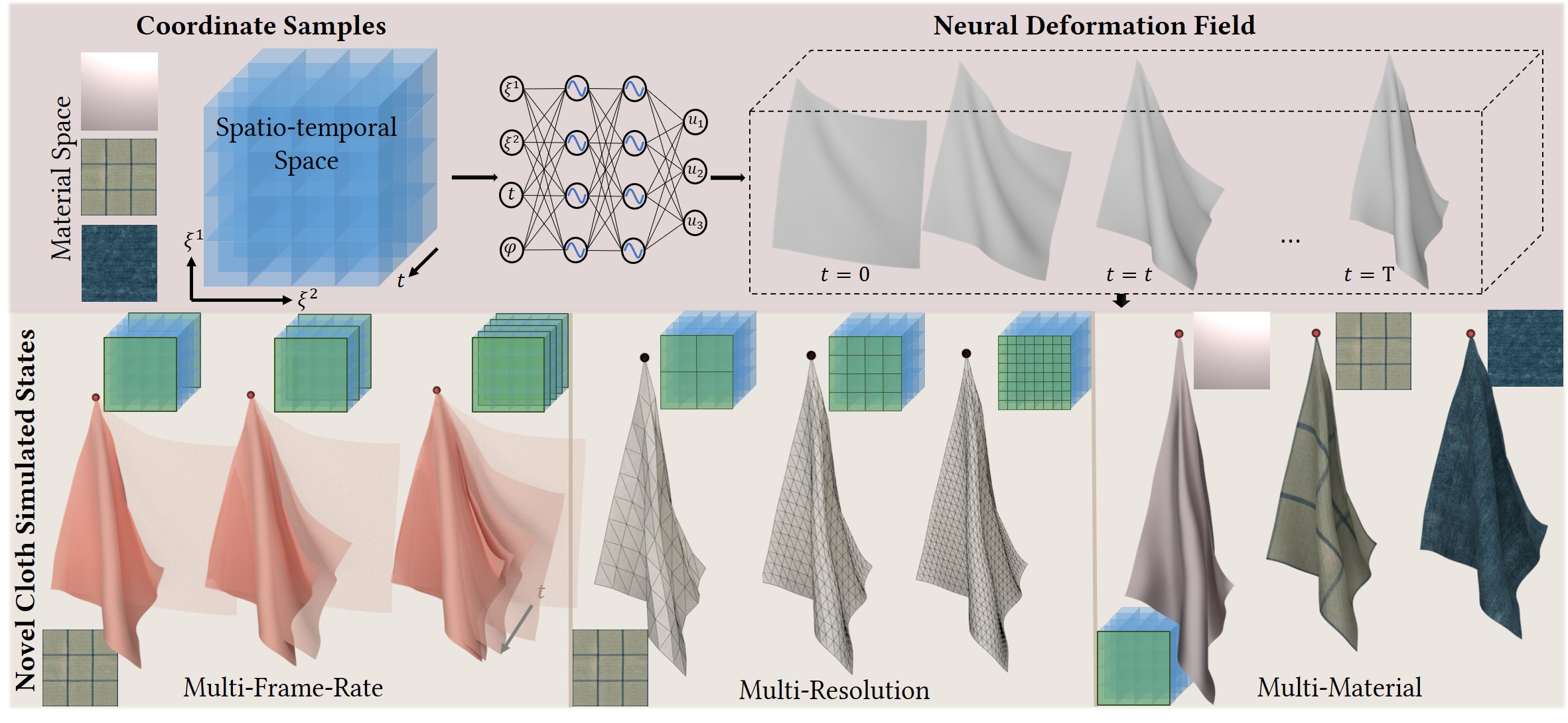
The recent advances in physics-informed neural networks (Raissi et al., 2019; Hao et al., 2022) as well as the success of neural fields (Mildenhall et al., 2020; Xie et al., 2022), makes us question if continuous coordinate-based representations can alleviate these limitations. All these considerations motivate us to rethink the fundamentals of physically-plausible cloth simulation and we introduce a new approach for cloth simulation, in which the surface evolution is encoded in neural network weights. The proposed neural architecture is coordinate-based and has multiple advantages compared to previous simulators; see Fig. 1 for an overview. Our neural fields are adaptive, i.e., the parameters are used to encode the deformations as they occur. As a matter of efficiency, we neither need to know the resolution in advance before the simulation, nor we require complex re-meshing schemes during the simulation (Narain et al., 2012). Realistic cloth simulation requires modelling geometric non-linearities and non-linear elasticity. It involves large bending deformations and rigid transformations leading to non-linear point displacements. To efficiently model this, we rely on neural networks as they can represent complex non-linear functions.

In contrast to previous works that rely on isogeometric analysis (Lu and Zheng, 2014), loop (Thomaszewski et al., 2006; Grinspun et al., 2002) or the Catmull-Clark (Guo et al., 2018) subdivision surface algorithms for modelling Kirchhoff-Love shell theory, we model the evolution of thin shells through deep neural networks. Shell theory studies the dynamics of surfaces subject to boundary conditions such as forces and linear or rotational moments. It was developed in the late 19th century by A. E. H. Love as an extension of beam theory using Kirchhoff assumptions. Nowadays, it is often used in applied mechanics and engineering to model shell structures (Kiendl et al., 2009; Behzadinasab et al., 2022), though its applications in computer graphics for explicit cloth simulation are also known (Thomaszewski et al., 2006; Kopanicakova et al., 2019). In contrast, this paper combines Kirchhoff-Love shell theory with the learning of implicit neural representations, i.e., time-dependent 3D deformation fields representing/encoding cloth dynamics. During training, our formulation supervises a neural deformation field (NDF). In summary, our core technical contributions are as follows:

• A new continuous coordinate-based neural representation—that we call neural deformation fields (Sec. 4.1)—and NeuralClothSim, i.e., a new continuous solver for cloth simulation based on thin shell theory (Sec. 3). Our solver accepts boundary conditions such as external forces or guiding motions (Sec. 4.2).

• Physically-principled modelling of thin shell’s evolution through Kirchhoff-Love theory that supervises the neural deformation fields (Sec. 4.3). Upon convergence, our method encodes the learnt time-dependent states of the thin shell that can be queried continuously in space and time.

• Applications of the proposed neural simulator, including conditioning on material properties, material interpolation (Sec. 4.4) and fast editing of simulations according to updated simulation parameters (Sec. 4.5).

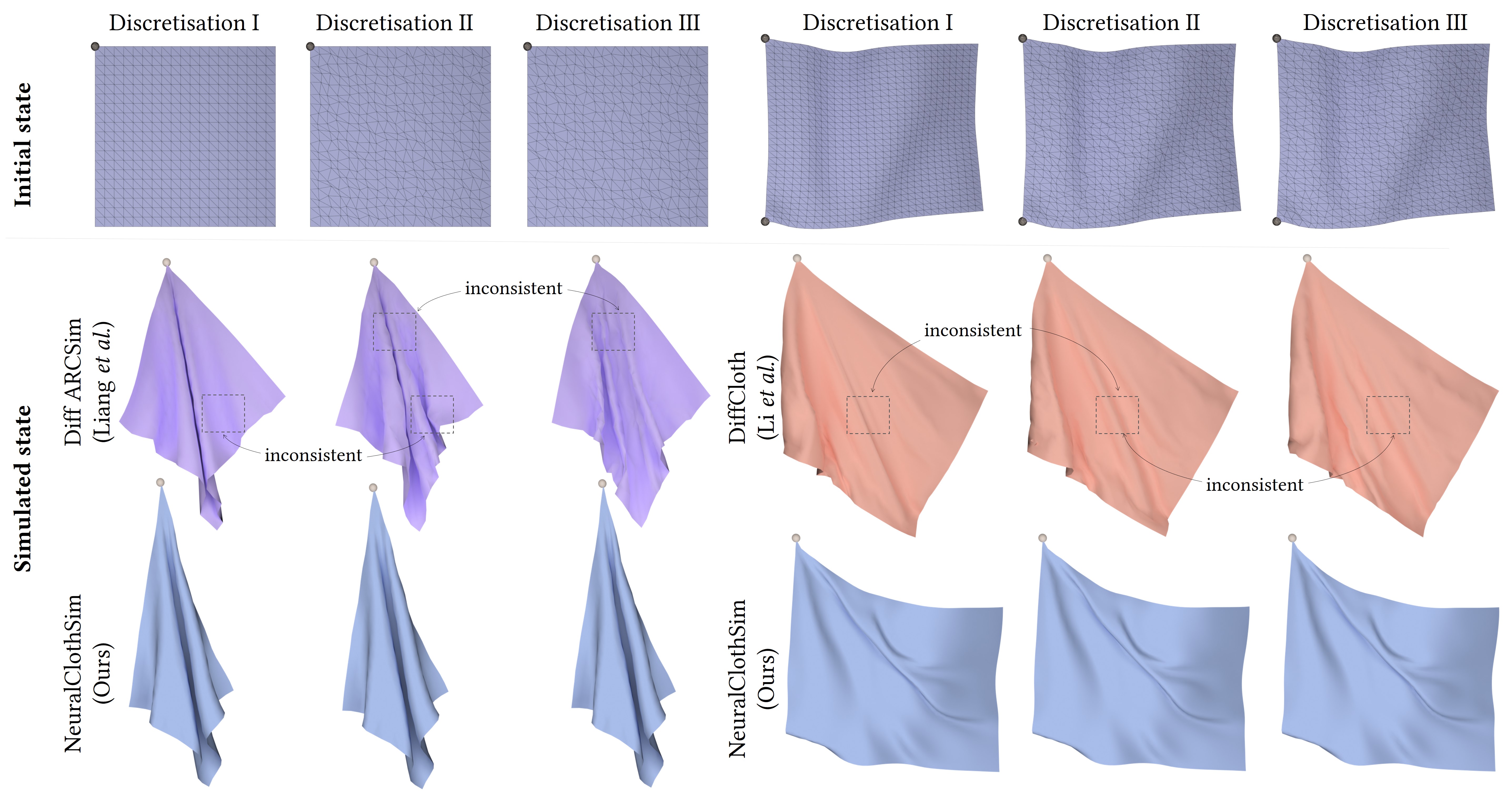
Our method is differentiable by design. Differentiability is beneficial for various applications, such as optimisation, inverse design, system identification, or control. In contrast to some traditional simulators (Liang et al., 2019; Li et al., 2022) that are sensitive to the finite element discretisations leading to inconsistent simulations, we generate simulations with consistent drapes, folds and wrinkles. This is especially important for downstream applications that might query (e.g., in the case of a renderer) or even modify (e.g., like inverse methods) the simulation with adaptive sampling. Next, our representation is memory-efficient (compact by order of magnitudes) and the simulation states are generated directly in a compressed form. In addition, our neural parameterisation can be edited by providing new simulation parameters, thus enabling a compact and versatile format for simulations in movie or game production.

We would like to point out that we do not claim qualitative superiority over classical cloth simulation methods as well as completeness of our simulation formulation (e.g., our method does not consider collisions). However, we believe that our new way of deeply integrating neural networks as a surface representation and solver into cloth simulation has the potential to stimulate future research in this direction and we show in this article that our formulation overcomes multiple fundamental limitations of existing discrete approaches. Our PyTorch (Paszke et al., 2019) implementation of NeuralClothSim with GPU acceleration contains only 500 lines of code and it can be directly integrated into machine-learning frameworks. To facilitate the reproducibility of NeuralClothSim and further research, we will release the source code.

2. Related Work

Table 1. Conceptual comparison of our NeuralClothSim to previous state-of-the-art cloth simulators. Our approach tightly integrates a novel neural surface representation into the cloth simulation framework and enables highly desired properties such as spatio-temporal surface continuity, differentiability, and consistent simulations at different discretisations of the initial mesh. Moreover, it offers the possibility to interpolate material properties (as the network can also be conditioned on material parameters) and quickly edit simulations with updated simulation parameters. In contrast, cloth simulation techniques relying an explicit meshes often fall short on either one or multiple of those properties.

Continuous Differentiable Consistency w.r.t. Spatial Discretisation Simulation Editing Material Interpolation Narain et al. (2012) ✗ ✗ ✓ ✗ ✗ Liang et al. (2019) ✗ ✓ ✗ ✗ ✗ Li et al. (2022) ✗ ✓ ✗ ✗ ✗ Zhang et al. (2022) ✗ ✗ ✗ ✓ ✗ Ours ✓ ✓ ✓ ✓ ✓

In the following, we first discuss previous work targeting cloth simulation with explicit surface representations such as meshes. Since our approach suggests using an alternative surface representation, namely a coordinate-based MLP, for encoding the surface deformation, we discuss works on neural fields and neural scene representations. Finally, we review previous neural approaches for solving differential equations in physics, as our method can be seen as an instance of physics-informed neural networks.

Cloth Simulation is a well-studied problem (Baraff and Witkin, 1998; Bridson et al., 2002; Grinspun et al., 2003; Harmon et al., 2008; Volino and Thalmann, 2000; Narain et al., 2012; Liang et al., 2019; Santesteban et al., 2022), with the first methods dating back to the 1980s (Barr, 1984; Terzopoulos et al., 1987). The computational flow of the modern simulation approaches includes: Discretisation using the finite element method (FEM) (Etzmuß et al., 2003; Narain et al., 2012), implicit time-integration (Baraff and Witkin, 1998; Li et al., 2020; Tang et al., 2018b), frictional contact (Otaduy et al., 2009), collision detection (Tang et al., 2018a) and collision response (Harmon et al., 2008; Li et al., 2018; Ly et al., 2020). Clothes have a flat undeformed configuration, and therefore can be modelled as thin plates. Some previous approaches (Grinspun et al., 2003; Bridson et al., 2005) extend this to model thin shells with a curved reference configuration. Furthermore, the work of (Martin et al., 2010) proposed a simplified, unified treatment of elastic rods, thin shells, and solids.

Liang et al. (2019) introduced a differentiable cloth simulator that models cloth dynamics, self-collisions and interactions with objects. They propose implicit differentiation and QR decomposition of a small constraint matrix to accelerate gradient back-propagation. Their approach was subsequently shown to be also useful in 3D reconstruction as a physics-based prior once combined with a differentiable renderer (Kairanda et al., 2022). The differentiable cloth simulator DiffCloth of (Li et al., 2022) supports dry frictional contacts between a garment represented by a mesh (e.g., a dress) and a virtual character. Progressive Cloth Simulation (PCS) approach (Zhang et al., 2022) is a forward cloth simulation method for cloth quasistatics preview operating on triangular meshes. It enables interactive exploration of cloth parameters at different resolutions.

Another category of methods constitutes neural cloth simulators. (Pfaff et al., 2021) proposed to learn simulations using graph convolutional neural networks operating on meshes. Following the approach of  (Narain et al., 2012), their method learns adaptive meshing (mesh discretisation) per surface state from data. It is designed as an encoder-processor-decoder with a message passing along the mesh and environment edges. Although it can learn resolution-independent dynamics, the explicit operation on meshes and the requirement of an off-the-shelf cloth simulator still pose a fundamental limitation.

DeepWrinkles (Lähner et al., 2018) is a data-driven approach for learning pose-dependent folds of garments from dynamic 3D point clouds of a person. The method adds high-frequency details to the template mesh of the target garment using a conditional generative adversarial network. Unfortunately, such data-driven approaches cannot generalise outside the training pose distributions. The hierarchical approach of (Oh et al., 2018) applies physically-based simulation on the coarsest level and DNNs on more detailed levels. It produces fast simulations but does not reach the level of accuracy of non-neural physical simulators. GarNet (Gundogdu et al., 2019) fits a garment template to a 3D body in a single forward pass of a neural network. It is trained with physically-inspired losses and runs two orders of magnitude faster compared to a physics-based simulator, at the cost of sacrificing high-frequency details.

Another identity-specific human performance capture approach of (Li et al., 2021) models garments as a separate mesh layer and supervises their deformations on the fly with a physics-simulation layer. (Bertiche et al., 2021) is a neural simulator for static draping of garments on a 3D virtual character. Its extension SNUG (Santesteban et al., 2022) is a self-supervised approach to learning garment dynamics. It leverages physics-based loss terms (such as bending, strain and gravity), does not require simulated ground-truth data and is fast at test time (${\sim}2$ms per frame). Next, Bertiche et al. (2022) combine static and dynamic descriptors in their neural cloth simulator (i.e., cloth simulation means neural network training) for unsupervised cloth dynamics; a garment and a body are posed using linear blend skinning. These methods are application-oriented rather than approaches for general cloth simulation, as they are driven by the body shape and body poses to predict deformations of the garments. Further, they require garments skinned to the human body and, in contrast to ours, operate on an explicit representation.

Kirchhoff-Love Shell is an example of a continuum model for thin shells used by many approaches in engineering and graphics (Green et al., 2002; Cirak et al., 2000; Cirak and Ortiz, 2001; Guo et al., 2018; Schöllhammer and Fries, 2019). The kinematic description of the theory requires higher-order derivatives, which are not available for general unstructured triangle meshes. In their pioneering work, (Cirak et al., 2000) present Loop subdivision with control meshes that meet this additional $C^{1}$ interpolation requirement. In the graphics community, several methods for cloth simulation rely on the Kirchhoff-Love shell theory. One of the earliest methods (Grinspun et al., 2002) employed it to solve resolution-adaptive thin shell problems. (Thomaszewski et al., 2006) obtain detailed wrinkles for folding and buckling garments by modelling membrane and bending energy in a consistent way. Their formulation is linear due to the use of corotational strains, and, as a result, converges well and is runtime-efficient. Several methods rely on Catmull-Clark subdivision surfaces and model the geometric non-linearity of Kirchhoff-Love shells. Thus, Clyde et al. (2017) simulate thin shells with finite strains relying on the Kirchhoff-Love assumptions and apply the Catmull-Clark subdivision for surface discretisation, and the method of Kopaničáková et al. (2019) solves the arising non-linear objectives—due to modelling non-linear cloth evolution with Kirchhoff-Love thin shells equations—using recursive multilevel trust region algorithm. Guo et al. (2018) simulate thin shells with frictional contact and collisions combining the material point method with subdivision finite elements. They split continuum thin shell deformations into components obeying Kirchhoff-Love and compression/shearing assumptions. Similar to subdivision surfaces, NURBS isogeometric analysis enables continuity across finite elements. Lu and Zheng (2014) use NURBS Kirchhoff–Love shell elements for thin fabrics. The proposed method models the dynamic response by displacement-only isogeometric NURBS shells. (Chen et al., 2018b) study how thin shells react to heat and moisture. Compared to previous works focusing on these phenomena, they avoid volumetric discretisation of the shell volume by relying on Kirchhoff-Love assumptions.

All reviewed cloth simulators, including the ones based on Kirchhoff Love shell theory and the differentiable ones, operate on explicit surface representations such as meshes. See Table 1 for a comparison between existing neural cloth simulators and our approach: NeuralClothSim is the first differentiable approach relying on Kirchhoff–Love assumptions. Moreover, it is the first simulator working on implicit neural representations (NDFs).

Neural Fields/Representations

As discussed previously, explicit mesh models have several inherent limitations and recent approaches parameterising surfaces as neural fields (Wang et al., 2021; Sitzmann et al., 2020; Müller et al., 2022; Oechsle et al., 2021) offer a promising alternative. The reconstruction domain (Xie et al., 2022) can vary from signed distance functions (SDFs) (Park et al., 2019; Wang et al., 2021) to radiance fields (Mildenhall et al., 2020; Tretschk et al., 2021) and many more. What they all have in common is that they use coordinate-based MLP for neural field parameterisation, which takes arbitrary coordinates in space and returns the task-specific property (e.g., occupancy or SDF values). Some works (Tretschk et al., 2021; Park et al., 2021; Pumarola et al., 2020) also extend these concepts to the dynamic case and show convincing surface deformations and image synthesis results. For a more detailed discussion on neural fields, we refer to the survey of Xie et al. (2022). What they all have in common, however, is that none of these works focuses on integrating such representations into the physical cloth simulation, which is the main goal of the proposed work.

Neural Networks for Solving PDEs/ODEs in Physics

Several recent approaches (Raissi et al., 2019; Chen et al., 2018a; Bastek and Kochmann, 2023), also dubbed Physics-Informed Neural Networks (PINNs), leverage neural networks and their optimisation for solving tasks that are supervised by the laws of physics. For a detailed review of this topic, we refer to the recent survey of Hao et al. (2022). (Chen et al., 2023a) propose a new approach for point-cloud-based simulation (material point method). They use an implicit neural representation of the deformation map with model reduction, so that deformations are continuously approximated and restricted to lie on a low-dimensional manifold. Similar to (Chen et al., 2023a), other methods use implicit neural representation to accelerate (Chen et al., 2022) or replace (Chen et al., 2023b) PDE solvers. Although their kinematic approximations are agnostic to discretisation, they do not demonstrate thin-shell simulation. Another method allows processing of neural fields (e.g., deforming or smoothing) encoding geometric structures (Yang et al., 2021). While it shares a few common characteristics with our approach—such as compact storage and discretisation-free processing—they consider the static setting and do not perform physical simulations, in contrast to our NeuralClothSim. Conceptually, the most closely related to ours is the work of Bastek and Kochmann (2023) as they also combine the shell theory with neural network learning. However, there are important differences to our work. They model thick shells and, thus, use the Naghdi thick shell theory, while we are modelling cloths, which can be better approximated with thin shells. Therefore, our theory is based on the Kirchhoff-Love shell theory, which is designed for thin shells. Apart from that, they solve for a quasi-static response of shells while we perform a dynamic simulation over time. Moreover, they model linear small-strain regimes, whereas we model the full non-linear stretching and bending behaviour of clothes. What differentiates us from all works discussed above is that NeuralClothSim is the first method that deeply integrates a neural-network-based surface representation into the cloth simulation.

3. Kirchhoff-Love Thin Shell Theory

Table 2. Notations. The quantities in the top section are not time-independent in Sec. 3, but they sometimes are in Sec. 4. We omit separation of quantities in undeformed (overbar) and deformed configurations. We also omit contravariant components: They use superscripts instead of subscripts.

Notation	Description
Notations used in Secs. 3 and 4
$\xi^{\alpha}\in\Omega,\boldsymbol{\xi}=(\xi^{1},\xi^{2})$	Curvilinear coordinates
$\xi^{3}\in[-\frac{h}{2},\frac{h}{2}],h\in\mathbb{R}$	Thickness coordinate
$\mathbf{x}:\Omega\times[0,T]\to\mathbb{R}^{3}$	Midsurface representation
$\mathbf{a}_{\alpha}:\Omega\times[0,T]\to\mathbb{R}^{3}$	Tangent base vectors on midsurface
$\mathbf{a}_{3}:\Omega\times[0,T]\to\mathbb{R}^{3}$	Unit normal to midsurface
$a_{\alpha\beta}:\Omega\to\mathbb{R}$	Metric tensor on midsurface
$b_{\alpha\beta}:\Omega\to\mathbb{R}$	Curvature tensor on midsurface
$\mathbf{r}:\Omega\times[-\frac{h}{2},\frac{h}{2}]\to\mathbb{R}^{3}$	Shell representation
$\mathbf{f}:\Omega\times[0,T]\to\mathbb{R}^{3}$	External force
$\mathbf{u}:\Omega\times[0,T]\to\mathbb{R}^{3}$	Deformation
$\mathbf{g}_{i}:\Omega\times[-\frac{h}{2},\frac{h}{2}]\to\mathbb{R}^{3}$	Tangent base vectors on shell
$g_{ij}:\Omega\times[-\frac{h}{2},\frac{h}{2}]\to\mathbb{R}$	Metric tensor on shell
$E_{ij}:\Omega\times[-\frac{h}{2},\frac{h}{2}]\to\mathbb{R}$	Green-Lagrange strain
$\varepsilon_{\alpha\beta}:\Omega\times[0,T]\to\mathbb{R},\boldsymbol{\varepsilon}=[\varepsilon_{\alpha\beta}]$	Membrane strain
$\kappa_{\alpha\beta}:\Omega\times[0,T]\to\mathbb{R},\boldsymbol{\kappa}=[\kappa_{\alpha\beta}]$	Bending strain
$\Psi:\Omega\times[0,T]\to\mathbb{R}$	Hyperelastic strain energy density
$\mathcal{E}:\Omega\times[0,T]\to\mathbb{R}$	Energy of the dynamic system
$E\in\mathbb{R}$	Young’s modulus
$\nu\in\mathbb{R}$	Poisson’s ratio
$\Gamma_{\alpha\beta}^{\lambda}:\Omega\to\mathbb{R}$	Christoffel symbol
$v_{\alpha}|_{\beta}:\Omega\to\mathbb{R}$	Covariant derivative
Additional notations used in Sec. 4
$t\in[0,T]$	Time
$\dot{\mathbf{u}}:\Omega\times[0,T]\to\mathbb{R}^{3}$	Velocity
$\rho\in\mathbb{R}$	Mass density
$\mathcal{F}_{\Theta}:\Omega\times[0,T]\to\mathbb{R}^{3}$	Neural deformation field (NDF)
$\mathcal{I}:[0,T]\to\mathbb{R}$	Distance function for initial condition
$\mathcal{B}:\Omega\to\mathbb{R}$	Distance function for boundary condition

In this work, we characterise cloth as a thin shell and model its behaviour with the Kirchhoff-Love theory (Love, 2013; Wempner and Talaslidis, 2003). A thin shell is a 3D geometry with a high ratio of width to thickness. The shell continuum can be kinematically described by the midsurface, located in the middle of the thickness dimension and the director, a unit vector directed along fibres in the shell that are initially perpendicular to the midsurface.

In this section, we briefly review the Kirchhoff-Love thin shell theory following (Cirak et al., 2000; Kiendl et al., 2015); detailed treatment of the subject can be found in (Basar and Krätzig, 2013). After introducing physical and mathematical notations (Sec. 3.1), we present concepts from the differential geometry of surfaces to explain the midsurface (Sec. 3.2). We then follow with the shell parameterisation and computation of strain measures on and off the midsurface (Sec. 3.3), and finally review the energy principles for equilibrium deformation (Sec. 3.4). Our core contribution lies in using coordinate-based neural networks for thin shell simulation, which we then describe in Sec. 4. For readers well familiar with this theory, we recommend skipping this section except Sec. 3.1 and Tab. 2 to understand our notation.

3.1. Notation

Throughout the document, we use Greek letters for indexing quantities on midsurface (e.g., $\mathbf{a}_{\alpha},\alpha,\beta,...=1,2$) and Latin letters for indexing quantities on the shell (e.g. $\mathbf{g}_{i},i,j,...=1,2,3$). Italic letters $a,A$ indicate scalars, lower case bold letters $\mathbf{a}$ indicate first-order tensors (vectors), and upper case bold letters $\mathbf{A}$ indicate second-order tensors (matrices). An index can appear as a superscript or subscript. Superscripts $(\cdot)^{i}$ refer to contravariant components of a tensor, which scale inversely with the change of basis, whereas subscripts $(\cdot)_{i}$ refer to covariant components that change in the same way as the basis scale. Moreover, we use upper dot notation for time derivatives and lower comma notation for partial derivatives with respect to the curvilinear coordinates, $\xi^{i}$ (e.g., $\dot{\mathbf{u}}=\partial\mathbf{u}/\partial t$ and $\mathbf{x,}_{\alpha}=\partial\mathbf{x}/\partial\xi^{\alpha}$, respectively). Geometric quantities with overbar notation $\bar{(\cdot)}$ refer to the reference configuration. Additionally, Einstein summation convention of repeated indices is used for tensorial operations (e.g., $\varphi_{\alpha\lambda}\varphi_{\beta}^{\lambda}=\varphi_{\alpha 1}\varphi_{\beta}^{1}+\varphi_{\alpha 2}\varphi_{\beta}^{2}$ and $H^{\alpha\beta\lambda\delta}\varepsilon_{\alpha\beta}=H^{11\lambda\delta}\varepsilon_{11}+H^{12\lambda\delta}\varepsilon_{12}+H^{21\lambda\delta}\varepsilon_{21}+H^{22\lambda\delta}\varepsilon_{22}$). Apart from the conventions mentioned, a detailed list of notations can be found in Tab. 2. The current review of the Kirchhoff-Love shell theory focuses on static equilibrium conditions and the time-dependent quantities are not used in this section.

3.2. Geometric Preliminaries

In Kirchhoff-Love shell theory, the shell midsurface completely determines the strain components throughout the thickness. Therefore, we review those aspects of the differential geometry of surfaces, which are essential for the understanding of the shell theory.

Let us represent the midsurface as a 2D manifold in the 3D space, as shown in Fig. 2. It can be described by a smooth map, $\mathbf{x}:\Omega\subset\mathbb{R}^{2}\to\mathbb{R}^{3}$ on the parametric domain $\Omega$. Any position $\mathbf{x}(\xi^{1},\xi^{2})$ on the surface is uniquely identified using the convective curvilinear coordinates $(\xi^{1},\xi^{2})\in\Omega$. As positions can be specified using Cartesian coordinates $\mathbf{x}=x_{i}\mathbf{e}_{i}$, it follows that the invertible maps $x_{i}=x_{i}(\xi^{1},\xi^{2})$ and $\xi^{\alpha}=\xi^{\alpha}(x_{1},x_{2},x_{3})$ exist. To conveniently express local quantities on the surface, we define a local covariant basis. Such a basis is constructed using $\mathbf{a}_{\alpha}$, the set of two vectors tangential to the curvilinear coordinate lines $\xi^{\alpha}$:

(1) $$\mathbf{a}_{\alpha}:=\mathbf{x,}_{\alpha}.$$

To measure the distortion of length and angles, we compute the covariant components of the symmetric metric tensor (also known as the first fundamental form):

(2) $$a_{\alpha\beta}=a_{\beta\alpha}:=\mathbf{a}_{\alpha}\cdot\mathbf{a}_{\beta}.$$

The corresponding contravariant components of the surface metric tensors denoted by $a^{\alpha\lambda}$ can be obtained using the following identity:

(3) $$a^{\alpha\lambda}a_{\lambda\beta}=\delta_{\alpha\beta},$$

where $\delta_{\alpha\beta}$ stands for the Kronecker delta. $a^{\alpha\lambda}$ can be used to compute the contravariant basis defined as $\mathbf{a}^{\alpha}\cdot\mathbf{a}_{\beta}=\delta_{\alpha\beta}$, as follows:

(4) $$\mathbf{a}^{\alpha}=a^{\alpha\lambda}\mathbf{a}_{\lambda}.$$

While the covariant base vector $\mathbf{a}_{\alpha}$ is tangent to the $\xi^{\alpha}$ line, the contravariant base vector $\mathbf{a}^{\alpha}$ is normal to it. Generally, $\mathbf{a}_{\alpha}$ and $\mathbf{a}^{\alpha}$ need not be unit vectors.

The shell director coincides with $\mathbf{a}_{3}$, the unit normal to the midsurface, and, therefore, computed as the cross product of the tangent base vectors:

(5) $$\mathbf{a}_{3}:=\frac{\mathbf{a}_{1}\times\mathbf{a}_{2}}{|\mathbf{a}_{1}\times\mathbf{a}_{2}|},\;\;\mathbf{a}^{3}=\mathbf{a}_{3}.$$

The second fundamental form—which measures the curvature of the midsurface—can be defined with $\mathbf{a}_{3}$ as:

(6) $$b_{\alpha\beta} :=-\mathbf{a}_{\alpha}\cdot\mathbf{a}_{3,\beta}=-\mathbf{a}_{\beta}\cdot\mathbf{a}_{3,\alpha}=\mathbf{a}_{\alpha,\beta}\cdot\mathbf{a}_{3}.$$

Finally, the surface area differential $\,d\Omega$ relates to the reference coordinates via the Jacobian of the metric tensor:

(7) $$\,d\Omega=\sqrt{a}\,d\xi^{1}\,d\xi^{2},\;\text{and}\;\sqrt{a}:=|\mathbf{a}_{1}\times\mathbf{a}_{2}|.$$

3.3. Shell Kinematics

Figure 2. Kirchhoff-Love thin shell in the reference and deformed configurations. A thin shell can be kinematically described by the midsurface (here: reference and deformed midsurfaces), located in the middle of the thickness dimension and the director (here, $\mathbf{\bar{a}}_{3}$), a unit vector directed along fibres in the shell that are initially perpendicular to the midsurface. Any material point $P$ on the midsuface is then parameterised with curvilinear coordinates $(\xi^{1},\xi^{2})$, whereas a point on the shell continuum requires an additional thickness coordinate $\xi^{3}$. Geometric quantities on the midsurface (off the midsurface or on the shell continuum) are coloured red (blue).

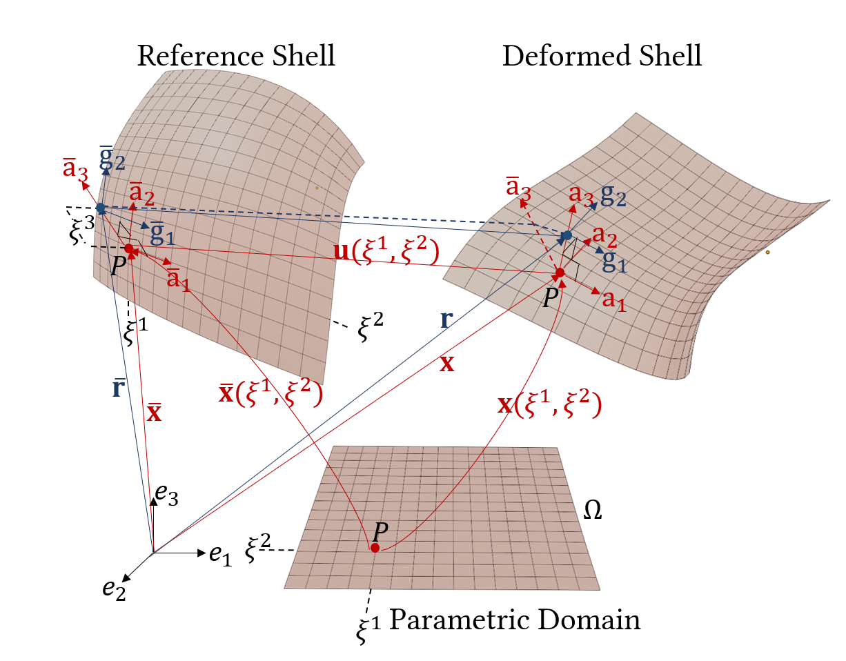
The Kirchhoff-Love model proposes a reduced kinematic parameterisation of a thin shell characterised by a 2D midsurface and shell director. It relies on the Kirchhoff hypothesis, i.e., the director initially perpendicular to the midsurface remains straight and normal, and the shell thickness $h\in\mathbb{R}$ does not change with deformation.

The position vector $\mathbf{\bar{r}}$ of a material point in the reference configuration of the shell continuum can be parametrised with curvilinear coordinates $(\xi^{1},\xi^{2})$ and thickness coordinate $\xi^{3}$ as:

(8) $$\mathbf{\bar{r}}(\xi^{1},\xi^{2},\xi^{3})=\mathbf{\bar{x}}(\xi^{1},\xi^{2})+\xi^{3}\mathbf{\bar{a}_{3}}(\xi^{1},\xi^{2}),\;\text{s.t.}\; -\frac{h}{2}\leq\xi^{3}\leq\frac{h}{2},$$

where $\mathbf{\bar{x}}(\xi^{1},\xi^{2})$ represents the midsurface.

Under the action of applied forces $\mathbf{f}$, the shell adopts a deformed configuration. Analogously, the deformed position vector $\mathbf{r}$ is represented as

(9) $$\mathbf{r}(\xi^{1},\xi^{2},\xi^{3})=\mathbf{x}(\xi^{1},\xi^{2})+\xi^{3}\mathbf{a}_{3}(\xi^{1},\xi^{2}),\;\text{s.t.}\; -\frac{h}{2}\leq\xi^{3}\leq\frac{h}{2},$$

where the deformed director $\mathbf{a}_{3}$ coincides with the unit normal.

As a consequence, the overall deformation of the Kirchhoff-Love shell is fully described by the displacement field $\mathbf{u}(\xi^{1},\xi^{2})$ of the midsurface, i.e.,

(10) $$\mathbf{x}(\xi^{1},\xi^{2})=\mathbf{\bar{x}}(\xi^{1},\xi^{2})+\mathbf{u}(\xi^{1},\xi^{2}).$$

The tangent base vectors at a point on the shell continuum are denoted by $\mathbf{g}_{i}:=\mathbf{r,}_{i}$ and expressed by those of the midsurface as:

(11) $$\begin{split}\mathbf{g}_{\alpha}&=\mathbf{a}_{\alpha}+\xi^{3}\mathbf{a}_{3,\alpha},\\ \mathbf{g}_{3}&=\mathbf{a}_{3}.\end{split}$$

The corresponding covariant components of the metric tensor are then obtained using

(12) $$g_{ij}:=\mathbf{g}_{i}\cdot\mathbf{g}_{j}.$$

To measure strain, we use the symmetric Green-Lagrange strain tensor $E_{ij}$, since it discards the rotational degrees of freedom from tangent base vector $\mathbf{g}_{i}$, while retaining the stretch and shear information. It is defined as the difference between the metric tensors on the deformed and undeformed configurations of the shell, i.e.,

(13) $$E_{ij}:=\frac{1}{2}(g_{ij}-\bar{g}_{ij}).$$

Using (11) and (12), note that transverse shear strain measuring the shearing of the director vanishes ($E_{\alpha 3}=0$) and the stretching of the director is identity, i.e., $E_{33}=1$; hence, the strain simplifies to

(14) $$E_{\alpha\beta}=\varepsilon_{\alpha\beta}+\xi^{3}\kappa_{\alpha\beta},$$

with membrane strain measuring the in-plane stretching defined as

(15) $$\varepsilon_{\alpha\beta}:=\frac{1}{2}(a_{\alpha\beta}-\bar{a}_{\alpha\beta}),$$

and bending strain measuring the change in curvature defined as

(16) $$\kappa_{\alpha\beta}:=\bar{b}_{\alpha\beta}-b_{\alpha\beta}.$$

3.4. Equilibrium Deformation

Under the action of external forces and boundary conditions, a thin shell deforms and achieves an equilibrium configuration. Its stable equilibrium state is characterised by the principle of minimum potential energy, a sum of external potential energy owing to applied forces and internal potential energy due to material elasticity. For simplicity, we use a linear isotropic stress-strain relationship leading to hyperelastic strain energy density (Simo and Fox, 1989) of the form

(17) $$\Psi=\frac{1}{2}(DH^{\alpha\beta\lambda\delta}\varepsilon_{\alpha\beta}\varepsilon_{\lambda\delta}+BH^{\alpha\beta\lambda\delta}\kappa_{\alpha\beta}\kappa_{\lambda\delta}),$$

where $D$ is the in-plane stiffness and $B$ is the bending stiffness computed as

(18) $$D:=\frac{Eh}{1-\nu^{2}}\;\text{and}\;B:=\frac{Eh^{3}}{12(1-\nu^{2})},$$

with Young’s modulus $E$, Poisson’s ratio $\nu$, and

(19) $$H^{\alpha\beta\lambda\delta}:=\nu\bar{a}^{\alpha\beta}\bar{a}^{\lambda\delta}+\frac{1}{2}(1-\nu)(\bar{a}^{\alpha\lambda}\bar{a}^{\beta\delta}+\bar{a}^{\alpha\delta}\bar{a}^{\beta\lambda}).$$

Here, $\Psi$ is the sum of the membrane strain energy density (the first term) and the bending strain energy density (the second term). Whereas all geometric quantities in (1)–(19) are defined at each material point $(\xi^{1},\xi^{2})\in\Omega$, the energy can be also integrated over the parametric domain. Considering the total potential energy of the shell $\mathcal{E}^{\mathrm{pot}}[\mathbf{u}]$ is given by the sum of elastic potential energy $\Psi$ and the potential energy due to the external force density $\mathbf{f}$, we obtain:

(20) $$\mathcal{E}^{\mathrm{pot}}[\mathbf{u}]=\int_{\Omega}\Psi\,d\Omega-\int_{\Omega}\mathbf{f}\cdot\mathbf{u}\,d\Omega.$$

Next, the stable equilibrium deformation of the shell can be found by minimising the potential energy functional subject to boundary constraints:

(21) $$\begin{split}&\mathbf{u^{*}}=\arg\min_{\mathbf{u}}\mathcal{E}^{\mathrm{pot}}[\mathbf{u}],\text{ subject to }\\ &\mathbf{u}(\xi^{1},\xi^{2})=\mathbf{b}(\xi^{1},\xi^{2})\text{ on }\partial\Omega.\end{split}$$

The above definition of hyperelastic energy of the shell requires the displacement field $\mathbf{u}\in H^{2}(\Omega\mapsto\mathbb{R}^{3})$ that must necessarily have square-integrable first and second derivatives.

Figure 3. Overview of the proposed NeuralClothSim. Our differentiable approach assumes a thin shell in the reference state along with boundary motion, its material properties and time-varying external forces as input. It learns a neural deformation field (NDF), i.e., a coordinate-based implicit 4D representation encoding surface evolution in the weights of a neural network. After the training (i.e., overfitting in a given simulation scenario), NDF can be queried using curvilinear-temporal coordinates for the state of the simulated surface continuously in space and time. The cloth dynamics is supervised by non-linear Kirchhoff-Love thin shell equations (a loss term based on its potential energy functional and kinetic energy for the dynamic case). In addition, NeuralClothSim can incorporate further priors learnt from data (e.g., it can be trained jointly with multiple materials).

4. Our Method for Cloth Simulation

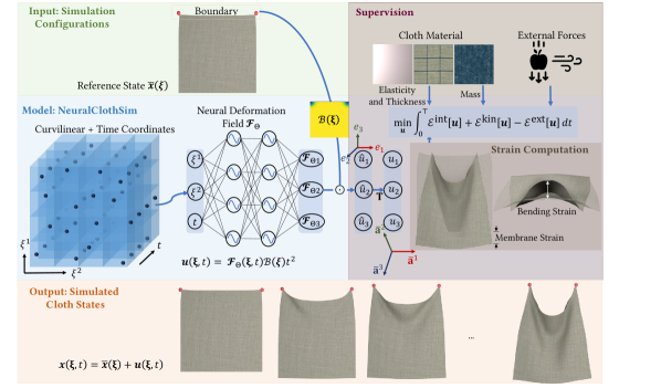
We propose NeuralClothSim, i.e., a new approach for dynamic cloth simulation relying on principles of thin shell theory. Given a cloth geometry in a reference configuration, its material properties, as well as time-varying external forces, our method automatically generates complex simulation states. The physical basis for our cloth dynamics is the non-linear Kirchhoff-Love thin shell equations that model the stretching and bending behaviour of cloths in a unified manner (see Sec. 3 for the preliminaries). We parameterise the cloth simulation states as a neural deformation field defined over a continuous spatio-temporal domain, described in Sec. 4.1. It explicitly accounts for boundary and initial conditions incorporating them as hard constraints (Sec. 4.2). To optimise for the neural deformation field, we define a loss function based on the Kirchhoff-Love potential energy functional, which is extended to the dynamic case by adding the kinetic energy (Sec. 4.3). Fig. 3 provides an overview of our method. To simulate various cloth materials without retraining, we extend our method to learn a prior over material space, presented in Sec. 4.4. Moreover, we present an approach to edit learned simulations when modifying the initial state or force conditions (Sec. 4.5). Note that we will continue to use the mathematical notations from the last section, with a few additions listed in Tab. 2.

4.1. Neural Deformation Field (NDF)

At the core of our approach is a neural deformation field (NDF), a continuous representation of cloth dynamics, entirely parameterised by a neural network. Following Sec. 3, we model cloth geometry as a Kirchhoff-Love thin shell. Given the rest state $\mathbf{\bar{x}}(\boldsymbol{\xi})$ of a cloth, we describe the time-varying simulated states $\mathbf{x}(\boldsymbol{\xi},t)$ of its midsurface under the action of external forces $\mathbf{f}(\boldsymbol{\xi},t)$ using

(22) $$\small\mathbf{x}(\boldsymbol{\xi},t)=\mathbf{\bar{x}}(\boldsymbol{\xi})+\mathbf{u}(\boldsymbol{\xi},t),\text{ with }\boldsymbol{\xi}:=(\xi^{1},\xi^{2})\in\Omega,\quad\forall t\in[0,T].$$

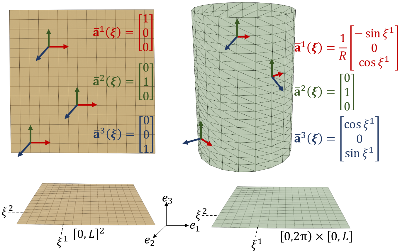
The curvilinear coordinate space $(\xi^{1},\xi^{2})$ can (but does not need to) naturally correspond to the orthotropic warp-weft structure of woven clothes. For example, the reference state associated with a flat square cloth in the $x$$y$-plane would be

(23) $$\mathbf{\bar{x}}(\boldsymbol{\xi})=[\xi^{1},\xi^{2},0]^{\top},\quad\forall(\xi^{1},\xi^{2})\in[0,L]^{2},$$

whereas the state of a garment sleeve admits a natural parameterisation with cylindrical coordinates:

(24) $$\mathbf{\bar{x}}(\boldsymbol{\xi})=[R\cos\xi^{1},\xi^{2},R\sin\xi^{1}]^{\top},\;\forall\xi^{1}\in[0,2\pi);\xi^{2}\in[0,L].$$

Analytically defining surface parameterisations might not be feasible for complex reference geometries. In such cases, we learn the reference parametrisation by overfitting a multilayer perceptron (MLP) $\mathbf{\bar{x}}(\boldsymbol{\xi};\Theta_{\mathrm{ref}})$ with parameters $\Theta_{\mathrm{ref}}$ to the reference mesh. It establishes a global parameterisation of the undeformed surface. Our key idea is to regress the spatio-temporal displacement field $\mathbf{u}(\boldsymbol{\xi},t)$ using an MLP $\mathcal{F}_{\Theta}:\Omega\times[0,T]\to\mathbb{R}^{3}$ and optimise its weights $\Theta$ to minimise the total mechanical energy of the thin-shell cloth. Specifically, the displacement field MLP is formulated as follows:

(25) $$\mathbf{u}(\boldsymbol{\xi},t;\Theta)=\mathcal{F}_{\Theta}(\boldsymbol{\xi},t)\mathcal{I}(t)\mathcal{B}(\boldsymbol{\xi}),$$

where $\mathcal{I}(t),\mathcal{B}(\boldsymbol{\xi})$ are scalar-valued functions that respectively account for initial and boundary conditions. In Sec. 4.2, we elaborate on the encoding of such conditions as hard constraints. While it is possible to predict final absolute 3D locations instead of displacements, we prefer the latter due to the following reasons. First, the prediction of zero displacement at the start of the simulation naturally corresponds to the initial rest state, constrained boundary and zero external force conditions. Second, the prior knowledge of shell geometry can be leveraged for faster optimisation, especially when they are complex (e.g., many garment types). Thus, the initial guess for $\mathbf{x}(\boldsymbol{\xi},t)$ prior to training is the sum of reference geometry $\mathbf{\bar{x}}(\boldsymbol{\xi})$ and the noisy displacements from the NDF.

Apart from being parameter-differentiable, i.e., the gradient $\nabla_{\Theta}\mathcal{F}_{\Theta}$ is defined everywhere, $\mathcal{F}_{\Theta}$ needs to be input-differentiable, i.e., $\nabla^{2}_{\boldsymbol{\xi}}\mathcal{F}_{\Theta}$ and $\nabla_{t}\mathcal{F}_{\Theta}$ must exist likewise, in order to compute the displacement and time derivatives required for the Kirchhoff-Love energy functional. This places restrictions on the activation function used in the network; only smooth non-linearities (such as GELU, softplus, sine or tanh) can be used. Furthermore, neural networks are biased towards learning low-frequency functions and we require an architecture that ensures the generation of high-frequency deformations such as folds and wrinkles. Therefore, we use periodic sine as the preferred activation function (Sitzmann et al., 2020) as it can represent high-frequency signals while allowing for computing higher-order derivatives. Sec. 4.3 describes the optimisation procedure to train the deformation field $\mathbf{u}(\boldsymbol{\xi},t;\Theta)$.

Once trained, $\mathcal{F}_{\Theta}$ provides implicit access to the continuous cloth dynamics, where the network can be consistently queried at any point and at varied resolutions. Based on the requirement of downstream applications, spatio-temporal input samples during inference can be different from those during training; see Fig. 1. Meshing and texture mapping can be achieved in the parametric domain and lifted from 2D to 3D using $\mathbf{u}(\boldsymbol{\xi},t;\Theta)$.

4.2. Initial and Boundary Conditions

Figure 4. Dirichlet and periodic boundary conditions. Although NeuralClothSim is trained with thin shell energy as the loss function (i.e., the physics-based constraints are soft), we strictly impose the user-specified boundary conditions (top row) as hard constraints. First, we formulate spatio-temporal functions encoding distance from the boundary— middle row visualises the scalar distance function in the parametric domain—and directly apply them to the NDF in bottom row-(a). For geometry parameterisations such as a sleeve, periodicity in the predictions can be enforced by rewriting NDF using the sine-cosine form of its Fourier series. In contrast to Dirichlet conditions that alter the network output, we impose periodic boundaries by remapping the network input parameter to its sine and cosine values, which is shown in bottom row-(b).

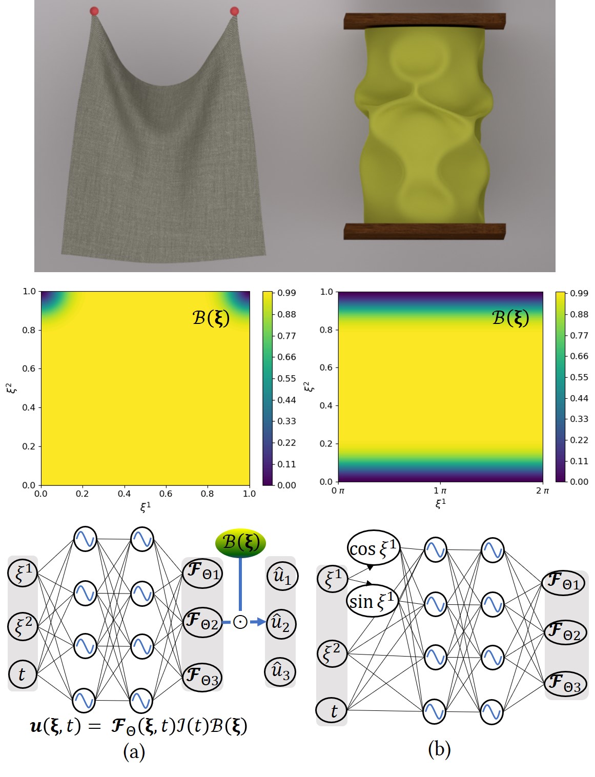
A practical cloth simulator allows for imposing conditions such as an initial rest state and a user-specified corner motion. For most garments, the simulation needs to be continuous and consistent along the seams, which can be modelled by imposing the periodicity constraint along a curvilinear coordinate (such as the azimuthal angle of a cylindrically parameterised sleeve). We seek to strictly enforce these conditions in NeuralClothSim. One way to achieve this would be to formulate boundary conditions as spatial and temporal distance functions and directly apply them to the NDF in (25). Then, the constraints are implicit during optimisation as we train for a deformation field respecting them. We next discuss Dirichlet, initial and periodic boundary conditions; see Fig. 4 for an overview.

4.2.1. Dirichlet Boundary Conditions

To constrain boundary positions, we require $\mathbf{u}(\boldsymbol{\xi}_{\partial\Omega},t)=\mathbf{0}$ for some specified list of parameter space points $\boldsymbol{\xi}_{\partial\Omega}$ along the boundary segment $\partial\Omega$. While we elaborate on the simpler case here, it is also possible to specify complex conditions i.e., $\mathbf{u}(\boldsymbol{\xi}_{\partial\Omega},t)=\mathbf{b}(\boldsymbol{\xi}_{\partial\Omega},t)$, detailed in Appendix. One solution is to sample points in the boundary segment and enforce the boundary conditions through separate loss terms. As shown in previous physics-informed neural networks (Hao et al., 2022), having competing objectives during training can lead to unbalanced gradients, which causes the network to often struggle with accurately learning the underlying solution. Further, there is no guarantee that the boundary conditions are always enforced. Therefore, we propose to modify the NDF to embed essential boundary conditions as hard constraints. Specifically, a distance function $\mathcal{B}(\boldsymbol{\xi})$ satisfying

(26) $$\mathcal{B}(\boldsymbol{\xi})=\begin{cases}0,\text{ if }\boldsymbol{\xi}\in\partial\Omega\\ {>}0,\text{ otherwise if }\boldsymbol{\xi}\in\Omega\end{cases}$$

ensures that any instance of deformation field $\mathbf{u}(\boldsymbol{\xi},t;\Theta)$ automatically satisfies the boundary conditions. We set

(27) $$\begin{split}\mathcal{B}(\xi^{1},\xi^{2}):=1-e^{-((\xi^{1}-\xi_{\partial\Omega}^{1})^{2}+(\xi^{2}-\xi_{\partial\Omega}^{2})^{2})/\sigma}\\ \text{s.t. }(\xi_{\partial\Omega}^{1},\xi_{\partial\Omega}^{2})\in\partial\Omega,\quad\forall(\xi^{1},\xi^{2})\in\Omega\end{split}$$

as a distance function with small support $\sigma$.

4.2.2. Initial Cloth Configuration

Consider the simulation starts from an initial rest state of the cloth, given beforehand as $\mathbf{\bar{x}}(\boldsymbol{\xi})$. Compared to mainstream cloth simulators that rely on incremental integration, our setting proposes global optimisation of a neural displacement field. Therefore, initial conditions need to be explicitly incorporated, as otherwise, the MLP will learn arbitrary initial displacement and velocity. Following the argument in setting up boundary conditions, we use the distance function

(28) $$\mathcal{I}(t):=t^{2}.$$

With substitution in (25), one can verify that it leads to

(29) $$\begin{split}\mathbf{u}(\boldsymbol{\xi},0)&=\mathbf{0},\;\text{and}\\ \dot{\mathbf{u}}(\boldsymbol{\xi},0)&=\mathbf{0}.\end{split}$$

4.2.3. Periodic Boundary Conditions

In contrast to the positional or motion-dependent boundary conditions specified as per user’s desires, additional boundary conditions can arise from the geometric cloth parametrisation. Typically, garments are formed by cutout panels that are joined together at the seams. Points along the panel seams share the world-space position and velocity, though they are mapped to different values in the parametric domain. We express continuity in geometry and simulation using periodic conditions. Consider any simulation involving a sleeve: In this case, our method needs to guarantee the additional condition due to the parametrisation, i.e., $\mathbf{u}(\xi^{1},\xi^{2},t)=\mathbf{u}(\xi^{1}\pm 2n\pi,\xi^{2},t)$. Similarly to the aforementioned spatio-temporal boundary conditions, we seek to strictly impose the periodic boundaries and do so by modifying the network architecture. Whereas the Dirichlet and initial conditions were imposed by altering the network output, we impose periodic boundaries by modifying the network input. Towards this, we first notice that any continuous periodic function can be written using its Fourier series. If $\mathbf{u}(\boldsymbol{\xi},t)$ is a periodic deformation field with period $P$ with respect to the input coordinate $\xi^{\lambda}$, $\mathbf{u}(\boldsymbol{\xi},t)$ can be decomposed into a weighted sum of the sines and cosines, i.e.,

$$\left\{1,\cos\left(\frac{2\pi\xi^{\lambda}}{P}\right),\sin\left(\frac{2\pi\xi^{\lambda}}{P}\right),\cos\left(\frac{4\pi\xi^{\lambda}}{P}\right),\sin\left(\frac{4\pi\xi^{\lambda}}{P}\right),...\right\}.$$

Due to the universal approximation power of MLP, only the first cosine and sine terms need to be considered, as the others can be expressed as the nonlinear continuous functions of $\cos\left(\frac{2\pi\xi^{\lambda}}{P}\right)$ and $\sin\left(\frac{2\pi\xi^{\lambda}}{P}\right)$ (Lu et al., 2021). Therefore, we map the network input coordinate using $\xi^{\lambda}\mapsto\left\{\cos\left(\frac{2\pi\xi^{\lambda}}{P}\right),\sin\left(\frac{2\pi\xi^{\lambda}}{P}\right)\right\}$ when feeding it to the MLP, enforcing periodicity of the predicted NDF along $\xi^{\lambda}$.

This completes the definition of spatial and temporal boundary conditions, which can be directly integrated into our NDF $\mathbf{u}(\boldsymbol{\xi},t;\Theta)$. Note that the constraints are applied at, both, training and inference.

4.3. NDF Optimisation

Figure 5. Contravariant basis for thin shells in the reference configuration. While a local contravariant basis coincides with the global Cartesian coordinate system for a planar reference shell, such a basis varies in magnitude and direction across any circular section of the cylinder. Local basis relies on the surface parameterisation, therefore the derived basis vectors need not be normalised (notice how $\bar{\mathbf{a}}^{1}(\boldsymbol{\xi})$ scales inversely with the radius). Thus, the Cartesian coordinate system is better suited for NDF training.

Previous sections described modelling of cloths using an NDF with (optional) boundary and initial conditions. We next proceed with an optimisation strategy for learning such an NDF. For notational clarity, we drop the function arguments $(\boldsymbol{\xi},t)$ for $\mathbf{u}(\boldsymbol{\xi},t)$ and quantities derived from it.

4.3.1. Strain Calculation

To compute the geometric strains due to the thin shell deformation, we evaluate the NDF on samples from the curvilinear coordinate space $\Omega$ and the time domain $[0,T]$. We generate $N_{\Omega},N_{t}$ points using a stratified sampling approach. This ensures that the samples are random, yet well-distributed. At each training iteration, we re-sample coordinates from the parametric and temporal space to learn an NDF that fully explores the continuous domain over the course of the optimisation. We evaluate NDF $\mathbf{u}(\boldsymbol{\xi},t)$ at all samples using (25) and this prediction is assumed to be in a Cartesian coordinate system, i.e., $\mathbf{u}=\hat{u}_{i}\mathbf{e_{i}}$. Although our further strain computations require covariant components of local contravariant basis, i.e., $\mathbf{u}=u_{\alpha}\mathbf{\bar{a}}^{\alpha}+u_{3}\mathbf{\bar{a}}^{3}$, prediction in a global frame is better suited for NDF training, as shown in Fig. 5. This is expected as the local basis vectors are not normalised and the basis varies with the input position $\boldsymbol{\xi}$, especially noticeable for reference geometries such as the ones described in (24). Here, the basis transformation matrix $\mathbf{T}=[\mathbf{\bar{a}}^{1}\ \mathbf{\bar{a}}^{2}\ \mathbf{\bar{a}}^{3}]^{-1}$ is used for converting the displacement from Cartesian coordinates to covariant coordinates.

Next, we describe the ingredients required to evaluate the internal strain energy $\Psi$. While membrane and bending strains can be obtained with (15) and (16) using the reference $\mathbf{\bar{x}}$ and deformed midsurface $\mathbf{x}=\mathbf{\bar{x}}+\mathbf{u}$, we simplify these equations to directly operate on $\mathbf{u}$. With the assumptions of Kirchhoff-Love theory and following (Basar and Krätzig, 2013), membrane strain $\boldsymbol{\varepsilon}$ and bending strain $\boldsymbol{\kappa}$ are evaluated as

(30) $$\begin{split}\varepsilon_{\alpha\beta}&=\frac{1}{2}(\varphi_{\alpha\beta}+\varphi_{\beta\alpha}+\underbrace{\varphi_{\alpha\lambda}\varphi_{\beta}^{\lambda}+\varphi_{\alpha 3}\varphi_{\beta 3}}_{\text{non-linear}}),\\ \kappa_{\alpha\beta}&=-\varphi_{\alpha 3}|_{\beta}-\bar{b}_{\beta}^{\lambda}\varphi_{\alpha\lambda}+\underbrace{\varphi^{\lambda}_{3}(\varphi_{\alpha\lambda}|_{\beta}+\frac{1}{2}\bar{b}_{\alpha\beta}\varphi_{\lambda 3}-\bar{b}_{\beta\lambda}\varphi_{\alpha 3}}_{\text{non-linear}}),\end{split}$$

where the deformation gradients $\varphi_{\alpha\lambda},\varphi_{\alpha 3}$ are the components of $\mathbf{u}_{,\alpha}$ such that

(31) $$\begin{split}\mathbf{u}_{,\alpha}&=\varphi_{\alpha\lambda}\mathbf{\bar{a}}^{\lambda}+\varphi_{\alpha 3}\mathbf{\bar{a}}^{3},\\ \varphi_{\alpha\lambda}&:=u_{\lambda}|_{\alpha}-\bar{b}_{\alpha\lambda}u_{3},\\ \varphi_{\alpha 3}&:=u_{3,\alpha}+\bar{b}_{\alpha}^{\lambda}u_{\lambda}.\end{split}$$

We refer the reader to Appendix C for the proof of the above expressions for strain. Note that we do not linearise the strain components, while some earlier works (Thomaszewski et al., 2006) use corotational strain formulation to benefit from the convergence properties of a linear approach. Next, we discuss how we optimise the total energy of the system.

4.3.2. Energy Optimisation

We extend the equilibrium deformation of the Kirchhoff-Love thin shell from quasi-static to the dynamic case with the addition of kinetic energy:

(32) $$\mathcal{E}^{\mathrm{kin}}[\mathbf{u}] =\frac{1}{2}\int_{\Omega}\rho|\dot{\mathbf{u}}|^{2}\,d\Omega,$$

(33) $$\mathcal{E}[\mathbf{u}] =\int_{0}^{\top}\mathcal{E}^{\mathrm{pot}}[\mathbf{u}]+\mathcal{E}^{\mathrm{kin}}[\mathbf{u}]\,dt.$$

Following the variational formulation of (Thomaszewski et al., 2006) and (Lu and Zheng, 2014), the total mechanical energy of the dynamic system must be at a minimum for attaining the dynamic equilibrium configurations:

(34) $$\mathbf{u^{*}} =\arg\min_{\mathbf{u}}\mathcal{E}[\mathbf{u}].$$

In earlier Kirchhoff-Love theory-based simulators operating on meshes (Thomaszewski et al., 2006; Clyde et al., 2017), the first variation of the energy is set to zero. Specifically, the Euler-Lagrange equations in weak form, i.e., $\delta\mathcal{E}[\mathbf{u};\delta\mathbf{u}]=0$, are solved for the optimality condition. Alternatively, we take advantage of the variational structure of the total energy and minimise it directly using gradient descent. As shown in other works (Bastek and Kochmann, 2023), employing energy as the loss—instead of solving Euler-Lagrange equations—is advantageous in two ways: It does not increase the order of derivatives and it automatically incorporates the natural boundary conditions. All operations of our energy computation are naturally differentiable and we estimate the integral using the Monte-Carlo method optimising over continuous parametric and time domains. Finally, we minimise the following loss function to optimise the MLP weights for a physically-principled cloth simulation encoded as $\mathbf{u}^{*}(\boldsymbol{\xi},t;\Theta)$:

(35) $$\mathcal{L}(\Theta) =\frac{|\Omega|}{N_{\Omega}N_{t}}\sum_{i=1}^{N_{\Omega}}\sum_{j=1}^{N_{t}}\Big{(}\frac{1}{2}\underbrace{D\boldsymbol{\varepsilon}^{\top}(\boldsymbol{\xi}_{i},t_{j};\Theta)\mathbf{H}(\boldsymbol{\xi}_{i})\boldsymbol{\varepsilon}(\boldsymbol{\xi}_{i},t_{j};\Theta)}_{\text{membrane energy}}+$$

$$+\frac{1}{2}\underbrace{B\boldsymbol{\kappa}^{\top}(\boldsymbol{\xi}_{i},t_{j};\Theta)\mathbf{H}(\boldsymbol{\xi}_{i})\boldsymbol{\kappa}(\boldsymbol{\xi}_{i},t_{j};\Theta)}_{\text{bending energy}}-$$

$$-\underbrace{\mathbf{f}^{\top}(\boldsymbol{\xi}_{i},t_{j})\mathbf{u}(\boldsymbol{\xi}_{i},t_{j};\Theta)}_{\text{external energy}}+\frac{1}{2}\underbrace{\rho|\dot{\mathbf{u}}(\boldsymbol{\xi}_{i},t_{j};\Theta)|^{2}}_{\text{kinetic energy}}\Big{)}\sqrt{\bar{a}(\boldsymbol{\xi}_{i})},$$

where $\boldsymbol{\varepsilon}(\boldsymbol{\xi},t)\in\mathbb{R}^{4}$, $\boldsymbol{\kappa}(\boldsymbol{\xi},t)\in\mathbb{R}^{4}$ are strains computed using (30); $|\Omega|=\int_{\Omega}\,d\xi^{1}d\xi^{2}$ is the area of the parametric domain; $\mathbf{H}(\boldsymbol{\xi})\in\mathbb{R}^{4\times 4}$ is computed using (19) and depends only on the reference surface. The external force $\mathbf{f}$ is expressed as contravariant components $\mathbf{f}=f^{\alpha}\mathbf{\bar{a}}_{\alpha}+f^{3}\mathbf{\bar{a}}_{3}$ to compute the inner product with $\mathbf{u}=u_{\alpha}\mathbf{\bar{a}}^{\alpha}+u_{3}\mathbf{\bar{a}}^{3}$.

To accurately evaluate the derivatives of all physical and geometric quantities with respect to input parameters $\boldsymbol{\xi},t$, we use automatic differentiation of modern machine learning frameworks (Paszke et al., 2019). However, care must be taken so that the gradient back-propagation during optimisation should be enabled only for quantities dependent on the NDF.

4.4. Material-conditioned NDFs

We next show that NeuralClothSim can also incorporate learnt priors: Our NDF can be directly extended by making it dependent on the material properties, i.e., it can accept the material parameters as an extra input. This is possible since the material parameters space is typically low-dimensional. Once such NeuralClothSim modification is trained, we can edit the simulated geometry at test time.

We first define the set of material parameters as

(36) $$\boldsymbol{\Phi}:=\{\rho,h,E,\nu\}.$$

Conditioning on $\boldsymbol{\Phi}$ allows us adjusting at test time mass density $\rho$, cloth thickness $h$, as well as the linear isotropic elastic properties of the material, i.e., Young’s modulus $E$ and the Poisson’s ratio $\nu$. The updated NDF—which is now a function of material as well—reads:

(37) $$\mathbf{u}(\boldsymbol{\xi},t,\boldsymbol{\Phi};\Theta)=\mathcal{F}_{\Theta}(\boldsymbol{\xi},t,\boldsymbol{\Phi})\mathcal{I}(t)\mathcal{B}(\boldsymbol{\xi}),$$

where $\boldsymbol{\Phi}\in[\boldsymbol{\Phi}_{\mathrm{min}},\boldsymbol{\Phi}_{\mathrm{max}}]$ is the continuous range of material parameters. At each training iteration, we uniformly (at random) re-sample $\boldsymbol{\Phi}$ to explore the entire material domain. Finally, the updated loss function reads:

(38) $$\mathcal{L}(\Theta) =\frac{|\Omega|}{N_{\Omega}N_{t}}\sum_{i=1}^{N_{\Omega}}\sum_{j=1}^{N_{t}}\Big{(}\frac{1}{2}\frac{Eh}{1-\nu^{2}}\boldsymbol{\varepsilon}^{\top}(\boldsymbol{\xi}_{i},t_{j},\boldsymbol{\Phi};\Theta)\mathbf{H}(\boldsymbol{\xi}_{i},\nu)\boldsymbol{\varepsilon}(\boldsymbol{\xi}_{i},t_{j},\boldsymbol{\Phi};\Theta)+$$

$$+\frac{1}{2}\frac{Eh^{3}}{12(1-\nu^{2})}\boldsymbol{\kappa}^{\top}(\boldsymbol{\xi}_{i},t_{j},\boldsymbol{\Phi};\Theta)\mathbf{H}(\boldsymbol{\xi}_{i},\nu)\boldsymbol{\kappa}(\boldsymbol{\xi}_{i},t_{j},\boldsymbol{\Phi};\Theta)-$$

$$-\mathbf{f}^{\top}(\boldsymbol{\xi}_{i},t_{j})\mathbf{u}(\boldsymbol{\xi}_{i},t_{j},\boldsymbol{\Phi};\Theta)+\frac{1}{2}\rho|\dot{\mathbf{u}}(\boldsymbol{\xi}_{i},t_{j},\boldsymbol{\Phi};\Theta)|^{2}\Big{)}\sqrt{\bar{a}(\boldsymbol{\xi}_{i})}.$$

At test time, novel simulation can be generated with a single forward pass for any material $\boldsymbol{\Phi}$ in the valid material range $[\boldsymbol{\Phi}_{\mathrm{min}},\boldsymbol{\Phi}_{\mathrm{max}}]$.

To summarise, apart from the possibility to query the NDF continuously in space and time, our method can also linearly interpolate in the material space. Moreover, unlike latent space conditioning in other fields and problems, the material space conditioning in NeuralClothSim has a direct physical (semantic) interpretation.

4.5. NDF Editing

In movie and game production, a 3D artist’s workflow includes updating design parameters requiring multiple repeated simulations from scratch. Such scene parameters include reference state geometry, external forces, and material properties. Material parameters typically constitute a low dimensional space and, therefore, we propose to condition the NDF on material properties. However, other inputs such as shape and pose of reference state, and external force are high-dimensional. Instead of learning simulations over the entire scene space, we offer simulation editing the following way: the user can interrupt the training of NDF at any point, change the scene parameters and continue training for successive improvement. On the other hand, editing can also be done after full convergence (aka pre-training) and then fine-tuning with gradually modified design parameters. Editing a NDF provides multiple advantages over training a new NDF from scratch: It is computationally and memory efficient, and provides access to interpolated simulations.

In the following, we demonstrate editing of the following scene parameters: (a) external force, and (b) reference state geometry. The key idea is to use the modified scene parameters in the loss function and update the NDF weights with gradient-based optimisation. Specifically, given a cloth geometry $\mathbf{\bar{x}}$, external forces $\mathbf{f}$, we train an NDF to obtain a simulation $\mathbf{u}^{*}$ parameterised by network weights $\Theta^{*}$, as described in the main method. As an editing objective, we would like to arrive at a novel simulation corresponding to external force $\mathbf{f}^{I}$ and/or reference geometry $\mathbf{\bar{x}}^{I}$ with $I\in\mathbb{N}$ training iterations. Here, $I$ is much smaller than the iterations needed for the convergence of the original simulation. We can then fine-tune the pre-trained NDF over iterations $i\in\{0,...,I\}$ by minimising the loss function, $\mathcal{L}(\Theta;\mathbf{f}^{i},\mathbf{\bar{x}}^{i})$ to obtain edited and interpolated simulations $\mathbf{u}^{i},\Theta^{i}$. Here, we assume a smooth transition of external force or the reference shape from the initial to the edited value, which can be obtained, for example, by linear interpolation, i.e., $\mathbf{f}^{i}=\operatorname{lerp}(\mathbf{f},\mathbf{f}^{I},\frac{i}{I})$.

5. Experimental Evaluation

This section validates our formulation of the first cloth simulator operating on continuous neural fields. We present qualitative results and highlight the new characteristics that mesh-based approaches currently lack. Recall that cloth simulation is a challenging problem that does not have a general analytical solution. Due to the numerical approximations and simplifications of the underlying physics and the material model of the cloth, works in this field do not provide a comparison to ground truth, and focus rather on realism over accuracy. Moreover, recent works improve various aspects of usability of the approaches, such as fast GPU implementation (Wang, 2021), simulation of wrinkles at very high resolution (Li et al., 2020), and making the simulators differentiable (Liang et al., 2019; Li et al., 2022) for inverse problems.

We next present our experimental setup, the qualitative and empirical results. We first show validation results (Sec. 5.1), such as the Belytschko obstacle course for thin shells. We then follow with qualitative results (Sec. 5.2) and afterwards compare NeuralClothSim to several existing cloth simulators (Sec. 5.3). Next, we conduct an ablative study (Sec. 5.4) and, finally, demonstrate several applications of the proposed technique (Sec. 5.5). More evaluations of the performance (including runtime and scalability to longer simulations) and robustness are provided in Appendices G and H.

5.1. Obstacle Course

Figure 6. Belytschko obstacle course. We consider the following benchmark problems (Belytschko et al., 1985; Timoshenko et al., 1959): (a) Square plate (b) Scordelis-lo Roof, (c) pinched cylinder with rigid diaphragms, and (d) pinched cylinder with free boundaries. The quasi-static version of our method generates accurate and converged NDF for these test cases. Top row: Reference geometries; bottom: deformed geometries. For better visualisation of each experimental result, the computed displacement fields (NDF) are scaled up by a factor of 50, 10, 80, and 5, respectively.

Table 3. Numerical evaluation on an obstacle course. We validate the maximum displacements obtained with our method on the Belytschko obstacle course with analytical solutions from (Belytschko et al., 1985; Timoshenko et al., 1959). The Scordelis-Lo roof result is compared with (Bastek and Kochmann, 2023) and the square plate result is compared with (Guo et al., 2021) (“n/a” denotes that a method does not support the corresponding example). Note that their material parameters are different, and they report a maximum displacement of $2.56654$ (closely matches with the analytical displacement of $2.56649$ in their case). In the second part (two bottom rows), we show ablation of our method when 1) removing periodic boundary constraint on the cylindrical shell, and 2) using GELU instead of sine activation.

Method	Square plate	Scordelis-Lo roof	Pinched cylinder (rigid ends)	Pinched cylinder (free ends)
Analytical	0.487	0.3024	$1.82510-5$	$4.5210-4$
Guo et al.	2.566*	n/a	n/a	n/a
Bastek et al.	n/a	0.297	n/a	n/a
Ours, full	0.487	0.3018	$1.8110-5$	$4.5810-4$
Ours, no periodicity	n/a	n/a	$3.610-9$	$3.1310-6$
Ours, GELU	0.496	0.288	$1.7410-5$	$5.710-4$

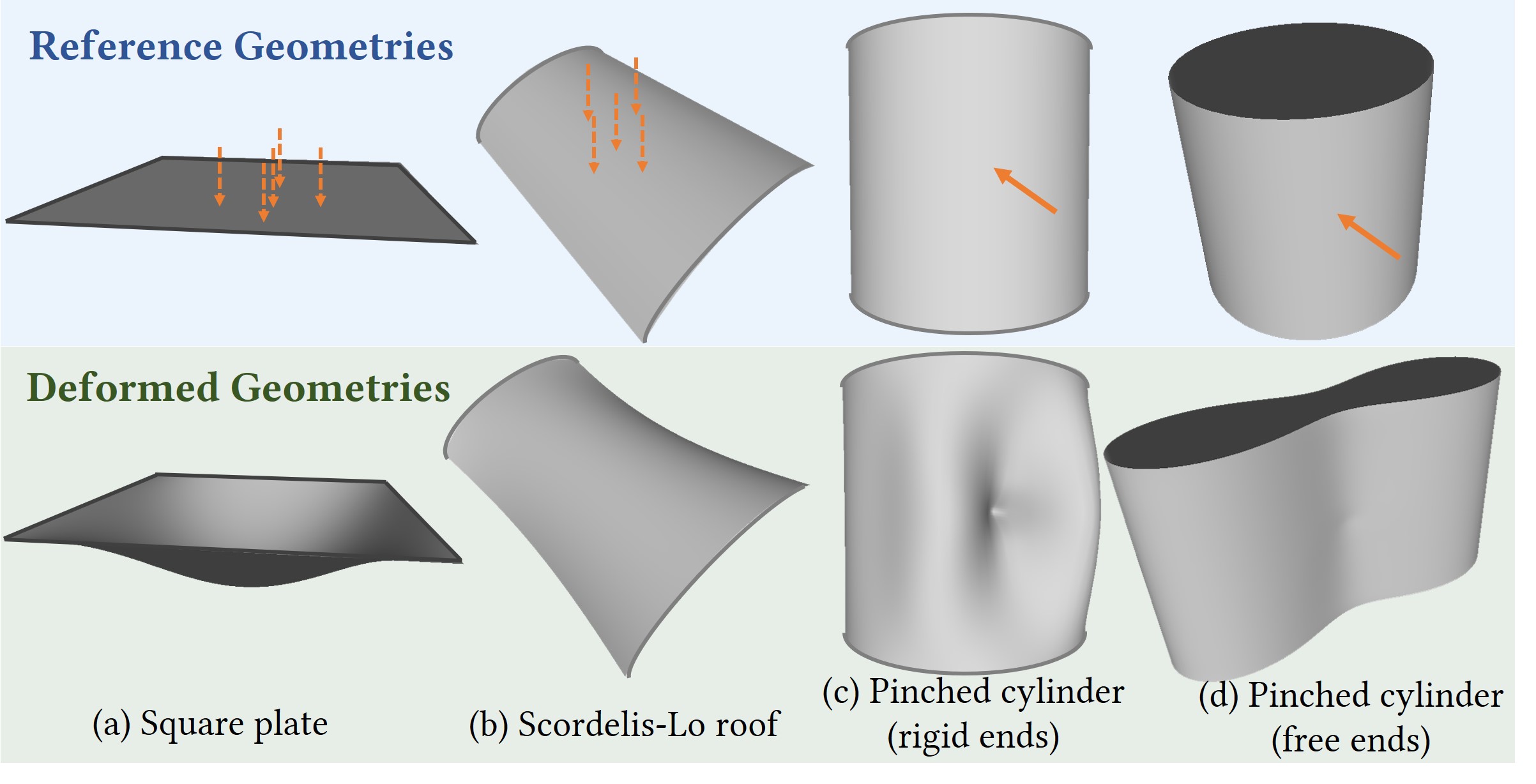
We first validate how our approach reproduces quasi-static deformations of thin shells. We use the engineering obstacle course of benchmark problems from Belytschko et al. (1985), for which the analytical solutions are known for linearised functionals. Such problems were previously used in computer graphics (Grinspun et al., 2006) for testing the performance and accuracy of finite mesh elements. Specifically, we test the performance of our method on square plate (Timoshenko et al., 1959), the Scordelis-Lo roof, and the pinched cylinder (Belytschko et al., 1985) examples, for which the original and deformed shells (results of our method) are shown in Fig. 6. Converged numerical results are compared with reference values in Tab. 3. We present the detailed experimental setup including the precise form of geometry, boundary conditions as well as loss functions in Appendix D, including visualisations of the full displacement fields.

Square Plate. In the first test case, we consider a simple bending problem of a flat square shell (Cirak et al., 2000). It is simply supported at all edges and is subject to a uniform load. The plate has a side length of $L=\qty{100}{}$ and a thickness $h=\qty{1}{}$ and, therefore, falls under the scope of Kirchhoff-Love thin shell theory. The material parameters are given as $E=\qty{1e7}{}$ and $\nu=0$. We represent the reference geometry with (23) and impose Dirichlet boundary constraints by constructing a distance function to the plate edges. This is followed by training an NDF to solve for quasi-static displacement minimising the total potential energy (20) subject to external load $\mathbf{f}=[0,0,-1]^{\top}$. We train for 2500 iterations and illustrate the solution in Fig. 6 where the displacement is scaled up by a factor of $50$. The maximum displacement $u_{3}$ at the centre of the plate is found to be 0.487 after convergence and exactly matches the reference solution (Timoshenko et al., 1959).

Scordelis-Lo Roof. Next, we consider Scordelis-Lo Roof (Scordelis and Lo, 1964), a non-flat reference shape subject to complex membrane strains. The roof is an open cylindrical shell with radius $R=\qty{25}{}$, length $L=\qty{50}{}$ and subtends an angle of $\qty{80}{}$. It is supported with two rigid diaphragms at the ends and loaded by gravity forces, $\mathbf{f}=[0,-90,0]^{\top}$. The shell’s material is given as $E=\qty{4.32e8}{},\nu=0$, whereas its thickness $h=\qty{0.25}{}$. Similar to the square plate, we solve for a static NDF. We obtain the maximum vertical displacement $u_{2}$ at the centre of the edge (averaged over the two sides) as $0.3018$, which closely approximates the reference solution $u_{2}=0.3024$ (Belytschko et al., 1985).

Pinched Cylinder. Finally, we consider the pinched cylinder problem, i.e., one of the most severe tests for both inextensional bending modes and complex membrane states. As shown in Fig. 6, a cylindrical shell is pinched with two diametrically opposite unit loads applied at the middle of the shell. We consider two cases: First, a shell with ends supported by rigid diaphragms (Belytschko et al., 1985) (similar to Scordelis-Lo roof), and second, a cylinder with free ends (Timoshenko et al., 1959). We define the cylinder geometry with (24), where $R=\qty{300}{},L=\qty{600}{}$ and the thickness is set to $h=\qty{3}{}$; the material properties are given as $E=\qty{3e6}{},\nu=0.3$. In contrast to the previous test geometries, which required specifying only the Dirichlet boundary conditions, we additionally model here the periodicity constraint along the circular cross-sections. A crucial challenge of this test case is modelling load at singular points in the sample space. To achieve this, we adapt the potential energy functional (20)—described previously for uniformly distributed forces —to the point load setting, rewriting it as

(39) $$\mathcal{E}^{\mathrm{pot}}[\mathbf{u}]=\int_{\Omega}\Psi\,d\Omega-\textstyle\sum_{\Omega_{0}}\mathbf{f}\cdot\mathbf{u},$$

where $\Omega_{0}=\{(\qty{90}{},300),(\qty{270}{},300)\}$ is the set of points of the load application. In the case of distributed load, we previously proposed the computation of external and hyperelastic strain energy at an identical set of stratified samples in the parametric domain. We depart from this setting for point loads: At each training iteration, we sample all points from $\Omega_{0}$ for external energy, whereas random stratified samples are used for computing strain energy. The exact loss function and training details are provided in Appendix D. To speed up the convergence, we set $E=\qty{30}{}$ instead of the original value $E=\qty{3e6}{}$; this simply scales the displacement field in the linear setting as shown in (Bastek and Kochmann, 2023).

Next, consider a pinched cylinder with free ends. Without any boundary constraints, the cylinder can move rigidly due to the applied force, and such rigid body motion should be factored out. Therefore, to suppress it, we restrict the displacement of the point under the load in directions other than the direction of the force vector. We achieve this by enforcing $\hat{u}_{1}=0,\hat{u}_{2}=0$ at load points. In both examples with a pinched cylinder, we monitor the displacements under the loading point. As shown in Fig. 6 and Tab. 3, it qualitatively and quantitatively converges to the reference solution.

A scrupulously modelled thin shell must have the ability to handle inextensional bending modes, complex membrane states of stress and rigid body motion without straining. The excellent modelling ability of our method is evident from the results.

5.2. Qualitative Results

In contrast to the previous quasi-static case, we next present the results of our full approach, where we model the dynamics and deformations of thin shells. The experiments are performed with the following default values unless specified otherwise: $E=\qty{5000}{},\nu=0.25,\rho=\qty{0.144}{\per\squared},h=\qty{0.0012}{}$, and $\sigma=0.01$. Details on boundary conditions, external forces and NDF (after incorporating the boundary constraints) can be found in Appendix E.

Napkin. We first consider a square napkin of length $L=\qty{1}{}$, falling freely under the effect of gravitational force. The napkin has a flat reference state in the xy-plane given by (23), and the gravitational force field is applied along the negative y-axis, i.e., external force density $\mathbf{f}=[0,-9.8\rho,0]^{\top}$. To constrain the napkin movement, we specify a fixed boundary condition at the top left corner. The simulation is run for $T=\qty{2}{}$. We train with (35) to learn the simulation; the meshes extracted from the trained NDF are visualised in Fig. 1-(bottom row, left and middle columns). Note that apart from its realism, one can also query the simulation at arbitrary resolution in the case of NeuralClothSim. Next, we perform another experiment with a napkin subject to gravity and dynamic boundary condition, i.e., in which the corners are moving inwards. This leads to fold formation at the top as visualised in Fig. 3-(bottom row).

Sleeve. We also consider a cylindrical shell and perform two experiments with sleeve compression and twisting applied by a user. In both cases, we consider the reference state (24) with $L=\qty{1}{}$ and $R=\qty{0.25}{}$ and simulate for $T=\qty{1}{}$. See Figs. 4-(b) and 9-(b) for visualisations of our two experiments with the sleeve. In the first case, we apply torsional motion on the sleeve, i.e., a total rotation of $\frac{3\pi}{4}$ around they-axis to both the top and bottom rims. The optimised NDF forms wrinkles at the centre as expected (Guo et al., 2018); please refer to the supplementary video for the full visualisation.

In the second example, we compress the sleeve to produce the characteristic buckling effect. We do not apply external forces here and the compression is entirely specified by boundary conditions. We achieve a total displacement of $\qty{0.2}{}$ due to compression with the time-dependent inward motion of the top and bottom rims along the cylinder axis; see Fig. 4-(right) for the compression result. The demonstrated simulation is a representative example of strain localisation, with noticeable diamond patterns of shell buckling.

5.3. Comparisons to Previous Methods

Figure 7. Comparison of simulation consistency of state-of-the-art differentiable simulators and our approach. At different discretisations of the initial state, FEM-based simulators (e.g., ARCSim (Liang et al., 2019) and DiffCloth (Li et al., 2022)) lead to inconsistent results with often occurring differences in the folds or wrinkles. In contrast, our NeuralClothSim overfits an MLP to the reference mesh and encodes the surface evolution using another MLP, both of which are continuous neural fields. This reduces the sensitivity of our method to spatial discretisations, leading to consistent simulations.

Figure 8. Evaluating the memory efficiency. We plot the memory requirements for simulations generated by NeuralClothSim and DiffARCSim (Liang et al., 2019), and DiffCloth (Li et al., 2022) as functions of (left:) spatial resolution (number of vertices), and (right:) temporal resolution (frame rate). The simulations are chosen to be of similar complexity and the same length and are visualised in Fig. IX-appendix. The constant memory requirement of our approach is due to the compressing property of the MLP weights that encode the simulations in our case. The memory requirement of other classical approaches grows linearly with the mesh resolution and frame rate, which can often become prohibitive.

In this section, we compare NeuralClothSim to state-of-the-art differentiable simulators (Liang et al., 2019; Li et al., 2022) and physics-informed neural networks for shell structures (Bastek and Kochmann, 2023). While there are other neural simulators like (Bertiche et al., 2022; Santesteban et al., 2022), we do not (and cannot) compare against them as their goal is high-level modelling of garments, whereas ours is general neural cloth simulation. First, they use skinned 3D body models and compute clothing deformations as a function of the body pose or motion. As they do not support simulating cloths not worn by humans or mannequins, they cannot be adapted to our setting. On the other hand, our method does not handle contacts and collisions yet. Note that previous neural methods use explicit mesh representation and finite time stepping, similar to FEM simulators (Narain et al., 2012).

Differentiable Cloth Simulators. The technique of Liang et al. (2019) is a differentiable version of ARCSim (Narain et al., 2012). ARCSim uses discretisation in space with FEM and integration in time using an implicit Euler approach. DiffCloth (Li et al., 2022) is a state-of-the-art differentiable cloth simulator based on Projective Dynamics (PD) (Ly et al., 2020). These simulators discretise the cloth surface as meshes and generate simulations at the mesh resolution of the initial state. They need to run from scratch for different mesh resolutions and the simulation behaviour is mesh-dependent. On the other hand, consistent simulation at different discretisations is a desirable method property for cloth simulation. Some cloth simulators use adaptive mesh refinement (Narain et al., 2012; Bender and Deul, 2012) to adjust the discretisation level according to the dynamic detail of the simulated cloth. While these do not suffer from inconsistency, they do not demonstrate differentiability, unlike the ones with a fixed number of vertices (Liang et al., 2019).

In the next experiment, we validate the consistency of cloth simulations at different discretisations of the reference state. We consider two evaluation scenarios: 1) A napkin with a fixed corner under gravity simulated with our approach and DiffARCSim (Li et al., 2022) (Fig. 7, left), and 2) a flag with two fixed corners deforming under wind and gravity simulated with our approach and DiffCloth (Li et al., 2022) (Fig. 7, right). In both scenarios, we simulate thrice starting with a marginally different meshing of the same initial geometry. While the compared FEM-based methods directly take the reference mesh as the input, our approach overfits an MLP to it, as described in Sec. 4.1. Specifically, we learn $\mathbf{\bar{x}}(\boldsymbol{\xi};\Theta_{\mathrm{ref}})$ by supervising with the $\ell_{2}$-loss $\mathcal{L}(\Theta_{\mathrm{ref}})=||\mathbf{\bar{x}}(\boldsymbol{\hat{\xi}};\Theta_{\mathrm{ref}})-\mathbf{\hat{\bar{x}}}||^{2}_{2}$, where $\mathbf{\hat{\bar{x}}}\in\mathbb{R}^{3},\boldsymbol{\hat{\xi}}\in\mathbb{R}^{2}$ are the vertices and texture coordinates of the given reference mesh. After the reference MLP is trained, we proceed with learning an NDF that encodes the cloth simulation. The advantage of this preprocessing over directly using reference mesh is that we can sample continuously in the parametric domain by querying the MLP and compute all the geometric quantities (such as metric and curvature tensors) at these points, similar to analytical access to the reference surface.

Note that unlike NDF $\mathbf{u}(\boldsymbol{\xi};\Theta)$, which uses periodic sine activation function to generate high-frequency folds, we use GELU (Hendrycks and Gimpel, 2016) activation for smoothly fitting the reference shape, $\mathbf{\bar{x}}(\boldsymbol{\xi};\Theta_{\mathrm{ref}})$. We observe that for competing methods, simulation is sensitive to the discretisation of the initial template: While multiple simulations with the same discrete initial state produce identical results, slightly different meshing generates simulated states that are inconsistent with each other. As seen in Fig. 7, they lead to different folds and wrinkles. We use the same mesh size (i.e., the number of vertices) across varying initialisation, to fairly compare the computational time and memory requirements. In contrast, meshes extracted from NDF produced by NeuralClothSim and, hence, the simulations, are consistent for different initial discretisations.

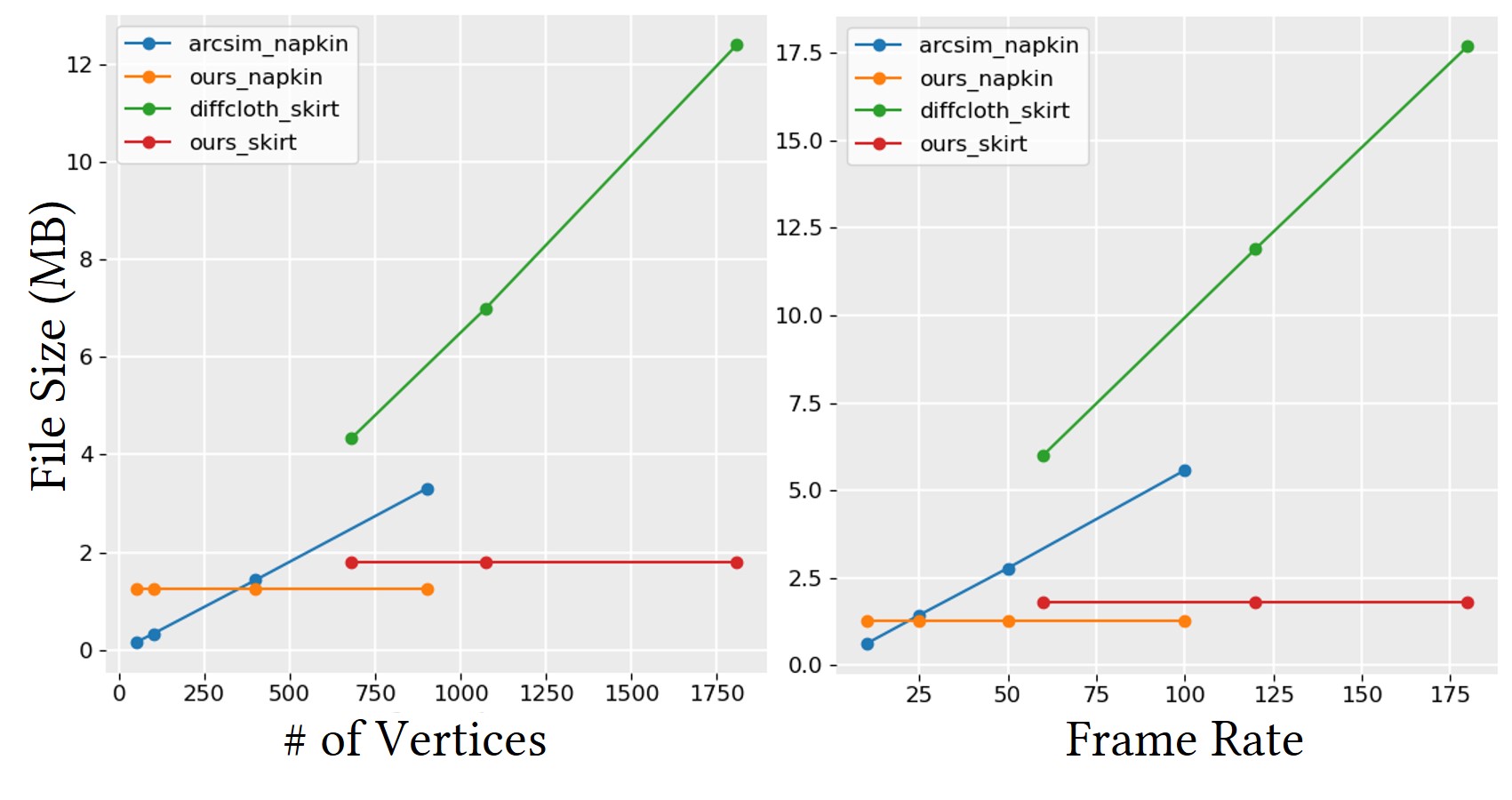
In the second numerical experiment, we evaluate the memory efficiency of several methods for simulations generated by NeuralClothSim, DiffARCSim (Liang et al., 2019) and DiffCloth (Li et al., 2022). The simulations are chosen to be of similar complexity and same length, and qualitative results are visualised in Fig. IX-appendix. In Fig. 8, we then plot the memory requirements as functions of spatial and temporal resolutions. Memory requirements are recorded for the 4D displacement fields, i.e., meshes over all time steps for the compared methods. In our case, the deformations are compactly stored as weights of the NDF network and we report the size of the latter. While the memory requirement of finite-element-based methods grows linearly as the function of 1) the number of vertices in the simulated cloth and 2) the total number of frames, our approach requires a constant and comparably small memory volume to store the dynamic simulations. Although memory efficiency is currently examined for shorter simulations, it presents great opportunities for extensions. We discuss simulations of longer duration in Appendix G. For better memory efficiency, existing simulators offer adaptive refinement (e.g., such as ARCSim) by re-meshing at each time step (coarse triangulation is used at smooth regions and fine meshes are used for wrinkles). However, they are not differentiable if re-meshing is performed. In contrast, our approach is adaptive without the overhead of re-meshing and without losing correspondence and differentiability due to re-meshing.

Physics-Informed Neural Networks for Shell Structures (Bastek and Kochmann, 2023).

Figure 9. Comparison of NeuralClothSim and (Bastek and Kochmann, 2023) on sleeve twisting (torsional movement of a cylindrical shell). While the cylinder in the simulation (a) twists without forming any wrinkles, our result (b) is correctly wrinkled similar to (Guo et al., 2018). The main reasons for the failure are linear strain and GELU activation functions that can capture smooth signals only.

In comparison to the quasi-static approach of (Bastek and Kochmann, 2023), our method performs dynamic simulation over time. Moreover, they consider thick shells and, therefore, learn a five-parameter Naghdi shell model (Naghdi, 1973) consisting of a 3D displacement and 2D rotation around the midsurface normal. Since cloths are thinner, we omit rotation similar to prior cloth simulators using Kirchhoff-Love theory (Clyde et al., 2017; Guo et al., 2018). Bastek et al. (2023) focus on engineering scenarios, and, to compare against them, we present their solutions for the Scordelis-Lo roof and a square plate in Tab. 3. We observe that the results of both our and their methods closely match the reference solutions. (Bastek and Kochmann, 2023) note instabilities during training a neural network conditioned on a point load, as it results in a sampling singularity at the point of application. Hence, in their pinched hemisphere example, they define the Gaussian force kernel centred at the midpoint instead of an exact point load. In contrast to theirs, we propose a new loss function for point loads (see Sec. 5.1) addressing the pinched cylinder obstacle course.

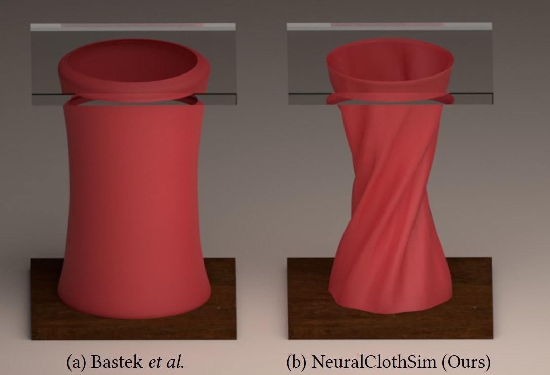
While (Bastek and Kochmann, 2023) show converged results on engineering examples, their method cannot capture the high-frequency signal (folds and wrinkles) required for cloth simulation. We next compare against them in the scenario of quasi-static twisting; the results are shown in Fig. 9. While their cylinder twists without forming any wrinkles, our result is correctly wrinkled similar to (Guo et al., 2018). The main reasons for the failure are 1) the linear strain and 2) that their activation function (GELU) can capture only smooth signals. Furthermore, while they use fixed samples, we re-sample in each iteration and continuously explore the full parametric domain, which also allows us to work with fewer samples.

5.4. Ablation

Figure 10. Contravariant vs Cartesian basis. Prediction of NDF output in the Cartesian coordinate system is well conditioned compared to the local covariant coordinate system. See Fig. 5 for further explanation of these coordinate systems.

Figure 11. Linear vs non-linear strain. We demonstrate napkin drooping under a downward force. Kirchhoff-Love strain is inherently highly non-linear. Linear approximation of it is often used in the small-strain regime, for quasi-static boundary value problems. However, without modelling non-linear strain, it is not possible to obtain satisfactory simulation dynamics (left), which contrasts with our solution modelling non-linear strain (right).

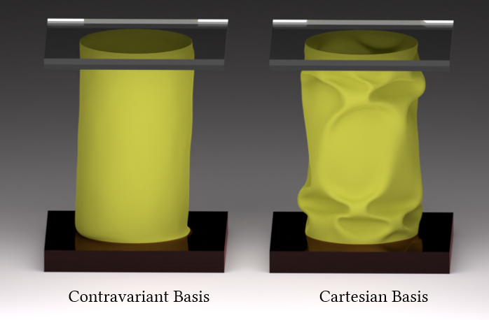
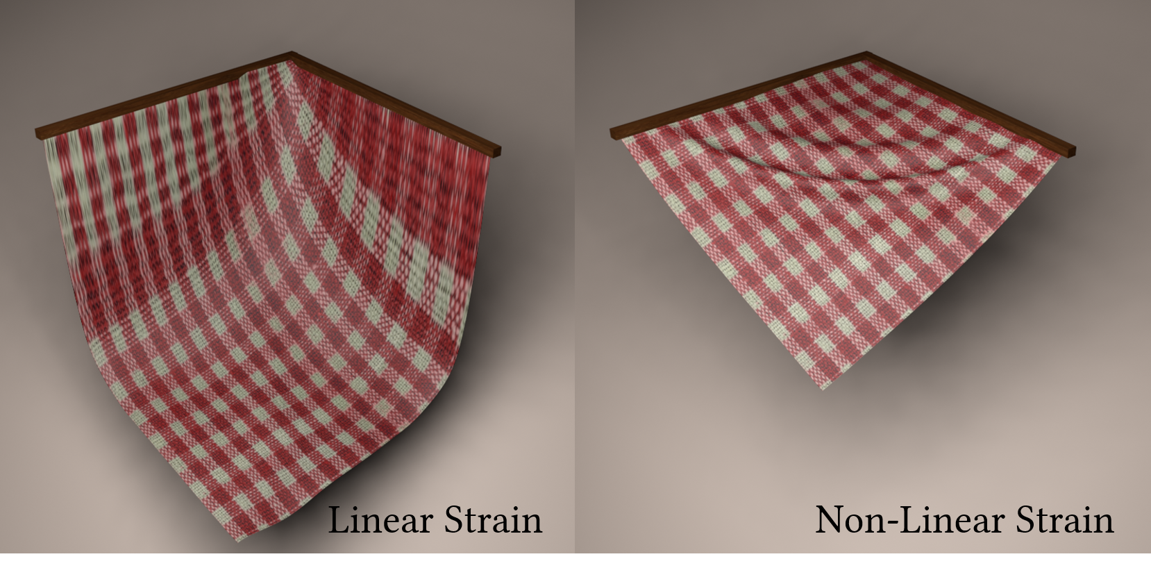
We conduct an ablative study on the choices made in the design and optimisation of the NDF to generate realistic cloth simulations. We evaluate the following variations (ablated versions) of our approach: 1) Concerning the choice of the coordinate system for NDF components as detailed in Sec. 4.1, and 2) Using a linear approximation of the strain energy density function (Sec. 4.3) instead of our model. We provide additional ablation results on boundary conditions and choice of activation functions for NDF in Tab. 3 and Appendix F.

NDF Coordinate System. Thin shell theory involves computing stretching and bending strains from deformations of the midsurface. In the Kirchhoff-Love formulation, strain energy computation is performed in the local contravariant (or covariant) basis. This leaves us with an obvious choice of predicting covariant components of NDF in locally varying (on the midsurface) contravariant basis (Fig. 5 shows such basis). Hence, (a) we predict NDF in a contravariant basis and use it directly in strain calculation and (b) we predict NDF in a global basis and transform its components to a local basis before strain calculation. The second case leverages the knowledge of local basis (rather than making the network guess it). We empirically observe that the prediction in a global Cartesian coordinate system leads to better convergence, as shown in Fig. 10.

Non-linearity of Strain Energy Density. In the quasi-static setting and in the small-strain regime, linearised kinematics is often employed (e.g., in engineering or structural mechanics). However, accurate simulation of cloth dynamics requires modelling of both rigid and non-rigid motion. Kirchhoff-Love membrane and bending strains are non-linear functions of the displacement field and non-linear strain calculation is decisive for obtaining the most accurate and realistic results. Thus, we evaluate the linear approximation of Kirchhoff-Love strain by omitting the non-linear terms in (30). In Fig. 11, we show that a linear approach leads to significant inaccuracies in modelling a piece of cloth bending under gravity.

5.5. Applications

Finally, we show a few applications of NeuralClothSim, i.e., learning material prior and simulation editing.

Non-linearity of Strain Energy Density. Our approach supports material conditioning and interpolation. As opposed to training with a single known material, NDF can be conditioned on the material space as they are typically low-dimensional. As described in Sec. 4.4, we train an NDF conditioned on cloth thickness and $\boldsymbol{\Phi}\in\{\rho,E,\nu\}\times[h_{\mathrm{min}},h_{\mathrm{max}}]$ with $h_{\mathrm{min}}=\qty{0.0005}{}$ and $h_{\mathrm{max}}=\qty{0.0025}{}$. We visualise the simulated result for $h=\{0.0005,0.0015,0.0025\}$, in Fig. 1-(bottom right). Additional results for other material parameters can be found in our supplemental video (at 4:30 min:sec).

Simulation editing with NDF.

Figure 12. Simulation editing with NeuralClothSim. Users can interrupt the NDF training anytime to redesign the scene parameters. Here, we show an example of a simulation pre-trained with a fixed reference state and external force. Once converged, we fine-tune the NDF with smoothly varying external force (top) or the pose of the reference geometry (bottom) in each iteration. Fine-tuning a pre-trained NDF with updated design parameters is faster and offers querying of physically-plausible intermediate simulations.

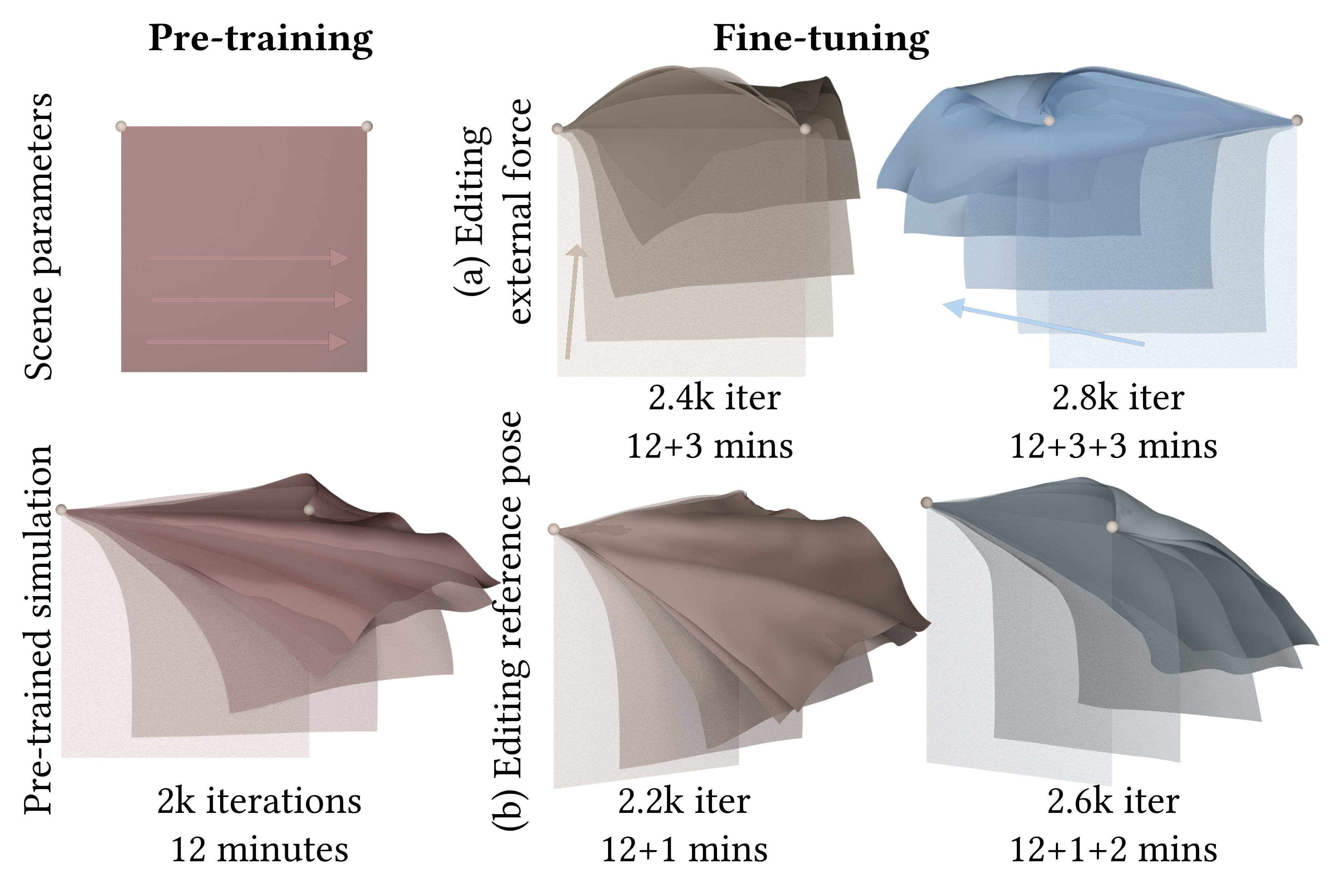
We next demonstrate results for dynamic editing of the pre-trained simulations. We conduct two experiments, i.e., editing external forces and editing the 6DoF pose of the reference geometry; the results are visualised in Fig. 12. First, a short simulation of a napkin is pre-trained as an NDF with a fixed reference state and external force, which takes ${\approx}12$ minutes. In the first example (top row), we gradually vary the direction and magnitude of the external force by linearly interpolating between the original and the final forces. This leads to the motion of cloth towards the instantaneous force direction.

In the second example (bottom row), we smoothly vary the reference poses and the corresponding position of the handles, generating novel edited simulations. Editing reference pose leads to the motion of the cloth towards a fixed force direction but originates from varying initial poses. Note how the change in the input scene parameters propagates to the entire simulation. Notably, fine-tuning is much faster and takes ${\approx}2$ minutes leading to a time-saving of ${\approx}83\%$. We show two intermediate simulations in Fig. 12 and other edited simulations corresponding to each iteration can be queried as well. Please refer to the supplementary video (at 4:40 min:sec) for visualisations of the additional intermediate results. As the simulation is parameterised by the weights of a neural network (instead of meshes), our proposed way of simulation editing is memory-efficient.

6. Discussion

This article addresses the fundamental challenges of differentiable cloth simulation with NDFs. All in all, we find the proposed design and the obtained experimental results very encouraging and see multiple avenues for future research. Currently, our simulator does not handle contacts, friction and collisions which will be necessary for many potential applications beyond those demonstrated in this article (e.g., cloth-object interaction). This is, however, a standalone research question in the new context (cf. Appendix J). Further, it should be possible to extend our framework with advanced models (non-linear and anisotropic) for the stress-strain relationship, to boost the realism and accuracy even further. Currently, our method efficiently supports short simulation scenarios (see Appendix G for an analysis of its performance).

Several limitations of NeuralClothSim originate from NDF modelling as a single MLP: First, we model the global space-time evolution in the network while classical simulators integrate forward in time, solving only for the next immediate state. This requires solving an optimisation problem with many degrees of freedom. Second, MLP weights have a global effect on the simulation, whereas the movement of mesh vertices affects only the local neighbourhood. While this global nature offers continuity and differentiability, we believe exploring alternative network parameterisations that bring the best of both representations could bring improvements in future. Finally, our results are currently of an empirical nature: While we observe expected results in all our experiments, there are no convergence guarantees or upper bounds on the accuracy.

Summa summarum, NeuralClothSim is the first step towards neural implicit cloth simulation, which we believe can become a powerful addition to the class of cloth simulators. Inverse problems in vision and graphics could also benefit from its consistency, differentiability and adaptivity. We urge the readers to watch our supplementary video for dynamic visualisations.

7. Conclusion

We present NeuralClothSim, a new cloth simulator operating on compact NDFs governed by the rules of the non-linear Kirchhoff-Love shell theory. Our method closely matches analytical values in several challenging experiments (such as an obstacle course) and enables, for the first time in cloth simulation, querying dynamic states of a thin shell continuously and consistently in space and time. The demonstrated results are physically-plausible across different scenarios under time-varying external forces and boundary motions; our method generates folds and wrinkles in the twisting of sleeves and diamond patterns in buckling experiments. Moreover, we propose an extended NDF allowing test-time interpolation of material properties and NDF editing (i.e., simulation editing).

In conclusion, we see NeuralClothSim as an exciting and important step towards continuous, differentiable, and physically-realistic cloth simulators of a new generation. While our simulator shows promising results and unprecedented characteristics compared to existing simulators, there is a long way to go until all traditional functionalities such as collision handling are unlocked. Yet, we believe it can pave the path towards an entirely new generation of physics simulation engines with their unique advantages.

NeuralClothSim: Neural Deformation Fields Meet the Kirchhoff-Love Thin Shell Theory (Appendix)

Table of Contents [sections] [sections]l1

Sections referenced with numbers refer to the main matter. All referenced figures and equations are per default from this document, unless they are followed by the “(main matter)” mark.

Appendix A Implementation Details

We implement NeuralClothSim in PyTorch (Paszke et al., 2019) and compute the geometric quantities on the reference shape and on the NDF using its tensor operations; the first and second-order derivatives are calculated using automatic differentiation. Our network architecture for NDF is an MLP with sine activations (SIREN) (Sitzmann et al., 2020) with five hidden layers and $512$ units in each layer. We empirically set SIREN’s frequency parameter to $\omega_{0}=15$ for all experiments (we observed that choosing $\omega_{0}=1$ does not permit folds). Although we sample from $(\xi^{1},\xi^{2})\in\Omega,t\in[0,T]$, we normalise samples $(\xi^{1},\xi^{2},t)\in[0,1]^{3}$ when feeding the input to MLP as per the initialisation principle of SIREN. Note that all physical quantities are computed in the original domains (e.g., $\Omega,[0,T]$) and the gradients are tracked in their scaled versions. For training, we use $N_{\Omega}=20{\times}20$ and $N_{t}=20$. At test time, we sample much higher for visualisation, usually with $N_{\Omega}=100{\times}100$ and $N_{t}=30$. For material conditioning, we use a single random material sample per training iteration. NeuralClothSim’s training time amounts to ${\sim}10$ minutes for most experiments, and the number of training iterations equals $2000$. We use ADAM (Kingma and Ba, 2014) optimiser with a learning rate of $10^{-4}$ and run our simulator on a single NVIDIA Quadro RTX 8000 GPU with 48 GB of global memory.

Appendix B Tensor Algebra

We provide additional results from tensor algebra (Wempner and Talaslidis, 2003)) that are relevant for strain computations on shells (see Sec. C).

Based on the coordinate system for the tensor components, a tensor can be covariant, (e.g., $A_{\alpha\beta}$), contravariant(e.g., $A^{\alpha\beta}$) and may even have mixed character (partly contravariant and partly covariant in different indices, e.g., $A_{\alpha}^{\beta}$). For computing $\varphi_{\beta}^{\lambda}$, and $\varphi^{\lambda}_{3}$ in (30)-(main matter), we use the following rule from shell theory that transforms a covariant tensor to a mixed one:

(40) $$\begin{split}A^{\alpha}_{\beta}&=A_{\beta\lambda}\bar{a}^{\lambda\alpha},\\ A^{\alpha}_{3}&=A_{\lambda 3}\bar{a}^{\lambda\alpha}.\end{split}$$

A tensor of n-th order has n indices. For example, $v_{\alpha}$ is first-order, and $H^{\beta\alpha\lambda\delta}$ is fourth. For computing the covariant derivatives of the first-order tensor $u_{\rho}|_{\alpha}$ and the second-order tensor $\varphi_{\alpha\lambda}|_{\beta}$ in (30), we use the following rules:

(41) $$\begin{split}&v_{\alpha}|_{\beta}=v_{\alpha,\beta}-v_{\lambda}\Gamma_{\alpha\beta}^{\lambda},\text{ and }\\ &A_{\alpha\beta}|_{\gamma}=A_{\alpha\beta,\gamma}-A_{\lambda\beta}\Gamma_{\alpha\gamma}^{\lambda}-A_{\alpha\lambda}\Gamma_{\beta\gamma}^{\lambda},\end{split}$$

where $\Gamma_{\alpha\beta}^{\lambda}$ is the Christoffel symbol given by

(42) $$\Gamma_{\alpha\beta}^{\lambda}:=\mathbf{\bar{a}}^{\lambda}\cdot\mathbf{\bar{a}}_{\alpha,\beta}.$$

Some tensors arising in the kinematic description of Kirchhoff-Love thin shells are symmetric with respect to indices $\alpha$ and $\beta$, i.e., $A_{\alpha\beta}=A_{\beta\alpha}$. We exploit the symmetry for efficient computations of the following tensors: $a_{\alpha\beta}$, $b_{\alpha\beta}$, $\varepsilon_{\alpha\beta}$, $\kappa_{\alpha\beta}$, and $\Gamma_{\alpha\beta}^{\lambda}$.

We also exploit the symmetry of fourth-order symmetric tensor $\mathbf{H}$:

$$H^{\alpha\beta\lambda\delta}=H^{\beta\alpha\lambda\delta}=H^{\beta\alpha\delta\lambda}=H^{\alpha\beta\delta\lambda}=H^{\lambda\delta\alpha\beta}.$$

This property means that only six independent components (after applying symmetry) need to be computed (i.e., $H^{1111}$, $H^{1112}$, $H^{1122}$, $H^{1212}$, $H^{1222}$, and $H^{2222}$).

Appendix C Proof of Strain Computation

According to the Kirchhoff-Love theory, the Green-Lagrange strain associated with the deformation of a thin shell is decomposed into the stretching and bending strains of the midsurface. One could compute them using Eqs. (15) and (16)-(main matter), written in terms of the reference state $\bar{\mathbf{x}}$ and the deformed state $\mathbf{x}$ of the midsurface. As an easier alternative, we directly evaluate strains with the NDF $\mathbf{u}$ of the midsuface using (30)-(main matter). Next, we prove that the two formulations are identical following (Basar and Krätzig, 2013)).

Lemma C.1 (Deformation gradient).

Deformation gradient $\mathbf{u}_{,\alpha}$ can be written as $\mathbf{u}_{,\alpha}=\varphi_{\alpha\lambda}\mathbf{\bar{a}}^{\lambda}+\varphi_{\alpha 3}\mathbf{\bar{a}}^{3}$ where the components of the gradients $\varphi_{\alpha\lambda},\varphi_{\alpha 3}$ are defined as

(43) $$\begin{split}\varphi_{\alpha\lambda}&:=u_{\lambda}|_{\alpha}-\bar{b}_{\alpha\lambda}u_{3},\text{ and }\\ \varphi_{\alpha 3}&:=u_{3,\alpha}+\bar{b}_{\alpha}^{\lambda}u_{\lambda}.\end{split}$$

Proof.

Given deformation field $\mathbf{u}$ of the midsurface described in contravariant basis as $\mathbf{u}=u_{\lambda}\mathbf{\bar{a}}^{\lambda}+u_{3}\mathbf{\bar{a}}^{3}$ , we compute the deformation gradient as follows:

(44) $$\begin{split}\mathbf{u}_{,\alpha}=\mathbf{u}|_{\alpha}&=u_{\lambda}|_{\alpha}\mathbf{\bar{a}}^{\lambda}+u_{\lambda}\mathbf{\bar{a}}^{\lambda}|_{\alpha}+u_{3}|_{\alpha}\mathbf{\bar{a}}^{3}+u_{3}\mathbf{\bar{a}}^{3}|_{\alpha}\\ &=u_{\lambda}|_{\alpha}\mathbf{\bar{a}}^{\lambda}+u_{\lambda}\bar{b}_{\alpha}^{\lambda}\mathbf{\bar{a}}^{3}+u_{3,\alpha}\mathbf{\bar{a}}^{3}-u_{3}\bar{b}_{\alpha\lambda}\mathbf{\bar{a}}^{\lambda},\end{split}$$

where we use the following identities from the shell theory (Basar and Krätzig, 2013) to arrive at the bottom part of the previous equation:

(45) $$\begin{split}&\mathbf{\bar{a}}^{3}|_{\alpha}=\mathbf{\bar{a}}^{3}_{,\alpha}=-\bar{b}_{\alpha\lambda}\mathbf{\bar{a}}^{\lambda}=-\bar{b}_{\alpha}^{\lambda}\bar{\mathbf{a}}_{\lambda},\\ &\mathbf{\bar{a}}^{\lambda}|_{\alpha}=\bar{b}_{\alpha}^{\lambda}\mathbf{\bar{a}}^{3}.\end{split}$$

Finally, we rewrite them as

(46) $$\mathbf{u}_{,\alpha} =\varphi_{\alpha\lambda}\mathbf{\bar{a}}^{\lambda}+\varphi_{\alpha 3}\mathbf{\bar{a}}^{3}.$$

∎

Theorem C.2 (Membrane strain).

Membrane strain (quantifying/measuring in-plane stretching) can be written as a function of the deformation gradient in the following form:

(47) $$\varepsilon_{\alpha\beta} =\frac{1}{2}(\varphi_{\alpha\beta}+\varphi_{\beta\alpha}+\varphi_{\alpha\lambda}\varphi_{\beta}^{\lambda}+\varphi_{\alpha 3}\varphi_{\beta 3}).$$

Proof.

We start with membrane strain given as the difference of metric tensors (first fundamental form) (15):

(48) $$\begin{split}\varepsilon_{\alpha\beta}&:=\frac{1}{2}(a_{\alpha\beta}-\bar{a}_{\alpha\beta}),\\ \varepsilon_{\alpha\beta}&=\frac{1}{2}(\mathbf{a}_{\alpha}\cdot\mathbf{a}_{\beta}-\bar{\mathbf{a}}_{\alpha}\cdot\bar{\mathbf{a}}_{\beta}).\end{split}$$

Substituting the tangent basis vectors $\mathbf{a}_{\alpha}$

(49) $$\begin{split}\mathbf{a}_{\alpha}=\mathbf{x},_{\alpha}=\bar{\mathbf{x}},_{\alpha}+\mathbf{u},_{\alpha}=\bar{\mathbf{a}}_{\alpha}+\mathbf{u},_{\alpha}\end{split}$$

gives us updated strain in terms of deformation $\mathbf{u}$:

(50) $$\varepsilon_{\alpha\beta}=\frac{1}{2}(\bar{\mathbf{a}}_{\alpha}\cdot\mathbf{u,_{\beta}}+\bar{\mathbf{a}}_{\beta}\cdot\mathbf{u,_{\alpha}}+\mathbf{u},_{\alpha}\cdot\mathbf{u},_{\beta}).$$

Assuming the following identities from Kirchhoff-Love shell hypothesis (Basar and Krätzig, 2013):

(51) $$\begin{split}&\bar{\mathbf{a}}_{\alpha}\cdot\bar{\mathbf{a}}^{\beta}=\delta^{\beta}_{\alpha},\bar{\mathbf{a}}^{3}=\bar{\mathbf{a}}_{3},\bar{\mathbf{a}}_{\alpha}\cdot\bar{\mathbf{a}}^{3}=\bar{\mathbf{a}}^{\alpha}\cdot\bar{\mathbf{a}}_{3}=0,\bar{\mathbf{a}}^{3}\cdot\bar{\mathbf{a}}^{3}=1,\text{ and }\\ &\bar{a}^{\alpha\beta}=\bar{\mathbf{a}}^{\alpha}\cdot\bar{\mathbf{a}}^{\beta},A^{\alpha}_{\beta}=A_{\beta\lambda}\bar{a}^{\lambda\alpha},\end{split}$$

and considering the above lemma for the deformation gradient $\mathbf{u}_{,\alpha}$, we finally obtain the target formulation for strain:

(52) $$\varepsilon_{\alpha\beta} =\frac{1}{2}(\varphi_{\alpha\beta}+\varphi_{\beta\alpha}+\varphi_{\alpha\lambda}\varphi_{\beta}^{\lambda}+\varphi_{\alpha 3}\varphi_{\beta 3}).$$

∎

Theorem C.3 (Bending strain).

Bending strain (measuring the change in curvature) can be written as a function of the deformation gradient in the following form:

(53) $$\kappa_{\alpha\beta}\approx-\varphi_{\alpha 3}|_{\beta}-\bar{b}_{\beta}^{\lambda}\varphi_{\alpha\lambda}+\varphi^{\lambda}_{3}(\varphi_{\alpha\lambda}|_{\beta}+\frac{1}{2}\bar{b}_{\alpha\beta}\varphi_{\lambda 3}-\bar{b}_{\beta\lambda}\varphi_{\alpha 3}).$$

Proof.

Analogous to the deformation field $\mathbf{u}:=\mathbf{x}-\bar{\mathbf{x}}$ of the midsurface, we define $\mathbf{w}$ as the difference vector of unit normals to the midsurface, i.e.,

(54) $$\mathbf{w}:=\mathbf{a}_{3}-\bar{\mathbf{a}}_{3}=w_{\lambda}\mathbf{\bar{a}}^{\lambda}+w_{3}\mathbf{\bar{a}}^{3}=w^{\lambda}\mathbf{\bar{a}}_{\lambda}+w^{3}\mathbf{\bar{a}}_{3}.$$

Using this formulation, points on the deformed shell continuum can be described by the field $\mathbf{\tilde{u}}(\xi^{1},\xi^{2},\xi^{3})=\mathbf{u}(\xi^{1},\xi^{2})+\xi^{3}\mathbf{w}(\xi^{1},\xi^{2})$. The difference vector $\mathbf{w}$ describes the change in the orientation of midsurface, enabling us to quantify bending.

The bending strain of the midsurface is defined as the difference of curvature tensors (second fundamental form) in the reference and deformed configurations:

(55) $$\begin{split}\kappa_{\alpha\beta}&:=\bar{b}_{\alpha\beta}-b_{\alpha\beta}\\ \kappa_{\alpha\beta}&=\mathbf{a}_{\alpha}\cdot\mathbf{a}_{3,\beta}-\bar{\mathbf{a}}_{\alpha}\cdot\bar{\mathbf{a}}_{3,\beta}\end{split}$$

Using (49) and (54), we rewrite strain using deformation gradients as:

(56) $$\kappa_{\alpha\beta} =(\bar{\mathbf{a}}_{\alpha}+\mathbf{u,_{\alpha}})\cdot(\bar{\mathbf{a}}_{3,\beta}+\mathbf{w,_{\beta}})-\bar{\mathbf{a}}_{\alpha}\cdot\bar{\mathbf{a}}_{3,\beta}$$

Further simplification and applying identity (45) leads to:

(57) $$\kappa_{\alpha\beta} =\bar{\mathbf{a}}_{\alpha}\cdot\mathbf{w,_{\beta}}+\mathbf{u,_{\alpha}}\cdot\mathbf{w,_{\beta}}-\bar{b}_{\beta}^{\lambda}\mathbf{u,_{\alpha}}\cdot\bar{\mathbf{a}}_{\lambda}$$

Using Lemma C.1 for deformation gradients $\mathbf{u}_{,\alpha}$ and $\mathbf{w}_{,\beta}$, i.e, $\mathbf{w}_{,\beta}=(w_{\lambda}|_{\beta}-\bar{b}_{\lambda\beta}w_{3})\mathbf{\bar{a}}^{\lambda}+(w_{3,\beta}+\bar{b}_{\beta}^{\lambda}w_{\lambda})\mathbf{\bar{a}}^{3}$ and with the shell identities of (51), we arrive at:

(58) $$\begin{split}\kappa_{\alpha\beta}=w_{\alpha}|_{\beta}-\bar{b}_{\alpha\beta}w_{3}-\bar{b}_{\beta}^{\lambda}\varphi_{\alpha\lambda}+\varphi_{\alpha}^{\lambda}(w_{\lambda}|_{\beta}-\bar{b}_{\lambda\beta}w_{3})\\ +\varphi_{\alpha 3}(w_{3,\beta}+\bar{b}_{\beta}^{\lambda}w_{\lambda})\end{split}$$

With the Kirchhoff-Love normal hypothesis and neglecting cubic terms, we can approximate the components of $\mathbf{w}$ as the following:

(59) $$\begin{split}w_{3}\approx-\frac{1}{2}w_{\lambda}w^{\lambda},\\ w_{\alpha}\approx-\varphi_{\alpha 3}+\varphi_{\alpha}^{\lambda}\varphi_{\lambda 3}.\end{split}$$

First eliminating the component $w_{3}$ and subsequently $w_{\alpha}$, we arrive at the target strain formulation:

(60) $$\begin{split}\kappa_{\alpha\beta}\approx w_{\alpha}|_{\beta}-\bar{b}_{\beta}^{\lambda}\varphi_{\alpha\lambda}+\frac{1}{2}\bar{b}_{\alpha\beta}w_{\lambda}w^{\lambda}+w^{\lambda}|_{\beta}\varphi_{\alpha\lambda}+\bar{b}_{\beta}^{\lambda}w_{\lambda}\varphi_{\alpha 3}\\ \kappa_{\alpha\beta}\approx-\varphi_{\alpha 3}|_{\beta}-\bar{b}_{\beta}^{\lambda}\varphi_{\alpha\lambda}+\varphi^{\lambda}_{3}(\varphi_{\alpha\lambda}|_{\beta}+\frac{1}{2}\bar{b}_{\alpha\beta}\varphi_{\lambda 3}-\bar{b}_{\beta\lambda}\varphi_{\alpha 3}).\end{split}$$

∎

Figure I. Belytschko obstacle course: Visualisation of the deformation fields predicted by our NeuralClothSim. From the left to the right: Square plate, Scordelis-Lo roof, pinched cylinder with fixed boundary conditions and pinched cylinder with free boundary conditions. For the pinched cylinder, the results are re-scaled versions with $E=\qty{30}{}$.

Appendix D Belytschko Obstacle Course

In the following, we provide detailed information for reproducing the Belytschko obstacle course experiments from Sec. 5.1-(main matter). We visualise the NDF along the direction of applied load in Fig. I that closely matches the reference solutions (Belytschko et al., 1985).

D.1. Square Plate

The reference geometry of the square plate is given by (23)-(main matter) with $L=\qty{100}{},h=\qty{1}{}$. Concerning the boundary conditions, the plate is simply supported along the boundary curve (defined by $\partial\Omega=\{(\xi^{1},0),(0,\xi^{2}),(\xi^{1},L),(L,\xi^{2})\}$). Next, we set material properties as $E=\qty{1e7}{}$ and $\nu=0$ and apply a uniformly distributed load (force) $\mathbf{f}=[0,0,-1]^{\top}$. We optimise NDF under boundary conditions as follows:

(61) $$\begin{split}&\mathbf{u}(\boldsymbol{\xi};\Theta)=\mathcal{F}_{\Theta}(\boldsymbol{\xi})\mathcal{B}(\boldsymbol{\xi}),\\ \text{ s.t. }&\mathcal{B}(\boldsymbol{\xi}):=\xi^{1}\xi^{2}(L-\xi^{1})(L-\xi^{2}).\end{split}$$

Our loss function for training is of the following form:

(62) $$\begin{split}\mathcal{L}&=\frac{|\Omega|}{N_{\Omega}}\sum_{i=1}^{N_{\Omega}}\Big{(}\frac{1}{2}D\boldsymbol{\varepsilon}^{\top}(\boldsymbol{\xi}_{i})\mathbf{H}(\boldsymbol{\xi}_{i})\boldsymbol{\varepsilon}(\boldsymbol{\xi}_{i})+\\ &+\frac{1}{2}B\boldsymbol{\kappa}^{\top}(\boldsymbol{\xi}_{i})\mathbf{H}(\boldsymbol{\xi}_{i})\boldsymbol{\kappa}(\boldsymbol{\xi}_{i})-\mathbf{f}^{\top}(\boldsymbol{\xi}_{i})\mathbf{u}(\boldsymbol{\xi}_{i})\Big{)}\sqrt{\bar{a}(\boldsymbol{\xi}_{i})}.\end{split}$$

Fig. I-(left) shows the obtained NDF along the $z$-axis for the square plate.

D.2. Scordelis-Lo Roof

The reference geometry of the Scordelis-Lo roof is given by the following parametric expression:

(63) $$\begin{split}&\mathbf{\bar{x}}(\boldsymbol{\xi})=[R\cos(\xi^{1}+\qty{50}{}),R\sin(\xi^{1}+\qty{50}{}),\xi^{2}]^{\top},\\ &\forall\xi^{1}\in[0,\qty{80}{});\xi^{2}\in[0,L],\text{ with }\\ &R=\qty{25}{},L=\qty{50}{},\text{ and }h=\qty{0.25}{}.\end{split}$$

Concerning the boundary conditions, the structure is supported with a rigid diaphragm along the edges, i.e., $\partial\Omega=\{(\xi^{1},0),(\xi^{1},L)\}$. The material properties are set as $E=\qty{4.32e8}{},\nu=0$ and a uniformly distributed load $\mathbf{f}=[0,-90,0]^{\top}$ is applied to it.

We optimise NDF under boundary conditions as follows:

(64) $$\begin{split}&\mathbf{u}(\boldsymbol{\xi};\Theta)=[\mathcal{F}_{\Theta 1}\mathcal{B}(\boldsymbol{\xi}),\mathcal{F}_{\Theta 2}\mathcal{B}(\boldsymbol{\xi}),\mathcal{F}_{\Theta 3}]^{\top},\\ \text{ s.t. }&\mathcal{B}(\boldsymbol{\xi}):=\xi^{2}(L-\xi^{2}).\end{split}$$

The loss function is the same as in (D.1) for the square plate case. Fig. I-(second on the left) visualises the computed NDF along the $y$-axis.

D.3. Pinched Cylinder

We consider two cases: 1) a cylinder with ends constrained by rigid diaphragms and 2) a cylinder with free ends.

The reference geometry in both cases is given by (24)-(main matter) with $R=\qty{300}{},L=\qty{600}{},h=\qty{3}{}.$ The constrained cylinder is supported with a rigid diaphragm along the edges, i.e., $\partial\Omega=\{(\xi^{1},0),(\xi^{1},L)\}$; for the cylinder with free ends $\partial\Omega=\emptyset$. The material properties are set as $E=\qty{3e6}{},\nu=0.3$. We apply point loads $\mathbf{f}\in\{[0,0,1]^{\top},[0,0,-1]^{\top}\}$ at diametrically opposite points $\Omega_{0}=\{(\qty{90}{},300),(\qty{270}{},300)\}$. Next—due to periodicity of the geometry—we define NDF as $\mathcal{F}_{\Theta}(\cos\xi^{1},\sin\xi^{1},\xi^{2})$ (instead of the default case $\mathcal{F}_{\Theta}(\xi^{1},\xi^{2})$).

In the first case (rigid diaphragms), we optimise NDF using

(65) $$\begin{split}&\mathbf{u}(\boldsymbol{\xi};\Theta)=[\mathcal{F}_{\Theta 1}\mathcal{B}(\boldsymbol{\xi}),\mathcal{F}_{\Theta 2},\mathcal{F}_{\Theta 3}\mathcal{B}(\boldsymbol{\xi})]^{\top},\\ \text{ s.t. }&\mathcal{B}(\boldsymbol{\xi}):=\xi^{2}(L-\xi^{2}).\end{split}$$

In the second case (free ends), the NDF parametrisation factors out the rigid motion and therefore reads as:

(66) $$\begin{split}\mathbf{u}(\boldsymbol{\xi};\Theta)&=[\mathcal{F}_{\Theta 1}\mathcal{B}_{1}(\boldsymbol{\xi})\mathcal{B}_{2}(\boldsymbol{\xi}),\mathcal{F}_{\Theta 2}\mathcal{B}_{1}(\boldsymbol{\xi})\mathcal{B}_{2}(\boldsymbol{\xi}),\mathcal{F}_{\Theta 3}]^{\top},\\ \text{ s.t. }\mathcal{B}_{1}(\boldsymbol{\xi})&:=1-e^{-((\xi^{1}-\qty{90}{})^{2}+(\xi^{2}-300)^{2})/\sigma},\text{ and }\\ \mathcal{B}_{2}(\boldsymbol{\xi})&:=1-e^{-((\xi^{1}-\qty{270}{})^{2}+(\xi^{2}-300)^{2})/\sigma}.\end{split}$$

Finally, the loss function in both cases reads:

(67) $$\mathcal{L} =\frac{|\Omega|}{N_{\Omega}}\sum_{i=1}^{N_{\Omega}}\Big{(}\frac{1}{2}D\boldsymbol{\varepsilon}^{\top}(\boldsymbol{\xi}_{i})\mathbf{H}(\boldsymbol{\xi}_{i})\boldsymbol{\varepsilon}(\boldsymbol{\xi}_{i})$$

$$+\frac{1}{2}B\boldsymbol{\kappa}^{\top}(\boldsymbol{\xi}_{i})\mathbf{H}(\boldsymbol{\xi}_{i})\boldsymbol{\kappa}(\boldsymbol{\xi}_{i})\Big{)}\sqrt{\bar{a}(\boldsymbol{\xi}_{i})}-\sum_{\boldsymbol{\xi}\in\Omega_{0}}\mathbf{f}^{\top}(\boldsymbol{\xi})\mathbf{u}(\boldsymbol{\xi}).$$

Fig. I-(second from the right, and the rightmost) shows the obtained NDFs along the $z$-axis for the two cases of the pinched cylinder.

Figure II. Ablation study for boundary conditions, with Dirichlet (top) and periodic (bottom) boundary conditions.

Figure III. Results of our method with different activation functions (ReLU, GELU and Siren).

Figure IV. Runtime analysis of NeuralClothSim. On the left, we visualise the evolution of the last frame over the training iterations. On the right, the plot shows NDF convergence as a function of training time leading to refined simulations.

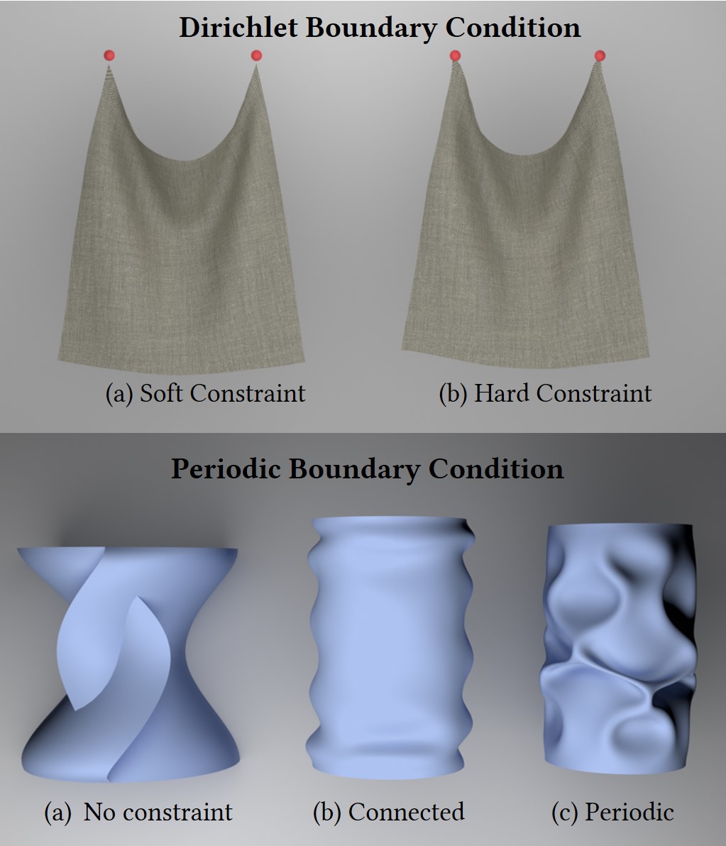
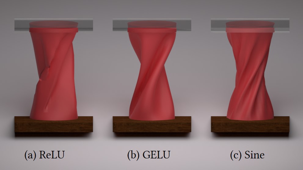
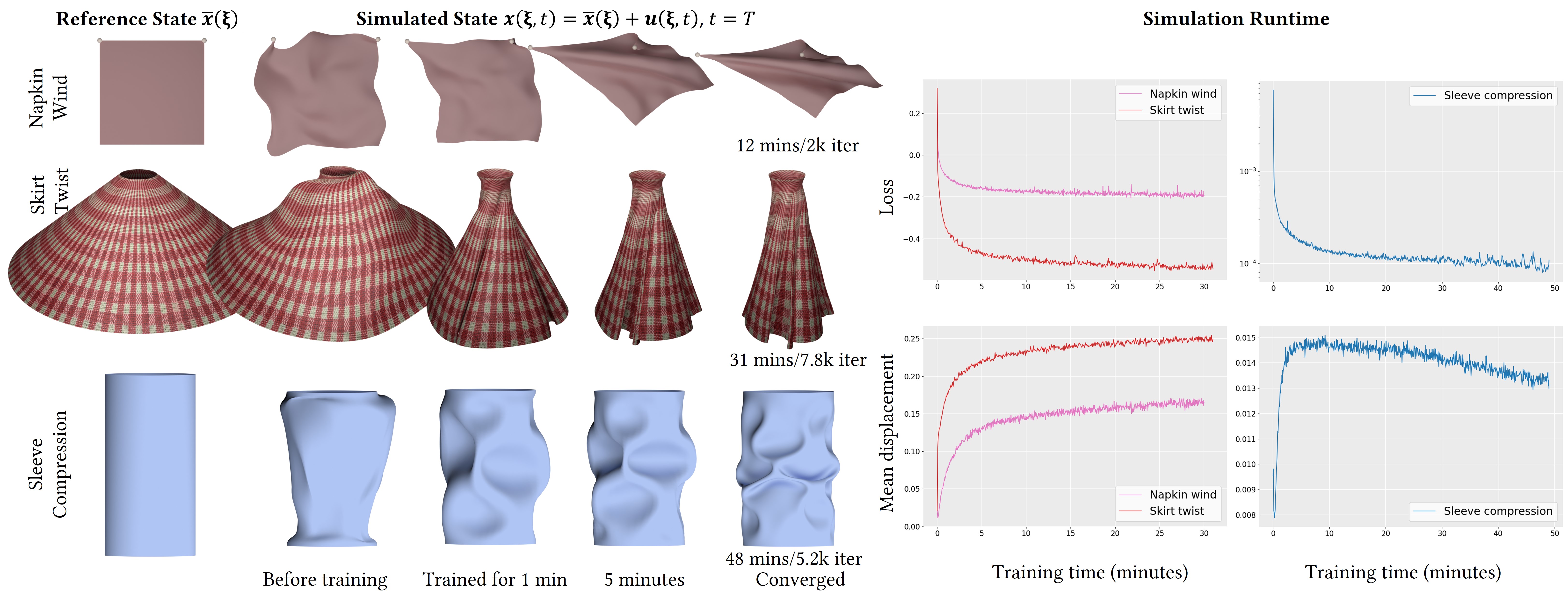
Appendix E Simulation Details

Similar to the previous section, we provide boundary and loading conditions for all experiments here. We refer to the figures in the main document.

E.1. Napkin

The force in this experiment is defined as $\mathbf{f}=[0,-9.8\rho,0]^{\top}$ and the boundary conditions read $\partial\Omega=\{(0,0),(0,L)\}$. The result of a napkin droop with a fixed corner is shown in Fig. 1-(main matter). NDF in this experiment is parametrised as follows:

(68) $$\begin{split}&\mathbf{u}(\boldsymbol{\xi},t;\Theta)=\mathcal{F}_{\Theta}(\boldsymbol{\xi},t)\mathcal{I}(t)\mathcal{B_{\mathrm{top\_left\_corner}}}(\boldsymbol{\xi}),\\ \text{ s.t. }&\mathcal{B_{\mathrm{top\_left\_corner}}}(\xi^{1},\xi^{2}):=1-e^{-((\xi^{1})^{2}+(\xi^{2}-L)^{2})/\sigma}.\end{split}$$

The experimental result of a napkin droop with moving corners is shown in Fig. 3-(main matter). The boundary condition read $\partial\Omega=\{(0,L),(L,L)\}$. The NDF parametrisation in this scenario is as follows:

(69) $$\begin{split}&\mathbf{u}=\mathcal{F}_{\Theta}\mathcal{I}\mathcal{B_{\mathrm{top\_left}}}\mathcal{B_{\mathrm{top\_right}}}+\\ &+(1-\mathcal{B_{\mathrm{top\_left}}})\mathcal{B_{\mathrm{motion}}}-(1-\mathcal{B_{\mathrm{top\_right}}})\mathcal{B_{\mathrm{motion}}},\\ &\text{ s.t. }\mathcal{B_{\mathrm{top\_left}}}(\xi^{1},\xi^{2}):=1-e^{-((\xi^{1})^{2}+(\xi^{2}-L)^{2})/\sigma},\\ &\mathcal{B_{\mathrm{top\_right}}}(\xi^{1},\xi^{2}):=1-e^{-((\xi^{1}-L)^{2})+(\xi^{2}-L)^{2})/\sigma},\text{ and }\\ &\mathcal{B_{\mathrm{motion}}}(t):=[0.2t,0,0]^{T}.\end{split}$$

The experimental result for napkin droop with fixed edges is shown in Fig. 11. The boundary conditions are defined as $\partial\Omega=\{(\xi^{1},0),(0,\xi^{2})\},\forall(\xi^{1},\xi^{2})\in[0,L]^{2}$ and the NDF parameterisation reads

(70) $$\begin{split}&\mathbf{u}=\mathcal{F}_{\Theta}\mathcal{I}\mathcal{B_{\mathrm{left\_edge}}}\mathcal{B_{\mathrm{right\_edge}}}\\ \text{ s.t. }&\mathcal{B_{\mathrm{left\_edge}}}(\xi^{1}):=1-e^{-(\xi^{1})^{2}/\sigma},\text{ and }\\ &\mathcal{B_{\mathrm{right\_edge}}}(\xi^{2}):=1-e^{-(\xi^{2})^{2}/\sigma}.\end{split}$$

E.2. Sleeve

In the experiment with a sleeve, no external force is exerted: $\mathbf{f}=[0,0,0]^{T}$. The boundary region is defined by: $\partial\Omega=\{(\xi^{1},0),(\xi^{1},L)\},\forall\xi^{1}\in[0,2\pi)$. We demonstrate sleeve compression in Fig. 10-(main matter) and 4-(main matter). The NDF is parametrised as follows:

(71) $$\begin{split}&\mathbf{u}=\mathcal{F}_{\Theta}\mathcal{I}\mathcal{B_{\mathrm{bottom\_rim}}}\mathcal{B_{\mathrm{top\_rim}}}\\ &+(1-\mathcal{B_{\mathrm{bottom\_rim}}})\mathcal{B_{\mathrm{motion}}}-(1-\mathcal{B_{\mathrm{top\_rim}}})\mathcal{B_{\mathrm{motion}}},\\ \text{ s.t. }&\mathcal{B_{\mathrm{bottom\_rim}}}(\xi^{2}):=1-e^{-(\xi^{2})^{2}/\sigma},\\ &\mathcal{B_{\mathrm{top\_rim}}}(\xi^{2}):=1-e^{-(\xi^{2}-L)^{2}/\sigma},\text{ and }\\ &\mathcal{B_{\mathrm{motion}}}(t):=[0,0.1t,0]^{\top}.\end{split}$$

Sleeve twist is achieved by introducing rotation displacement $\theta=\frac{3\pi}{4}$. The NDF in this scenario is parametrised as follows:

(72) $$\begin{split}&\mathbf{u}=\mathcal{F}_{\Theta}\mathcal{I}(1-\mathcal{B_{\mathrm{bottom\_rim}}})(1-\mathcal{B_{\mathrm{top\_rim}}})\\ &-\mathcal{B_{\mathrm{bottom\_rim}}}\mathcal{B_{\mathrm{bottom\_motion}}}+\mathcal{B_{\mathrm{top\_rim}}}\mathcal{B_{\mathrm{top\_motion}}},\\ \text{ s.t. }&\mathcal{B_{\mathrm{bottom\_rim}}}(\xi^{2}):=e^{-(\xi^{2})^{2}/\sigma},\\ &\mathcal{B_{\mathrm{top\_rim}}}(\xi^{2}):=e^{-(\xi^{2}-L)^{2}/\sigma},\\ &\mathcal{B_{\mathrm{bottom\_motion}}}(\xi^{1},t):=\begin{bmatrix}R(\cos(\xi^{1}-\theta t)-\cos\xi^{1})\\ 0\\ R(\sin(\xi^{1}-\theta t)-\sin\xi^{1})\end{bmatrix},\text{ and }\\ &\mathcal{B_{\mathrm{top\_motion}}}(\xi^{1},t):=\begin{bmatrix}R(\cos(\xi^{1}+\theta t)-\cos\xi^{1})\\ 0\\ R(\sin(\xi^{1}+\theta t)-\sin\xi^{1})\end{bmatrix}.\end{split}$$

E.3. Skirt

See Fig. IX for the experimental results with skirt. The reference skirt geometry is defined as:

(73) $$\begin{split}\mathbf{\bar{x}}(\boldsymbol{\xi})&=[r\cos\xi^{1},\xi^{2},r\sin\xi^{1}]^{T},\;\forall\xi^{1}\in[0,2\pi);\xi^{2}\in[0,L],\\ \text{ s.t. }r(\xi^{2})&:=\frac{(R_{\mathrm{top}}-R_{\mathrm{bottom}})\xi^{2}}{L}+R_{\mathrm{bottom}}.\end{split}$$

The skirt deform in this experiment under gravity, i.e., $\mathbf{f}=[0,-9.8\rho,0]^{T}$; the boundary region is given by $\partial\Omega=\{(\xi^{1},L)\},\forall\xi^{1}\in[0,2\pi)$. NDF is parametrised as follows:

(74) $$\begin{split}&\mathbf{u}=\mathcal{F}_{\Theta}\mathcal{I}(1-\mathcal{B_{\mathrm{top\_rim}}}),\\ \text{ s.t. }&\mathcal{B_{\mathrm{top\_rim}}}(\xi^{2}):=e^{-(\xi^{2}-L)^{2}/\sigma}.\end{split}$$

The conditions for skirt twisting (angular displacement) are similar to those of the sleeve twist (applied at the top rim) in Sec. E.2.

Figure V. NeuralClothSim’s scalability with simulation length. We show the behaviour of our approach for longer simulation times. While we observe that the simulations of up to eight seconds converge after a few hours, our architecture would require modifications for a longer duration.

Figure VI. Training behaviour of NeuralClothSim for varying thickness values.

Figure VII. Analysis of the sampling strategies. We show the influence of the number of training points on the performance of our method.

Figure VIII. Runtime comparison of DiffARCSim (Liang et al., 2019) and our approach. Like most classical simulators, DiffARCSim integrates forward in time, solving for a 3D deformation field at each time step, in contrast to our approach which optimises for the 4D spatio-temporal NDF. With decreasing computational budget, DiffARCSim produces converged simulated states of the cloth at low resolutions or only early frames at high resolutions. On the other hand, NeuralClothSim offers partially converged simulations at arbitrary resolutions as the computational budget decreases.

Figure IX. Spatial and temporal surface consistency of state-of-the-art differentiable simulators and our approach. Classical simulators such as ARCSim (Liang et al., 2019) and DiffCloth (Li et al., 2022) reproduce simulation outcomes when re-running at the same resolution. However, changing spatio-temporal resolution requires multiple runs and generates possibly different folds or wrinkles instead of refining (or previewing) the geometry. Since we learn a continuous neural parameterised model, a converged (or partially converged) NDF provides consistent simulation when queried at different spatio-temporal inputs. Note that NeuralClothSim does not provide consistent refinement as a function of computation time (no speed vs fidelity trade-off), but rather consistent simulation with respect to the spatio-temporal sampling (at a given computational budget).

Figure X. Limitations. Our approach does not handle collisions, contacts and frictions at the moment, since the focus of this work is on the fundamental challenges of developing a neural cloth simulator. These examples show inaccuracies due to the simplifications made in one possible extension (75).

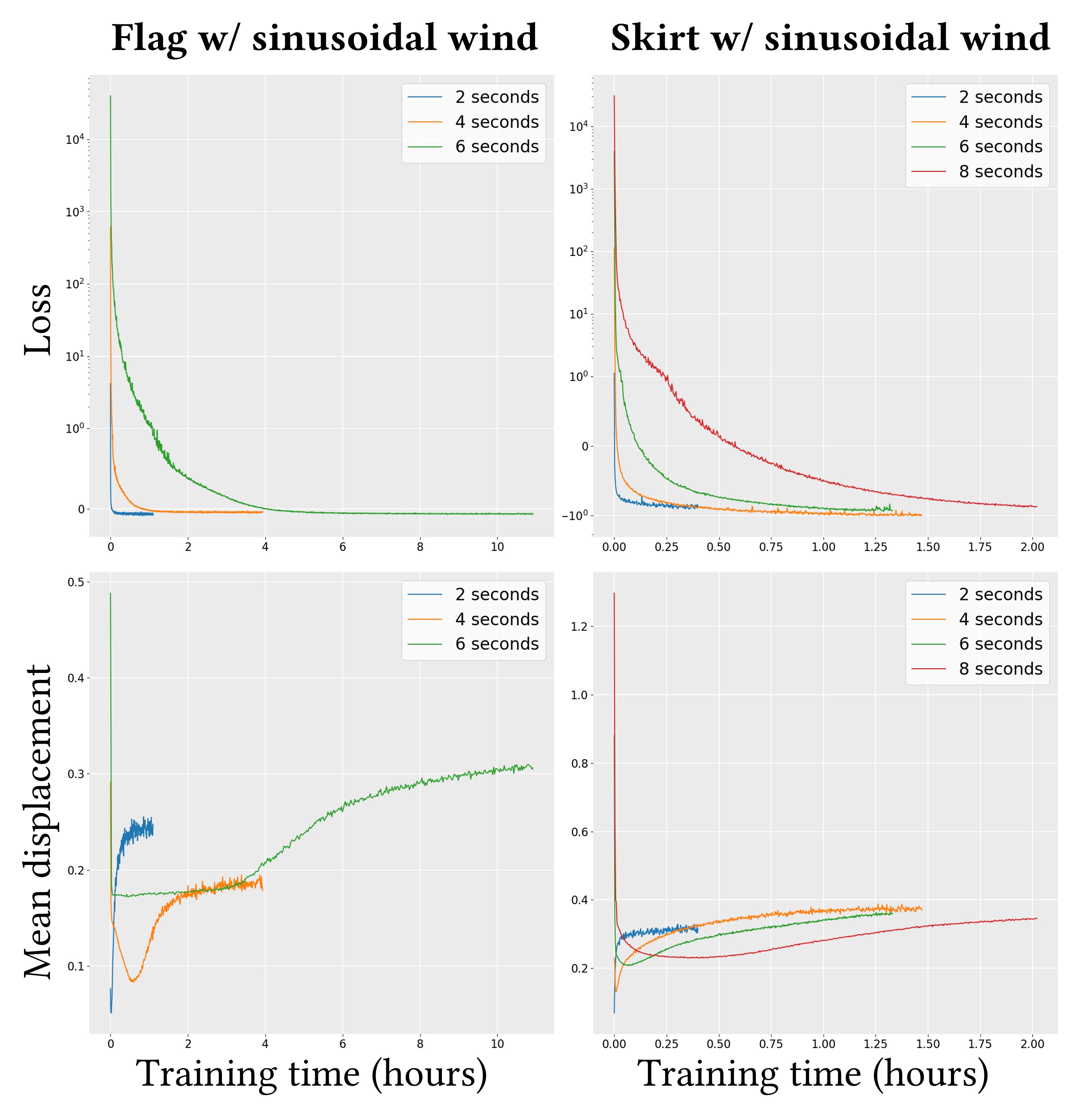
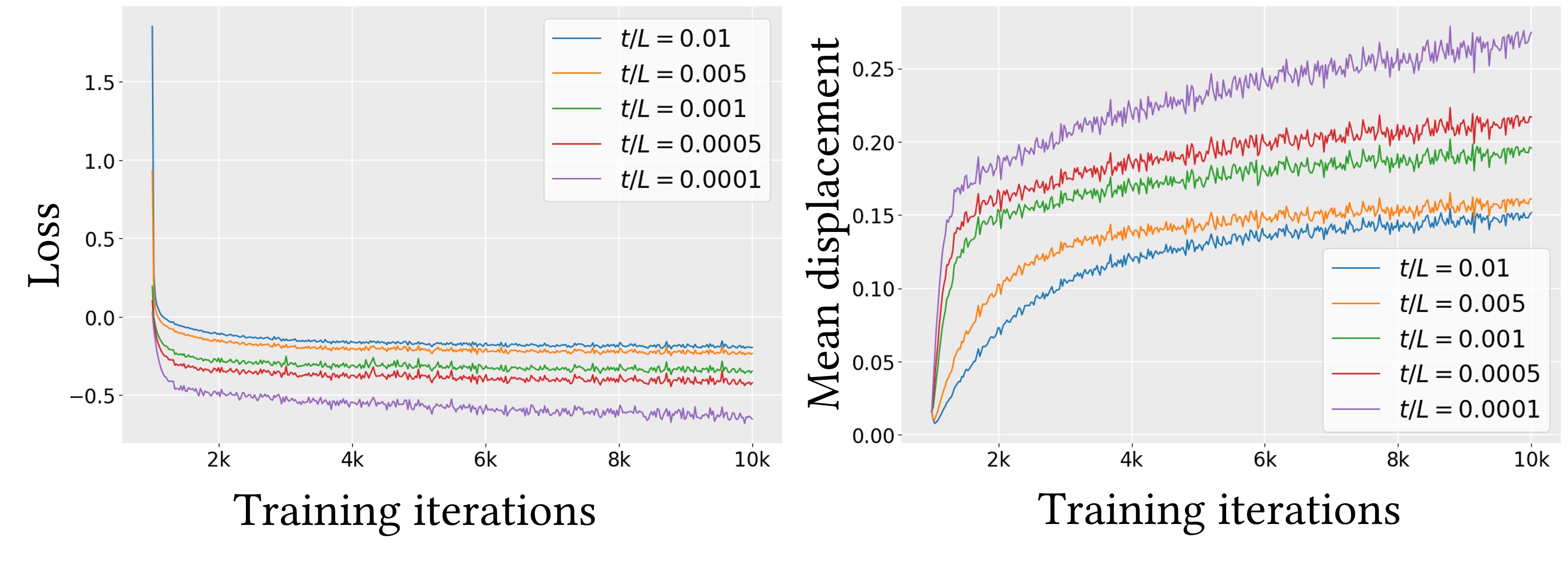
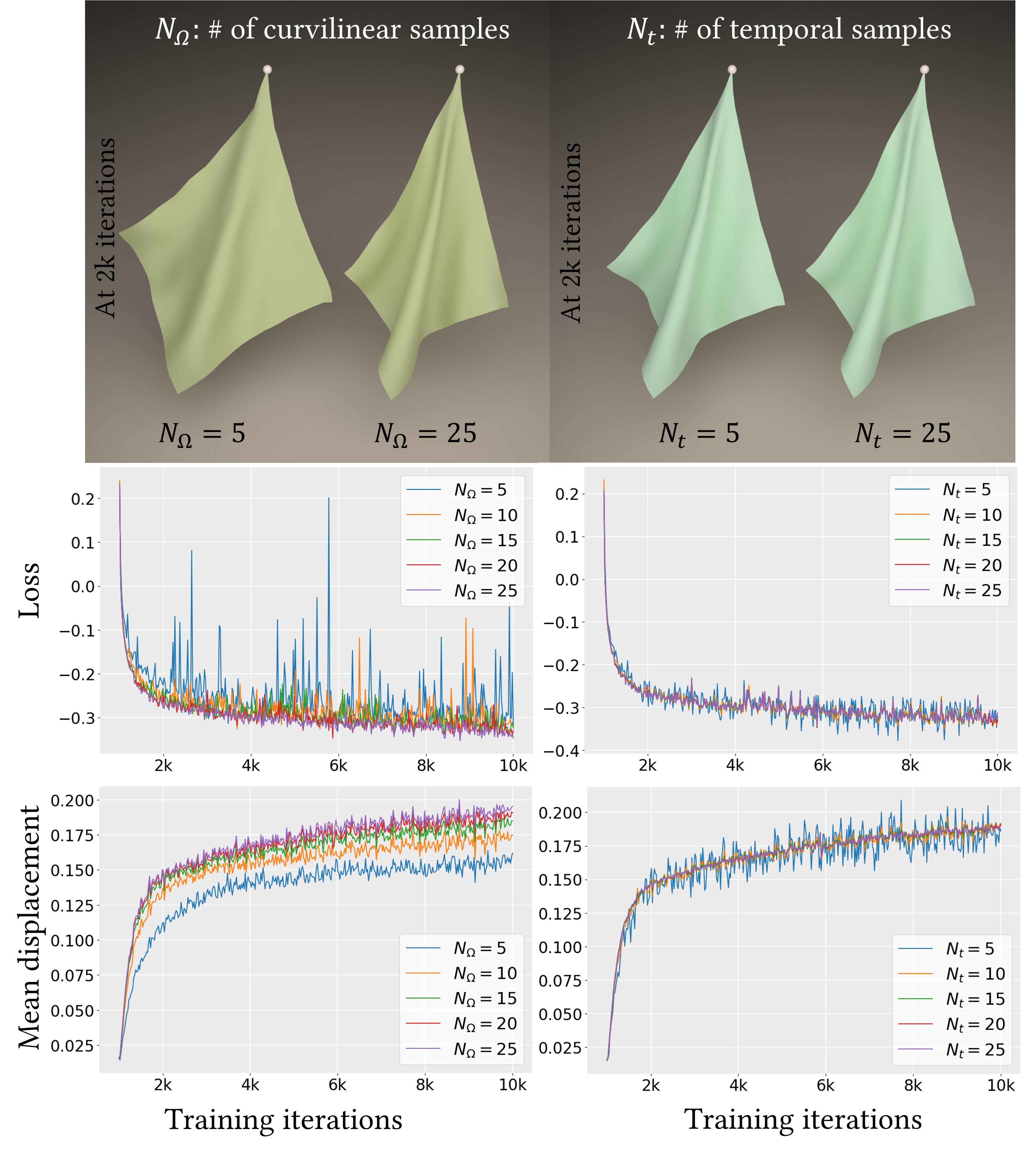
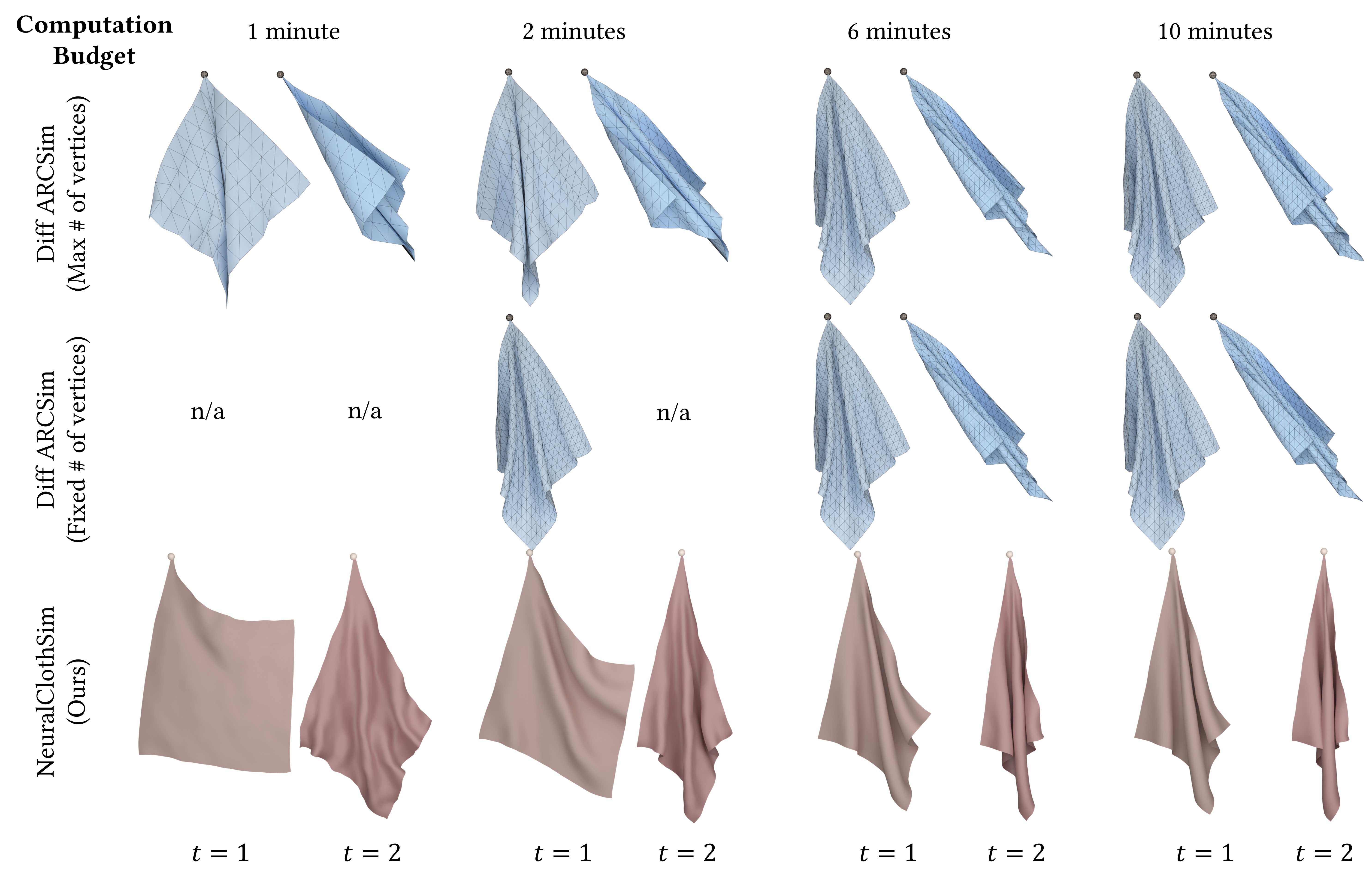
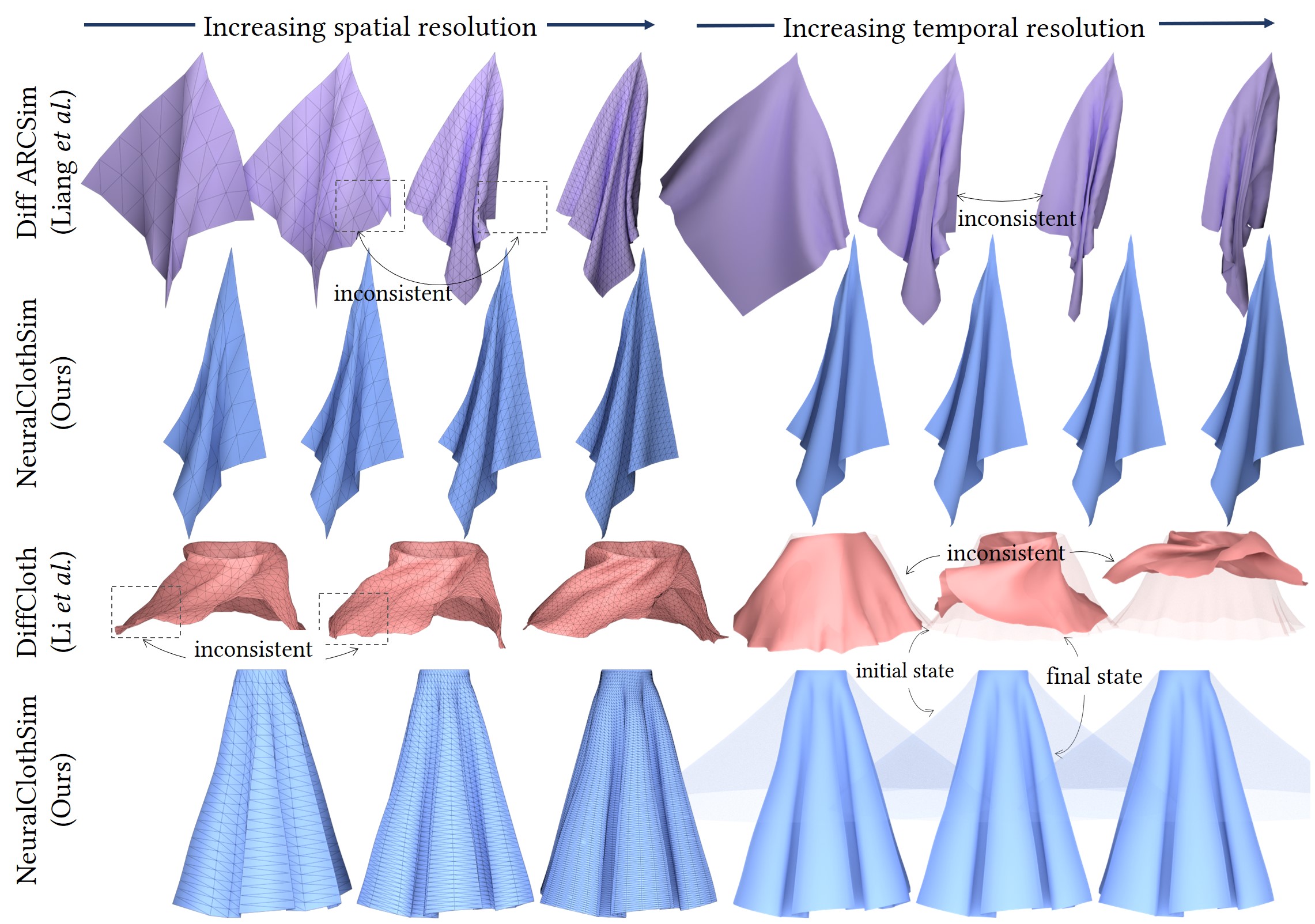
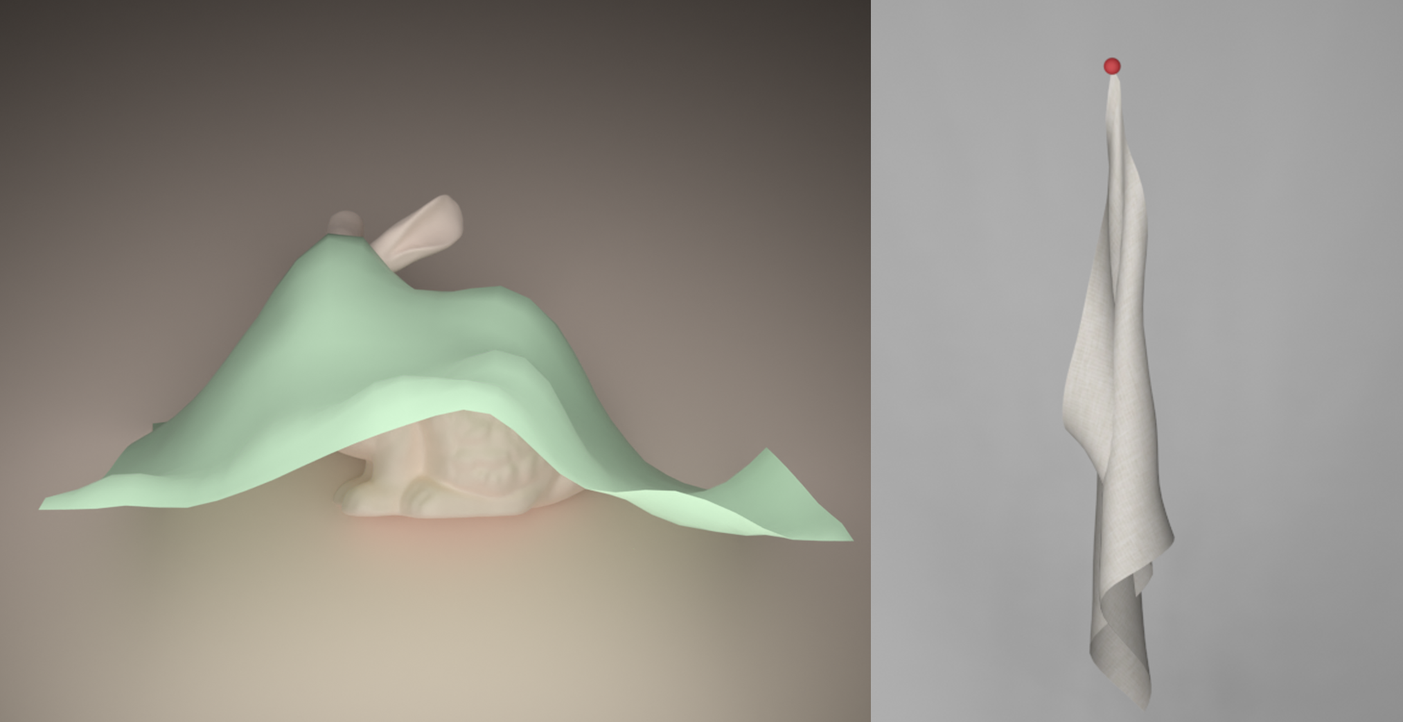
Appendix F Further Ablations

F.1. Boundary Constraints

We perform ablations on the Dirichlet and periodic boundary conditions. We try a soft constraint variation, in which we impose the boundary condition as a loss term in addition to the Kirchhoff-Love energy: This requires empirically determining the optimal loss weight, takes much longer to train and does not guarantee satisfying boundary constraints, as shown in Fig. II-(top). Our approach with hard constraints avoids all these problems. In the second example, we simulate the compression of a cylindrical sleeve as described in Sec. E.2. As seen in Fig. II-(bottom), at $\xi^{1}=\pi$, cylinder (a:) is disconnected if no constraint is specified; (b:) is connected with $\xi^{1}\mapsto\cos\xi^{1}$; (c:) fully models continuity and differentiability forming folds with $\xi^{1}\mapsto\{\cos\xi^{1},\sin\xi^{1}\}$.

F.2. Activation Function

Experimental results for a sleeve twist with different activation functions in the NDF network are shown in Fig. III. While ReLU lacks support for higher-order derivatives leading to artefacts, a network with GELU activation can only represent low-frequency deformations. Our usage of sine activation (Sitzmann et al., 2020) overcomes these limitations and successfully represents fine folds.

Appendix G Performance

The performance of a cloth simulator—such as the computation time and the scalability to long simulations—is a crucial aspect of its usability. This work focuses on the fundamental challenges of developing an implicit neural simulator with new characteristics. Our method does not outperform the classical simulators in all aspects as they are well-engineered and highly optimised. Next, we provide a detailed analysis of NeuralClothSim’s performance.

G.1. Runtime

NeuralClothSim encodes the spatio-temporal cloth simulation as an NDF, and, consequently, the bulk of computation time lies in the NDF training (i.e., optimisation of the network weights). At inference, extracting the simulated states from NDF as meshes or point clouds requires a single forward pass and is, therefore, fast. In Fig. IV, we provide a runtime analysis of three representative simulations (each of one-second duration) as a function of training time. On the left, we visualise the evolution of the last frame showing the refinement of the simulated state with increased training time. Before training, the simulation state is the sum of the reference state and random noisy output from NDF. Within a few minutes of training, NDF generates reasonable simulations, which then converge within 30 minutes to one hour; see our supplementary video for the evolution of simulation states over training iterations. On the top-right of Fig. IV, we plot loss values as a function of training time, which shows that our training is stable. As NeuralClothSim is an instance of a physics-informed neural network with a physics loss only (but no data term), the loss is not expected to converge to zero. We monitor the mean NDF over all sampled spatio-temporal points (Fig. IV-(bottom right)) as an additional cue on the simulation refinement. Along with the loss, saturation in mean NDF can be used as a stopping criterion. Note that all our experiments are carried out on a single NVIDIA Quadro RTX 8000 GPU.

Similar to classical methods (Choi and Ko, 2005), simulation with our approach is not unique, as bifurcation due to buckling can lead to solutions with different folds and wrinkles. Among them, the selection of the simulation outcome depends on the NDF convergence. Specifically, the randomness in training samples and weight initialisation introduces desirable optimisation path variations. In all cases, we observe NDF training to be numerically stable.

G.2. Scalability

Next, we study the performance of our method in simulating longer sequences. We consider two scenarios: (1) a flag waving in the wind, and (2) a skirt moving under gravity and wind. Both simulations are subject to time-dependent sinusoidal wind force defined as $\mathbf{f}=0.5\sin\left(\omega t+\phi\right)\mathbf{d}^{\top}$. We set $\omega=2,\phi=1$ and the amplitude as $\mathbf{d}=[0.6,-0.4,0.3]^{\top}$ and $\mathbf{d}=[-0.7,0.6,0]^{\top}$ for flag and skirt, respectively. Both scenes are simulated for varying lengths (two, four, six and eight seconds) and their convergence plots are shown in Fig. V. The longest simulation sequences are visualised in the supplementary video. All simulations are performed with the same NDF network capacity (five hidden layers and $512$ units), except for the flag simulation of six seconds, for which we increased the number of layers to eight. We observe that, unlike FEM-based methods, learning longer-term behaviour is challenging for our method, as NeuralClothSim needs to solve a 4D optimisation over a large time domain. As seen in Fig. V, the initial loss is accordingly rather high for longer sequences (note the $\log$ scale of $y$-axis).

Appendix H Robustness

We next investigate if the NDF training policy is robust to varying shell thickness and the varying number of input samples.

H.1. Thinness Limit

NeuralClothSim considers thin shells with a thickness-to-width ratio $<0.01$. Hence, transverse shear strain is negligible and the Kirchhoff-Love theory holds. Bastek and Kochmann (2023) noted that MLP-based representations struggle with convergence at the limit of the shell thinness. They attribute this to the imbalance of membrane vs bending energies in the loss function for very small thickness values. Considering the similarity of our hyper-elastic energy formulation to theirs, we analyse the effect of thinness to find out if it is a potential issue.

Particularly, we simulate napkins under gravity with thickness-to-length ($t/L$) ratios varying from $10^{-2}$ to $10^{-4}$. In Fig. VI, we plot the losses and mean NDF displacements over training iterations for varying thickness values: Although the training is stable in all cases, the simulation of thinner shells takes longer to converge. Note that thinner clothes are more compliant to stretching and bending, leading to higher deformations as seen in Fig.1-(main matter). We remark that the ill-posedness of the loss function arises from the linear elasticity and future methods could integrate non-linear, data-driven material models that are better suited for clothes (e.g., (Wang et al., 2011)).

H.2. Sampling Strategy

Next, we study the influence of the number of training points on the performance of our method. Input samples to NDF include curvilinear $N_{\Omega}$ and temporal stratified $N_{t}$ coordinates over which the loss is computed at each training iteration. For a napkin of size $\Omega=[0,1]^{2}$, we simulate for $t\in[0,1]$ by training NDF for 10k iterations with number of sampling points $N_{\Omega},N_{t}\in\{5,10,15,20,25\}$. Computation times for all experiments are comparable (and slightly higher for the higher number of samples) as they share the GPU memory and are processed in parallel. Fig. VII shows the qualitative and quantitative performance. We observe that higher $N_{\Omega}$ leads to faster learning, as seen in the qualitative result in the top row and the mean displacement plot in the bottom row. Furthermore, it leads to stable optimisation, as seen in the loss plot. Interestingly, although it makes the training behaviour less noisy, increasing $N_{t}$ does not lead to faster optimisation (Fig. VII-(right column)). Future work could explore advanced sampling techniques for improved performance.

Appendix I Additional Comparisons

I.1. Runtime

We compare the runtime of our method to those of the FEM-based simulator DiffARCSim (Liang et al., 2019; Narain et al., 2012). Since our approach does not support collisions, we turn off collision handling in DiffARCSim due to the computational overheads for a fair comparison. We simulate a napkin sequence for two seconds and the results are visualised in Fig. VIII. For the same computation budget (runtime), we show two simulated states (at $\qty{1}{s}$ and $\qty{2}{s}$ denoted as t = 1 and t = 2 in the figure) for both methods. Note that DiffARCSim integrates forward in time, solving for a 3D deformation field at each time step, in contrast to ours which optimises for the 4D spatio-temporal NDF. Therefore, we present two sets of results for DiffARCSim, i.e., simulated states for the given computational budget 1) with maximum mesh resolution (Fig. VIII-(top row)) and 2) with fixed mesh resolution (Fig. VIII-(middle row)). We notice that both methods refine the simulated states with increased runtime. With decreasing computational budget, DiffARCSim produces converged simulated states of the cloth at low resolutions or only early frames at high resolutions. On the other hand, NeuralClothSim offers partially converged simulations at arbitrary resolutions as the runtime decreases. However, our approach is not yet scalable to longer-duration simulations as described in Sec. G.2, in contrast to DiffARCSim.

I.2. Multi-Resolution Consistency

Next, we show the comparison of NeuralClothSim to DiffARCSim, and DiffCloth (Li et al., 2022) in terms of the multi-resolution simulation consistency. We simulate 1) a napkin with a fixed corner under gravity, with our approach and ARCsim (Fig. IX, top two rows) and 2) a twisting and twirling motion of the skirt with our approach and DiffCloth (Fig. IX, two bottom rows). The compared simulators operate on meshes of pre-defined resolution (as provided initially). Hence, they need to run from scratch for different mesh resolutions and frame rates, and the simulation outcome is not guaranteed to be the same across these runs under different discretisations. Thus, increasing (or decreasing) spatial or temporal resolution can result in different folds or wrinkles instead of refining simulations at coarser resolutions. Unlike DiffARCSim and DiffCloth, our method provides consistent simulation at arbitrary resolutions. The same 3D points remain unaltered in meshes extracted from NDF at different resolutions and the instantaneous simulation outcome is identical irrespective of the temporal query parameters (frame rate). We emphasise that we do not claim consistent refinement as a function of runtime but rather a consistent simulation with respect to spatio-temporal sampling (at a given computational budget). This means that both converged or partially converged NDF provide a consistent simulation when queried at different spatio-temporal inputs.

Our comparison deviates from the literature, as the primary reason for using different spatio-temporal resolutions is to adjust runtime and memory usage. For example, the recent method of (Zhang et al., 2022) produces artefact-free previewing geometries (at various approximation levels) by biasing their solutions with shell forces and energies evaluated on the finest-level model. This approach offers a trade-off between runtime vs resolution while maintaining simulation consistency. In contrast, with NeuralClothSim, simulation is consistent at arbitrary resolutions at any moment during the NDF training, which, we believe, is still beneficial for many downstream tasks. Of course, ARCSim and DiffCloth also support very high resolutions and small temporal step sizes, which eventually enables browsing the simulations at different frame rates and mesh resolutions (while maintaining mesh consistency across the levels); however, at the cost of high memory consumption. Moreover, in their case, methods for inverse problems that estimate the simulation parameters from simulated states cannot use adaptive (e.g., coarse-to-fine and importance) sampling. In contrast, our continuous formulation offers clear advantages in this regard.

Appendix J Limitations and Future Research

NeuralClothSim is the first step towards a neural implicit cloth simulation. Currently, our approach does not handle collisions, contacts and frictions, nor do we model effects such as damping. In a preliminary experiment, we model collisions with external objects following earlier neural methods (Santesteban et al., 2022; Bertiche et al., 2022), i.e., we define an additional loss term $\mathcal{L}_{\mathrm{collision}}(\Theta)$ that penalises collisions, leading to:

(75) $$\begin{split}\mathcal{L}&=\mathcal{L}_{\mathrm{physics}}(\Theta)+\lambda\mathcal{L}_{\mathrm{collision}}(\Theta),\;\text{with}\\ \mathcal{L}_{\mathrm{collision}}(\Theta)&=\frac{|\Omega|}{N_{\Omega}N_{t}}\sum_{i=1}^{N_{\Omega}}\sum_{j=1}^{N_{t}}\max(\epsilon-\operatorname{SDF}(\mathbf{x}(\boldsymbol{\xi}_{i},t_{j};\Theta)),0),\end{split}$$

where $\operatorname{SDF}(\mathbf{x})$ is the signed distance to the object, $\epsilon$ is a small safety margin between cloth and object to ensure robustness, $\lambda$ is the weight for the collision term, and $\mathcal{L}_{\mathrm{physics}}(\Theta)$ is our main thin-shell loss in Eq. (35)-(main matter). We set $\lambda=1000$, $\epsilon=0.001$, and use a pre-trained SDF network encoding signed distance function. Specifically, we employ the method of Sitzmann et al. (2020) to fit an SDF network on an oriented point cloud, where an Eikonal regularisation is used in addition to the SDF and normal loss. Fig. X-(left) visualises a simulation result for a piece of cloth falling on the Stanford bunny after one second; see our supplementary video for the full simulation. We observe that the cloth coarsely respects the object contours, although constraints in Eq. (75) are soft and do not guarantee physically realistic deformations. Difficulties in training PINN with multiple loss terms were previously reported in the literature (Hao et al., 2022) and future research is necessary to further investigate collision handling in the context of NDFs.

Next, NeuralClothSim is differentiable by construction and we believe it will be useful for inverse problems such as non-rigid 3D surface capture from single or multi-view videos. Moreover, NeuralClothSim may require carefully choosing scenario-specific boundary constraints, and the periodic boundary formulation helps mainly with simple geometries. Future work could also explore modelling different types of human clothing with the help of the proposed implicit neural framework.

References

- (1)
- Baraff and Witkin (1998) David Baraff and Andrew Witkin. 1998. Large Steps in Cloth Simulation. In Annual Conference on Computer Graphics and Interactive Techniques (SIGGRAPH ’98).
- Barr (1984) Alan H. Barr. 1984. Global and Local Deformations of Solid Primitives. In Annual Conference on Computer Graphics and Interactive Techniques (SIGGRAPH).
- Basar and Krätzig (2013) Yavuz Basar and Wilfried B Krätzig. 2013. Mechanik der Flächentragwerke: theorie, berechnungsmethoden, anwendungsbeispiele. Springer-Verlag.
- Bastek and Kochmann (2023) Jan-Hendrik Bastek and Dennis M Kochmann. 2023. Physics-Informed Neural Networks for shell structures. European Journal of Mechanics-A/Solids (2023).
- Behzadinasab et al. (2022) Masoud Behzadinasab, Mert Alaydin, Nathaniel Trask, and Yuri Bazilevs. 2022. A general-purpose, inelastic, rotation-free Kirchhoff–Love shell formulation for peridynamics. Computer Methods in Applied Mechanics and Engineering (2022).
- Belytschko et al. (1985) Ted Belytschko, Henryk Stolarski, Wing Kam Liu, Nicholas Carpenter, and Jame SJ Ong. 1985. Stress projection for membrane and shear locking in shell finite elements. Computer Methods in Applied Mechanics and Engineering (1985).
- Bender and Deul (2012) Jan Bender and Crispin Deul. 2012. Efficient Cloth Simulation Using an Adaptive Finite Element Method.. In VRIPHYS.
- Bertiche et al. (2021) Hugo Bertiche, Meysam Madadi, and Sergio Escalera. 2021. PBNS: physically based neural simulation for unsupervised garment pose space deformation. ACM Transactions on Graphics (TOG) (2021).
- Bertiche et al. (2022) Hugo Bertiche, Meysam Madadi, and Sergio Escalera. 2022. Neural Cloth Simulation. ACM Transactions on Graphics (TOG) (2022).
- Bridson et al. (2002) Robert Bridson, Ronald Fedkiw, and John Anderson. 2002. Robust treatment of collisions, contact and friction for cloth animation. In ACM Transactions on Graphics.
- Bridson et al. (2005) Robert Bridson, Sebastian Marino, and Ronald Fedkiw. 2005. Simulation of clothing with folds and wrinkles. In ACM SIGGRAPH 2005 Courses.
- Chen et al. (2023b) Honglin Chen, Rundi Wu, Eitan Grinspun, Changxi Zheng, and Peter Yichen Chen. 2023b. Implicit Neural Spatial Representations for Time-dependent PDEs. In International Conference on Machine Learning (ICML).
- Chen et al. (2018b) Hsiao-Yu Chen, Arnav Sastry, Wim M van Rees, and Etienne Vouga. 2018b. Physical simulation of environmentally induced thin shell deformation. ACM Transactions on Graphics (2018).
- Chen et al. (2023a) Peter Yichen Chen, Maurizio M Chiaramonte, Eitan Grinspun, and Kevin Carlberg. 2023a. Model reduction for the material point method via an implicit neural representation of the deformation map. J. Comput. Phys. (2023).
- Chen et al. (2022) Peter Yichen Chen, Jinxu Xiang, Dong Heon Cho, Yue Chang, GA Pershing, Henrique Teles Maia, Maurizio Chiaramonte, Kevin Carlberg, and Eitan Grinspun. 2022. CROM: Continuous reduced-order modeling of PDEs using implicit neural representations. arXiv preprint arXiv:2206.02607 (2022).
- Chen et al. (2018a) Ricky T. Q. Chen, Yulia Rubanova, Jesse Bettencourt, and David Duvenaud. 2018a. Neural Ordinary Differential Equations. Advances in Neural Information Processing Systems (NeurIPS) (2018).
- Choi and Ko (2005) Kwang-Jin Choi and Hyeong-Seok Ko. 2005. Stable but responsive cloth. In ACM SIGGRAPH 2005 Courses.
- Cirak and Ortiz (2001) Fehmi Cirak and Michael Ortiz. 2001. Fully C1-conforming subdivision elements for finite deformation thin-shell analysis. Internat. J. Numer. Methods Engrg. (2001).
- Cirak et al. (2000) Fehmi Cirak, Michael Ortiz, and Peter Schröder. 2000. Subdivision surfaces: a new paradigm for thin-shell finite-element analysis. Internat. J. Numer. Methods Engrg. (2000).
- Clyde et al. (2017) David Clyde, Joseph Teran, and Rasmus Tamstorf. 2017. Simulation of nonlinear Kirchhoff-Love thin shells using subdivision finite elements. In Proc. ACM SIGGRAPH / Eurographics Symposium on Computer Animation (SCA).
- Etzmuß et al. (2003) Olaf Etzmuß, Michael Keckeisen, and Wolfgang Straßer. 2003. A fast finite element solution for cloth modelling. In Proc. of The Pacific Conference on Computer Graphics and Applications.
- Green et al. (2002) Seth Green, George Turkiyyah, and Duane Storti. 2002. Subdivision-based multilevel methods for large scale engineering simulation of thin shells. In Proceedings of the seventh ACM symposium on Solid modeling and applications.
- Grinspun et al. (2006) Eitan Grinspun, Yotam Gingold, Jason Reisman, and Denis Zorin. 2006. Computing discrete shape operators on general meshes. In Computer Graphics Forum.
- Grinspun et al. (2003) Eitan Grinspun, Anil N Hirani, Mathieu Desbrun, and Peter Schröder. 2003. Discrete shells. In Proc. ACM SIGGRAPH / Eurographics Symposium on Computer Animation (SCA).
- Grinspun et al. (2002) Eitan Grinspun, Petr Krysl, and Peter Schröder. 2002. CHARMS: A simple framework for adaptive simulation. ACM Transactions on Graphics (2002).
- Gundogdu et al. (2019) Erhan Gundogdu, Victor Constantin, Amrollah Seifoddini, Minh Dang, Mathieu Salzmann, and Pascal Fua. 2019. Garnet: A two-stream network for fast and accurate 3d cloth draping. In International Conference on Computer Vision (ICCV).
- Guo et al. (2021) Hongwei Guo, Xiaoying Zhuang, and Timon Rabczuk. 2021. A deep collocation method for the bending analysis of Kirchhoff plate. arXiv preprint arXiv:2102.02617 (2021).
- Guo et al. (2018) Qi Guo, Xuchen Han, Chuyuan Fu, Theodore Gast, Rasmus Tamstorf, and Joseph Teran. 2018. A material point method for thin shells with frictional contact. ACM Transactions on Graphics (2018).
- Hao et al. (2022) Zhongkai Hao, Songming Liu, Yichi Zhang, Chengyang Ying, Yao Feng, Hang Su, and Jun Zhu. 2022. Physics-Informed Machine Learning: A Survey on Problems, Methods and Applications. arXiv preprint arXiv:2211.08064 (2022).
- Harmon et al. (2008) David Harmon, Etienne Vouga, Rasmus Tamstorf, and Eitan Grinspun. 2008. Robust treatment of simultaneous collisions. In ACM SIGGRAPH 2008 papers.
- Hendrycks and Gimpel (2016) Dan Hendrycks and Kevin Gimpel. 2016. Gaussian error linear units (gelus). arXiv preprint arXiv:1606.08415 (2016).
- Kairanda et al. (2022) Navami Kairanda, Edith Tretschk, Mohamed Elgharib, Christian Theobalt, and Vladislav Golyanik. 2022. f-SfT: Shape-From-Template With a Physics-Based Deformation Model. In Computer Vision and Pattern Recognition (CVPR).
- Kiendl et al. (2009) J. Kiendl, K.-U. Bletzinger, J. Linhard, and R. Wüchner. 2009. Isogeometric shell analysis with Kirchhoff–Love elements. Computer Methods in Applied Mechanics and Engineering (2009).
- Kiendl et al. (2015) Josef Kiendl, Ming-Chen Hsu, Michael CH Wu, and Alessandro Reali. 2015. Isogeometric Kirchhoff–Love shell formulations for general hyperelastic materials. Computer Methods in Applied Mechanics and Engineering (2015).
- Kingma and Ba (2014) Diederik P Kingma and Jimmy Ba. 2014. Adam: A method for stochastic optimization. arXiv preprint arXiv:1412.6980 (2014).
- Kopanicakova et al. (2019) Alena Kopanicakova, Rolf Krause, and Rasmus Tamstorf. 2019. Subdivision-based nonlinear multiscale cloth simulation. SIAM Journal on Scientific Computing (2019).
- Lähner et al. (2018) Zorah Lähner, Daniel Cremers, and Tony Tung. 2018. DeepWrinkles: Accurate and Realistic Clothing Modeling. In European Conference on Computer Vision (ECCV).
- Li et al. (2020) Cheng Li, Min Tang, Ruofeng Tong, Ming Cai, Jieyi Zhao, and Dinesh Manocha. 2020. P-cloth: interactive complex cloth simulation on multi-GPU systems using dynamic matrix assembly and pipelined implicit integrators. ACM Transactions on Graphics (2020).
- Li et al. (2018) Jie Li, Gilles Daviet, Rahul Narain, Florence Bertails-Descoubes, Matthew Overby, George E Brown, and Laurence Boissieux. 2018. An implicit frictional contact solver for adaptive cloth simulation. ACM Transactions on Graphics (2018).
- Li et al. (2022) Yifei Li, Tao Du, Kui Wu, Jie Xu, and Wojciech Matusik. 2022. DiffCloth: Differentiable cloth simulation with dry frictional contact. ACM Transactions on Graphics (2022).
- Li et al. (2021) Yue Li, Marc Habermann, Bernhard Thomaszewski, Stelian Coros, Thabo Beeler, and Christian Theobalt. 2021. Deep Physics-aware Inference of Cloth Deformation for Monocular Human Performance Capture. In International Conference on 3D Vision (3DV).
- Liang et al. (2019) Junbang Liang, Ming Lin, and Vladlen Koltun. 2019. Differentiable Cloth Simulation for Inverse Problems. In Advances in Neural Information Processing Systems (NeurIPS).
- Love (2013) Augustus Edward Hough Love. 2013. A treatise on the mathematical theory of elasticity. Cambridge university press.
- Lu and Zheng (2014) Jia Lu and Chao Zheng. 2014. Dynamic cloth simulation by isogeometric analysis. Computer Methods in Applied Mechanics and Engineering (2014).
- Lu et al. (2021) Lu Lu, Raphael Pestourie, Wenjie Yao, Zhicheng Wang, Francesc Verdugo, and Steven G Johnson. 2021. Physics-informed neural networks with hard constraints for inverse design. SIAM Journal on Scientific Computing (2021).
- Ly et al. (2020) Mickaël Ly, Jean Jouve, Laurence Boissieux, and Florence Bertails-Descoubes. 2020. Projective dynamics with dry frictional contact. ACM Transactions on Graphics (TOG) (2020).
- Martin et al. (2010) Sebastian Martin, Peter Kaufmann, Mario Botsch, Eitan Grinspun, and Markus Gross. 2010. Unified simulation of elastic rods, shells, and solids. ACM Transactions on Graphics (2010).
- Mildenhall et al. (2020) Ben Mildenhall, Pratul P Srinivasan, Matthew Tancik, Jonathan T Barron, Ravi Ramamoorthi, and Ren Ng. 2020. Nerf: Representing scenes as neural radiance fields for view synthesis. In European Conference on Computer Vision (ECCV).
- Müller et al. (2022) Thomas Müller, Alex Evans, Christoph Schied, and Alexander Keller. 2022. Instant neural graphics primitives with a multiresolution hash encoding. ACM Transactions on Graphics (2022).
- Naghdi (1973) Paul Mansour Naghdi. 1973. The theory of shells and plates. In Linear theories of elasticity and thermoelasticity: linear and nonlinear theories of rods, plates, and shells. Springer, 425–640.
- Narain et al. (2012) Rahul Narain, Armin Samii, and James F O’brien. 2012. Adaptive anisotropic remeshing for cloth simulation. ACM Transactions on Graphics (2012).
- Oechsle et al. (2021) Michael Oechsle, Songyou Peng, and Andreas Geiger. 2021. UNISURF: Unifying Neural Implicit Surfaces and Radiance Fields for Multi-View Reconstruction. In International Conference on Computer Vision (ICCV).
- Oh et al. (2018) Young Jin Oh, Tae Min Lee, and In-Kwon Lee. 2018. Hierarchical cloth simulation using deep neural networks. In Proceedings of Computer Graphics International.
- Otaduy et al. (2009) Miguel A Otaduy, Rasmus Tamstorf, Denis Steinemann, and Markus Gross. 2009. Implicit contact handling for deformable objects. In Compututer Graphics Forum.
- Park et al. (2019) Jeong Joon Park, Peter Florence, Julian Straub, Richard Newcombe, and Steven Lovegrove. 2019. DeepSDF: Learning Continuous Signed Distance Functions for Shape Representation. In Computer Vision and Pattern Recognition (CVPR).
- Park et al. (2021) Keunhong Park, Utkarsh Sinha, Jonathan T. Barron, Sofien Bouaziz, Dan B Goldman, Steven M. Seitz, and Ricardo Martin-Brualla. 2021. Nerfies: Deformable Neural Radiance Fields. International Conference on Computer Vision (ICCV) (2021).
- Paszke et al. (2019) Adam Paszke, Sam Gross, Francisco Massa, Adam Lerer, James Bradbury, Gregory Chanan, Trevor Killeen, Zeming Lin, Natalia Gimelshein, Luca Antiga, et al. 2019. Pytorch: An imperative style, high-performance deep learning library. Advances in Neural Information Processing Systems (NeurIPS) (2019).
- Pfaff et al. (2021) Tobias Pfaff, Meire Fortunato, Alvaro Sanchez-Gonzalez, and Peter Battaglia. 2021. Learning Mesh-Based Simulation with Graph Networks. In International Conference on Learning Representations (ICLR).
- Pumarola et al. (2020) Albert Pumarola, Enric Corona, Gerard Pons-Moll, and Francesc Moreno-Noguer. 2020. D-NeRF: Neural Radiance Fields for Dynamic Scenes. In Computer Vision and Pattern Recognition (CVPR).
- Raissi et al. (2019) Maziar Raissi, Paris Perdikaris, and George E Karniadakis. 2019. Physics-informed neural networks: A deep learning framework for solving forward and inverse problems involving nonlinear partial differential equations. J. Comput. Phys. (2019).
- Santesteban et al. (2022) Igor Santesteban, Miguel A Otaduy, and Dan Casas. 2022. SNUG: Self-Supervised Neural Dynamic Garments. Computer Vision and Pattern Recognition (CVPR) (2022).
- Schöllhammer and Fries (2019) Daniel Schöllhammer and Thomas-Peter Fries. 2019. Kirchhoff–Love shell theory based on tangential differential calculus. Computational mechanics (2019).
- Scordelis and Lo (1964) AC Scordelis and KS Lo. 1964. Computer analysis of cylindrical shells. In Journal Proceedings.
- Simo and Fox (1989) Juan C Simo and David D Fox. 1989. On a stress resultant geometrically exact shell model. Part I: Formulation and optimal parametrization. Computer Methods in Applied Mechanics and Engineering (1989).
- Sitzmann et al. (2020) Vincent Sitzmann, Julien Martel, Alexander Bergman, David Lindell, and Gordon Wetzstein. 2020. Implicit neural representations with periodic activation functions. In Advances in Neural Information Processing Systems (NeurIPS).
- Tang et al. (2018a) Min Tang, Zhongyuan Liu, Ruofeng Tong, and Dinesh Manocha. 2018a. PSCC: Parallel self-collision culling with spatial hashing on GPUs. Proceedings of the ACM on Computer Graphics and Interactive Techniques (2018).
- Tang et al. (2018b) Min Tang, Tongtong Wang, Zhongyuan Liu, Ruofeng Tong, and Dinesh Manocha. 2018b. I-Cloth: Incremental collision handling for GPU-based interactive cloth simulation. ACM Transactions on Graphics (2018).
- Terzopoulos et al. (1987) Demetri Terzopoulos, John Platt, Alan Barr, and Kurt Fleischer. 1987. Elastically Deformable Models. SIGGRAPH Comput. Graph. (1987).
- Thomaszewski et al. (2006) Bernhard Thomaszewski, Markus Wacker, and Wolfgang Straßer. 2006. A consistent bending model for cloth simulation with corotational subdivision finite elements. In Proc. ACM SIGGRAPH / Eurographics Symposium on Computer Animation (SCA).
- Timoshenko et al. (1959) Stephen Timoshenko, Sergius Woinowsky-Krieger, et al. 1959. Theory of plates and shells. Vol. 2. McGraw-hill New York.
- Tretschk et al. (2021) Edgar Tretschk, Ayush Tewari, Vladislav Golyanik, Michael Zollhöfer, Christoph Lassner, and Christian Theobalt. 2021. Non-Rigid Neural Radiance Fields: Reconstruction and Novel View Synthesis of a Dynamic Scene From Monocular Video. In IEEE International Conference on Computer Vision (ICCV). IEEE.
- Volino and Thalmann (2000) Pascal Volino and N Magnenat Thalmann. 2000. Implementing fast cloth simulation with collision response. In Proceedings Computer Graphics International 2000.
- Wang (2021) Huamin Wang. 2021. GPU-based simulation of cloth wrinkles at submillimeter levels. ACM Transactions on Graphics (2021).
- Wang et al. (2011) Huamin Wang, James F O’Brien, and Ravi Ramamoorthi. 2011. Data-driven elastic models for cloth: modeling and measurement. ACM Transactions on Graphics (2011).
- Wang et al. (2021) Peng Wang, Lingjie Liu, Yuan Liu, Christian Theobalt, Taku Komura, and Wenping Wang. 2021. NeuS: Learning Neural Implicit Surfaces by Volume Rendering for Multi-view Reconstruction. NeurIPS (2021).
- Wempner and Talaslidis (2003) Gerald Wempner and Demosthenes Talaslidis. 2003. Mechanics of solids and shells. CRC, Boca Raton (2003).
- Xie et al. (2022) Yiheng Xie, Towaki Takikawa, Shunsuke Saito, Or Litany, Shiqin Yan, Numair Khan, Federico Tombari, James Tompkin, Vincent Sitzmann, and Srinath Sridhar. 2022. Neural fields in visual computing and beyond. In Computer Graphics Forum (Eurographics State of the Art Reports).
- Yang et al. (2021) Guandao Yang, Serge Belongie, Bharath Hariharan, and Vladlen Koltun. 2021. Geometry processing with neural fields. Advances in Neural Information Processing Systems (NeurIPS) (2021).
- Yoshimura (1955) Yoshimaru Yoshimura. 1955. On the Mechanism of Buckling of a Circular Cylindrical Shell Under Axial Compression. National Advisory Commitee for Aeronautics (1955).
- Zhang et al. (2022) Jiayi Eris Zhang, Jérémie Dumas, Yun Fei, Alec Jacobson, Doug L James, and Danny M Kaufman. 2022. Progressive Simulation for Cloth Quasistatics. ACM Transactions on Graphics (2022).