POCO: 3D Pose and Shape Estimation with Confidence

Abstract

The regression of 3D Human Pose and Shape (HPS) from an image is becoming increasingly accurate. This makes the results useful for downstream tasks like human action recognition or 3D graphics. Yet, no regressor is perfect, and accuracy can be affected by ambiguous image evidence or by poses and appearance that are unseen during training. Most current HPS regressors, however, do not report the confidence of their outputs, meaning that downstream tasks cannot differentiate accurate estimates from inaccurate ones. To address this, we develop POCO, a novel framework for training HPS regressors to estimate not only a 3D human body, but also their confidence, in a single feed-forward pass. Specifically, POCO estimates both the 3D body pose and a per-sample variance. The key idea is to introduce a Dual Conditioning Strategy (DCS) for regressing uncertainty that is highly correlated to pose reconstruction quality. The POCO framework can be applied to any HPS regressor and here we evaluate it by modifying HMR, PARE, and CLIFF. In all cases, training the network to reason about uncertainty helps it learn to more accurately estimate 3D pose. While this was not our goal, the improvement is modest but consistent. Our main motivation is to provide uncertainty estimates for downstream tasks; we demonstrate this in two ways: (1) We use the confidence estimates to bootstrap HPS training. Given unlabeled image data, we take the confident estimates of a POCO-trained regressor as pseudo ground truth. Retraining with this automatically-curated data improves accuracy. (2) We exploit uncertainty in video pose estimation by automatically identifying uncertain frames (e.g. due to occlusion) and “inpainting” these from confident frames. Code and models will be available for research at https://poco.is.tue.mpg.de.

Figure 1: Regressing 3D humans and confidence. Most existing methods that regress 3D Human Pose and Shape (HPS) do not report their confidence (or uncertainty). An estimate of confidence, however, is needed by methods that “consume” the results of HPS. Even the best HPS methods struggle when the image evidence is weak or ambiguous. Our framework, POCO, extends existing HPS regressors to also estimate uncertainty in a single forward pass. The confidence (color-coded on the body) is correlated with the pose quality.

1 Introduction

To reconstruct human actions in everyday environments we need to estimate 3D Human Pose and Shape (HPS) from images and videos. However, 3D inference from 2D images is highly ill-posed due to depth ambiguities, occlusion, unusual clothing, and motion blur. Not surprisingly, even the best HPS methods make mistakes. The problem is that they do not know it and neither do downstream tasks. HPS is not an end goal but, rather, an intermediate task that produces output that is consumed by downstream tasks like human behavior understanding or 3D graphics applications. Downstream tasks need to know when the results of an HPS method are accurate or not. Consequently, these methods should output a uncertainty (or confidence) value that is correlated with the HPS quality.

One approach to dealing with uncertainty is to output multiple bodies [3], but this still does not provide an explicit measure of uncertainty. There are several notable exceptions that estimate a distribution over body parameters [30, 51, 34]; sampling from this distribution generates multiple plausible bodies. For example, Sengupta et al. [51] compute uncertainty by drawing samples from a distribution over bodies and computing the standard deviation of the samples. While a valid approach, it has two drawbacks: (1) it is slow, since it requires multiple forward network passes to generate samples, and (2) it trades off accuracy for speed; the more the samples, the higher the accuracy, but the more computation is required. Instead, we propose an approach that infers uncertainty directly in a single network pass by training the network to output both the body parameters and the uncertainty. Note that we achieve this without any explicit supervision of the uncertainty.

We draw inspiration from Kendal et al. [22] who estimate uncertainty for semantic segmentation; they model the error of inferred segmentations using a base density function (bDF); they use a Gaussian distribution for this. Then, they infer a per-sample scale (i.e., uncertainty) using a scale network to refine this function and model a per-sample likelihood.

A Gaussian distribution is common for modeling sample error. However, recent work [35, 51, 52, 72] shows that a more complex distribution like a normalizing flow [7] is needed when modeling human poses, e.g., RLE [35] does so for modelling the error of 3D body joints.

Methods that directly estimate uncertainty [35, 22] usually have two components - a base density function and a scale network to refine the bDF. Kendal et al. [22] and RLE [35] use an unconditional bDF and only use image-features for the scale network. An unconditional bDF, shared among all samples, is reasonable if all samples share a similar distribution. However, this assumption breaks when using multiple datasets, which are needed to train robust 3D HPS models. Similarly, using only image features to infer a per-sample scale (i.e., uncertainty) does not consider the pose plausibility for the given image evidence.

We address these issues with POCO (“POse and shape estimation with COnfidence”), a novel framework that can be applied to common HPS methods, extending them to estimate uncertainty. In a single feed-forward pass, POCO directly infers both SMPL [40] body parameters and its regression uncertainty which is highly correlated to reconstruction quality; see POCO: 3D Pose and Shape Estimation with Confidence. The key novelty of our framework is a Dual Conditioning Strategy (DCS) which augments the bDF and scale network as described below:

(1) Image-conditioned bDF: In contrast to prior work, POCO models the bDF of the inferred pose error with a conditional vector (Cond-bDF). A naive condition would be a one-hot encoding of the data source. However, rich datasets contain images that are not necessarily drawn from a single distribution. Therefore, we use image features as conditioning, making training more scalable and possible on arbitrarily complex collections of images.

(2) Pose-conditioned scale: Previous methods infer a scale (i.e., uncertainty) value that refines the bDF for each image, using an MLP that takes image features as input. We go further to also condition the MLP on the regressed SMPL pose (“Cond-Scale”). We experimentally show that this improves pose reconstruction and helps estimate uncertainty based on pose plausibility for given image evidence.

Our formulation can be included in the loss function of existing HPS regressors. We show this by modifying HMR [19], PARE [26], and CLIFF [37] to also output uncertainty. A key observation is that this change uniformly improves the accuracy of these methods. That is, requiring the network to also estimate uncertainty helps it learn to better estimate pose and shape. While the accuracy improvement is modest, the important point is that one can apply POCO to existing regressors with no downside; i.e., one gets uncertainty estimates “for free.”

We perform qualitative evaluation on in-the-wild data and quantitative evaluation on 3DPW [59] and 3DOH [75]. We train all methods (HMR, PARE, CLIFF) and their POCO versions on the same data and show a quantitative improvement in accuracy in all cases. We also compare these POCO formulations to state-of-the-art (SOTA) HPS methods that model uncertainty and show higher correlation of uncertainty and pose error. Ablation studies show the efficacy of POCO’s novel contributions.

While improved pose accuracy is a welcome byproduct, our main goal is to exploit uncertainty estimates in downstream tasks. We demonstrate this in two practical tasks.

(1) HPS self-improvement: We show that HPS models can self-improve by leveraging uncertainty estimates to automatically bootstrap training. Specifically, we apply an HPS regressor trained with POCO on in-the-wild videos for which there is no ground truth. Normally such data would not be useful for training. We then take pairs of images and SMPL parameters that have high confidence and treat them as pseudo ground-truth training samples. We finally re-train the regressor on an enriched dataset that includes the pseudo ground truth and show that this improves accuracy. This works with all three HPS regressors that we evaluated.

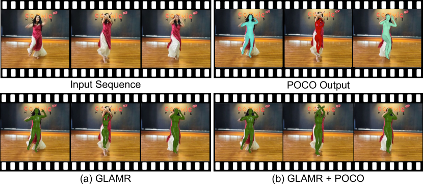
(2) HPS from video: In complex videos, single-frame HPS regressors make errors on challenging frames. We exploit the estimated uncertainty to automatically detect frames where the SMPL estimates may be inaccurate. We then remove these uncertain estimates and infill the corresponding frames following GLAMR [70]. This approach uses highly-confident bodies and knowledge of human motion to produce more plausible 4D HPS results.

In summary, we make the following key contributions: (1) We are the first to demonstrate a general uncertainty framework, POCO, that can be applied to common HPS methods for estimating uncertainty in a single forward pass. (2) We introduce a Dual Conditioning Strategy (DCS) that helps regress uncertainty that is highly correlated to pose reconstruction quality and improves the accuracy of exisiting HPS regressors. (3) We show that the uncertainty estimate given by POCO can be used for two practical downstream tasks. Our framework gives existing methods a simple way to estimate uncertainty with no downside, and it even improves performance. We believe this will make HPS results more useful for downstream tasks. Our models and code will be available.

2 Related Work

2.1 Deterministic HPS Estimation

Optimization-based methods: Such methods fit a parametric model [2, 40, 48, 67, 17] to cues extracted from images, such as keypoints [5, 65, 67], silhouettes [45, 14], part segmentation masks [33], or part orientation fields [65].

Learning-based methods: Datasets with 2D or 3D ground truth have enabled deep learning methods to regress parametric body models [40, 67, 46] from images [19, 47, 68, 27, 25, 10, 8, 18, 26, 73, 36, 37, 57] or videos [25, 20]. Some recent methods [29, 44, 6, 49, 50, 66, 38] estimate bodies in a model-free fashion, instead of using a parametric body model. Specifically, they either directly predict mesh vertices [38, 29, 44, 6] or implicit surfaces [49, 66, 43].

Hybrid methods: To get the best of both worlds, some methods combine regression and optimization. A regressor provides a rough SMPL [40] body estimate for an image, and then an optimizer refines the SMPL parameters, so that the refined body better fits 2D joint annotations [28]. This can be extended so that, instead of SMPL parameters, the optimizer refines the regressor’s network weights (EFT [18]) for each image separately, and the regressed body better fits 2D joint annotations. EFT is used to recover good pseudo ground-truth bodies from unlabeled images, while a human annotator finally curates the fits. The resulting data help train better HPS regressors; we train POCO on this.

Note that all of the above methods predict only 3D bodies without any measure of uncertainty.

2.2 Probabilistic HPS Regression

Early work on estimating 3D human pose addresses uncertainty by using sampling-based methods to infer human pose from images and videos [55, 53]. Learning-based approaches predict multiple 3D poses given 2D cues. Li et al. [34] infer a distribution of 3D joints using a Mixture Density Network (MDN) conditioned on 2D joints. Others use a Normalizing Flows (NF), instead, to infer the distribution of single- [63] or multi-person [62] 3D joints. ProHMR [30] uses a NF conditioned on image features to infer SMPL bodies. Biggs et al. [3] infer a set of $M$ SMPL bodies, and train with a “best-of-$M$” loss. Sengupta et al. [51] use a hierarchical matrix-Fisher distribution over SMPL parameters. Sengupta et al. compute uncertainty by sampling many bodies and computing the standard deviation. This makes computing uncertainty a post processing that trades-off accuracy (# of samples) for speed (# of network passes). Instead, the POCO framework directly infers uncertainty in a single network pass.

2.3 Uncertainty Modeling

Work on uncertainty modeling falls into four categories. Bayesian methods [9, 4, 41] model network weights as a random variable. This enables sampling new network weights during the feed-forward pass. Ensemble methods [32, 13] combine predictions from multiple models that are trained differently or use different input modalities, e.g., Lidar scans or images. Test-time augmentation methods [61, 60, 12] apply several data-augmentation techniques to the input and perform a prediction for each of these. Direct inference methods [58, 21, 24, 69, 22, 35] infer a single deterministic output and an uncertainty value that models the output’s deviation from the ground truth.

The first three categories get multiple outputs and analyze their variance to approximate uncertainty. However, this trades-off accuracy for speed; the more samples drawn, the more passes are needed (making the runtime slower), but the more accurate the uncertainty computation gets. Direct inference methods do not suffer from these limitations.

For semantic segmentation, Kendal et al. [22] define two types of uncertainty: aleatoric, caused by ambiguities in images, and epistemic, caused by insufficient data, which models the sample error. For the latter, they use a Bayesian network. For the former, they use a Gaussian distribution, but instead of a fixed variance, they infer a per-sample variance as an uncertainty metric.

Direct estimation of uncertainty for pose estimation has primarily focused on human skeletons. To estimate 3D joints in a sequence, Zhang et al. [74] use two separate Gaussian distributions; one for 2D keypoints and one for depth. Kundu et al. [31] model the consistency of different pose representations as a proxy for uncertainty. To infer human joints, RLE [35] assumes that all images are drawn from a single distribution, and uses a Normalizing Flow (NF) as a base density function (bDF), shared across all samples, to model sample error. Then, they infer a per-sample translation and scale to refine this bDF; the scale is treated as an uncertainty metric. However, training robust HPS models requires multiple datasets, which breaks the assumption that samples follow a single distribution.

Figure 2: POCO framework. Given an HPS regressor, we show how to upgrade it to also infer $\sigma$, representing the output uncertainty. This works for most common regressors. (a) This baseline model infers $\sigma$ with a Gaussian base density function (bDF). (b) This baseline replaces the Gaussian bDF with a Normalizing Flow (NF) shared across all samples. (c) POCO models an expressive conditional bDF (Cond-bDF) and a pose-dependent $\sigma$ (Cond-Scale) that is better correlated with pose reconstruction quality.

POCO extends RLE in two ways: (1) it conditions the NF on image features to model an expressive per-sample bDF, and (2) it infers SMPL bodies instead of joints, and conditions scale inference (to refine each bDF) on SMPL pose. As a result, POCO uniquely enables both using multiple datasets and direct inference of uncertainty for 3D HPS.

3 Method

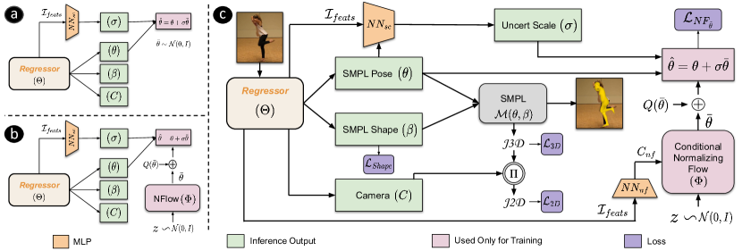
The POCO framework starts with a base HPS regressor and augments the network and training so that the method takes an input image, $I$, and outputs an uncertainty estimate, $\sigma$, in addition to the standard SMPL pose, $\theta$, shape, $\beta$, and weak-perspective camera, $C$, parameters; see Fig. 2 (c).

3.1 Preliminaries

Body model: SMPL [40] is a differentiable parametric human body model. As input, it takes parameters for pose, $\theta\in\mathbb{R}^{72}$, and shape, $\beta\in\mathbb{R}^{10}$. As output, it produces a body mesh, $\mathcal{M}$, and vertices, $V\in\mathbb{R}^{NX3}$, where $N=6890$ is the number of vertices. 3D skeletal joints, $J_{3D}$, are computed from a linear combination of mesh vertices, $V$, using a pre-trained linear regressor $J_{Reg}$, i.e., $J_{3D}=J_{Reg}V$.

Regressor for SMPL bodies: The core idea of POCO can be employed as a component of any regressor network, $\Theta(I)$, that estimates a SMPL body and a camera from an image. Here we evaluate POCO using three different regressors; i.e., HMR [19], PARE [26], and CLIFF [37]. The main difference between these is the way they compute features from the image. HMR uses a ResNet to compute a single global feature from the image; this often causes problems for poses and occlusions that are unseen during training. PARE accounts for this by using human-part-guided attention to compute several per-part features that are aggregated; this gives robustness to occlusions, as the non-occluded parts help resolve ambiguities caused by the occluded ones. HMR and PARE operate on an image cropped around a body. In contrast, CLIFF also considers the body’s location in the full image; this global context helps improve poses. CLIFF represents the current SOTA. For details of each model’s architecture, see Sup. Mat.

Normalizing Flow (NF): These models are used to model arbitrarily complex distributions through a composition of smooth and invertible transformations of a simple distribution. Let $Z\in\mathbb{R}^{d}$ be a random variable from a simple distribution, e.g., a multivariate Gaussian distribution, $P_{Z}(z)$. Let also $f:\mathbb{R}^{d}\rightarrow\mathbb{R}^{d}$ be a smooth and invertible function. The NF transforms $z$ into a complex distribution $x=f(z)$ and, as it is invertible, we can define $z=f^{-1}(x)$. The log probability density function of $x$ is:

$$\textnormal{log}P_{X}(x)=\textnormal{log}P_{Z}(z)+\textnormal{log}\left|\textnormal{det}\frac{\partial f^{-1}}{\partial z}\right|\text{.}$$ (1)

3.2 Unconditional Uncertainty Estimation

Sec. 3.2.1 MSE loss & error distribution: A standard mean-squared-error (MSE) loss, typically used for training HPS models [26, 28], assumes the inferred-sample error to be Gaussian distributed with a constant variance across all samples. Below, we refer to this Gaussian as a base density function (bDF) that is shared among all samples. Kendall et al. [22] replace the constant variance with a per-sample variance, in the context of semantic segmentation.

We adapt the work of Kendall et al. for HPS as shown in  Fig. 2 (a), and use a regressor, $\Theta$, to estimate per-sample parameters for pose, $\theta_{i}$, and variance, $\sigma_{i}$, from an image, $I_{i}$. We define the pose loss over a dataset of $N$ images as:

$$\mathcal{L}_{\theta}=\frac{1}{N}\sum_{i=1}^{N}\frac{1}{2{\sigma}_{i}^{2}}||{\theta_{g}}_{i}-\theta_{i}||^{2}+\frac{1}{2}log({\sigma}_{i}^{2})\text{,}\vspace{-0.5 em}$$ (2)

where ${\sigma}_{i}$ is the predicted per-sample variance from the scale network ($\mathit{NN}_{\mathit{sc}}$), $\theta_{i}$ is the predicted pose, and ${\theta_{g}}_{i}$ is the ground-truth pose. The predicted pose and variance translates and scales the bDF.

To minimize the loss in Eq. 2, the network should infer a large variance, $\sigma$, when the predicted pose is far from the ground-truth one, and small otherwise. To discourage the network from always inferring a large $\sigma$ to naively minimise the loss, the second term of Eq. 2 acts as a regularizer.

Although the above formulation lets networks predict an uncertainty estimate, i.e., the scale $\sigma_{i}$, we show in experiments that this does not correlate well with the pose error. Therefore, we need a more complex and “expressive” bDF.

Sec. 3.2.2 Normalizing Flow (NF): A Normalizing Flow (NF) model [7] represents arbitrarily complex distributions. Thus, we extend the baseline model from above, and replace the Gaussian bDF with a NF network, $f_{\Phi}$; see  Fig. 2 (b). The NF network, $f_{\Phi}$, transforms a simple distribution, $z\backsim\mathcal{N}(0,I)$, to a “deformed” zero-mean distribution $\bar{\theta}\backsim P_{\Phi}(\bar{\theta})$, which is our new bDF. However, as with the Gaussian case, the bDF is the same for all samples. Since the NF is an invertible model, let $\bar{\theta}=f_{\Phi}^{-1}(z)$. We then use a regressor, $\Theta$, to infer pose, $\theta_{i}$, and a per-sample variance, $\sigma_{i}$, that shift and scale the NF distribution $\bar{\theta}$ as:

$$\hat{\theta}=\theta+\bar{\theta}\sigma,\vspace{-0.35 em}$$ (3)

where we drop the image index $i$ for notational simplicity. Using Eq. 1, the NF loss is defined as:

$$\small\begin{split}\mathcal{L_{NF}}&=\left.-\textnormal{log}P_{\Theta,\Phi}(\hat{\theta}|I)\right|_{\hat{\theta}=\theta_{g}}\\ &=-\textnormal{log}P_{\Phi}(\bar{\theta}_{g})-\textnormal{log}\left|\textnormal{det }\frac{\partial f_{\Phi}^{-1}\left(\bar{\theta}_{g}\right)}{\partial\theta_{g}}\right|\\ &=-\textnormal{log}P_{\Phi}(\bar{\theta}_{g})-\textnormal{log}\left|\textnormal{det }\frac{\partial(\theta_{g}-\theta)/\sigma)}{\partial\theta_{g}}\right|\\ &=-\textnormal{log}P_{\Phi}(\bar{\theta}_{g})+\textnormal{log}\sigma\text{,}\end{split}\vspace{-0.35 em}$$ (4)

where $\bar{\theta}_{g}=(\theta_{g}-\theta)/\sigma$ is the scale-normalized error and the subscript $g$ denotes ground truth; note that for formulating the loss we set $\hat{\theta}=\theta_{g}$, which is our goal.

Equation 4 shows that, by using the NF network, $f_{\Phi}$, training entirely depends on the estimation of $f_{\Phi}$; see the term $\textnormal{log}P_{\Phi}(\bar{\theta}_{g})$. We observe (as Li et al. [35]) that this makes convergence challenging in early training stages, when both the regressor and the NF module are untrained.

To tackle this problem, RLE [35] proposes a gradient-shortcut approach. The solution is to introduce another simpler distribution, i.e., a Gaussian $Q(\bar{\theta}_{g})$, which is independent of the NF module. As a result, the regressor network, $\Theta$, directly gets the gradients from the loss defined on $Q(\bar{\theta}_{g})$. The underlying assumption is that $Q(\bar{\theta}_{g})$ roughly matches the inferred-sample error distribution, while the NF models a “residual” that is “added” on top of $Q(\bar{\theta}_{g})$ to eventually model a more complex distribution. Consequently, we modify the loss of Eq. 4, which becomes:

$$\mathcal{L_{NF}}=-\textnormal{log}P_{\Phi}(\bar{\theta}_{g})-\textnormal{log}Q(\bar{\theta}_{g})+\textnormal{log}\sigma\text{.}$$ (5)

3.3 Dual Conditioning Strategy (DCS)

POCO uses a novel Dual Conditioning Strategy to infer uncertainty in a single feed-forward pass by augmenting the bDF and scale network ($\mathit{NN}_{\mathit{sc}}$) with a conditioning vector.

Sec. 3.3.1 Image-conditioned bDF (Cond-bDF): While a Normalizing Flow (NF) can model arbitrarily complex distributions, having a single bDF shared among all samples is a strong assumption. This assumption breaks when training on multiple data sources, as these can have different distributions; a shared bDF struggles to model these. Even though the per-sample inferred pose, $\theta$ and variance, $\sigma$, transform the base density function (Eq. 3), we experimentally show that for complex scenarios like HPS we need to go beyond a single shared bDF. We argue that, by using additional per-sample information, a bDF can represent complex scenarios.

Hence, we use a conditional normalizing flow [64] (Cond-bDF), $f_{\Phi}:\mathbb{R}^{d}\times\mathbb{R}^{c}\rightarrow\mathbb{R}^{d}$, to model the inferred-sample error for HPS, where $d$ is the dimension of the NF input and $c$ is the dimension of the conditioning vector; see Fig. 2 (c). The flow model $f_{\Phi}$ is bijective in $z$ and $\bar{\theta}$, i.e. $z=f_{\Phi}(\bar{\theta};C_{\mathit{nf}})$ and $\bar{\theta}=f_{\Phi}^{-1}(z;C_{\mathit{nf}})$, where $C_{\mathit{nf}}$ is the conditioning vector. The Cond-bDF takes some input vector $C_{\mathit{nf}}$ to model a different bDF, the complexity of which depends on the discriminative power of the conditioning vector. A naive approach would be to use a one-hot encoding of the data source, to denote a different data distribution. However, for a rich dataset, even samples within it could belong to different distributions. Also, using a one-hot encoding as a conditioning vector limits training scalability.

To account for this, we introduce image cues as the conditioning vector. The image features are extracted by the regressor, $\Theta$, and pass through a neural network, $\mathit{NN}_{\mathit{nf}}$, which transforms them into a condition vector, $C_{\mathit{nf}}$. Our proposed conditional NF loss is then:

$$\small\mathcal{L_{NF}}=-\lambda_{\mathit{nf}}\textnormal{log}P_{\Phi}(\bar{\theta}_{g};C_{\mathit{nf}})-\lambda_{q}\textnormal{log}Q(\bar{\theta}_{g})+\lambda_{\sigma}\textnormal{log}\sigma,$$ (6)

where $\lambda_{\mathit{nf}}$, $\lambda_{q}$ and $\lambda_{\sigma}$ are steering weights for each term.

Sec. 3.3.2 Pose-conditioned Scale (Cond-Scale): The scale network, $\mathit{NN}_{\mathit{sc}}$, (Fig. 2 (c)) infers uncertainty as a scale, $\sigma$, that transforms a bDF. All related work conditions $\mathit{NN}_{\mathit{sc}}$ on image features only. Here we argue that it is also important to determine uncertainty based on pose plausibility w.r.t. image evidence. We observe that pose provides a signal that helps $\mathit{NN}_{\mathit{sc}}$ regress uncertainty that is highly correlated with reconstruction quality; this is critical: the pose and the image evidence should be consistent.

In the POCO framework, we infer scale, $\sigma$, and SMPL pose, $\theta$, through different sub-networks. Then, $\mathit{NN}_{\mathit{sc}}$ concatenates pose with down-sampled image features, to create a balanced condition vector with same-dimension components (see Sec. 4 for details). In the ablation experiments, we evaluate the importance of this novel formulation.

Sec. 3.2.3 Overall loss: Given a regressor, we take its loss function and add $\mathcal{L_{NF}}$, as defined above. With the current best practices [18, 26] the overall loss is:

$$\begin{split}\mathcal{L}=\mathcal{L_{NF}}+\lambda_{\beta}\mathcal{L}_{\beta}(\beta,\beta_{g})+&\lambda_{3D}\mathcal{L}_{3D}(J_{3D},J_{3D_{g}})+\\ &\lambda_{2D}\mathcal{L}_{2D}(J_{2D},J_{2D_{g}}),\end{split}\vspace{-0.5 em}$$ (7)

where, $\mathcal{L}_{\beta}$ is a SMPL shape loss, $\mathcal{L}_{J_{3D}}$ is the 3D joint loss and $\mathcal{L}_{J_{2D}}$ is the joint re-projection loss. The 2D joints are calculated using the weak-perspective camera $C$ inferred by the regressor $\Theta$. The ground-truth SMPL shape is denoted by $\beta_{g}$, 3D joints by $J_{3D_{g}}$ and 2D joints by $J_{2D_{g}}$. Finally, $\lambda_{\beta}$, $\lambda_{3D}$ and $\lambda_{2D}$ are steering weights for each term.

4 Implementation details

The POCO framework is applicable to common HPS regressors that infer parametric bodies like SMPL. We show this by using three HPS variants, i.e., HMR-EFT [18] (ResNet-50 [11] backbone), PARE [26] (HRNet-w32 [56] backbone) and CLIFF [37] (HRNet-w48-cls [56] backbone). We call the resulting methods POCO-HMR-EFT, POCO-PARE and POCO-CLIFF, respectively.

Image features, $I_{\mathit{feats}}$, of dimension $2048$, $3072$ and $2048$ are extracted after the global-feature pooling layer in HMR-EFT, the part-attention aggregation layer in PARE, and the classifier layer in CLIFF, respectively. The scale network $\mathit{NN}_{\mathit{sc}}$ is a 2-layer MLP with $\{2048,216\}$ hidden layers. The first layer downsamples image features to a 216D vector before concatenating with the 216D ($24\times 3\times 3$) pose, to get a balanced condition vector. The second layer infers a per-part uncertainty (24D vector); for details and results on per-part uncertainty, see Sup. Mat.

To get a single uncertainty estimate for the full body, we sum the per-part uncertainties along SMPL’s skeleton, normalize to the range of $[0,1]$, and compute the mean. A 1-layer perceptron maps $I_{\mathit{feats}}$ into a 512D conditioning vector $C_{\mathit{nf}}$. Cond-bDF is a 2-block conditional RealNVP [7]; each block has 2 MLP layers of size $\{64,64\}$. For details on the overhead of POCO, see Sup. Mat. We empirically set $\lambda_{\mathit{nf}}=1.0e^{-4}$, $\lambda_{\sigma}=1.0e^{-4}$, $\lambda_{q}=1.0e^{-2}$; other $\lambda$ weights are as in original methods [26, 18, 37]. We train with Adam [23] ($3.0e^{-6}$ learning rate, 64 batch size).

Training: We train POCO-PARE and POCO-HMR-EFT on COCO [39], Human3.6M [15], MPI-INF-3D [42], MPII [1] and LSPET [16]. For datasets without 3D ground truth (GT), we use EFT’s [18] pseudo GT SMPL parameters, and use HMR-EFT’s ratio for mixing 2D and 3D data in a batch. Since CLIFF’s training code is not public, we re-implement it (“CLIFF-Ours”); for details see Sup. Mat. For a fair comparison, we train with CLIFF’s [37] data and mixing ratio. For fast convergence, we start with a pre-trained HPS regressor, and train the full POCO model for 50k iterations. Then, we freeze the backbone and HPS branch and train only the $\mathit{NN}_{\mathit{sc}}$ and Cond-bDF nets for another 10k iterations.

For fair comparisons, for every benchmark setting we use the same training data and schemes as the original HPS models, and use PARE’s data augmentation.

Evaluation & metrics: We evaluate on the test sets of 3DPW [59], 3DOH [75] and 3DPW-OCC [59, 75]. We report three pose metrics ($mm$): the “Procrustes aligned mean per joint position error” (PA-MPJPE), the “mean per joint position error” (MPJPE) and the “per-vertex error” (PVE). We use the “Pearson correlation coefficient” (PCC) as the uncertainty metric to measure the correlation of the estimated uncertainty with pose error.

5 Evaluation

5.1 Performance of POCO Framework

Method	PVE $\downarrow$	MPJPE $\downarrow$	PA-MPJPE $\downarrow$	Type
HMMR [19]	-	116.5	72.6	Dtr
VIBE [25]	113.4	93.5	56.5	Dtr
Pose2Mesh [6]	-	89.2	58.9	Dtr
Zanfir et al. [6]	-	90.0	57.1	Dtr
I2L-MeshNet [44]	-	93.2	58.6	Dtr
HMR [19]	-	130.0	76.7	Dtr
SPIN [28]	135.1	96.9	59.2	Dtr
DSR [8]	105.8	91.7	54.1	Dtr
HybriK [36]†	86.5	74.1	45.0	Dtr
Biggs et al. [3]	-	93.8	59.9	Prob
ProHMR [30]	-	-	55.1	Prob
Sengupta et al. [51]	-	84.9	53.6	Prob
HuManiFlow [52]	-	83.9	53.4	Prob
HMR-EFT [18]	106.1	92.5	54.2	Dtr
POCO-HMR-EFT	101.1	88.5	52.4	Prob
POCO-HMR-EFT-pGT	99.7	87.3	51.5	Prob
PARE [26]	97.9	82.0	50.9	Dtr
POCO-PARE	95.3	80.3	49.9	Prob
POCO-PARE-pGT	94.0	79.5	49.4	Prob
CLIFF-Ours [37]†	85.8	72.8	44.5	Dtr
POCO-CLIFF-Ours †	84.6	70.9	43.3	Prob
POCO-CLIFF-Ours-pGT†	83.5	69.7	42.8	Prob

Table 1: Evaluation of POCO & SOTA HPS on 3DPW (Sec. 5.1). All metrics are in mm. CLIFF-Ours is our re-implementation of CLIFF [37], and ^† denotes that 3DPW is used for training. Suffix “-pGT” denotes self-improved training for several POCO variants (see Sec. 5.4, task 1). “Dtr” and “Prob” refers to deterministic and probabilistic methods, respectively.

	3DPW-OCC [75, 59]			3DOH [75]
Method	PVE $\downarrow$	MPJPE $\downarrow$	PA-MPJPE $\downarrow$	MPJPE $\downarrow$	PA-MPJPE $\downarrow$
Zhang et al. [75]	-	-	72.2	-	58.5
SPIN [28]	121.6	95.6	60.8	104.3	68.3
PARE [26]	111.3	90.5	56.6	63.3	44.3
POCO-PARE	109.1	89.0	54.5	61.0	42.5

Table 2: Evaluation on occlusion datasets (Sec. 5.1). All metrics are in mm. All methods use a ResNet-50 baseline.

We compare recent HPS models and POCO-HPS (building on three recent HPS models: HMR-EFT, PARE, CLIFF) on 3DPW’s test set in Tab. 1 We list two method types: (1) “deterministic” ones (Dtr), inferring SMPL parameters, and (2) “probabilistic” ones, inferring a distribution either over SMPL parameters or sample error in case of POCO-HPS. The most direct comparison is with HMR-EFT, PARE and CLIFF that use the same architecture and training; POCO-HPS outperforms its base HPS model. Note that some probabilistic methods (i.e., ProHMR) infer multiple bodies, but POCO infers only one.

We also evaluate on occlusion datasets (3DPW-OCC [75, 59] and 3DOH [75]) in Tab. 2. We train POCO-PARE with a ResNet-50 baseline as all other models. All models but SPIN train on COCO, Human3.6M and 3DOH. POCO-PARE performs best; our framework helps improve HPS.

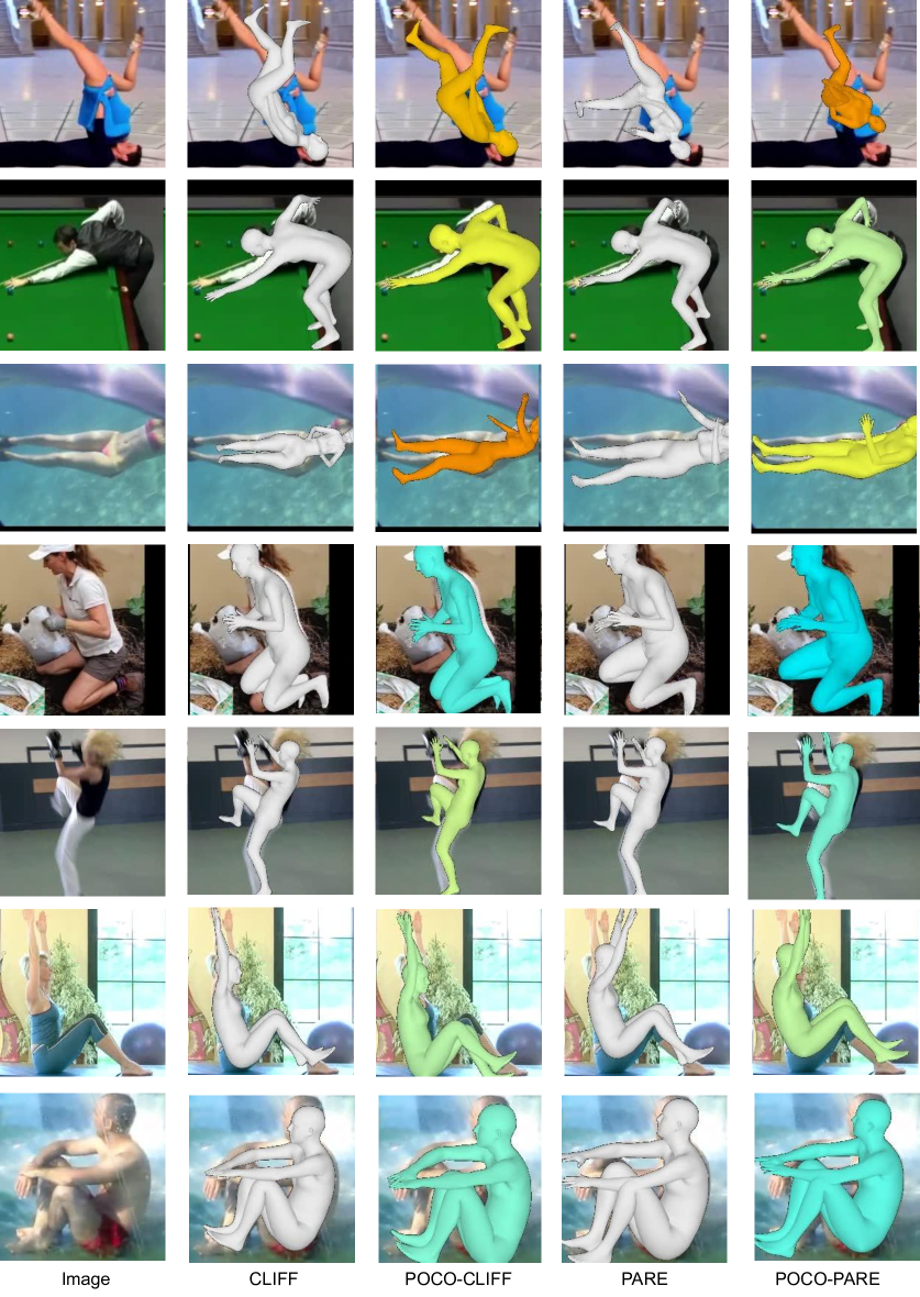
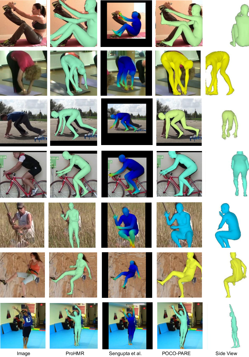
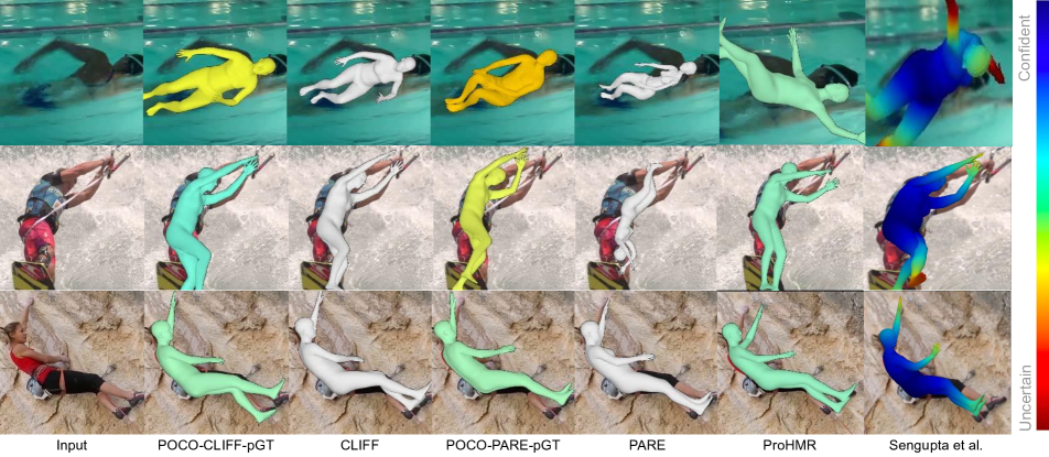
We qualitatively compare POCO-HPS with its “deterministic” HPS model (PARE [26], CLIFF [37]) and “probabilistic” HPS models (Sengupta et al. [51], ProHMR [30]) in Fig. 3. The former do not represent uncertainty (bodies shown in gray color), while for the latter, uncertainty is visualized color-coded (see bar in Fig. 3). Sengupta et al. sample 64 SMPL bodies and compute uncertainty as the per-vertex variance. For ProHMR we do the same sampling, but compute SMPL-pose variance and take the mean along SMPL’s skeleton as uncertainty, like POCO does (see Sec. 4). POCO-HPS outperforms its base HPS model in challenging cases. ProHMR infers similar uncertainty values across images (see consistent “aquamarine” color), irrespective of image ambiguities or the inferred pose quality. Sengupta et al. consistently infer high uncertainty for end-effectors in a narrow range, having an inductive bias. POCO-HPS infers better SMPL bodies, and an uncertainty that is better correlated with its output quality.

5.2 Performance of Uncertainty Formulations

We compare the performance of our uncertainty formulation (i.e., our Dual Conditioning Strategy) with existing uncertainty formulations [22, 35] on 3DPW [59]; see Tab. 3. We use HMR-EFT [18] as the HPS model to evaluate the performance of each formulation; for other HPS models see Sup. Mat. All models are trained on the same data.

We adapt the uncertainty formulation of Kendall et al. [22] (Gauss) and RLE [35] (NFlow) for HPS (2nd and 3rd row, respectively, in Tab. 3). Following their approach, we use a Gaussian distribution in Gauss and use normalizing flow (NF) in NFlow. The pose metrics slightly improve when the network is forced to estimate uncertainty. However, with POCO’s uncertainty formulation (5th row in Tab. 3), the pose metrics and the uncertainty metric (PCC) improve significantly compared to prior methods; depicting the efficacy of our framework. The PCC metric shows how uncertainty correlates with pose error; a higher value denotes a stronger correlation.

5.3 Performance of POCO Components

POCO introduces a novel Dual Conditioning Strategy which consists of Cond-bDF (Sec. 3.3.1) and Cond-Scale (Sec. 3.3.2). We evaluate the performance of each component; see 4th and 5th row of Tab. 3. For Cond-Scale, we use NF as bDF and condition scale inference (via $\mathit{NN}_{\mathit{sc}}$) on pose, and get further improvement. For Cond-bDF, we realize that images can look very different, even within the same dataset, and cannot all share the same bDF. Intuitively, images that lie close-by in a feature space can share a bDF, distant ones can not. We add image features as (via $\mathit{NN}_{\mathit{nf}}$) for the NF network; this also boosts performance.

The Dual Conditioning Strategy of our POCO framework (6th row of Tab. 3) results in the best performance for all metrics, showing that the above two design choices contribute positively and are complementary. Comparing POCO with pure-HPS models (first row of Tab. 3) shows a notable difference. Perhaps surprisingly, as this was not our goal, pushing our model to solve a harder task, i.e., perform both HPS and uncertainty inference, improves HPS performance; this aligns with findings in multi-task learning [71].

POCO Variants	PVE $\downarrow$	MPJPE $\downarrow$	PA-MPJPE $\downarrow$	PCC $\uparrow$
HMR-EFT [18]	106.1	92.5	54.2	-
+ Gauss [22]	105.7	92.3	54.1	0.31
+ NFlow [35]	104.9	91.2	53.7	0.42
+ Cond-Scale	103.5	89.9	53.3	0.44
+ Cond-bDF	103.2	89.8	53.1	0.46
+ POCO	101.1	88.5	52.4	0.52
POCO-HMR-EFT-pGT	99.7	87.3	51.5	0.53

Table 3: Evaluation of POCO (Sec. 5.3) and other uncertainty methods on 3DPW (Sec. 5.2). PCC is in the range $\in[-1,1]$. We evaluate on 3DPW’s test set [59]; no model was trained on 3DPW. Suffix “-pGT” denotes self-improved training (Sec. 5.4, task 1). The row “+POCO” denotes the model “POCO-HMR-EFT”.

Figure 3: Qualitative results for in-the-wild images. We evaluate CLIFF-Ours [37], PARE [26], ProHMR [30], Sengupta et al. [51] and our POCO built on two different HPS regressors. For more results see Sup. Mat.

Figure 4: Infilling with uncertainty. Given estimated 3D bodies for detected people in a video, GLAMR [70] infills 3D bodies for missing detections, and does sequence-level refinement for these. (a) However, GLAMR considers all estimated 3D bodies as accurate, and fails when they are not. (b) POCO provides both 3D bodies and an uncertainty metric; this helps GLAMR reject uncertain bodies and infill also for these. See middle frame for a/b. For video results, see the video on our website.

5.4 Downstream Tasks

We show the usefulness of POCO’s uncertainty for two downstream applications, as discussed in the following.

Task 1: Self-improved: HPS Training To train robust HPS regressors, we need highly-varied images paired with high-quality 3D bodies. Datasets with 3D ground truth (GT) are small and captured in lab settings, thus, recovering good pseudo-GT [18] from in-the-wild images has proven to be helpful. However, this typically requires human annotators to manually curate good HPS reconstructions [18].

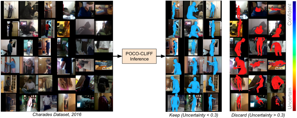
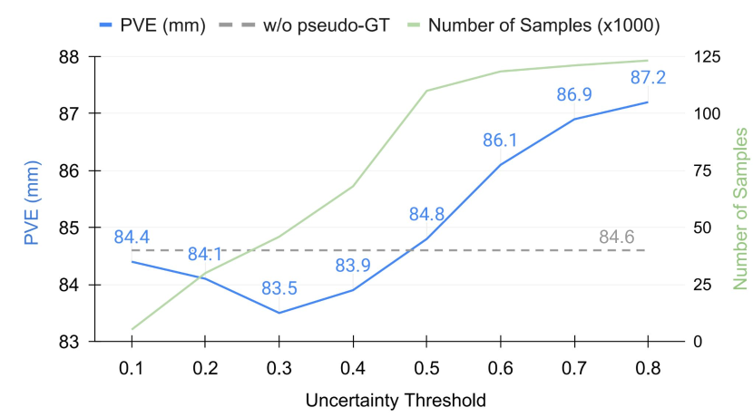
We automate this with POCO. We use the model’s uncertainty measure to recover 3D bodies from Charades [54], a dataset with in-the-wild videos of daily activities. By using POCO’s uncertainty, which is correlated with its output quality, we automatically curate the SMPL estimates with low uncertainty; we use a strict uncertainty threshold of $0.3$ and keep only estimates below it; for details see Sup. Mat. We treat the curated bodies as pseudo-GT, add this to the existing training data, and fine-tune POCO variants; these self-improved models are denoted with the “-pGT” suffix.

We evaluate the self-improved models on 3DPW; see bottom of Tabs. 1 and 3, “-pGT” entries. Unsurprisingly, they improve all error metrics (PVE, MPJPE). In Tab. 3 the self-improved model has the same correlation (PCC) between uncertainty and output quality. We hypothesize that pseudo-GT contributes highly-varied images that improve HPS, but the strict uncertainty threshold contributes less-varied uncertainty labels. We also vary the uncertainty threshold and observe that for higher thresholds, the performance decreases, showing that higher uncertainty corresponds to low quality pseudo-GT; for details see Sup. Mat.

Task 2: 4D bodies from videos To recover 4D bodies from videos, methods like GLAMR [70] infer per-frame SMPL bodies via an HPS model, and post-process them to improve temporal quality, while “infilling” frames with missing detections. However, existing methods cannot automatically curate the “good” SMPL estimates, consequently, results may be “contaminated” with HPS failures.

We address this with POCO. First, we run POCO on a sequence and estimate per-frame bodies along with uncertainty. We use a threshold of $0.8$, discard estimates with uncertainty values above this, and consider these rejected frames as “missing”. We then use GLAMR’s infiller to generate the missing bodies and perform global optimization for refinement. By rejecting the uncertain bodies, the infiller has to work harder but relies on neighboring high-quality poses. As seen in Fig. 4, POCO helps recover accurate HPS sequences for videos using its uncertainty measure. In such scenarios, standard HPS models have a clear disadvantage. The above shows that POCO’s HPS performance and uncertainty inference are promising and useful.

6 Conclusion

While a huge progress has been made in estimating 3D human bodies from an image, most regressors do not have a measure for the output’s quality. Thus, downstream applications do not know how much to rely on them, and struggle with bad outputs. We account for this with POCO, a novel framework that infers SMPL bodies along with its uncertainty. Experiments show that POCO’s uncertainty is correlated with the quality of pose reconstruction. We also show that POCO can build on three different HPS models; this is promising for also using future ones. Finally, we show the usefulness of uncertainty for practical applications.

Future work: POCO models pose uncertainty; this can be extended also for shape; for discussion see Sup. Mat. For reconstructing challenging videos in 4D, methods like GLAMR [70] can benefit from POCO’s uncertainty estimate. We think that POCO will probe further work on uncertainty for HPS.

Acknowledgements: We sincerely thank Partha Ghosh and Haiwen Feng for insightful discussions and Priyanka Patel for CLIFF reference implementation. We also thank Peter Kulits, Shashank Tripathi, Muhammed Kocabas and rest of Perceiving Systems department for their feedback. The authors thank the International Max Planck Research School for Intelligent Systems (IMPRS-IS) for supporting Sai Kumar Dwivedi. This work was partially supported by the German Federal Ministry of Education and Research (BMBF): Tübingen AI Center, FKZ: 01IS18039B.

MJB has received research gift funds from Adobe, Intel, Nvidia, Meta/Facebook, and Amazon. MJB has financial interests in Amazon, Datagen Technologies, and Meshcapade GmbH. While MJB is a part-time employee of Meshcapade, his research was performed solely at, and funded solely by, the Max Planck Society.

POCO: 3D Pose and Shape Estimation with Confidence
**Supplementary Material**

In this Supplementary-Material document, we provide more details about our method. Additionally, please see the video on our website for a summary of the method and more visualizations of the results.

Appendix A Regressor Network Architecture

We use three variants of HPS regressors in POCO, i.e., PARE [26], HMR-EFT [18], CLIFF [37] as shown in  Fig. S.1.

In PARE, the input image is first passed through a CNN backbone (HRNet-32W), and features are extracted before the average pooling layer. The features are then passed through two separate branches: a 2D Part Segmentation branch and a 3D Body Feature branch. The 2D part segmentation branch produces body-part attention features $S\in\mathbb{R}^{H\times W\times(J+1)}$, where $J=24$ is the number of SMPL body parts, while a background mask is assigned to non-human pixels. The body feature branch is used to estimate SMPL body parameters. Both branches produce features of the same spatial dimensions, $H\times W$. The features from $S$ pass through a spatial softmax normalization layer, $\kappa$. These are used as soft attention masks to aggregate 3D body features into final features, $F=\kappa(S)^{\top}\odot B$, where $S\in\mathbb{R}^{HW\times J}$, $B\in\mathbb{R}^{HW\times C}$ and $F\in\mathbb{R}^{J\times C}$; note that $S$ and $B$ are reshaped before the operation. Each feature row, $F_{i}\in\mathbb{R}^{1\times C}$ with $i\in\{1,\dots,J\}$, passes through a separate MLP to get SMPL pose parameters, $\theta=\{\theta_{i}\}$. To estimate the camera, $C$, and SMPL shape, $\beta$, all final features $F$ are fed, concatenated, to different MLPs.

Figure S.1: Regressor architecture.

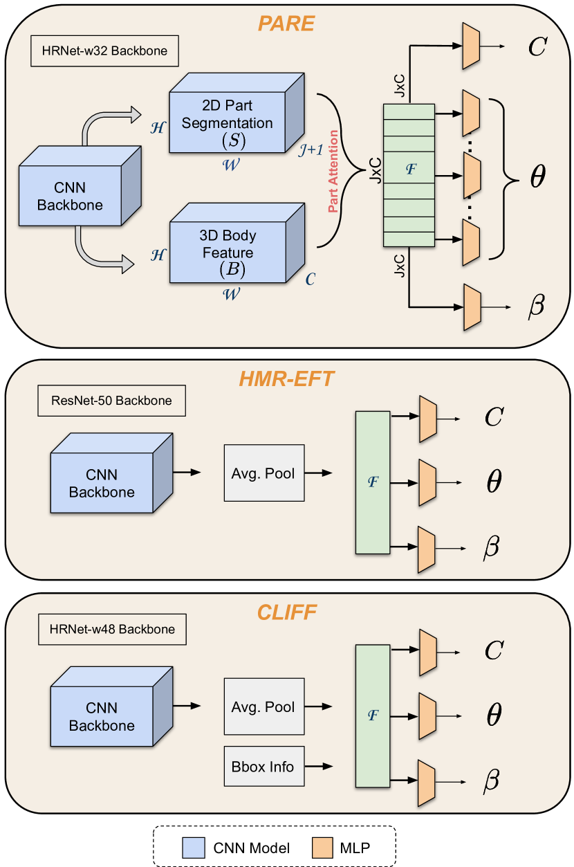
HMR-EFT uses a simple network architecture for estimating HPS. The input image passes through a CNN backbone (ResNet-50) followed by a global average pooling layer. The features from the pooling layer are used to regress SMPL pose, $\theta$, shape, $\beta$, and camera parameters, $C$, through separate MLPs. This regression is done through an iterative error feedback loop.

CLIFF uses a HRNet-w48 network architecture as a CNN backbone. Along with the a cropped image, CLIFF takes the bounding box location information (Bbox Info) as input to provide the location information of the person in the image. This helps to accurately predict the global rotation in the original camera coordinate frame. The bounding box formation contains the center of bounding box center relative to image center and focal length of the original camera which is calculated using image height and width. Contrary to PARE and HMR-EFT, CLIFF computes a 2D keypoint loss after projecting the body keypoints onto the original image plane.

Appendix B CLIFF Training and Evaluation

Since the CLIFF training code is not public, we re-implement it (“CLIFF-Ours”). We train CLIFF-Ours on COCO [39], MPII [1], MPI-INF-3D [42], H3.6M [15] and 3DPW [59] with the same dataset ratios used in HMR-EFT [18]. For 2D datasets, we use the pseudo ground-truth SMPL parameters provided by CLIFF and, for other datasets, we use the the original annotations provided by the respective datasets. Following prior work [26, 18], we resize the cropped image to $224\times 224$ for both training and evaluation. To compute the 2D keypoint loss on full image plane, first we crop the keypoints according to the person bounding box and then project them back to the original image size. To evaluate on 3DPW test, we use the same bounding box scale and center used by prior work [26, 28].

Method	HMR-EFT [17]		PARE [26]		CLIFF [37]
	PVE $\downarrow$	PCC $\uparrow$	PVE $\downarrow$	PCC $\uparrow$	PVE $\downarrow$	PCC $\uparrow$
Baseline HPS	106.1	-	97.9	-	85.8	-
Gauss [22]	105.7	0.31	97.1	0.32	85.4	0.29
NFlow [35]	104.9	0.42	96.6	0.44	85.3	0.40
POCO-HPS	101.1	0.52	95.3	0.54	84.6	0.51

Table S.1: Evaluation of POCO and other uncertainty formulations for different HPS regressors.

Appendix C Performance of Uncertainty Formulations for different HPS regressors

We compare the performance of our uncertainty formulation (i.e., our Dual Conditioning Strategy) with existing uncertainty formulations [22, 35] on 3DPW [59] for different HPS regressors [19, 26, 37] as shown in Tab. S.1. This complements Tab. 3 in the main paper. Our uncertainty formulation outperforms the prior formulations (Gauss and NFlow) for all HPS regressors in both the pose (PVE) and uncertainty (PCC) metrics. Note that the PCC metric should not be compared across different HPS methods on its own. Focusing separately on each HPS method, the important thing is that our novel uncertainty formulation consistently lowers PVE errors while increasing the PCC metric; this is indicative of a better uncertainty formulation.

Appendix D Per-Part and Per-Vertex Uncertainty

Figure S.2: Per-part uncertainty of POCO-CLIFF. For each image triplet: input image, per-part uncertainty of POCO and whole-body uncertainty of POCO.

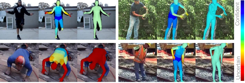
POCO models the uncertainty of SMPL pose parameters in the following way. First, it estimates the uncertainty for the axis-angle rotation of each of SMPL’s skeleton joints separately. This is important because each of these has a different amount of error. However, for downstream applications, having a single uncertainty value for the full body is more practical. To this end, we traverse SMPL’s kinematic chain (i.e., recursively going in the direction from parent to child), and add the axis-angle uncertainties of the respective skeleton joints; as there 24 joints in total, this produces a 24D vector. We then normalize the 24D vector to the range of $[0,1]$ and compute the mean to get a single scalar uncertainty value; this represents the uncertainty for the full body. The per-part uncertainties and the full-body uncertainty are shown in  Fig. S.2.

A few recent methods [51, 52] show per-vertex uncertainties. They do so by sampling multiple bodies and computing uncertainty as per-vertex variance. While this is an interesting choice, modelling per-vertex uncertainties in a single feed-forward pass would be expensive. One would need to model the base density function and scale network to output $6890$ (SMPL vertices) as compared to only $24$ variables (SMPL joints) in the case of POCO.

Appendix E Overhead of POCO Framework

Method	Train-Params	Test-Params	Inference Time
CLIFF	81.0 M	81.0 M	1.45 ms
POCO-CLIFF	82.6 M	81.3 M	1.49 ms

Table S.2: POCO’s overhead when applied to HPS regressor.

POCO is a general uncertainty framework that can be applied to common HPS methods, extending them to also estimate uncertainty. It adds a bDF and scale network for estimating uncertainty in a single network pass. Tab. S.2 shows that POCO imposes only a small overhead. POCO-CLIFF has only 2% more training parameters than CLIFF due to adding the bDF and scale network. The former is unused at test time and the latter is just a small NN, so, adding POCO increases inference time only minimally.

Figure S.3: Uncertainty threshold for pseudo-GT selection. Using an optimal uncertainty threshold of $0.3$ for selecting pseudo-GT from Charades dataset [54] for training, POCO-CLIFF-pGT’s performance on 3DPW test set is better than the model trained without it (dashed line). The performance degrades with higher uncertainty threshold. PVE denotes per-vertex error. The green line is for number of samples and axis is on the right.

Appendix F Self-Improved HPS Training

POCO estimates an uncertainty measure that correlates with pose reconstruction quality. We use this measure to automatically curate SMPL estimates from the Charades dataset [54] and improve POCO, using the following steps.

We first sample every 100th frame from the videos to get a total of $130$K images, and apply POCO on these. We then vary POCO’s uncertainty threshold, and for each value we automatically curate the produced SMPL estimates and extend POCO’s training data. This results in multiple extended training datasets. We finetune POCO separately for each of these, and evaluate each finetuned model on 3DPW.

The evaluation results are shown in Fig. S.3. The dashed gray line shows the original POCO (with no additional pseudo-GT). The blue curve shows the PVE error (mm) of the finetuned variants. The green curve shows the number of curated samples for each threshold. With a low threshold ($0.1$) very few samples pass, thus, performance is almost unchanged. With a high threshold ($\geq 0.45$), as the threshold gets higher, more samples of decreasing quality pass, which can even harm performance. For thresholds in the range of $\bigl{[}0.2,0.4\bigr{]}$ enough good-quality samples pass so that performance improves. The best performance is achieved for a threshold of $0.3$, which results in adding roughly 46k samples in the training dataset; given the limited number of subjects and pose variation compared to the original dataset, the performance shows that this bootstrapping is promising. Note that the threshold is determined on the Charades dataset by visual inspection. 3DPW test data is not used in setting the threshold. Random samples of pseudo ground-truth generated by POCO-CLIFF on Charades dataset is shown in  Fig. S.5.

Method	PVE $\downarrow$	MPJPE $\downarrow$	PA-MPJPE $\downarrow$	Filter pGT	# pGT
POCO-CLIFF	84.6	70.9	43.3	-	-
POCO-CLIFF-Whole	87.2	74.7	46.1	✗	130K
POCO-CLIFF-Rand	86.6	73.9	45.6	✗	46K
POCO-CLIFF-pGT	83.5	69.7	42.8	✓	46K

Table S.3: Effect of uncertainty-filtered pGT data on 3DPW. “Whole” trains with all data [54] without filtering, “Rand” with random samples, and “pGT” filters using POCO uncertainty.

To better understand the value of self-improvement, we perform two additional baseline experiments. POCO-CLIFF-pGT uses 46K frames (out of 130K) from the Charades dataset, filtered using our uncertainty estimates. For comparison, we re-train POCO-CLIFF: (1) using all 130K frames (“Whole”), and (2) using 46K frames randomly sampled from the 130K (“Rand”). All methods use POCO-CLIFF SMPL estimates as pGT. Tab. S.3 shows that adding data without confidence filtering makes results worse, while our self-improvement process improves them.

Figure S.4: Failure cases of POCO. In some cases of occlusion and out-of-distribution poses, POCO estimates high uncertainty even though the pose reconstructions are not totally implausible.

Appendix G Failure Cases

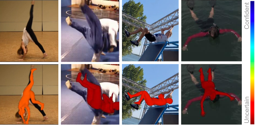
In Fig. Fig. S.4, we show some representative cases in which POCO’s prediction quality and its uncertainty estimate disagree. Typically, POCO produces more plausible poses than other HPS methods [26, 10], even for complex scenarios of heavy occlusion and out-of-distribution poses. However, sometimes POCO estimates high uncertainty, even if the poses it produces are reasonable; think of this a “false negative”. In Fig. S.4 each image either contains an unusual pose, motion blur, occlusion, or dim lighting – in some cases more than one of these. It is reasonable for the network to be uncertain of its estimates in these cases, even if it happens to get the pose right (or close).

Appendix H Effect of Occlusion on Uncertainty

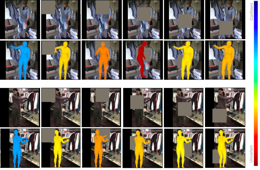
POCO estimates 3D body parameters and their uncertainty in a single feed-forward pass. The uncertainty is correlated to image ambiguities and the quality of reconstruction. We analyze the correlation qualitatively on 3DPW for the POCO-HMR-EFT network. Specifically, we add a synthetic occluder that we swipe throughout the video frames to see the effect on uncertainty; see Fig. S.6. We observe that uncertainty increases when a body part is occluded.

Appendix I Qualitative Results

Figure S.5: Automatic pseudo-GT. Random samples of pseudo-GT generated by POCO-CLIFF on Charades [54] dataset. We keep the frames with lower uncertainty and treat the output SMPL parameters as pseudo ground-truth for re-training.

Figure S.6: Effect of occlusion on uncertainty. When an image becomes ambiguous due to a synthetic occluder, POCO-HMR-EFT estimates a higher uncertainty.

Figure S.7: Qualitative evaluation for in-the-wild images. We show results for CLIFF [37], PARE [26] and POCO versions of respective HPS methods i.e. POCO-CLIFF and POCO-PARE.

Figure S.8: Qualitative evaluation for in-the-wild images. We show results for ProHMR [30], Sengupta et al. [10], and our POCO-PARE.

We qualitatively compare POCO with the deterministic HPS methods like CLIFF [37], PARE [26], and the probabilistic methods ProHMR [30] and Sengupta et al. [10]. The results are shown in  Fig. S.7 and  Fig. S.8, respectively. For more qualitative examples, please see the video on our website.

References

- Andriluka et al. [2014] Mykhaylo Andriluka, Leonid Pishchulin, Peter Gehler, and Bernt Schiele. 2d human pose estimation: New benchmark and state of the art analysis. In Computer Vision and Pattern Recognition (CVPR), 2014.
- Anguelov et al. [2005] Dragomir Anguelov, Praveen Srinivasan, Daphne Koller, Sebastian Thrun, Jim Rodgers, and James Davis. SCAPE: Shape completion and animation of people. Transactions on Graphics (TOG), 2005.
- Biggs et al. [2020] Benjamin Biggs, David Novotny, Sebastien Ehrhardt, Hanbyul Joo, Ben Graham, and Andrea Vedaldi. 3D multi-bodies: Fitting sets of plausible 3D human models to ambiguous image data. In Conference on Neural Information Processing Systems (NeurIPS), 2020.
- Blundell et al. [2015] Charles Blundell, Julien Cornebise, Koray Kavukcuoglu, and Daan Wierstra. Weight uncertainty in neural networks. In International Conference on Machine Learning (ICML), 2015.
- Bogo et al. [2016] Federica Bogo, Angjoo Kanazawa, Christoph Lassner, Peter Gehler, Javier Romero, and Michael J. Black. Keep it SMPL: Automatic estimation of 3D human pose and shape from a single image. In European Conference on Computer Vision (ECCV), 2016.
- Choi et al. [2020] Hongsuk Choi, Gyeongsik Moon, and Kyoung Mu Lee. Pose2Mesh: Graph convolutional network for 3D human pose and mesh recovery from a 2D human pose. In European Conference on Computer Vision (ECCV), 2020.
- Dinh et al. [2017] Laurent Dinh, Jascha Sohl-Dickstein, and Samy Bengio. Density estimation using real NVP. In International Conference on Learning Representations (ICLR), 2017.
- Dwivedi et al. [2021] Sai Kumar Dwivedi, Nikos Athanasiou, Muhammed Kocabas, and Michael J. Black. Learning to regress bodies from images using differentiable semantic rendering. In International Conference on Computer Vision (ICCV), 2021.
- Gal and Ghahramani [2016] Yarin Gal and Zoubin Ghahramani. Dropout as a bayesian approximation: Representing model uncertainty in deep learning. In International Conference on Machine Learning (ICML), 2016.
- Georgakis et al. [2020] Georgios Georgakis, Ren Li, Srikrishna Karanam, Terrence Chen, Jana Košecká, and Ziyan Wu. Hierarchical kinematic human mesh recovery. In European Conference on Computer Vision (ECCV), 2020.
- He et al. [2016] Kaiming He, Xiangyu Zhang, Shaoqing Ren, and Jian Sun. Deep residual learning for image recognition. In Computer Vision and Pattern Recognition (CVPR), 2016.
- Hornauer and Belagiannis [2022] Julia Hornauer and Vasileios Belagiannis. Gradient-based uncertainty for monocular depth estimation. In European Conference on Computer Vision (ECCV), 2022.
- Huang et al. [2017a] Gao Huang, Yixuan Li, Geoff Pleiss, Zhuang Liu, John E Hopcroft, and Kilian Q. Weinberger. Snapshot ensembles: Train 1, get m for free. In International Conference on Learning Representations (ICLR), 2017a.
- Huang et al. [2017b] Yinghao Huang, Federica Bogo, Christoph Lassner, Angjoo Kanazawa, Peter V Gehler, Javier Romero, Ijaz Akhter, and Michael J. Black. Towards accurate marker-less human shape and pose estimation over time. In International Conference on 3D Vision (3DV), 2017b.
- Ionescu et al. [2014] Catalin Ionescu, Dragos Papava, Vlad Olaru, and Cristian Sminchisescu. Human3.6M: Large scale datasets and predictive methods for 3D human sensing in natural environments. Transactions on Pattern Analysis and Machine Intelligence (TPAMI), 2014.
- Johnson and Everingham [2011] Sam Johnson and Mark Everingham. Learning effective human pose estimation from inaccurate annotation. In Computer Vision and Pattern Recognition (CVPR), 2011.
- Joo et al. [2018] Hanbyul Joo, Tomas Simon, and Yaser Sheikh. Total capture: A 3D deformation model for tracking faces, hands, and bodies. In Computer Vision and Pattern Recognition (CVPR), 2018.
- Joo et al. [2020] Hanbyul Joo, Natalia Neverova, and Andrea Vedaldi. Exemplar fine-tuning for 3D human pose fitting towards in-the-wild 3D human pose estimation. In International Conference on 3D Vision (3DV), 2020.
- Kanazawa et al. [2018] Angjoo Kanazawa, Michael J. Black, David W. Jacobs, and Jitendra Malik. End-to-end recovery of human shape and pose. In Computer Vision and Pattern Recognition (CVPR), 2018.
- Kanazawa et al. [2019] Angjoo Kanazawa, Jason Y. Zhang, Panna Felsen, and Jitendra Malik. Learning 3D human dynamics from video. In Computer Vision and Pattern Recognition (CVPR), 2019.
- Kawashima et al. [2021] Takumi Kawashima, Qina Yu, Akari Asai, Daiki Ikami, and Kiyoharu Aizawa. The aleatoric uncertainty estimation using a separate formulation with virtual residuals. In International Conference on Pattern Recognition (ICPR), 2021.
- Kendall and Gal [2017] Alex Kendall and Yarin Gal. What uncertainties do we need in bayesian deep learning for computer vision? In Conference on Neural Information Processing Systems (NeurIPS), 2017.
- Kingma and Ba [2014] Diederik P. Kingma and Jimmy Ba. Adam: A method for stochastic optimization. In International Conference on Learning Representations (ICLR), 2014.
- Klodt and Vedaldi [2018] Maria Klodt and Andrea Vedaldi. Supervising the new with the old: Learning SFM from SFM. In European Conference on Computer Vision (ECCV), 2018.
- Kocabas et al. [2020] Muhammed Kocabas, Nikos Athanasiou, and Michael J. Black. VIBE: Video inference for human body pose and shape estimation. In Computer Vision and Pattern Recognition (CVPR), 2020.
- Kocabas et al. [2021a] Muhammed Kocabas, Chun-Hao P. Huang, Otmar Hilliges, and Michael J. Black. PARE: Part attention regressor for 3D human body estimation. In International Conference on Computer Vision (ICCV), 2021a.
- Kocabas et al. [2021b] Muhammed Kocabas, Chun-Hao P. Huang, Joachim Tesch, Lea Müller, Otmar Hilliges, and Michael J. Black. SPEC: Seeing people in the wild with an estimated camera. In International Conference on Computer Vision (ICCV), 2021b.
- Kolotouros et al. [2019a] Nikos Kolotouros, Georgios Pavlakos, Michael J. Black, and Kostas Daniilidis. Learning to reconstruct 3D human pose and shape via model-fitting in the loop. In International Conference on Computer Vision (ICCV), 2019a.
- Kolotouros et al. [2019b] Nikos Kolotouros, Georgios Pavlakos, and Kostas Daniilidis. Convolutional mesh regression for single-image human shape reconstruction. In Computer Vision and Pattern Recognition (CVPR), 2019b.
- Kolotouros et al. [2021] Nikos Kolotouros, Georgios Pavlakos, Dinesh Jayaraman, and Kostas Daniilidis. Probabilistic modeling for human mesh recovery. In International Conference on Computer Vision (ICCV), 2021.
- Kundu et al. [2022] Jogendra Nath Kundu, Siddharth Seth, Pradyumna YM, Varun Jampani, Anirban Chakraborty, and R Venkatesh Babu. Uncertainty-aware adaptation for self-supervised 3D human pose estimation. In Computer Vision and Pattern Recognition (CVPR), 2022.
- Lakshminarayanan et al. [2017] Balaji Lakshminarayanan, Alexander Pritzel, and Charles Blundell. Simple and scalable predictive uncertainty estimation using deep ensembles. In Conference on Neural Information Processing Systems (NeurIPS), 2017.
- Lassner et al. [2017] Christoph Lassner, Javier Romero, Martin Kiefel, Federica Bogo, Michael J. Black, and Peter Gehler. Unite the people: Closing the loop between 3D and 2D human representations. In Computer Vision and Pattern Recognition (CVPR), 2017.
- Li and Lee [2019] Chen Li and Gim Hee Lee. Generating multiple hypotheses for 3D human pose estimation with mixture density network. In Computer Vision and Pattern Recognition (CVPR), 2019.
- Li et al. [2021a] Jiefeng Li, Siyuan Bian, Ailing Zeng, Can Wang, Bo Pang, Wentao Liu, and Cewu Lu. Human pose regression with residual log-likelihood estimation. In International Conference on Computer Vision (ICCV), 2021a.
- Li et al. [2021b] Jiefeng Li, Chao Xu, Zhicun Chen, Siyuan Bian, Lixin Yang, and Cewu Lu. HybrIK: A hybrid analytical-neural inverse kinematics solution for 3D human pose and shape estimation. In Computer Vision and Pattern Recognition (CVPR), 2021b.
- Li et al. [2022] Zhihao Li, Jianzhuang Liu, Zhensong Zhang, Songcen Xu, and Youliang Yan. CLIFF: Carrying location information in full frames into human pose and shape estimation. In European Conference on Computer Vision (ECCV), 2022.
- Lin et al. [2021] Kevin Lin, Lijuan Wang, and Zicheng Liu. Mesh graphormer. In International Conference on Computer Vision (ICCV), 2021.
- Lin et al. [2014] Tsung-Yi Lin, Michael Maire, Serge J. Belongie, James Hays, Pietro Perona, Deva Ramanan, Piotr Dollár, and C. Lawrence Zitnick. Microsoft coco: Common objects in context. In European Conference on Computer Vision (ECCV), 2014.
- Loper et al. [2015] Matthew Loper, Naureen Mahmood, Javier Romero, Gerard Pons-Moll, and Michael J. Black. SMPL: A skinned multi-person linear model. In Transactions on Graphics (TOG), 2015.
- Louizos and Welling [2017] Christos Louizos and Max Welling. Multiplicative normalizing flows for variational bayesian neural networks. In International Conference on Machine Learning (ICML), 2017.
- Mehta et al. [2017] Dushyant Mehta, Helge Rhodin, Dan Casas, Pascal V. Fua, Oleksandr Sotnychenko, Weipeng Xu, and Christian Theobalt. Monocular 3d human pose estimation in the wild using improved cnn supervision. In International Conference on 3D Vision (3DV), 2017.
- Mihajlovic et al. [2022] Marko Mihajlovic, Shunsuke Saito, Aayush Bansal, Michael Zollhoefer, and Siyu Tang. COAP: Compositional articulated occupancy of people. In Computer Vision and Pattern Recognition (CVPR), 2022.
- Moon and Lee [2020] Gyeongsik Moon and Kyoung Mu Lee. I2L-MeshNet: Image-to-lixel prediction network for accurate 3D human pose and mesh estimation from a single RGB image. In European Conference on Computer Vision (ECCV), 2020.
- Omran et al. [2018] Mohamed Omran, Christoph Lassner, Gerard Pons-Moll, Peter Gehler, and Bernt Schiele. Neural body fitting: Unifying deep learning and model based human pose and shape estimation. In International Conference on 3D Vision (3DV), 2018.
- Osman et al. [2020] Ahmed A. A. Osman, Timo Bolkart, and Michael J. Black. STAR: Sparse trained articulated human body regressor. In European Conference on Computer Vision (ECCV), Cham, 2020. Springer.
- Pavlakos et al. [2018] Georgios Pavlakos, Luyang Zhu, Xiaowei Zhou, and Kostas Daniilidis. Learning to estimate 3D human pose and shape from a single color image. In Computer Vision and Pattern Recognition (CVPR), 2018.
- Pavlakos et al. [2019] Georgios Pavlakos, Vasileios Choutas, Nima Ghorbani, Timo Bolkart, Ahmed A. A. Osman, Dimitrios Tzionas, and Michael J. Black. Expressive body capture: 3D hands, face, and body from a single image. In Computer Vision and Pattern Recognition (CVPR), 2019.
- Saito et al. [2019] Shunsuke Saito, Zeng Huang, Ryota Natsume, Shigeo Morishima, Angjoo Kanazawa, and Hao Li. PIFu: Pixel-aligned implicit function for high-resolution clothed human digitization. In International Conference on Computer Vision (ICCV), 2019.
- Saito et al. [2020] Shunsuke Saito, Tomas Simon, Jason Saragih, and Hanbyul Joo. PIFuHD: Multi-level pixel-aligned implicit function for high-resolution 3D human digitization. In Computer Vision and Pattern Recognition (CVPR), 2020.
- Sengupta et al. [2021] Akash Sengupta, Ignas Budvytis, and Roberto Cipolla. Hierarchical Kinematic Probability Distributions for 3D Human Shape and Pose Estimation from Images in the Wild. In International Conference on Computer Vision (ICCV), 2021.
- Sengupta et al. [2023] Akash Sengupta, Ignas Budvytis, and Roberto Cipolla. HuManiFlow: Ancestor-Conditioned Normalising Flows on SO(3) Manifolds for Human Pose and Shape Distribution Estimation. In Computer Vision and Pattern Recognition (CVPR), 2023.
- Sidenbladh et al. [2000] Hedvig Sidenbladh, Michael J. Black, and David J. Fleet. Stochastic tracking of 3D human figures using 2D image motion. In European Conference on Computer Vision (ECCV), 2000.
- Sigurdsson et al. [2016] Gunnar A. Sigurdsson, Gül Varol, Xiaolong Wang, Ali Farhadi, Ivan Laptev, and Abhinav Gupta. Hollywood in homes: Crowdsourcing data collection for activity understanding. In European Conference on Computer Vision (ECCV), 2016.
- Sminchisescu and Triggs [2001] Cristian Sminchisescu and Bill Triggs. Covariance scaled sampling for monocular 3D body tracking. In Computer Vision and Pattern Recognition (CVPR), 2001.
- Sun et al. [2019] Ke Sun, Bin Xiao, Dong Liu, and Jingdong Wang. Deep high-resolution representation learning for human pose estimation. In Computer Vision and Pattern Recognition (CVPR), 2019.
- Sun et al. [2022] Yu Sun, Wu Liu, Qian Bao, Yili Fu, Tao Mei, and Michael J. Black. Putting people in their place: Monocular regression of 3D people in depth. In Computer Vision and Pattern Recognition (CVPR), 2022.
- Tagasovska and Lopez-Paz [2019] Natasa Tagasovska and David Lopez-Paz. Single-model uncertainties for deep learning. In Conference on Neural Information Processing Systems (NeurIPS), 2019.
- von Marcard et al. [2018] Timo von Marcard, Roberto Henschel, Michael J. Black, Bodo Rosenhahn, and Gerard Pons-Moll. Recovering accurate 3D human pose in the wild using IMUs and a moving camera. In European Conference on Computer Vision (ECCV), 2018.
- Wang et al. [2019a] Guotai Wang, Wenqi Li, Michael Aertsen, Jan A. Deprest, Sébastien Ourselin, and Tom Kamiel Magda Vercauteren. Aleatoric uncertainty estimation with test-time augmentation for medical image segmentation with convolutional neural networks. Neurocomputing, 2019a.
- Wang et al. [2019b] Guotai Wang, Wenqi Li, Sébastien Ourselin, and Tom Vercauteren. Automatic brain tumor segmentation based on cascaded convolutional neural networks with uncertainty estimation. In Frontiers in Computational Neuroscience, 2019b.
- Wang et al. [2022] Zitian Wang, Xuecheng Nie, Xiaochao Qu, Yunpeng Chen, and Si Liu. Distribution-aware single-stage models for multi-person 3D pose estimation. In Computer Vision and Pattern Recognition (CVPR), 2022.
- Wehrbein et al. [2021] Tom Wehrbein, Marco Rudolph, Bodo Rosenhahn, and Bastian Wandt. Probabilistic monocular 3D human pose estimation with normalizing flows. In International Conference on Computer Vision (ICCV), 2021.
- Winkler et al. [2019] Christina Winkler, Daniel Worrall, Emiel Hoogeboom, and Max Welling. Learning likelihoods with conditional normalizing flows. In arXiv:1912.00042, 2019.
- Xiang et al. [2019] Donglai Xiang, Hanbyul Joo, and Yaser Sheikh. Monocular total capture: Posing face, body, and hands in the wild. In Computer Vision and Pattern Recognition (CVPR), 2019.
- Xiu et al. [2022] Yuliang Xiu, Jinlong Yang, Dimitrios Tzionas, and Michael J. Black. ICON: Implicit clothed humans obtained from normals. In Computer Vision and Pattern Recognition (CVPR), 2022.
- Xu et al. [2020] Hongyi Xu, Eduard Gabriel Bazavan, Andrei Zanfir, William T. Freeman, Rahul Sukthankar, and Cristian Sminchisescu. GHUM & GHUML: Generative 3D human shape and articulated pose models. In Computer Vision and Pattern Recognition (CVPR), 2020.
- Xu et al. [2019] Yuanlu Xu, Song-Chun Zhu, and Tony Tung. DenseRaC: Joint 3D pose and shape estimation by dense render-and-compare. In International Conference on Computer Vision (ICCV), 2019.
- Yang et al. [2020] Nan Yang, Lukas von Stumberg, Rui Wang, and Daniel Cremers. D3VO: Deep depth, deep pose and deep uncertainty for monocular visual odometry. In Computer Vision and Pattern Recognition (CVPR), 2020.
- Yuan et al. [2022] Ye Yuan, Umar Iqbal, Pavlo Molchanov, Kris Kitani, and Jan Kautz. GLAMR: Global occlusion-aware human mesh recovery with dynamic cameras. In Computer Vision and Pattern Recognition (CVPR), 2022.
- Zamir et al. [2018] Amir R. Zamir, Alexander Sax, William Shen, Leonidas J. Guibas, Jitendra Malik, and Silvio Savarese. Taskonomy: Disentangling task transfer learning. In Computer Vision and Pattern Recognition (CVPR), 2018.
- Zanfir et al. [2020] Andrei Zanfir, Eduard Gabriel Bazavan, Hongyi Xu, William T. Freeman, Rahul Sukthankar, and Cristian Sminchisescu. Weakly supervised 3D human pose and shape reconstruction with normalizing flows. In European Conference on Computer Vision (ECCV), 2020.
- Zanfir et al. [2021] Mihai Zanfir, Andrei Zanfir, Eduard Gabriel Bazavan, William T. Freeman, Rahul Sukthankar, and Cristian Sminchisescu. THUNDR: Transformer-based 3D human reconstruction with markers. In International Conference on Computer Vision (ICCV), 2021.
- Zhang et al. [2022] Jinlu Zhang, Yujin Chen, and Zhigang Tu. Uncertainty-aware 3D human pose estimation from monocular video. In ACM International Conference on Multimedia (MM), 2022.
- Zhang et al. [2020] Tianshu Zhang, Buzhen Huang, and Yangang Wang. Object-occluded human shape and pose estimation from a single color image. In Computer Vision and Pattern Recognition (CVPR), 2020.