Fragility of spectral flow for topological phases in non-Wigner-Dyson classes

Abstract

Topological insulators and superconductors support extended surface states protected against the otherwise localizing effects of static disorder. Specifically, in the Wigner-Dyson insulators belonging to the symmetry classes A, AI, and AII, a band of extended surface states is continuously connected to a likewise extended set of bulk states forming a “bridge” between different surfaces via the mechanism of spectral flow. In this work we show that this principle becomes fragile in the majority of non-Wigner-Dyson topological superconductors and chiral topological insulators. In these systems, there is precisely one point with granted extended states, the center of the band, $E=0$. Away from it, states are spatially localized, or can be made so by the addition of spatially local potentials. Considering the three-dimensional insulator in class AIII and winding number $\nu=1$ as a paradigmatic case study, we discuss the physical principles behind this phenomenon, and its methodological and applied consequences. In particular, we show that low-energy Dirac approximations in the description of surface states can be treacherous in that they tend to conceal the localizability phenomenon. We also identify markers defined in terms of Berry curvature as measures for the degree of state localization in lattice models, and back our analytical predictions by extensive numerical simulations. A main conclusion of this work is that the surface phenomenology of non-Wigner-Dyson topological insulators is a lot richer than that of their Wigner-Dyson siblings, extreme limits being spectrum wide quantum critical delocalization of all states vs. full localization except at the $E=0$ critical point. As part of our study we identify possible experimental signatures distinguishing between these different alternatives in transport or tunnel spectroscopy.

I Introduction

Topological insulators are subject to a powerful bulk-boundary principle according to which their insulating (yet topologically nontrivial) bulk implies conducting boundaries Bernevig and Hughes (2013); Ando and Fu (2015); Hasan and Kane (2010); Qi and Zhang (2011). Examples include the chiral edge states of the quantum Hall effect, the helical edge states of the quantum spin-Hall effect, or the single Dirac cones in the surface spectrum of a three-dimensional topological insulator. In these three cases, the topological boundary states are continuously connected to a band of likewise delocalized bulk states at high energies, without interruption by a spectral gap at the boundary or a window of localized states at intermediate energies. For the quantum Hall effect, the connection of delocalized boundary states to a band of delocalized bulk states follows from the celebrated Laughlin gauge argument Laughlin (1981), which shows that a quantized Hall conductance necessitates the existence of delocalized bulk states at energies below the Fermi energy, continuously connected to the conducting boundary states. Similar arguments have been made for the quantum spin-Hall effect and the three-dimensional topological insulator Prodan (2011).

The principle that the anomalous boundary states must be continuously connected to a delocalized band of bulk states — which we will refer to as the “spectral-flow principle” — essentially relies on the topological equivalence of all boundary states inside the bulk gap, irrespective of their energy. This freedom to choose a reference energy inside the gap exists for the three “Wigner-Dyson classes” A, AI, and AII from the tenfold-way classification of topological insulators and superconductors Kitaev (2009); Schnyder et al. (2009); Ryu et al. (2010). (In the tenfold-way nomenclature, the quantum Hall effect is in class A, whereas the quantum spin-Hall effect and the three-dimensional topological insulator are in class AII.) In this article we question the general validity of the spectral-flow principle for the non-Wigner-Dyson classes. These have a defining symmetry that forces the spectrum to be symmetric around a special point $E=0$ Altland and Zirnbauer (1997), so that the topological equivalence of all boundary states inside the bulk gap is no longer guaranteed. Considering the three-dimensional topological insulator in symmetry class AIII (chiral symmetry, no other tenfold-way symmetries) as an example, we show that, in contrast to the Wigner-Dyson classes, (i) the surface spectrum may be detached from the bulk and that (ii) there is no topological obstruction to the simultaneous localization of bulk states at all energies. The two opposing scenarios — with and without spectral-flow principle — are illustrated schematically in Fig. 1. The absence of a robust connection of surface states to a band of delocalized bulk states in class AIII has profound consequences for even very basic surface state signatures, such as the spatial extension of states in the presence of static disorder and the resulting transport coefficients.

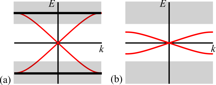
Figure 1: (a) If the spectral flow principle holds, there is a robust continuous attachment of anomalous boundary states (red) to a bulk band of delocalized states (black), which may be embedded in a wider bulk band of localizable states (grey). (b) Without spectral flow principle, anomalous surface bands (red) may in principle be detached from the bulk spectrum by a spectral gap or by band of Anderson localized states. In this case there is no obstruction to localization of the bulk states (grey). The figure shows a schematic one-dimensional boundary spectrum, assuming translation symmetry parallel to the boundary.

Physical properties of boundary states — such as their spatial structure at a given energy and the resulting conduction properties — are commonly addressed in terms of effective low-energy approaches that zoom in on linear crossing points in the boundary spectra. Employing such Dirac, or “${\bm{k}}\cdot{\bm{p}}$” approximations, physically relevant parts of the boundary spectrum are thus described by minimal models of manageable complexity. The anomalous nature of the boundary states — i.e., the fact that they do not exist as stand-alone lattice models — is reflected in the impossibility to close the Dirac theories in the limit of high momenta and exists for all tenfold-way classes. Nevertheless, as we show in detail for class AIII in three dimensions, absence of an ultraviolet closure of the surface Dirac theory does not automatically imply a continuous connection of the low-energy surface theory to the bulk spectrum.

Our work is motivated in part by a series of studies, which predicted — in contrast to the message of the present article — a spectrum-wide delocalization at the surface of class-AIII insulators and other tenfold-way classes with integer-valued invariants in three dimensions Ostrovsky et al. (2007); Ghorashi et al. (2018). That prediction was verified numerically as a robust feature of the effective two-dimensional Dirac surface theories of class CI, AIII, and DIII superconductors Ghorashi et al. (2018); Sbierski et al. (2020); Ghorashi et al. (2020); Karcher and Foster (2021), and it was backed up by numerical studies of a three-dimensional lattice model for class AIII Sbierski et al. (2020). On the other hand, robust topological arguments Essin and Gurarie (2015), or even rigorous mathematical proof Schulz-Baldes and Stoiber (2022) for surface state delocalization exist for states at zero energy only. With our demonstration that for class AIII all bulk states may be localized and that surface states can be energetically detached from the bulk, the spectrum-wide (de)localization of Refs. Ostrovsky et al. (2007); Ghorashi et al. (2018); Sbierski et al. (2020) is up for renegotiation. We will present numerical and analytical evidence that for a suitably chosen model realization all states away from zero energy are localized, albeit with a localization length diverging at zero energy.

To understand how these findings relate to the numerical results obtained previously, we have to anticipate some of the results derived in the remainder of this article. We there show that for an AIII insulator with winding number one — the “minimal” nontrivial topological insulator — perturbations interrupting the connection of the low-energy surface band of the class-AIII insulator to the bulk spectrum induce a surface Berry curvature in the surface band without breaking the chiral symmetry. This Berry curvature of the surface states is intimately tied to their localization behavior Altland et al. (2002): The surface states localize away from zero energy if the (spatially averaged) surface Berry curvature is nonzero, but not if it is zero. The spectrum-wide delocalization observed in Ref. Sbierski et al. (2020) therefore reflects a statistical symmetry of a model with zero average surface Berry curvature, not a topological obstruction to localization. On the other hand, a minimal two-dimensional Dirac theory with chiral symmetry — the two-dimensional surface theory that the numerical studies of Refs. Ghorashi et al. (2018); Sbierski et al. (2020); Ghorashi et al. (2020); Karcher and Foster (2021) were based on — is strictly without Berry curvature and, therefore, unable to capture the localizing geometric effects deriving from surface states at high energies.

The remainder of this article is organized as follows: In Sec. II we review the arguments relating delocalization of boundary states to the existence of (possibly high-energy) bulk states that are protected from localization in the Wigner-Dyson classes. Considering three-dimensional AIII as an example, we then discuss the principles which may lift this obstruction, and state the localizability status of all symmetry classes in dimensions up to three. In Sec. III we derive the same conclusions from the boundary perspective: We show that the effective Dirac-like surface theory of a class-AIII insulator is protected from being gapped at the special energy $E=0$, but not for $E\neq 0$, and that it may have nonzero Berry curvature at any energy $E\neq 0$. Both features may require the addition of trivial bands. (The minimal realization of the surface Dirac theory, on the other hand, cannot be gapped at any energy and has manifestly zero Berry curvature at all energies.) In Sec. IV we consider a canonical four-orbital topological-insulator lattice model for the class-AIII insulator in three dimensions Ryu et al. (2010), analogous to the model that was analyzed in Ref. Sbierski et al. (2020) to demonstrate spectrum-wide delocalization, and show that the surface bands can be detached from the bulk bands at a high energy by a suitably chosen perturbation. In Sec. V we present numerical evidence for surface localization if the average surface Berry curvature is nonzero and explain why delocalization is possible if surface regions with positive and negative Berry curvature occur with the same probability. We also discuss ramifications of our results for the experimental detection of 3D topological superconductors. Implications for the field-theoretic perspective are discussed in Sec. VI. We conclude in Sec. VII.

II Spectral flow: Bulk perspective

In the following, we will address the spectral flow principle from two different perspectives. The first, taken in this section, substantiates the connection between surface and bulk states alluded to in the introduction. In the next section we will then discuss spectral flow entirely on the basis of surface state physics.

II.1 Surface and bulk spectra

The spectral flow principle essentially relies on the topological equivalence of all surface states inside the bulk gap, irrespective of their energy. That the freedom to choose a reference energy inside the bulk gap implies the existence of a band of extended bulk states can be seen from a simple argument: Suppose, on the contrary, that for the bulk there exists a basis of (exponentially) localized eigenstates $|\Psi_{\mathbf{R}\alpha}\rangle$ at energies $\varepsilon_{{\mathbf{R}}\alpha}$ and with localization centers ${\mathbf{R}}$. (The index $\alpha$ is an additional index to label the eigenstates.) Then, up to an exponentially small correction, the Hamiltonian $H$ in the presence of a (possibly conducting) boundary can be written as the direct sum of boundary and bulk contributions Trifunovic (2020),

$$H=H_{\partial}\oplus H_{\rm bulk},$$ (1)

where $H_{\rm bulk}$ is the projection of $H$ onto eigenstates $|\Psi_{\mathbf{R}\alpha}\rangle$ with ${\mathbf{R}}$ farther than a cut-off distance from the boundary,

$$H_{\rm bulk}=\sum_{{\mathbf{R}}\in\textrm{bulk},\alpha}\varepsilon_{{\mathbf{R}}\alpha}|\Psi_{{\mathbf{R}}\alpha}\rangle\langle\Psi_{{\mathbf{R}}\alpha}|.$$ (2)

Because the eigenstates $|\Psi_{\mathbf{R}\alpha}\rangle$ are localized, $H_{\rm bulk}$ and, hence, $H_{\partial}$ are local operators. Choosing (without loss of generality) the Fermi energy at $E=0$ and defining $E^{\partial}$ and $E_{\rm gap}$ such that eigenvalues of $H_{\partial}$ and $H_{\rm bulk}$ are $\leq E^{\partial}$ and $\geq E_{\rm gap}$, respectively, see Fig. 2(a), $H$ may be continuously deformed to

$$H^{\prime}=\left(\frac{E_{\rm gap}}{2E^{\partial}}H_{\partial}\right)\oplus H_{\rm bulk},$$ (3)

which has a spectral gap for boundary and bulk for energies between $E_{\rm gap}/2$ and $E_{\rm gap}$, see Fig. 2(b), contradicting the requirement that a topological insulator must have conducting boundary states at all energies in the bulk gap.

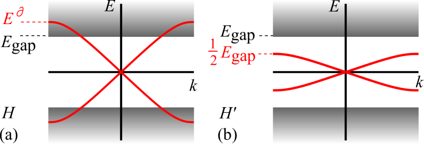
Figure 2: Schematic picture of surface (red) and bulk (black) spectra of a topological-insulator Hamiltonian $H$ (a) and the deformed Hamiltonian $H^{\prime}$ (b). If there exists a basis of localized eigenstates in the bulk, $H^{\prime}$ and $H$ are related via a continuous transformation.

The freedom to choose a reference energy inside the bulk gap exists for the three Wigner-Dyson classes A, AI, and AII, but not of the other tenfold-way symmetry classes. In these, the presence of charge-conjugation symmetry $\mathcal{C}$ and/or chiral symmetry $\mathcal{S}$ forces the spectrum to be mirror-symmetric around $E=0$. The equivalence of all energies inside the gap therefore no longer holds, and the spectral flow scenario must be reconsidered. Indeed, one may now argue in different directions, illustrated schematically in Fig. 1. One option is to say that deviations away from zero energy explicitly break the $\mathcal{C}$ or $\mathcal{S}$ symmetry in question, and so we are limited to statements of surface state delocalization at $E=0$. Indeed, this is as far as the rigorous mathematical proofs go Schulz-Baldes and Stoiber (2022). Alternatively, one may give the anomalous nature of the boundary states — which also holds for the non-Wigner-Dyson classes — priority and argue that these remain protected against acquiring a gap or being Anderson localized. However, from the simple argument presented after Eq. (1), a spectrum-wide protection of boundary states would necessarily imply the presence of a band of delocalized bulk states. We will consider the three-dimensional class AIII insulator as an example to demonstrate where this reading of a bulk-boundary correspondence can fail.

II.2 Case study: AIII insulator in three dimensions

The discussion above suggests that a continuous attachment of boundary states to the bulk spectrum and the existence of bulk delocalized states are flipsides of the same coin. The two-dimensional class A insulator is case in point for a situation where both exist. We now turn to the opposite situation, as realized in the three-dimensional AIII insulator, where spectral flow and delocalized bulk states are generically absent.

A Hamiltonian in class AIII can be written as

$$H =\begin{pmatrix}0&A\\ A^{\dagger}&0\end{pmatrix},$$ (4)

where $A$ is a complex square matrix acting on the subspaces defined by the condition $\Gamma=\pm 1$, and $\Gamma=\tau_{3}$ defines the chiral symmetry. For example, in a lattice system the subspaces corresponding to $\Gamma=\pm 1$ may define two bipartite sublattices. We assume that $H$ and, hence, $A$ are local matrices: The matrix elements $\langle{\mathbf{R}}\alpha|A|{\mathbf{R}}^{\prime}\alpha^{\prime}\rangle$ between atomic orbitals $\alpha$ and $\alpha^{\prime}$ at lattice sites ${\mathbf{R}}$ and ${\mathbf{R}}^{\prime}$ decay exponentially with the distance $|{\mathbf{R}}-{\mathbf{R}}^{\prime}|$.

For an insulator subject to periodic boundary conditions the spectrum of $H$ has a finite gap around zero energy. Hence, following Ref. Ryu et al. (2010), we may deform the Hamiltonian (4) by sending the positive (negative) eigenvalues of $H$ to $1$ ($-1$). Such a flattening deformation does not change the bulk topology and preserves the locality of the Hamiltonian matrix. It defines the Hamiltonian

$$H_{\textrm{f}} =\begin{pmatrix}0&U\\ U^{\dagger}&0\end{pmatrix}.$$ (5)

Locality of $H_{\rm f}$ implies that $U$ is a local unitary operator. ($U$ is unitary because $H_{\rm f}^{2}=\openone$.) We may then easily construct a basis of localized eigenstates at energy $\pm 1$ Read (2017),

$$|\Psi_{\mathbf{R}\alpha}^{\pm}\rangle=\frac{1}{\sqrt{2}}\begin{pmatrix}|\mathbf{R}\alpha\rangle\\ \pm U^{\dagger}|\mathbf{R}\alpha\rangle\end{pmatrix},$$ (6)

where $\alpha$ is an additional index. (Eigenstates $|\Psi_{{\mathbf{R}}\alpha}\rangle$ are localized near lattice site ${\mathbf{R}}$ because the unitary operator $U$ is local.) This simple construction proves the existence of a basis of localized eigenstates of $H_{\rm f}$, regardless of the underlyling topology . As shown by the argument presented around Eq. (1), localizability of the bulk Hamiltonian implies that surface and bulk spectra can be detached in principle.

For later reference we mention that the localized basis $\{|\Psi^{\eta}_{\mathbf{R}\alpha}\rangle\}$ and, hence, the decomposition of $H_{\rm f}$ into surface and bulk contributions as in Eq. (1) is not unique: Each local unitary matrix $V$ generates another localized basis $\{|\Psi^{\eta,V}_{\mathbf{R}\alpha}\rangle\}$ by multiplying both elements of the two-component spinor in Eq. (6) by $V$. In Sec. IV.3, we demonstrate that the surface states described by $H_{\partial}$ in Eq. (1) may have a nonzero Chern number Ch. This number is constrained to have the same parity as the winding number of the bulk Hamiltonians $H$ and $H_{\rm f}$. However, for a given parity its value depends on the choice of the localized basis for the bulk states: basis changes $|\Psi^{\eta}_{\mathbf{R}\alpha}\rangle\to|\Psi^{\eta,V}_{\mathbf{R}\alpha}\rangle$ lead to a change Lapierre et al. (2021)

$$\delta\text{Ch} =2W[V],$$ (7)

where, for a periodically extended definition of the local transformation, $W[V]\in\mathbb{Z}$ is the third winding number of $V$ over momentum space. (An analogous relation was found for the surface response theory of a three-dimensional topological insulator Qi et al. (2008).)

II.3 Other tenfold-way classes

class	$\,d=1$	$d=2$	$d=3$
A	$0$	$\mathbb{Z}^{\checkmark}$	$0$
AIII	$\mathbb{Z}^{\times}$	$0$	$\mathbb{Z}^{\times}$
AI	$0$	$0$	$0$
BDI	$\mathbb{Z}^{\times}$	$0$	$0$
D	$\mathbb{Z}_{2}^{\times}$	$\mathbb{Z}^{\checkmark}$	$0$
DIII	$\mathbb{Z}_{2}^{\times}$	$\mathbb{Z}_{2}^{\checkmark}$	$\mathbb{Z}^{\checkmark/\times}$
AII	$0$	$\mathbb{Z}_{2}^{\checkmark}$	$\mathbb{Z}_{2}^{\checkmark}$
CII	$2\mathbb{Z}^{\times}$	$0$	$\mathbb{Z}_{2}^{\times}$
C	$0$	$2\mathbb{Z}^{\checkmark}$	$0$
CI	$0$	$0$	$2\mathbb{Z}^{\times}$

Table 1: Localizability of topological insulators and superconductors. The absence of topological phase is denoted by $0$, whereas entries where topological phases exist are labeled by “$\times$” for localizable and “$\checkmark$” for non-localizable phase. For class DIII in three dimensions, superconductors with even bulk invariant are localizable, whereas superconductors with odd bulk invariant are non-localizable. The spectral flow principle only applies to non-localizable classes (denoted with $\checkmark$).

The discussion above shows that there are two different classes of topological insulators: those with and without a spectral flow principle. Given that this dichotomy presides over the spectrum-wide robustness of boundary states, it seems necessary to tag each entry in the periodic table of topological insulators and superconductors Kitaev (2009); Schnyder et al. (2008); Ryu et al. (2010) according to its localizability status. Referring for the full classification program to the upcoming publication , Table 1 summarizes the result for dimensions up to three. It adds to the topological status of a given symmetry class and dimensionality ($\mathbb{Z},\mathbb{Z}_{2}$, or $0$) information on the localizability of its states: The absence of topology is denoted by the entry “$0$,” topological classes with symmetry-compatible exponentially localizable bulk states are labeled by “$\times$,” and those with not fully localizable bulk by “$\checkmark$.”

Localizability or, as is is often called in the literature, Wannierizability Thouless (1984); Brouder et al. (2007); Thonhauser and Vanderbilt (2006); Soluyanov and Vanderbilt (2011); Winkler et al. (2016); Cornean et al. (2017), is not the same as being deformable to an “atomic limit”. The requirement that bulk states can be exponentially localized is essential here: A stronger requirement, e.g., that there exists a basis of bulk states with compact support leads to a trivial classification for dimensions $d>1$ Read (2017). An “atomic-limit” insulator has eigenstates that can be localized inside unit cell. For the topologically nontrivial non-Wigner-Dyson classes, there still is an obstruction to localizing the eigenstates inside a unit cell, which is consistent with the presence of anomalous delocalized boundary states, in spite of the bulk bands being localizable.

The information provided by Tab. 1 confirms the argument formulated at the beginning of this section: topological classes without $\mathcal{C}$ or $\mathcal{S}$ symmetries, i.e., A, AI, and AII, are not localizable. For the non-Wigner-Dyson classes, what determines localizability is whether $\mathcal{C}$ or $\mathcal{S}$ are essential for the topology, or whether they are “spectator symmetries” and the topology of the bulk Hamiltonian remains nontrivial if all constraints imposed by $\mathcal{C}$ and/or $\mathcal{S}$ are lifted. In three dimensions, class AIII is an example of the former category, which we refer to as “genuine” non-Wigner-Dyson classes. Other examples of “genuine” non-Wigner-Dyson classes are classes BDI and D in one dimension and classes CI and CII in three dimensions. Examples of “non-genuine” non-Wigner-Dyson classes are classes C and D in two dimensions, which have chiral edge states Senthil and Fisher (2000); Read and Green (2000), and which remain topological if the particle-hole symmetry is lifted. Class DIII in three dimensions, which describes time-reversal-invariant superconductors with broken spin-rotation symmetry is a special case, as it is a localizable “genuine” non-Wigner-Dyson class only if the topological invariant is even.

The existence of a localized basis for the one-dimensional topological tenfold-way classes (second column in Table 1) is well known in the literature Kohn (1959). Example are the Su-Schrieffer-Heeger model (class AIII) Su et al. (1979); Kivelson (1982); Bradlyn et al. (2017) and the topological superconductor (class D, the “Kitaev chain” Kitaev (2001)), which in their nontrivial phase have localized bases that stretch across adjacent unit cells. The possibility of localizable topological superconductors in dimensions larger than one was mentioned by Ono, Po, and Watanabe Ono et al. (2020) in the context of topological superconductors with additional crystalline symmetries (see also Ref. Zhang et al. (2020)).

Since bulk localizability implies the breakdown of the spectral flow argument, we expect that boundary states away from $E=0$ will be localizable, too. However, “localizable” does not automatically mean “localized.” The considerations of this Section therefore raise the follow-up question how the localizability of surface states relates to the recent observations of delocalized surface spectra in classes AIII or CI Karcher and Foster (2021), and to the remarkable resilience of two-dimensional Dirac surface theories to localization. In the rest of the paper we provide answers to these questions for our principal case study, three-dimensional AIII.

III Spectral-flow: Boundary perspective

In the previous section, we considered the status of surface states on the basis of a connection to bulk states via the spectral flow correspondence. We here approach the question from a complementary perspective, which focuses entirely on the surfaces themselves.

III.1 General considerations

The vicinity of the Fermi crossing points at topological insulator surfaces is often described in terms of effective Dirac Hamiltonians, which in the two-dimensional case assume the form

$$H_{\textrm{b}}=k_{1}\Gamma_{1}+k_{2}\Gamma_{2},$$ (8)

where $k_{i}$ are two momenta along the surface measured relative to the crossing point ${\bm{k}}=0$, and the two Gamma matrices satisfy $\{\Gamma_{1},\Gamma_{2}\}=\delta_{ij}$. Additional Gamma matrices may appear at higher order in $k$ or as prefactors of a random surface potential. At large momenta, the Hamiltonian (8) is ultraviolet divergent. These divergences cannot be cured by embedding $H_{\textrm{b}}$ into the periodic structure of a two-dimensional Brillouin zone, reflecting that the surface theory does not define the low-energy limit of a two-dimensional stand-alone lattice model.

In the context defined by Eq. (8), the spectral flow principle translates to the statement of an anomaly: Coupled to an external vector potential, $H_{\textrm{b}}$, supplemented with an ultraviolet regularization, lacks gauge invariance. The absence of gauge invariance indicates (quasi-)particle number non-conservation. Specifically, under adiabatic insertion of a flux quantum through the bulk, high-lying boundary states get pushed up in energy, leading to a drain out of the window of momentum states below a fixed cutoff. If the spectral flow principle applies, overall particle number conservation is restored by conversion of boundary states into bulk states and eventually to states at the opposite surface. The observable consequence is adiabatic transport from one boundary to the other, i.e., the quantized transverse conductance characteristic of topological insulators.

In the previous Section, we have argued that the spectral flow principle does not apply to all symmetry classes. How can this be reconciled with the intrinsic absence of an ultraviolet closure of the Dirac surface theory? To resolve the anomaly of the latter there must exist a “sink” of high-lying states absorbing spectral weight being pushed up by an anomalous gauge operation. If the spectral flow principle applies, these are extended bulk states. If it does not apply, implying that the boundary states can be detached from the bulk, these states must be supported by the boundaries themselves.

In the following we illustrate these complementary scenarios on two case studies, class A in two, and class AIII in three dimensions. In either case, the focus will be entirely on the boundaries, no explicit reference to bulk states is made.

III.2 Case study: Class-A Chern insulator in two dimensions

Two-dimensional class A is the paradigmatic example of an insulator with spectral flow, as realized, e.g., in the physics of the integer quantum Hall effect. In this case, the boundary theory (linearized around any Fermi energy) is governed by the effective Hamiltonian

$$H_{\textrm{b}}=k,$$ (9)

describing a single branch of chiral fermions.

Assuming zero temperature, and the Fermi energy at $E=0$ for convenience, states with $k<0$ are occupied. Coupling the system to a gauge potential representing adiabatic magnetic flux insertion through the bulk, $k\to k+A$, causes an upward shift of all levels. After the insertion of one flux quantum, the full quantized single particle spectrum is restored, but the occupations of the states have changed, as shown schematically in Fig. 3(a). Specifically, one occupied state previously at $k<0$ now occupies the lowest state at $k>0$. By repeated insertion of flux quanta, the range of occupied states will extend up to arbitrarily high energies and, eventually, a state previously sitting at the upper cutoff of the low-energy theory gets pushed beyond it [see the arrows in Fig. 3(a)].

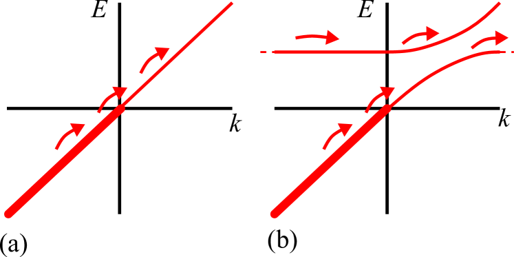
Figure 3: Schematic dispersions of the minimal edge Hamiltonian (9) (a) and of the non-minimal model (10), which has an additional band of localized states at the edge (b). Since it derives from a lattice model, the asymptotically flat band from the localized states must be continuously connected for $k\to\infty$ and $k\to-\infty$, to reflect the periodicity of the edge Brillouin zone. Unbounded bands are continuously connected to the bulk spectrum for $k\to\infty$ and $k\to-\infty$. The arrows indicate how the occupation of states is changed after insertion of a flux quantum through the bulk.

Topological features must be stable with respect to arbitrary perturbations at the boundary. To see how this robustness manifests itself in the anomaly of the boundary Hamiltonian (9), consider adding a band of trivial localized boundary states at energy $\varepsilon_{\mathrm{c}}>0$. Assuming weak coupling $\gamma$ to the chiral band, the boundary Hamiltonian generalizes to

$$H_{\textrm{b}}^{\prime}=\begin{pmatrix}k&\gamma\\ \gamma^{*}&\varepsilon_{\rm c}\end{pmatrix}.$$ (10)

The coupling matrix element $\gamma$ now generates an avoided crossing between the chiral and the flat band, see Fig. 3(b), and a local gap close to the momentum $k\sim\varepsilon_{\mathrm{c}}$ . However, the global spectrum of the boundary Hamiltonian remains gapless, the reason being that the band structure of the localized states must be continuous throughout the boundary Brillouin zone. For the same reason, the addition of the localized band does not resolve the ultraviolet anomaly of the boundary theory. Indeed, if flux quanta are inserted repeatedly through the bulk, the occupied states will eventually completely fill the flat band of localized boundary states and continue to reach the upper cutoff [see arrows in Fig. 3(b)].

We now turn to three-dimensional class AIII and discuss how a construction similar to the one above leads to very different conclusions.

III.3 Case study: Class AIII insulator in three dimensions

The minimal surface theory of a class AIII insulator with winding number one described by a two-dimensional generalization of Eq. (9),

$$H_{\textrm{b}}=k_{x}\tau_{1}+k_{y}\tau_{2}.$$ (11)

where the chiral symmetry is realized as $H_{\textrm{b}}=-\Gamma H_{\textrm{b}}\Gamma$ with $\Gamma=\tau_{3}$. Again, this Hamiltonian has no ultraviolet closure. (To see why, note that the off-diagonal element $k_{x}-ik_{y}$ defines a winding number around the origin in two-dimensional $k$-space. This is incompatible with the $k$-space periodicity required by a genuine two-dimensional lattice Hamiltonian.)

A continuous deformation of this two-band Hamiltonian cannot open a gap at zero energy. The required perturbation would have to be proportional to $\tau_{3}$, in violation of the chiral symmetry. The conduction and valence band then connect the single touching point ${\bm{k}}=\mathbf{0}$ to the ultraviolet divergences at large momentum; Within this two-band representation, the dispersion is continuous without gap openings at finite momenta. It is for this Hamiltonian, augmented with a chiral symmetry respecting random vector potential, that Refs. Ghorashi et al. (2018); Sbierski et al. (2020); Karcher and Foster (2021) established a spectrum-wide resilience to Anderson localization.

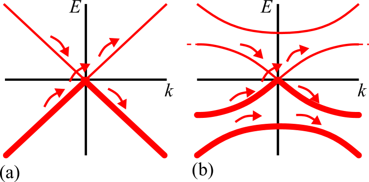
Figure 4: Schematic dispersions of the minimal edge Hamiltonian (11) (a) and the non-minimal model (12), which has two additional bands of localized states at the edge (b). The asymptotically flats band from the localized states must be continuously connected for $k\to\infty$ and $k\to-\infty$, to reflect the periodicity of the edge Brillouin zone. The ultraviolet divergent bands from the chiral edge states are continuously attached to the bulk spectrum for $k\to\infty$ and $k\to-\infty$. In the non-minimal model, the high-energy band is detached from the low-energy band containing the linear crossing at zero energy. The arrows indicate how the occupation of states is changed after insertion of a flux quantum through the bulk.

As in our previous discussion of class A, we now introduce a band of localized surface states at energies $\pm\varepsilon_{\rm c}$. As a two-dimensional surface Hamiltonian analogous to Eq. (10) we consider

$$H_{\textrm{b}}^{\prime}=\begin{pmatrix}k_{x}\tau_{1}+k_{y}\tau_{2}&\gamma\tau_{-}\\ \gamma^{*}\tau_{+}&\varepsilon_{\rm c}\tau_{1}\end{pmatrix},$$ (12)

where $\tau_{\pm}=\tau_{1}\pm i\tau_{2}$. As in class A, the band-coupling $\gamma\tau_{-}$ defines an avoided crossing between the localized and the linearly dispersive bands, see Fig. 4(b). However, unlike in class A, the continuous interpolation of the bands at the boundaries of the Brillouin zone no longer presents an obstruction to the opening of a global gap, see Fig. 4(b). This option to disrupt the surface spectrum was to be expected from the discussion of bulk state localizability in Sec. II, but here follows from inspection of the surface alone.

We note that the Hamiltonian (12) still has, and needs to have, an ultraviolet divergence. However, unlike in class A the repeated insertion of bulk flux quanta no longer leads to a spectral flow anomaly: the occupied states get shifted as indicated by the arrows in Fig. 4(b), and eventually fill the large-$k$ part of band of localized boundary states. However no particles reach the upper energy cut-off. This observation indicates that the ultraviolet divergence of effective surface Hamiltonians — which reflects their non-existence without a supporting bulk — does not necessarily imply spectral flow from the surface into the bulk.

In the literature, topological properties that are robust to the addition of trivial bands are called “stable”. The sensitivity of the minimal model to the addition of bands, i.e., the opening of gaps and the disruption of spectral flow, should therefore be considered a manifestation of “unstable” or “fragile” topology: the conclusion is that minimal models are insufficient to fathom the full spectrum of phenomenologies displayed by the surfaces of three-dimensional AIII insulators.

Although the concrete worked-out example here is for an AIII insulator with winding number $\nu=1$, the general conclusion about the fragility of the spectrum-wide protection of the surface bands in a minimal effective $2\times 2$ theory equally applies to higher winding numbers. A $2\times 2$ surface theory with a winding number larger than one may be realized as a nodal point involving higher powers of the momentum ${\bm{k}}$ or by having multiple nodal points at different locations in reciprocal space. In either case, the restriction to two-component spinors precludes the interruption of the surface states by a spectral or mobility gap.

Below Eq. (11), we linked the absence of intrinsic UV regularization of effective surface theories to the presence of a winding number. It is interesting to observe that the isolation of detached surface band introduces another invariant, namely a two-dimensional surface Chern number. Describing the momentum space topology of the band through the map ${\bm{k}}\to|\alpha_{\bm{k}}\rangle$, where ${\bm{k}}$ runs through the two-dimensional Brillouin zone, and $|\alpha_{\bm{k}}\rangle$ are the positive energy states of the finite band indicted in Fig. 4b, we define the Berry curvature

$$\Omega_{\bm{k}}=i\langle d\alpha_{\bm{k}}|\wedge d\alpha_{\bm{k}}\rangle,$$ (13)

and from it the Chern number,

$$\textrm{Ch}\equiv\frac{1}{\pi}\int_{\mathrm{BZ}}\Omega_{\bm{k}}.$$ (14)

This is the surface Chern number mentioned previously in section II.2. While its numerical value may vary depending on the realization of the coupling between the trivial and the chiral bands, its parity is determined by that of the bulk winding number. For further discussion of this point, we refer to section IV.3.

IV AIII insulator in three dimensions

In the previous section we discussed generic features of topological insulator bulk states and of their asymptotically linearizable surface spectra. We will now turn to a more concrete level and discuss the band structure of a microscopic model in class AIII. In the next section we then generalize to the presence of static disorder and discuss localization properties of the model’s surface states.

We start our discussion with the definition of the model in subsection IV.1. Following standard protocol, we then project down to its low-energy Dirac approximation in subsection IV.2. [Impatient readers may just take notice of the two principal definitions (17) of the lattice model and (25) of its Dirac approximation, and directly proceed to Sec. IV.3.] On the basis of these model definitions we then discuss spectral flow in sections IV.3-IV.4.

IV.1 Lattice model

We consider a cubic lattice model with four orbitals per site defined by the Bloch Hamiltonian Ryu et al. (2010)

$$H({\bm{k}})= \,\left(M-\sum_{a=1}^{3}\cos k_{a}\right)\tau_{2}\sigma_{0}+\sum_{a=1}^{3}\tau_{1}\sigma_{a}\sin k_{a},$$ (15)

where we set the hopping strength, which is parametrically of the same order as the total band width, to unity for convenience. The Pauli matrices ${\sigma}_{\mu}$ and ${\tau}_{\mu}$ act on two independent degrees of freedom of the $4=2\times 2$ orbitals in the unit cell. An application of the standard mapping Ryu et al. (2010) between chiral lattice Hamiltonians and three-dimensional winding number invariants, $W$, shows that

$$\left.\begin{array}[]{l}W=1\cr W=-2\cr W=0\end{array}\right\}\qquad\textrm{for}\qquad\left.\begin{array}[]{l}1<|M|<3\cr|M|<1\cr\textrm{else}\end{array}\right\}.$$

The Hamiltonian (15) is invariant under the symmetry operations $\mathcal{S}$ and $\mathcal{C}$, with $\mathcal{C}^{2}=-1$,

$$H({\bm{k}})= \,-M_{\mathcal{S}}\,H({\bm{k}})\,M_{\mathcal{S}}$$

$$= \,-M_{\mathcal{C}}\,H^{\mathsf{T}}({\bm{k}})\,M_{\mathcal{C}}.$$ (16)

Here $\mathsf{T}$ denotes the matrix transpose, $M_{\mathcal{S}}=\tau_{3}$, and $M_{\mathcal{C}}=\tau_{2}\sigma_{2}$. We note that the combination $\mathcal{C}\mathcal{S}=\mathcal{T}$ of charge-conjugation and chiral symmetry satisfies $\mathcal{T}^{2}=-1$, putting our system into class DIII .

To define a class AIII model, we break $\mathcal{C}$, while preserving $\mathcal{S}$. For our purposes, it will be convenient to realize this symmetry breaking by adding $\mathcal{C}$-breaking disorder. To this end, we turn to a real space representation of the model (15), which reads

$$H=H_{0}+\sum_{a=1}^{3}H_{a},$$ (17)

with

$$H_{0}= \,M\sum_{{\mathbf{R}}}|{\mathbf{R}}\rangle\tau_{2}\sigma_{0}\langle{\mathbf{R}}|,$$ (18)

$$H_{a}= \,\frac{1}{2}\sum_{{\mathbf{R}}}\Big{[}t_{{\mathbf{R}}}^{a}|{\mathbf{R}}+{\bm{e}}_{a}\rangle(\tau_{2}\sigma_{0}-i\tau_{1}\sigma_{a})\langle{\mathbf{R}}+{\bm{e}}_{a}|+\mbox{h.c.}\Big{]},$$

where the ${\mathbf{R}}$ are lattice vectors on the cubic lattice, and the $\mathbf{e}_{a}$, $a=1,2,3$ unit vectors in the lattice directions. The amplitudes $t_{{\mathbf{R}}}^{a}$, constant in the clean case, are now chosen as,

$$t_{{\mathbf{R}}}^{a}\rightarrow t\,e^{-i\phi^{a}_{\bm{\mathrm{R}}}},$$ (19)

where $a\in\{1,2,3\}$ specifies the direction of the nearest-neighbor bond, and the $\{\phi^{a}_{\bm{\mathrm{x}}}\}$ are static random phase variables with variance 

$$\langle\phi_{\mathbf{R}}^{a}\phi_{\mathbf{R^{\prime}}}^{a^{\prime}}\rangle=W^{2}\delta_{\mathbf{R}\mathbf{R}^{\prime}}\delta_{aa^{\prime}}.$$ (20)

The effects of this disorder on the (de)localization properties of the surface states will be discussed in Sec. V.

IV.2 Surface Dirac approximation

A bulk winding number $W$ generically implies the appearance of $|W|$ species of gapless Dirac fermions at the surface Ryu et al. (2010). Specifically, we consider a $W=1$ realization of the model (15) with $1<M<3$, a vacuum interface at $x=0$ in the 1-direction, and infinite extension in $2$- and $3$-directions. In this case, a Dirac surface state appears in the surface Brillouin zone at $(k_{2},k_{3})=(0,0)$.

Considering $\mu\equiv 3-M$, with $0<\mu\ll 1$, a continuum approximation near the bottom of the band leads to the effective Hamiltonian

$${H}\simeq \,{H}_{0}+{H}_{1},$$ (21)

with

$${H}_{0}= \,\left(-\frac{1}{2}\frac{d^{2}}{dx^{2}}-\mu\right){\tau}_{2}{\sigma}_{0}+{\tau}_{1}{\sigma}_{1}\left(-i\frac{d}{dx}\right),$$ (22)

$${H}_{1}= \,\left(\frac{k_{2}^{2}+k_{3}^{2}}{2}\right){\tau}_{2}{\sigma}_{0}+k_{2}\,{\tau}_{1}{\sigma}_{2}+k_{3}\,{\tau}_{1}{\sigma}_{3}.$$ (23)

The zero modes of ${H}_{0}$ are

$$|0,m\rangle\equiv|m_{z}\rangle_{\tau}|m_{x}\rangle_{\sigma}|\psi\rangle,$$ (24)

where $m\in\{\uparrow,\downarrow\}$ denotes the polarization of the surface state, and $|\psi\rangle$ is an envelope function decaying exponentially into the bulk in the $x$-direction. The projection of the transverse part of the Hamiltonian ${H}_{1}$ into the space of zero modes gives

$${H}_{1}\rightarrow\begin{pmatrix}0&k_{3}-ik_{2}\\ k_{3}+ik_{2}&0\end{pmatrix}=\bm{\mathrm{k}}\cdot\bm{\mathrm{\Gamma}},$$ (25)

where $\bm{\mathrm{k}}\equiv\{k_{3},k_{2}\}$ and ${\bm{\mathrm{\Gamma}}}=\{{\Gamma}_{1},{\Gamma}_{2}\}$ are the standard Pauli matrices acting in the space of zero modes.

Equation (25) defines the minimal two-component massless Dirac approximation to the surface states of the bulk model in Eq. (15) with winding number $W=1$. As discussed in Sec. III, the minimal Dirac surface theory has a fragile obstruction to localization, which is lifted if additional degrees of freedom are added to the surface theory. In Sec. III the additional degrees of freedom were added in the form of a trivial band of localized states at the surface. In the next subsections, we will show that the inclusion of the quantum geometric structure of the high-lying states in the full three-dimensional theory has the same effect.

IV.3 Detaching bulk and surface bands

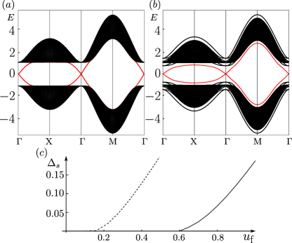
Figure 5: (a) Spectrum of the topological insulator (15) with $M=2$ for open boundary conditions the $x$-direction. The bulk (surface) spectrum is shown in black (red). There is a single low-energy Dirac cone at $(k_{y},k_{z})=\Gamma=(0,0)$. Surface and bulk bands merge at high energy. (b) The same as panel (a) but with the additional perturbation $U_{\rm f}$ of Eq. (26) with $u_{\rm f}=0.5$ and $n=3$. (c) Minimal value of the strength $u_{\rm f}$ of the fragmenting potential (26) required to detach surface and bulk bands, for a perturbation with support on the outermost surface layer only ($n=1$, solid) and for a perturbation with support on the three outermost surface layers ($n=3$, dashed). The vertical axis shows the minimal value of the indirect gap $\Delta_{\rm s}$ between surface and bulk bands.

The model (15) has a surface band that is continuously connected to the bulk, see Fig. 5(a). We add a term

$$U_{\rm f} =\sum_{{\mathbf{R}}\in\textrm{surface}}u_{\rm f}({\mathbf{R}})|{\mathbf{R}}\rangle{\tau}_{2}\,{\sigma}_{1}\langle{\mathbf{R}}|,$$ (26)

where we set $u_{\rm f}({\mathbf{R}})=u_{\rm f}$ nonzero for ${\mathbf{R}}$ in the $n$ outermost surface layers, and $u_{\rm f}({\mathbf{R}})=0$ otherwise. (We set $n=1$ or $n=3$ in our numerical calculations.) The perturbation $U_{\rm f}$ breaks $\mathcal{C}$ and $\mathcal{T}=\mathcal{C}\mathcal{S}$ symmetries, but preserves $\mathcal{S}$. We refer to this perturbation as “fragmenting surface potential”. The definition of the fragmenting potential (26) depends on the surface orientation and transforms the same way as the low-energy surface Dirac cone (25). For values $u_{\rm f}>u_{\rm f}^{\rm c}$, we observe the opening of an indirect global gap between the surface band and bulk bands, see Fig. 5(b). The threshold parameter $u_{\rm f}^{\rm c}$ depends on how many surface layers are perturbed by the fragmenting surface potential, see Fig. 5(c). However, regardless of its concrete value, the present construction demonstrates the interruptibility of spectral flow.

For later reference, we mention that the question whether or not states in a surface band with winding number one (as is the case for the model we investigate here) are localized at energy $E$ can be answered by considering the integrated Berry curvature carried by the states with energy $\varepsilon_{k}$ between $0$ and $E$. Hereto we define

$$\theta(E)=\pi+\int_{0\leq\varepsilon_{{\bm{k}}}\leq E}\Omega_{{\bm{k}}}.$$ (27)

The field theoretical analysis of such a system in the presence of disorder, see Sec. VI, then shows that states are delocalized at energy $E$ if

$$\theta(E)=\pi\mod 2\pi.$$ (28)

Since $\theta(0)=\pi$, this condition is consistent with the topological surface states at $E=0$ being delocalized.

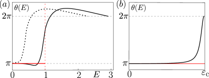
Figure 6: (a) Integrated Berry curvature $\theta(E)$ of the surface band of the model (15) vs. energy $E$ for the case of zero fragmenting potential $u_{\rm f}$ (red), $u_{\rm f}=-0.3$ (black, solid), and $u_{\rm f}=-1$ (black, dotted). The fragmenting potential is added on the three outermost layers adjacent to the surface, $n=3$. The vertical red lines denote the position of the bulk gap. For the two nonzero values of $u_{\rm f}$, surface and bulk band are detached, so that $\theta(E)$ can be determined for the full surface band; for $u_{\rm f}=0$, $\theta(E)$ can be calculated only for energy $E$ inside the bulk gap. (b) The same as panel (a) but for the minimal surface theory (11) (red) and the non-minimal model (12) (black) with $|\gamma|/\varepsilon_{\rm c}=0.05$. According to the criterion of Ref. Moreno-Gonzalez et al. (2023), surface states at energy $E$ are delocalized if $\theta(E)=\pi\mod 2\pi$.

Fig. 6(a) shows the angle $\theta(E)$ as a function of $E$ for $u_{\rm f}=0.3$ and $u_{\rm f}=1.0$ and with the fragmenting perturbation supported on the three outermost layers ($n=3$). We note that the presence of $u_{\rm f}$ has little effect for energies close to $E=0$ . This is consistent with the absence of Berry curvature in the two-component Dirac approximation, which in turn is a consequence of the chiral symmetry (i.e. the absence of terms on the diagonal of the $2\times 2$ matrix operator.) However, we observe significant deviations from $\theta(E)=\pi$ for energies approaching the edges of the bulk bands. In the light of our discussion of section III.3, these reflect the onset of effective hybdridization with extraneous bands, whose role in the present context is assumed by the bulk bands.

For comparison, in Fig. 6(b) we also show $\theta(E)$ for the two-dimensional band that was obtained by coupling a surface Dirac cone to a localized surface band, see Eq. (12). Analogous to the detached surface band of the full 3d model shown in Fig. 6(a), the Berry curvature is concentrated mainly near the band edges.

We finally note that the integral of the Berry curvature over the entire surface band gives the Chern number Ch of the surface band. Its numerical value depends on the sign of the fragmenting potential,

$$\text{Ch}=-\text{sign}(u_{\rm f}).$$ (29)

Comparing the above result with Eq. (7), we conclude that the sign of $u_{\rm f}$ corresponds to two different bulk gauge choices for the detachment of surface and bulk. Alternatively, comparing with the phenomenological surface theory (12), different signs of $u_{\rm f}$ represent different perturbations coupling the dispersing surface band and the degrees of freedom of the external band.

IV.4 Chiral-symmetric chiral modes: surface Hall conductance

We have seen that addition of the perturbation (26) detaches the surface bands from the bulk and that the now isolated surface band has a nonzero Chern number Ch, which for the present $\nu=1$ model is given by Eq. (29). It is interesting to ask what happens if $u_{\rm f}$ changes sign, for example along an intra surface domain wall. As we will see, the ensuing phenomenology is key to the understanding of the disordered system below.

To explore this situation in the simplest possible setting, we consider a flattened version of the model (15). The latter is obtained from the Hamiltonian (15) by keeping its Bloch states unchanged, while sending the energy eigenvalues to $\pm 1$. To describe an insulator with a surface, we then switch to the position representation and impose open (or vacuum) boundary conditions at two coordinates in $x$-direction. More specifically, we consider an annular cylinder geometry with two surfaces in the radial $x$-direction, periodic boundary conditions in circumferential $y$-direction, and the cylinder axis in $z$-direction.

Figure 7 shows that for a constant mass (26), the flattened model shows a global gap between surface (red) and flat bulk (black) bands. However, the spectrum becomes more interesting, once we introduce two surface domain walls parallel to the $z$-direction where $u_{\rm f}$ switches sign. (Periodicity in $y$-direction requires the presence of two of these.) In this case, we observe the formation of two counterpropagating chiral modes bound to the respective domain walls. The spectrum of these modes, indicated in green in Figure 7(a) connects the surface and the bulk spectrum.

In the clean model, these chiral modes are supported only by states inside the high-lying band gap. Below it, they hybridize with the extended surface states. In the presence of disorder, the surface states at $E\neq 0$ will localize, but the chiral edge modes do not, so that, for sufficiently strong disorder, the chiral modes will eventually extend their support over the entire surface spectrum, cf. Fig. 7 (b).

At energies $E\neq 0$ the chiral symmetry is effectively broken, so that we may think of each surface as a two-dimensional system in class A. In this reading, the counterpropagating chiral modes at the domain walls surrounding a surface region with a different sign of the fragmenting potential acquire a status equivalent to the edge modes of a quantum Hall insulator, and Laughlin’s gauge argument applies. It requires that the branches of chiral modes must eventually hybridize with extended states, at $E=0$ as well as at high energies. The extended states at $E=0$ are the topologically protected delocalized surface states of the class-AIII insulator. At high energies, the chiral modes must hybridize with delocalized bulk states or with energetically high-lying delocalized surface states. Either way, the presence of the domain wall modes prevents a full localizability of all states at large energies.

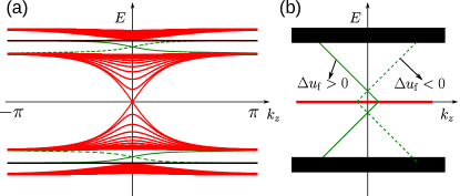
Figure 7: (a) Band structure for a slab geometry of the flattened version of the model (15) with open boundary conditions along $x$ and two symmetrically placed domain walls and periodic boundary boundary conditions along $y$. The domain-wall height $\Delta u_{\rm f}$ takes the values $\pm 0.2$ and has support in $n=1$ layer closest to the surface. The bulk, surface, and domain-wall part of the spectrum are indicated in black, red, and green, respectively. Solid and dashed green curves are for the domain wall for which $u_{\rm f}$ goes from negative to positive and from positive to negative upon increasing $y$, respectively. Note that the addition of the fragmenting potential to the surface raises part of the surface spectrum above the flattened bulk band. (b) In the presence of disorder, only surface states at $E=0$ are delocalized. In this case, the chiral domain-wall modes are expected to extend from the bulk spectrum all the way down to zero energy.

In anticipation of our later in-depth discussion of disorder, it will be rewarding to link the presence of chiral edge modes to transport coefficients. To this end, consider a surface geometry where a puddle of given value of $u_{\rm f}$ is surrounded by an outer region with $u_{\rm f}$ of opposite sign. The presence of a chiral edge mode at the puddle boundary implies that a fictitious four-terminal measurement of its Hall conductance would yield the result $\sigma(E)=\mathrm{sgn}(E)\,\mathrm{sgn}(u_{\rm f})/2$ for all energies inside the mobility gap where the chiral mode exists. (The factor $1/2$ reflects the fact that the surface is governed by a single Dirac fermion species, with its characteristic half-integral transverse conductance. Chiral symmetry requires $\sigma(E)$ to be an odd function of $E$ Trifunovic and Brouwer (2019). At the band center, $\sigma(0)=0$, again by chiral symmetry.).

Now imagine a mass profile $u_{\rm f}(y,z)$ smoothly varying in such a way that the spatial average $\langle u_{\rm f}(y,z)\rangle=0$ and puddles with masses of opposite sign form with equal probability. Since each puddle is surrounded by its own chiral mode, we expect the formation of a network in which co- and counterpropagating loops occur with equal likelihood. This system is topologically equivalent to the Chalker-Coddington network Chalker and Coddington (1988) of the integer quantum Hall effect at criticality. At this point, the network model predicts the percolation of quantum states evading Anderson localization in the presence of even strong disorder. This simple picture — which is the mechanism behind the “statistical topological insulator” Fulga et al. (2014) — is compatible with the observation of model realizations with a spectrum-wide existence of delocalized surface states Sbierski et al. (2020). (The same statistical mechanism underlies delocalization of a topological-insulator surface in a random magnetic field Nomura et al. (2008) and of the surface states of a weak topological insulator Ringel et al. (2012); Mong et al. (2012); Fu and Kane (2012).) On the other hand, we expect localization of finite-energy surface states if a non-vanishing average $\langle u_{\rm f}(y,z)\rangle\neq 0$ causes an imbalance between puddles with opposite signs of $u_{\rm f}$. Note that these predictions are consistent with the expectation that it is the presence or absence of Berry curvature, corresponding to the presence or absence of an average surface fragmenting potential, that decides over localization. In the next section, we will back these hypotheses by a quantitative analysis of disorder.

V Surface localization properties

Previous sections demonstrated that the surface states of a class AIII topological insulator can be detached from the bulk. Concomitant with the opening of the spectral gap, the 2D surface acquires a nonzero Chern number due to induced surface Berry curvature, as explicated above in Secs. III.3 and IV.3.

In this section, we consider the implications of surface Berry curvature for the Anderson localization properties of the surface states in the presence of symmetry-preserving disorder. Since the minimal 2-component surface Dirac theory is void of curvature, we work with a slab of the 3D lattice model defined in Eq. (17). Surface Berry curvature is induced along the slab boundary via the fragmenting potential introduced in Eq. (26), above.

We demonstrate below (see Fig. 8) that a nonzero uniform fragmenting potential localizes all surface states except the zero-energy one, which remains topologically protected. By contrast, spectrum-wide criticality (critical delocalization linked to the plateau transition of the quantum Hall effect Sbierski et al. (2020)) survives when either (a) the surface fragmenting potential is set to zero, or (b) randomly distributed with zero mean. Scenario (b) explains the origin of spectrum-wide criticality as the percolation of chiral edge modes discussed in the end of the previous section.

We discuss detectable ramifications of our results for experiment in Sec. V.2.

V.1 Surface Berry curvature and disorder: Numerics

We perform a numerical study of localization in a disordered version of the model (15), with and without $U_{\rm f}[u_{\rm f}]$ (26). Disorder is implemented by random Peierls phases as introduced in Eq. (19). We apply multifractal analysis to decide whether the surface wave functions are localized or delocalized Evers and Mirlin (2008); Rodriguez et al. (2011).

It turns out that the spectral weight of surface wave functions is dominantly ($>75\%$) concentrated on the outermost surface layer. We define the surface inverse participation ratios (IPR) of these wave functions via the moments,

$$P^{E}_{q}=\frac{\sum_{y,z}\left(\sum_{\sigma}\mid\psi^{E}_{\sigma}(y,z)\mid^{2}\right)^{q}}{[\sum_{\sigma,y,z}\mid\psi^{E}_{\sigma}(y,z)\mid^{2}]^{q}},$$ (30)

where $\psi_{\sigma}^{E}(y,z)\equiv\psi_{\sigma}^{E}(x=0,y,z)$ are 3d wave functions of energy $E$ evaluated at $x=0$. The IPRs are normalized such that $P^{E}_{1}=1$. To improve statistics, we consider $P^{E}_{q}$ averaged over disorder and a small window of energy. (For system sizes from $N_{y}=N_{z}=L=16$ to $L=128$, the number of wave functions over which the moments are averaged ranges from $3\times 10^{5}$ to $10^{3}$.) Details concerning the convergence of our data with the slab thickness and the distribution functions of the IPR are provided in Appendices B.2 and B.3.

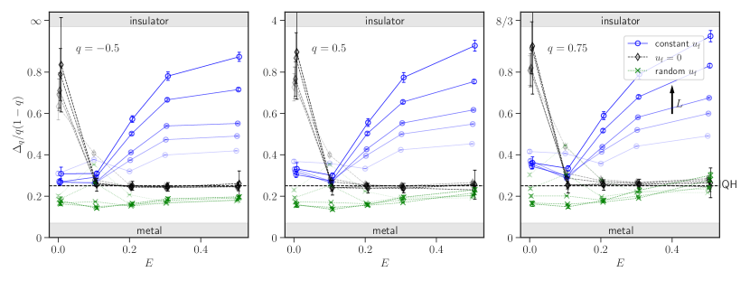
Figure 8: The scaled exponent, $\Delta_{q}/q(1-q)$ for $q=-0.5,0.5,0.75$ (left to right) and system sizes $N_{x}=8$ and $N_{y}=N_{z}=L=24$ to $L=128$ of the model (15). Black data: no fragmenting potential $u_{\rm f}=0$ [Eq. (26)] and disorder strength $W=0.15$; Blue data: a constant potential with $u_{\rm f}=0.3$ applied to the outermost surface layers, and disorder strength $W=0.2$; Green data: random fragmenting potential with zero average and standard deviation $u_{\rm f}=0.3$ [Eq. (35)], and disorder strength $W=0.2$. The horizontal dashed lines marks the value $0.25$ of quantum Hall criticality, and the localization limit, $\tau_{q}=0$ corresponds to $\Delta_{q}/q(1-q)\to\infty,4,8/3$ for $q=-0.5,0.5,0.75$ . (The value $\infty$ reflects the formal divergence of the IPR in the localized limit for negative $q$.)

For surfaces of large linear extension $L$ the IPRs are expected to asymptotically scale as

$$P^{E}_{q}\propto L^{-\tau^{E}_{q}},$$ (31)

with an effective dimension $\tau^{E}_{q}$ Evers and Mirlin (2008). Multifractality manifests itself in the appearance of a non-trivial anomalous dimension

$$\Delta_{q}^{E}=\tau_{q}^{E}-d(q-1),$$ (32)

measuring deviations from the naive dimension $d(q-1)$ expected for uniformly distributed states. The opposite extreme is that of localized states, for which $\tau_{q}=0$, reflecting the absence of scaling in system size. Presently, we are discussing a system with two distinct realizations of critical points. The first is the mirror symmetric point, $E=0$, marking the position of a topologically protected critical state. In the vicinity of this point, the system is expected to show multifractality with the anomalous dimensions Ludwig et al. (1994); Evers and Mirlin (2008),

$$\Delta_{q}^{\text{AIII}}=\Theta^{\mathrm{AIII}}q(1-q),$$ (33)

where $\Theta^{\mathrm{AIII}}$ is a non-universal coefficient depending on the disorder strength. The second is the quantum criticality otherwise realized by states sitting at the center of Landau levels in quantum Hall systems. For these states, the spectrum of scaling dimensions is approximately parabolic Huckestein (1995)

$$\Delta_{q}^{\text{QH}}\simeq\Theta^{\text{QH}}q(1-q),$$ (34)

with $\Theta^{\text{QH}}\simeq 0.25$ Evers et al. (2008); Evers and Mirlin (2008); Zirnbauer (2019). In either case, the spectrum is expected to be approximately parabolic up to a threshold $|q|\simeq q_{c}=\sqrt{2/\Theta}$ Evers and Mirlin (2008); Ludwig et al. (1994); Foster et al. (2014).

Figure 8 shows the anomalous multifractal exponent $\Delta_{q}/q(1-q)$ for $q=-0.5,0.5,0.75$ (left to right) and vanishing (dashed), constant (blue) and random (green) fragmenting potential. The different curves show data obtained for increasing system sizes $N_{y}=N_{z}=L=24$ to $128$ as a function of energy, $E$ . Numerically, we calculate an effective $L$-dependent multifractal exponent, with a finite logarithmic difference between IPRs of increasing system size $L$. The details of this procedure are delegated to Appendix B. At $E=0$ we obtain $\Theta^{\text{AIII}}\approx 0.85\pm 0.2$ ($u_{\rm f}=0$), $0.32\pm 0.05$ (constant $u_{\rm f}$), and $0.18\pm 0.03$ (random $u_{\rm f}$). Here $u_{\rm f}$ determines the fragmenting potential $U_{\rm{f}}$ (26). The approximate independence of these values on the value of $q$ and $L$ indicates that we are observing the anomalous dimension (33) of the $E=0$ quantum critical point. Away from $E=0$, our results sensitively depend on the chosen model for $u_{\rm f}$:

Zero fragmenting surface potential:

For $u_{\rm f}=0$ the data quickly drops to the value Eq. (34) expected at quantum Hall criticality. This value is maintained, including for large energies inside the bulk gap. In this way we confirm the observation of spectrum-wide criticality of Ref. Sbierski et al. (2020).

Constant fragmenting surface potential:

Upon application of a constant $u_{\rm f}=0.3$, we observe a clear tendency away from criticality and towards localized behavior upon increasing the system size. We note that the perturbation of strength $u_{\rm f}=0.3$, presently applied to only one surface layer, is by a factor of two below the threshold $u_{\rm f}^{\rm c}\simeq 0.6$ required to induce an indirect gap below surface and bulk band, see Fig. 5(c). (We restrict our attention to $|u_{\rm f}|<u_{\rm f}^{\rm c}$, because larger values require stronger disorder to observe effects in finite size.) This finding is consistent with the expectation that fragility of the surface-bulk connection — and consequently eigenstate localization at large length scales — will be induced by any constant non-vanishing $u_{\rm f}$.

Random fragmenting surface potential:

Motivated by the scenario laid out at the end of Sec. IV.4, we consider a spatially varying surface deformation $u_{\rm f}(x,y,z)$ of unit layer depth, vanishing average, and variance

$$\langle u_{\rm f}(x,y,z)\,u_{\rm f}(x,y^{\prime},z^{\prime})\rangle_{y,z}=u_{\rm f}^{2}\,\delta_{y,y^{\prime}}\,\delta_{z,z^{\prime}}$$ (35)

for $x=0$ and $x=N_{x}$. The green data shows that this perturbation leads to delocalized and quantum Hall critical behavior at finite energies, much as that of the unperturbed model. However, the convergence towards the quantum-Hall exponent is slower than in the absence of a fragmenting potential. For further discussion of this point we refer to Appendix B.2.

We conclude from the three sets of data (black, blue, green) presented in Fig. 8 that an arbitrary perturbation of the surfaces is not necessarily sufficient to localize the finite-energy states. Instead, a deformation that induces a nonzero average surface Berry curvature [e.g., $\langle u_{\rm f}(x,y,z)\rangle_{y,z}\neq 0$] is needed. This conclusion is consistent with the considerations of Sec. IV.3, where it was argued that a uniform perturbation of the form in Eq. (26) induces Berry curvature.

As discussed in Sec. IV.4, spatial fluctuations of the fragmenting potential with zero average, on the other hand, lead to a percolating network of chiral domain-wall modes. This percolating network appears at all nonzero surface-state energies as quantum-Hall criticality.

Localization was not observed in previous continuum studies Ghorashi et al. (2018); Sbierski et al. (2020); Karcher and Foster (2021) that employed a 2D minimal Dirac description, as this carries exactly zero Berry curvature as long as chiral symmetry is preserved. The fragmenting potential projects to zero in the minimal Dirac approximation. Although we consider a phase with only a single surface Dirac cone (2 surface bands), the Berry curvature necessary to localize the surface states appears in the full 4-component description of the surface-state wave functions, when the fragmenting potential is applied to the lattice Hamiltonian in Eq. (17). Alternatively, localization should occur in the continuum Dirac description when the latter is wedded to a trivial band in such a way so as to induce surface Berry curvature, see Sec. III.3. In both cases, it is essential to retain additional degrees of freedom beyond the minimal Dirac description in order to decide the fate of the surface states in the presence of disorder.

V.2 Implications for experiment

Interpreted as a topological insulator with sublattice symmetry, the model in Eqs. (15) and (17) is rather artificial. Although clean systems with approximate sublattice chiral symmetry appear in nature (e.g., graphene), simple onsite impurity potentials destroy the symmetry and revert the system to a Wigner-Dyson class. For this reason, topological phases in classes CI, AIII, and DIII have received far less attention than the quantum-Hall and quantum-spin Hall insulators.

However, the non-Wigner-Dyson classes admit natural interpretations as 3D topological superconductors Schnyder et al. (2008). Then a lattice model as in Eq. (17) can be viewed as the Bogoliubov-de Gennes quasiparticle Hamiltonian in static mean field theory Ryu et al. (2010); Foster et al. (2014); indeed Eq. (17) can be interpreted as a lattice regularization of the topological superfluid ³He-$B$ Note (4). Although quantum fluctuations are inevitable in a non-$s$-wave topological superconductor, the notion of topology is expected to carry through to fully interacting phases of matter Chiu et al. (2016).

Three-dimensional topological superconductors are protected by physical time-reversal symmetry (which transmutes into the chiral $\mathcal{S}$ condition in Eq. (IV.1) within the Bogoliubov-de Gennes language Schnyder et al. (2008)), and varying degrees of spin SU(2) symmetry. Class CI, AIII, and DI superconductors respectively possess SU(2), U(1), and no spin rotational symmetry. Beyond time-reversal and spin symmetries, no other restrictions are placed upon lattice structure or disorder realizations; see Appendix C for the explicit mapping in class AIII. This means that generic non-magnetic impurities do not alter the symmetry class for these superconductors.

The surface fluid of a bulk topological superconductor consists of unpaired fermion quasiparticles (“Dirac fermions” for classes CI and AIII, “Majorana fermions” for class DIII). This fluid can dominate certain observables at low temperature $T$. In particular, a clean surface-Dirac cone gives a power-law-in-$T$ contribution to the Meissner effect, due to the paramagnetic current of the surface Wu et al. (2020). The surface quasiparticles also contribute to the longitudinal thermal and (for classes CI and AIII) spin conductivities. By contrast, the contribution of the fully gapped bulk is exponentially suppressed for these quantities in the $T\ll\Delta_{0}$ limit, where $\Delta_{0}$ is the bulk superconducting gap.

Disorder is inevitable in real materials, and particularly at crystal boundaries. Then, the alternative scenarios of spectrum-wide criticality versus surface Anderson localization produce very different phenomenologies. Localization suppresses surface conduction, which can then be mediated at finite temperature only through inelastic processes. This should suppress the surface contribution to the Meissner effect. Without inelastic scattering, the finite-$T$ surface thermal conductivity vanishes with surface localization in the thermodynamic limit; this is because the single delocalized state at zero energy is a set of measure zero in the surface spectrum. In reality, dephasing stabilizes a surface contribution at finite $T$, analogous to the longitudinal conductivity measured at the plateau transition of the quantum Hall effect Wang et al. (2000). By contrast, spectrum-wide quantum criticality should yield a universal surface thermal conductivity determined (via the Wiedemann-Franz relation) by the average zero-temperature electrical conductivity of the quantum Hall plateau transition Sbierski et al. (2020).

Which scenario is expected to be realized experimentally? A main message of this paper is that microscopics are necessary to determine the presence or absence of average surface Berry curvature; the latter is responsible for surface localization with disorder. We note that for the cubic lattice model in Eq. (15), the fragmenting surface potential in Eq. (26) used to induce the localization in Fig. 8 breaks the average cubic rotational symmetry. Equivalently, different surface perturbations are needed to induce average surface Berry curvature on different surfaces. This suggests that point-group symmetry-breaking perturbations tailored to particular crystal terminations may be necessary to induce surface localization. Alternatively, as described in Sec. III.3, surface localization for $E\neq 0$ can be induced by coupling the surface of the AIII superconductor to a non-magnetic atomic-limit insulator. Hybridization between the insulator states and the superconductor, which is most effective if the band edge of the insulator is close to the Fermi energy of the superconductor, then yields the required Berry curvature. On the other hand, magnetic impurities or a weak external field should be sufficient to localize even the zero-energy surface state because they break the (physical) time-reversal symmetry protecting the class-AIII superconductor. This would exponentially suppress the longitudinal surface thermal conductivity at low temperatures.

VI Field theory

In this section, we discuss how the physics discussed above presents itself from the perspective of effective field theory. It is self contained, and included to provide an analytical justification for the criterion of state delocalization used empirically in previous sections. Readers willing to accept the evidence provided so far as convincing enough may consider this section as optional or skip it.

By “field theory,” we here mean theoretical frameworks in which averaging over static disorder is performed at an early stage to describe $d$-dimensional systems in a given symmetry class in terms of $(d+0)$ dimensional  nonlinear $\sigma$-models. Such theories have been in use for a long time in the physics of conventional disordered metals (see the textbook Efetov (1997) for review) and were extended to the description of various topological insulators Gruzberg et al. (1999, 2001); Altland and Merkt (2001) even before the momentum space topologies of clean insulators became understood. In parallel to that developement, the approach was upgraded to a full classification of disordered topological insulators Ryu et al. (2010) alternative to, say, the mathematical framework of non-commutative geometry Schulz-Baldes (2016). From an applied perspective, its strength is that it can predict, e.g, the flow of transport coefficients Pruisken (1984); Altland et al. (2015); Fu and Kane (2012) as a function of disorder strength or system size. It is this latter aspect that will be important in our discussion below.

We begin with a short review of the physics of the two-dimensional class A, and the three-dimensional AIII insulator, extending the discussion of Sec. II.2 to the presence of disorder. While these are known structures, included here to provide perspective, our discussion of the AIII surface in section VI.3, and specifically that of a connection between field theoretical topological $\theta$-angles and momentum space Berry curvature in Appendix A is new material.

VI.1 Two-dimensional Chern insulator

The starting point of field theoretical representations of topological insulators is an intermediate action (see Appendix A for a brief review of its derivation) of the form

$$S[X]\equiv-\tr\ln{(E-\hat{H}(\textbf{k})+i\kappa\hat{X}(\textbf{x}))},$$ (36)

where k and x are momentum and position, respectively, $\hat{H}(\textbf{k})$ is the clean Hamiltonian (throughout, we will omit carets on operators in their eigenbasis representation), $\kappa$ a parameter measuring the effective disorder scattering rate, and $\hat{X}=\{X^{rr^{\prime}}_{ss^{\prime}}\}$ a matrix valued slowly fluctuating field carrying a replica index $r=1,\dots,R$ (sometimes traded for the mathematically more rigorous internal supersymmetry structure Efetov (1997)), and a second index $s=\pm=\pm 1$ distinguishing between propagators of retarded and advanced causality. Further details of the internal structure of $\hat{X}$ depend on the symmetry class under consideration. For example, in class A, $\hat{X}\equiv Q=T\hat{\tau}_{3}T^{-1}$, where $\hat{\tau}_{3}$ will be a Pauli matrix in $s$-space throughout this section (not to be confused with the earlier sublattice/chiral ${\tau}_{3}$) or in AIII just $Q=T$.

The further processing of the action reflects a notion of real and momentum space duality, according to which the momentum space symmetries and topology encoded in $H(\textbf{k})$ determine the real space symmetries and topology of $Q(\textbf{x})$. To demonstrate the principle, consider the first step towards a gradient expansion in class A and use the unitary invariance of the trace to transform the action to

$$S[Q]\equiv-\tr\ln\left(\hat{G}^{-1}(E,\textbf{k})-[T^{-1}(\textbf{x}),\hat{H}(\textbf{k})]T(\textbf{x})\right).$$ (37)

Here, we encounter the impurity broadened Green function of the system $\hat{G}^{-1}(\textbf{k})\equiv E-\hat{H}(\textbf{k})+i\kappa\hat{\tau}_{3}$ in conjunction with a term in which the real- and momentum-space dependent terms of the action talk to each other. Assuming smooth variation of its two constituents, a first order Wigner-Moyal expansion leads to $[T^{-1}(\textbf{x}),\hat{H}(\textbf{k})]T(\textbf{x})\approx F_{i}(\textbf{k})\Phi_{i}(\textbf{x})$, with $F_{i}=i\partial_{i}\hat{H}$ and $\Phi_{i}\equiv(\partial_{i}T^{-1})T$, where the derivatives are with respect to $k_{i}$ and $x_{i}$, respectively. The effective action describing the system at large distance scales then is obtained by expansion of the tr ln up to second order in the derivative terms $\Phi_{i}$. Notice that the real space $\Phi_{i}$ always appear in conjunction with momentum space $F_{i}$. Also note that to leading order in a derivative expansion,

$$\tr(\hat{A}(\mathbf{x})\hat{B}(\mathbf{k}))=\int dxdk\,\tr(\hat{A}(\mathbf{x})\hat{B}(\mathbf{k}))$$ (38)

where $dx=d^{d}x$ and $dk=d^{d}k/(2\pi)^{d}$, and the trace on the right hand side is over the internal matrix structure of the operators in question. In this way, terms appearing in the action naturally assume the form of (momentum space integrals) $\times$ (real space integrals), where in the case of topological terms, the two partners encode “dual” aspects of the topology of the system.

Specifically, for the case of the two-dimensional Chern insulator, the result of the expansion to second order in gradients is Pruisken’s nonlinear $\sigma$-model, which first appeared in the context of the integer quantum Hall effect Pruisken (1984),

$$S[Q]=g\int d^{2}x\,\tr(\partial_{i}Q\partial_{i}Q)+\frac{\theta\epsilon_{ij}}{16\pi}\int d^{2}x\,\tr(Q\partial_{i}Q\partial_{j}Q).$$ (39)

Here, the first term describes the diffusion and eventually Anderson localization of a two-dimensional electron gas in the presence of disorder, where the bare value of the coupling constant $g=\sigma_{xx}/8$ is set by the system’s longitudinal conductance. The second term is of topological nature and counts the number of times the $Q$-matrix field winds around its target manifold. In the classical reference its weighing topological angle $\theta=2\pi\sigma_{xy}$ was identified with the Hall conductance. Of more relevance to our present discussion is its interpretation as a momentum space dual of the real space term, namely $\theta=\theta(E)$ as given in Eq. (27). (This expression is derived for general two-dimensional systems in class A in Appendix A.)

As derived, the action Eq. (39) describes the system at “bare length scales,” with a minimal distance cutoff set by the scattering mean free path. Upon integrating out short distance fluctuations, and for generic values of $E$, the coupling constant $g$ renormalizes to zero (Anderson localization), while the effective angle $\theta$ renormalizes to a multiple of $2\pi$ (Hall quantization). For these fixed point values, the topological $\theta$-action reduces to a boundary action $\frac{1}{8}\epsilon_{ij}\int d^{2}x\,\tr(Q\partial_{i}Q\partial_{j}Q)=S_{\textrm{1d}}[T]$, where

$$S_{\mathrm{1d}}[T]\equiv\frac{1}{2}\oint dx\,\tr(T^{-1}\hat{\tau}_{3}\partial_{x}T),$$ (40)

and $x$ now is a one-dimensional boundary coordinate. This single derivative action describes the dissipationless chiral circulation of boundary currents against the protecting background of a localized bulk. As with the chiral Hamiltonian of the clean system it lacks gauge invariance, signalling spectral flow through the delocalized states at the energies $E_{+}$ or $E_{-}$.

We next compare this physics to that in our reference system without protected spectral flow.

VI.2 Three-dimensional AIII insulator

As with its lower-dimensional cousin, the gradient expansion of the prototypical action (36) leads to a nonlinear $\sigma$-model Gade and Wegner (1991); Altland and Simons (1999) enriched by a topological term Ryu et al. (2010),

$$S_{\textrm{3d}}[T] =\int d^{3}x\,\bigg{[}g\,\tr(\partial_{i}T\partial_{i}T^{-1})+E\nu\tr(T+T^{-1})\bigg{]}+$$ (41)

$$+\frac{\vartheta\epsilon^{ijk}}{24\pi^{2}}\int d^{3}x\,\tr(T^{-1}\partial_{i}TT^{-1}\partial_{j}TT^{-1}\partial_{k}T).$$ (42)

Compared to Eq. (39), the field manifold has changed to group-valued matrix fields, $T\in\mathrm{U}(2R)$. Otherwise, we again have a job division between a gradient term describing bulk conduction properties, and a topological term now measuring three-dimensional windings over the unitary group. The second term describes the symmetry breaking induced by departures away from $E=0$, where $\nu$ is proportional to the three-dimensional density of states.

There are different physical limits that may be investigated on the basis of this representation: at the particle-hole symmetric point $E=0$ we are sitting inside the bulk spectral gap. The bare conduction parameter $g$ may nevertheless be finite, due to impurity states smearing the band gap of the clean system. At large length scales, we expect renormalization to an Anderson insulator, $g=0$, where a value $\vartheta=2\pi n$ with $n$ a non-vanishing integer will signal topological non-triviality. In this limit, and in analogy to the Pruisken action, the topological term becomes a boundary term, $\Gamma[T]/12\pi$, with the physical interpretation of a Wess-Zumino term Altland et al. (2002) of an emerging surface action. In the immediate vicinity of the surface, the gradient term remains finite and now describes intra-surface conduction. The net effect is the stabilization of a surface Wess-Zumino action

$$S_{\textrm{2d}}[T] =g\int d^{2}x\,\tr(\partial_{i}T\partial_{i}T^{-1})+\frac{1}{12\pi}\Gamma[T],$$ (43)

through the localization of the bulk. This action is the AIII analog of Eq. (40) for the A system. At large length scales, this theory renormalizes Nersesyan et al. (1994); Altland et al. (2002) to the conformally invariant action with $g=1/8\pi$ representing a single two-dimensional Dirac point at zero energy; this is the field theoretical interpretation of zero energy surface delocalization in the AIII insulator.

However, we may also investigate what happens at finite deviations $E\not=0$ away from chiral symmetry. In this case, the (strongly RG relevant) “mass term” in Eq. (41) only admits configurations $T\to Q=T\hat{\tau}_{3}T^{-1}$ for which $\tr(Q+Q^{-1})$ is a constant vanishing in the replica limit. These are the $Q$-matrices of the model of lower symmetry AIII $\to$ A. Substitution into the bulk action annihilates the second and third term, while the gradient term becomes the conventional action of a disordered three-dimensional metal below the Anderson transition point: away from zero energy, the AIII insulator behaves like a conventional Anderson insulator. A more interesting limit is the case of small but finite $E\not=0$ in the vicinity of the surface. The symmetry breaking now collapses the Wess-Zumino term $\Gamma[Q]$ to the Pruisken term of a two-dimensional class A action, at topological angle $\theta=(2\mathbb{Z}+1)\pi$ Altland et al. (2002). We conclude that the naive extension of the zero-energy WZW action to finite energies equals the action Eq. (39) of a two-dimensional Chern insulator fine tuned into criticality. This is a field theoretical indication of a tendency to extended surface quantum criticality. The question is what happens for larger deviations $E$ away from zero. To answer it, we need to go beyond the present level of high level reasoning and turn to a first principle approach.

VI.3 Surface of the three-dimensional AIII insulator

In order to understand the physics of the disordered surface at arbitrary $E$, we again start from the prototypical representation (36). For the slow field, we take $\hat{X}(\mathbf{x})=(T\hat{\tau}_{3}T^{-1})(\mathbf{x})$, where $\mathbf{x}$ is a two-dimensional surface coordinate. (The justification behind this surface projection is that states of finite extension into the bulk have eigenenergies much larger than $E$, which we assume to be way below the bulk gap.) For the surface Hamiltonian $\hat{H}(\mathbf{k})$, we assume a spectral decomposition

$$\hat{H}(\mathbf{k})\equiv\sum_{\alpha}|\alpha_{\textbf{k}}\rangle\,\epsilon_{\alpha_{\mathbf{k}}}\langle\alpha_{\mathbf{k}}|,$$ (44)

where $\{|\alpha_{\textbf{k}}\rangle\}$ are the system eigenstates at a given transverse momentum.

This formal spectral decomposition actually is less innocent than it looks: Naively, it should include all eigenstates at a given $\mathbf{k}$. However, this is not the case. Going back to the tr ln (36), only eigenstates of $\hat{H}(\textbf{k})$ with a finite spatial overlap with the surface Hubbard-Stratonovich field $\hat{X}(\textbf{x})$ contribute to the expansion. The obvious candidates here are the two eigenstates forming the chiral partners of the surface band. However, the internal spinor representation space at a given k of the lattice model is four-dimensional, implying that two states are insufficient to span it. We must, therefore, assume a contribution of bulk states (with finite surface amplitude), and an associated state-dependent weight $\kappa=\kappa_{\alpha}$. As we do not have full access to this information, we sidestep the problem by considering Eq. (44) as a formal complete sum. We also consider the surface band for the flattened model, i.e. we assume a finite spectral gap to higher-lying bands.

In Appendix A we show that under these conditions, the surface action assumes the form of a two-dimensional class A action Eq. (39), with the topological angle given by Eq. (27), or Eq. (46) in a more explicit representation. As discussed above, the added curvature integrals of the upper and lower surface band computed in this way need not add to zero. In view of the above discussion, this phenomenon relates back to the embedding of the surface band into a larger Hilbert space of bulk states. Unlike with intrinsic two-dimensional lattice bands, whose Chern numbers would have to add to zero, we are here considering a single two-dimensional shadow of a three-dimensional bulk (the other lives at the opposite surface) and the cancellation principle does not apply.

VII Discussion and conclusion

For topological insulators in the Wigner-Dyson classes A, AI, and AII — the most prominent realizations being the two-dimensional class A integer quantum Hall insulator and class AII quantum spin Hall insulator, and the three-dimensional class AII topological insulator — boundary states are continuously attached to delocalized bulk states, without interruption by a spectral or mobility gap. In this paper, we showed that for the complementary class of “genuinely” non-Wigner-Dyson class topologlogical insulators this key principle is broken. (The attribute “genuine” indicates that the constraints imposed by charge conjugation symmetry ${\cal C}$ or chiral symmetry ${\cal S}$ that define the non-Wigner-Dysnon classes and force the spectrum to be symmetric around $E=0$ are essential for the protection of the bulk topology. By contrast, “non-genuine” classes remain topological after lifting constraints due to ${\cal C}$ and ${\cal S}$ behave effectively as Wigner-Dyson insulators.)

In the literature, nontrivial topology is often associated with an obstruction to the construction of a localized basis of conduction and valence bands, referred to as “Wannierizability”. Our general results — see Tab. 1 — show that, by contrast, all genuine non-Wigner-Dyson class insulators enjoy this property, and can be topologically non-trivial nonetheless. We arrived at these conclusions both from a bulk perspective, showing that localizability of the bulk implies that the connection between surface and bulk bands becomes fragile, and from an intrinsic boundary perspective, showing that the effective surface theory admits a gap-opening perturbation. A key conclusion following from this observation is that the surface states of genuine non-Wigner-Dyson topological insulators themselves are localizable, except at the center $E=0$ where state delocalization is topologically protected.

The existence of gapless or conducting surfaces is the key signature distinguishing topological from conventional insulators. Our analysis shows that, in this regard, the physics of genuine non-Wigner-Dyson topological insulators is different from that of their Wigner-Dyson siblings: Their surface states can, but need not be delocalized away from one isolated energy, $E=0$. As a concrete case study, we considered the three-dimensional AIII insulator and showed that the spectrum of different scenarios ranges from full delocalization of all states in a surface band connected to a bulk band, to localization of all states away from zero energy. The situation is “fragile” in that the tuning of local lattice potentials may continuously interpolate between these extremes. Depending on which option is realized, one expects different behavior of surface thermodynamic and transport properties, as discussed in section V.2.

Indeed, our study was motivated by recent work, which reported a spectrum-wide delocalization of the surface states of a class-AIII insulator and other non-Wigner-Dyson classes Ghorashi et al. (2018); Sbierski et al. (2020); Ghorashi et al. (2020); Karcher and Foster (2021). These observations were based both on a numerical analysis of an effective Dirac surface theory and a numerical study of a three-dimensional lattice model of a class-AIII insulator. In this work we identified the principles that led to this seemingly robust prediction. We showed that the minimal $2\times 2$ Dirac theory considered in these references is intrinsically protected against localization. However this protecition is topologically fragile in that it is lifted if additional trivial surface bands are added (which can be achieved, e.g., by coupling an extraneous surface layer). The absence of localization in the full three-dimensional lattice model considered in Ref. Sbierski et al. (2020) results from a statistical symmetry, similar to that realized in the “statistical topological insulator” Fulga et al. (2014).

For the case of minimal topological winding number $\nu=1$, we identified a powerful indicator for the localization properties of states at energy $E$, namely the integrated Berry curvature of all states energetically below (or equivalently above) that energy: an integer-quantized integral implies delocalization, departures from these values localization. While the energetic non-locality of this criterion may be unexpected for a model of non-interacting particles, it reflects the importance of global momentum space quantum geometry in a topologically nontrivial context. In the two models mentioned above, that criterion signals global delocalization, if for different reasons: the minimal surface Dirac theory is Berry-flat; in the lattice model, the disorder model considered in Ref. Sbierski et al. (2020) leads to a statistical cancellation of curvature in the integral. However, both the embedding of the minimal $2\times 2$ theory into a four-component spinor theory (the minimal framework to describe topological non-triviality in three-dimensional AIII), or the lifting of the statistical symmetry in the lattice model by addition of a “fragmenting surface potential” of non-zero average, lead to state localization in a manner discussed in detail in section V.

At the same time, our analysis indicates that for winding numbers $|\nu|>1$, the precise meaning of the term “minimal model”, and the identification of quantitative localization measures must be reconsidered. In conclusion, the principle that a localizable bulk implies a gapable surface spectrum (and vice versa) applies to all “genuine” non-Wigner-Dyson classes. Other observations, such as the precise ways in which the minimal Dirac description is fragile, and the relation of localizability and Berry curvature, need not straightforwardly generalize beyond the $\nu=1$ AIII context and invite future work.

Most of the previous work on surface state localization in the AIII insulator considered a low-energy, continuum two-dimensional Dirac description with two-component Dirac spinors Bernard and LeClair (2002); Foster et al. (2014). Our results imply that these theories are fundamentally incomplete, because the surface Berry curvature responsible for Anderson localization is strictly ruled out. To readers who trust in the predictive power of minimal models, it is a surprising and possibly disturbing notion that such Lorentz-covariant and renormalizable field theories cannot encode the most basic characteristics (localized versus extended) of surface-state wave functions. At the same time, it may be reassuring that the origin of the problem does not lie in the notorious and difficult-to-handle lack of ultraviolet closure of the Dirac theories, but that the problem can be cured by the simple addition of trivial degrees of freedom. Allowing for the addition of trivial bands is common practice in topological classifications based on stable equivalence, and our results show that it is equally important when determining the existence of a topological obstruction to Anderson localization.

Acknowledgements:

We thank Jennifer Cano, Sayed Ali Akbar Ghorashi, Alex Kamenev, Bastien Lapierre, Herrmann Schulz-Baldes, Haruki Watanabe, and Justin Wilson for helpful discussions. This work was supported by the Deutsche Forschungsgemeinschaft (DFG) project grant 277101999 within the CRC network TR 183 (subproject A03) (A.A., P.W.B., M.M.-G.), the German Academic Scholarship Foundation and the German Research and the Collaborative Research Center SFB 1277 (J.D.), the Welch Foundation Grant No. C-1809 (M.S.F.), and by the FNS/SNF Ambizione Grant No. PZ00P2_179962 (L.T.).

Appendix A Field theory analysis

In this section we discuss the field theoretical analysis of the disordered surface. To make the paper self-contained, we start with a quick review of the derivation of the intermediate representation Eq. (36), here formulated for class A for concreteness. In a second step we then show that the expansion of that action establishes a connection between the $\theta$-term describing the real space surface topology in the presence of disorder and the integrated momentum space Berry curvature.

A.1 Replica field theory

We begin by adding disorder a potential $\hat{V}(\textbf{x})$ with variance $\langle\hat{V}(\textbf{x})\hat{V}(\textbf{x}^{\prime})\rangle=\frac{\gamma_{0}}{2}\delta(\textbf{x}-\textbf{x}^{\prime})$ to the clean Hamiltonian $\hat{H}$ . Transport observables such as the longitudinal or transverse conductance at characteristic energy $E$ may be computed from the $R$-fold replicated partition sum Wegner (1979)

$$Z^{R} =\int D\psi\exp(-S[\psi]),$$

$$S[\psi] =-i\int dV\,\bar{\psi}(E+i\delta\hat{\tau}_{3}-\hat{H}-\hat{V})\psi,$$

where $\psi=\{\psi_{s,\mu}^{r}(\mathbf{x})\}$ is a Grassmann field, the index $\mu=1,\dots,4$ labels the components of the lattice spinor, $r=1,\dots,R$ is a replica index, $s=1,2$ distinguishes between advanced and retarded components, and $\hat{\tau}_{3}$ is a Pauli matrix in advanced/retarded space. We average the partition sum over disorder to obtain a quartic interaction potential between replicas,

$$S[\psi] =S_{0}[\psi]+\frac{\gamma_{0}}{2}\int dV(\bar{\psi}\psi)^{2},$$ (45)

where $S_{0}$ is the clean action. To decouple the quartic term, we introduce a Hubbard-Stratonovich matrix field $B(\textbf{x})=\{B_{ss^{\prime},ii^{\prime}}^{rr^{\prime}}(\textbf{x})\}$. Integrating out the $\psi$ fields yields,

$$\left<Z^{R}\right> =\int DB\exp\left(-\frac{1}{2\gamma_{0}}\int dV\tr B^{2}+\tr\ln\hat{G}[B]\right),$$

with $\hat{G}[B]=(E+i\delta\hat{\tau}_{3}-\hat{H}-B)^{-1}$. A variation of the action in $B$ leads to $\bar{B}(\textbf{x})=\gamma_{0}\tr\hat{G}[\bar{B}](\textbf{x},\textbf{x})$, which has the structure of a self-consistent Born equation. According to it, the mean field $\bar{B}$ pays the role of an impurity scattering “self energy” whose strength is determined by the impurity-broadened local spectral density, $\hat{G}[\bar{B}](\textbf{x},\textbf{x})$. The equation is solved by the diagonal ansatz $\bar{B}=-i\kappa\hat{\tau}_{3}$, where $\kappa$ an effective scattering rate determined by the bare strength $\gamma_{0}$. For our purposes, we need not discuss the self-consistent dependence $\kappa(\gamma_{0})$ in detail. However, what does matter is that the stationarity equation affords a whole manifold of solutions besides the matrix-diagonal one, $B=-i\kappa T\hat{\tau}_{3}T^{-1}=-i\kappa Q$, where $T\in U(2R)/(U(R)\times U(R))$, and $Q=T\hat{\tau}_{3}T^{-1}$. Physically, these are the Goldstone modes associated to the “spontaneous symmetry breaking” $i\delta\to i\kappa$ reflected in the upgrade of the infinitesimal causal parameter $i\delta$ to the finite damping $i\kappa$.

Substituting these modes into the action, and noting that $\tr(Q^{2})=\textrm{const}.$ is a constant (vanishing in the replica limit), we arrive at the soft mode action (36) which will be our starting point for all further considerations.

A.2 Gradient expansion

We now discuss the steps required to advance from Eq. (36) and its equivalent representation (37) to a local action containing of lowest non-vanishing order in gradient operators. There are only two of these consistent with the symmetries of the model, namely $\tr(\partial_{i}Q\partial_{i}Q)$ and $\epsilon_{ij}\,\tr(Q\partial_{i}Q\partial_{j}Q)$. The derivation of an action containing the first via expansion of the tr ln is textbook material Efetov (1997) (see also Ref. Moreno-Gonzalez et al. (2023) for the specific case of the two-dimensional topological class A insulator) and is not of primary relevance to our present discussion. However, the construction of a topological action containing the second terms is concerned, we need to start afresh; previous derivations of this action where specific to the quantum Hall effect Pruisken (1984), or other genuinely two-dimensional materials Ostrovsky et al. (2007). By contrast, we here want to allow for situations where the effective $H(\mathbf{k})$ is given by a general spectral decomposition as in Eq. (44). In this way, we will address all class A situations relevant to our discussion (bulk two-dimensional insulators for the sake of comparison, and the AIII surface at finite energies) in one go.

The second order expansion of the tr ln in the combinations $F_{i}\Phi_{i}$ defined after Eq. (37) leads to two terms, $S\to S_{\textrm{top}}=S^{(1)}+S^{(2)}$, where $S^{(1)}=-\,\tr(\hat{G}F_{i}\Phi_{i})$, and $S^{(2)}=\frac{1}{2}\,\tr(\hat{G}F_{i}\Phi_{i})^{2}$, and the subscript “top” indicates that we wish to isolate the topological contribution to the action. Naively, one might think that the first order term drops out by symmetry. However, this is not so because the trace over a single Green function leads to ultraviolet divergent expressions, i.e. we are facing a $0\times\infty$ situation. The way out, originally suggested by Pruisken, is to process the first order term as

$$S^{(1)} =-\int_{E}^{\infty}d\epsilon\tr(\hat{G}F_{i}\Phi_{i}\hat{G})\approx-\frac{i}{2}\int dxdk\int_{E}^{\infty}d\epsilon\,\tr((\partial_{j}\hat{G})F_{i}(\partial_{j}\Phi_{i})\hat{G}-\hat{G}F_{i}(\partial_{j}\Phi_{i})\partial_{j}\hat{G})=$$

$$=-\frac{i}{4}\int_{E}^{\infty}d\epsilon\int dk\sum_{s}s\,\tr([\hat{G}^{s},\partial_{j}\hat{G}^{s}]F_{i})\int dx\,\tr(\hat{\tau}_{3}\partial_{j}\Phi_{i}),$$

where in the first equality we used $\hat{G}(E)=-\int_{E}^{\infty}d\epsilon\,\hat{G}^{2}(\epsilon)$ to increase the number of Green functions, thereby mitigating the UV issues. To keep the notation slim, we omit the energy arguments throughout. In the second equality we applied another Moyal expansion (with $\partial_{i}\hat{G}=\partial_{k_{i}}\hat{G}(\mathbf{k})$), and used that only the imaginary part $F(\hat{G})\to\frac{1}{2}(F(\hat{G}^{+})-F(\hat{G}^{-}))\hat{\tau}_{3}=\frac{1}{2}\sum_{s}sF(\hat{G}^{s})\hat{\tau}_{3}$ will contribute to a non-vanishing trace. With the second of the two auxiliary identities

$$-4\epsilon_{lm}\sum_{s}\,\mathrm{tr}(sP^{s}\Phi_{l}P^{-s}\Phi_{m})=4\epsilon_{lm}\mathrm{tr}(\hat{\tau}_{3}\partial_{l}\Phi_{m})=\epsilon_{ij}\tr(Q\partial_{i}Q\partial_{j}Q)\equiv\mathcal{L}_{\mathrm{top}}(Q),$$

we reduce this expression to $S^{(1)}=I_{1}\int dx\,\mathcal{L}_{\mathrm{top}}(Q)$, with the energy-momentum integral

$$I_{1}=\frac{i}{32}\int_{E}^{\infty}d\epsilon\int dk\sum_{s}s\epsilon_{ij}\,\tr([\hat{G}^{s},\partial_{j}\hat{G}^{s}]F_{i}).$$

Turning to second order term and using the first of the above auxiliary relations, it is straightforward to derive an analogous expression, $S^{(2)}=I_{2}\int dx\,\mathcal{L}_{\mathrm{top}}(Q)$, where

$$I_{2}=-\frac{1}{32}\epsilon_{ij}\int dk\sum_{s}s\,\tr(\hat{G}^{s}F_{i}\hat{G}^{-s}F_{j}),$$

and we again retain only contributions which combine to a non-vanishing trace. It remains to make sense of the momentum integrals, $I_{1}$ and $I_{2}$. To this end, we engage the eigenfunction representation,

$$\hat{G}(E)=\sum_{\alpha}|\alpha\rangle\frac{1}{E+is\kappa-\epsilon_{\alpha}}\langle\alpha|,\qquad F_{i}=-i\partial_{i}\hat{H}=-i\sum_{\alpha}\epsilon_{\alpha}\partial_{i}|\alpha\rangle\langle\alpha|,$$

where we anticipate that momentum derivatives of energies will not contribute to an expression of topological significance (this can be checked by explicit computation). Substituting the first of these identities into $I_{1}$, the energy dependent denominators can all be pulled out and integrated over. As a result, we obtain

$$I_{1}=\frac{i\pi}{16}\int dk\epsilon_{ij}\sum_{\alpha\beta}\frac{1}{\epsilon_{\alpha}-\epsilon_{\beta}}\left(\delta(E-\epsilon_{\alpha})+\delta(E-E_{\beta})-\frac{2}{\epsilon_{\alpha}-\epsilon_{\beta}}\left(\Theta(\epsilon_{\alpha}-E)-\Theta(\epsilon_{\beta}-E)\right)\right)\langle\alpha|\partial_{j}\hat{H}|\beta\rangle\langle\beta|\partial_{i}\hat{H}|\alpha\rangle,$$

where we assumed the disorder to be weak enough to justify the approximation $\delta(E-\epsilon_{\alpha})=-\frac{1}{\pi}\mathrm{Im}(E+i\kappa-\epsilon_{\alpha})^{-1}$. In $I_{2}$ no energy integral needs to be done, and the substitution of the spectral decomposition leads to

$$I_{2}=-\frac{i\pi}{16}\epsilon_{ij}\sum_{\alpha\beta}\int(dk)\frac{1}{\epsilon_{\alpha}-\epsilon_{\beta}}\left(\delta(E-\epsilon_{\alpha})+\delta(E-\epsilon_{\beta})\right)\langle\alpha|\partial_{i}\hat{H}|\beta\rangle\langle\beta|\partial_{j}\hat{H}|\alpha\rangle.$$

We observe that in the combination $S_{\textrm{top}}=(I_{1}+I_{2})\int dx\,\mathcal{L}_{\textrm{top}}(Q)$ the on–Fermi–shell term $I_{2}$ cancels against the on–shell contributions of $I_{1}$, a phenomenon which in the context of the quantum Hall effect is known as the cancellation of the Streda I Fermi surface conductance against a contribution to the Streda II conductance Pruisken (1984). In a final step, we substitute the second of the above spectral decompositions to compute the matrix elements as $\langle\alpha|\partial_{i}\hat{H}|\beta\rangle=\epsilon_{\beta}\langle\alpha|\partial_{i}\beta\rangle+\epsilon_{\alpha}\langle\partial_{i}\alpha|\beta\rangle=(\epsilon_{\alpha}-\epsilon_{\beta})\langle\partial_{i}\alpha|\beta\rangle$. Substitution into $I_{1}+I_{2}$ leads to the final result

$$S_{\textrm{top}}[Q]=\frac{1}{16\pi}\int d^{2}k\,\Omega_{k}\Theta(\epsilon_{\alpha}-E)\,\int dx\,\epsilon_{ij}\tr(Q\partial_{i}Q\partial_{j}Q),$$ (46)

where $\Omega_{k}=i\langle d\alpha|\wedge d\alpha\rangle=i\epsilon_{ij}\langle\partial_{i}\alpha|\partial_{j}\alpha\rangle$.

Appendix B Details of numerical calculation of the multifractal spectra

B.1 Effective multifractal exponent

In practice to analyze the convergence of the numerical calculation in the linear surface dimension $L$ we define an effective $L$-dependent multifractal dimension

$$\tau_{q}^{E}(L)=-\frac{\ln P_{q}^{E}(L)-\ln P_{q}^{E}(L/2)}{\ln L-\ln L/2}.$$ (47)

For a critical point with multifractal scaling, this quantity will converge to the true multifractal exponent $\lim_{L\to\infty}\tau_{q}^{E}(L)\to\tau_{q}^{E}$ according to Eq. (31). Evers and Mirlin (2008) However, away from a critical point, where wave functions localize for sufficiently large system sizes, $L$, its value will not converge until $L$ is larger than the localization length and $\tau_{q}^{E}\to 0$. In this way the effective exponent allows us to distinguish between a localizing and critical behavior. In the latter case, it also quantifies the convergence of the multifractal spectrum.

B.2 Distribution functions of inverse participation ratios

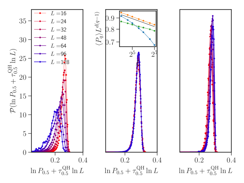
Figure 9: Distribution functions of $P_{q}$ at $q=0.5$ for $u_{\mathrm{f}}=0.3$ (left), $u_{\mathrm{f}}=0$ (middle), and $u_{\mathrm{f}}$ random (right) with $\mathrm{rms}\,u_{\mathrm{f}}=0.5$. (Here, the topological control parameter is $M=2.0$ and the disorder strength is $W=0.2$.) The horizontal axis has been rescaled as discusseed in the text. Inset: the convergence of the mean of the IPRs, scaled by the trivial scaling exponent of fully extended states for constant (blue), zero (yellow) and random (green) $u_{\mathrm{f}}$.

In a numerical experiment, the moments $P_{q}$ are randomly distributed quantities, whose mean values are shown in Fig. 8. The probability distribution of the moments $P_{0.5}$ is shown in Fig. 9, again for the three cases constant, zero and random $u_{\rm f}$. For ideal quantum Hall criticality, we expect $P_{0.5}=c\,L^{-\tau_{0.5}}$, with the exponent [cf. Eqs. (32) and  (34)] $\tau_{0.5}\approx-1+\frac{1}{16}$. This implies that the variable $\ln[P_{0.5}+\tau_{0.5}\ln(L)]$ should be distributed around the non-universal constant $\ln c$ Evers and Mirlin (2008); Puschmann et al. (2021). The figure shows for $u_{\rm f}=0$ (center) this variable is indeed narrowly distributed around a maximum, with data collapse for all values of $L$. Qualitatively similar behavior is found for random $u_{\mathrm{f}}$ (right). While, for the numerically accessible system sizes the scaling limit is harder to reach in this case, the collapse becomes more pronounced for our largest values of $L$, shown in blue. However, for non-vanishing constant $u_{\mathrm{f}}$ (left) the data cannot be scaled to collapse, including for different values of $\tau_{0.5}$. In this way, the absence of criticality reveals itself.

In the inset we show the scaling of the mean of the moments with system size, rescaled by the trivial extended scaling behavior. Blue (yellow, green) data represents the finite (vanishing, random) $u_{\mathrm{f}}$, where the latter two asymptote towards the QH scaling indicated as a black dotted line.

B.3 Convergence in transverse direction

We here demonstrate that already small slab widths $L_{x}$ are sufficient to make quantitative statements about the localization properties of the surface states. As an example, Fig. 10 shows the distrubtion function of the moments $P_{0.5}$ for $u_{\mathrm{f}}=0$ and a surface extension $L=64$ for different values of $L_{x}$. The full distribution function, including mean and tails, coincide, indicating that for all shown slab widths the distribution function are already converged.

The reason for the observed width–independence is the exponential transverse localization of surface states, with a decay length of order one layer or less. Here, and in the numerical calculations shown above, only surface states with a surface weight of more than $75\%$ are taken into account to avoid artefacts due to low lying bulk states. (These are rare but they exist due to disorder inside the clean bulk gap.)

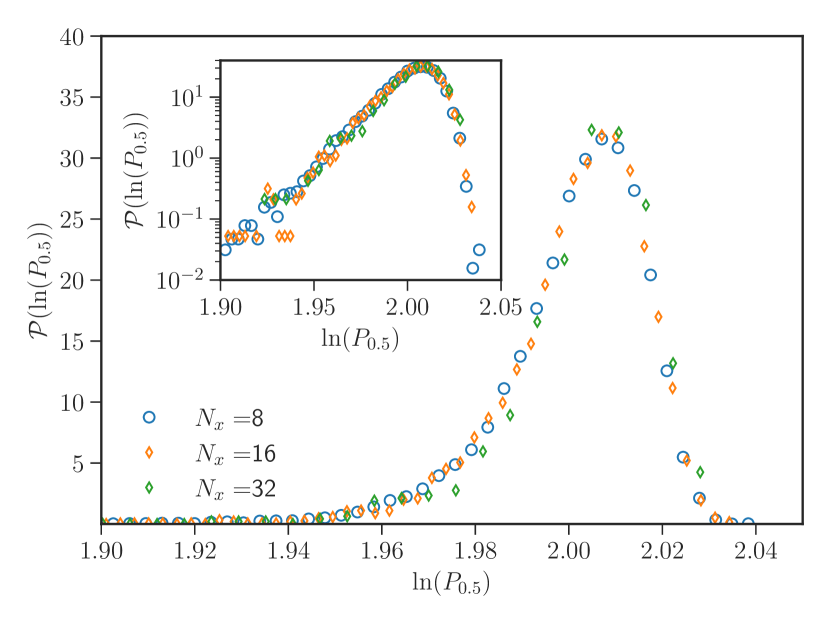
Figure 10: Distribution functions of $P_{q}$ at $E=0.1$, $u_{\mathrm{f}}=0$, $W=0.15$ and linear surface extension $L=64$ for different slab widths $N_{x}$ on a linear (main) and semi-logarithmic scale (inset).

Appendix C Class AIII superconductors

In a superconductor with a spin rotational invariance around a fixed axis, the Bogoliubov-de Gennes (BdG) Hamiltonian $H=\mbox{diag}\,(h_{\uparrow},h_{\downarrow})$ splits into two blocks, corresponding to “spin up” and “spin down” sectors. (The BdG Hamiltonian acts on four-component spinors with spin and particle-hole degrees of freedom.) Particle-hole conjugation $\mathcal{C}$ and time-reversal symmetry $\mathcal{T}$ map these two blocks onto each other,

$$h_{\uparrow}=-\mathcal{C}^{-1}h_{\downarrow}\mathcal{C}=\mathcal{T}^{-1}h_{\downarrow}\mathcal{T},$$ (48)

so that it is sufficient to consider the “spin-up” block $h\equiv h_{\uparrow}$ only. The product $\mathcal{S}=\mathcal{CT}$ acts as an antisymmetry constraint on the Hamiltonian,

$$h=-\mathcal{S}^{-1}h\mathcal{S}.$$ (49)

It follows that a superconductor with time-reversal symmetry and a remnant U(1) of spin SU(2) rotational invariance resides in class AIII Schnyder et al. (2008); Foster and Ludwig (2008). We now make these arguments more explicit, using a formulation in terms of fermion creation and annihilation operators, so that particle-hole symmetry is automatically encoded in the fermion anticommutation relations and need not be implemented explicitly.

For a system of spin-1/2 electrons, we can form the spin-triplet Cooper-pair annihilation operator in position space

$$b_{a}(\bm{\mathrm{r}},\bm{\mathrm{r^{\prime}}})\equiv \,c_{\sigma}(\bm{\mathrm{r}})\,c_{\sigma^{\prime}}(\bm{\mathrm{r^{\prime}}})\,\left(\sigma_{2}\,\sigma_{a}\right)_{\sigma,\sigma^{\prime}}$$

$$= \,c^{\mathsf{T}}(\bm{\mathrm{r}})\,\sigma_{2}\,\sigma_{a}\,c(\bm{\mathrm{r^{\prime}}}).$$ (50)

Here the electron annihilation operator $c_{\sigma}(\bm{\mathrm{r}})$ carries spin indices $\sigma\in\{\uparrow,\downarrow\}$, and the Pauli matrices $\sigma_{a}$ act on this space; repeated indices are summed. On the second line of Eq. (C), we suppress indices and $\mathsf{T}$ denotes the transpose, viewing $c$ ($c^{\mathsf{T}}$) as a column (row) spinor. The pair operator is antisymmetric (“$p$-wave”) under the exchange of $\bm{\mathrm{r}}\leftrightarrow\bm{\mathrm{r^{\prime}}}$, and transforms like a vector under spin SU(2) rotations of the fermions. Under the physical $\mathcal{T}^{2}=-1$ antiunitary time-reversal transformation,

$$c(\bm{\mathrm{r}})\rightarrow i\sigma_{2}\,c(\bm{\mathrm{r}}),\quad i\rightarrow-i,$$ (51)

the pair operator $b_{a}(\bm{\mathrm{r}},\bm{\mathrm{r}}^{\prime})$ is invariant. By contrast the ordinary magnetization density inverts under $\mathcal{T}$.

In Bogoliubov-de Gennes (BdG) static mean field theory, the Hamiltonian for a spin-triplet superconductor can be expressed as

$$H= \,\int\frac{d^{d}\bm{\mathrm{k}}}{(2\pi)^{d}}\,\tilde{\varepsilon}(\bm{\mathrm{k}})\,c^{\dagger}(\bm{\mathrm{k}})\,c(\bm{\mathrm{k}})$$

$$\,+\frac{1}{2}\sum_{\bm{\mathrm{r}},\bm{\mathrm{r^{\prime}}}}\,\left[\Delta_{a}(\bm{\mathrm{r}}-\bm{\mathrm{r^{\prime}}})\,b_{a}^{\dagger}(\bm{\mathrm{r}},\bm{\mathrm{r^{\prime}}})+\mathrm{H.c.}\right],$$ (52)

where $\mathrm{H.c.}$ denotes the Hermitian conjugate. Here $c(\bm{\mathrm{k}})$ is the Fourier transform of the position-space annihilation spinor, and $\tilde{\varepsilon}(\bm{\mathrm{k}})$ denotes the normal-state band structure, incorporating the chemical potential. The vector-valued function $\Delta_{a}(\bm{\mathrm{r}})=-\Delta_{a}(-\bm{\mathrm{r}})$ is the mean-field BCS order parameter. With a particular gauge choice, Eq. (C) is invariant under the time-reversal transformation in Eq. (51) if the band structure is invariant and $\Delta_{a}(\bm{\mathrm{r}})=\Delta_{a}^{*}(\bm{\mathrm{r}})$.

If we restrict to a real-valued $\Delta_{a}(\bm{\mathrm{r}})=\delta_{a,3}\,\Delta(\bm{\mathrm{r}})$, then Eq. (C) describes a time-reversal invariant superconductor with a remnant U(1) of spin SU(2) invariance, corresponding to rotations about the $z$-axis in spin space. To see that this is class AIII, we reformulate in terms of the Nambu spinor,

$$\eta(\bm{\mathrm{r}})\equiv\begin{bmatrix}c_{\uparrow}(\bm{\mathrm{r}})\\ c_{\downarrow}^{\dagger}(\bm{\mathrm{r}})\end{bmatrix},\quad\eta^{\dagger}(\bm{\mathrm{r}})=\begin{bmatrix}c_{\uparrow}^{\dagger}(\bm{\mathrm{r}})&c_{\downarrow}(\bm{\mathrm{r}})\end{bmatrix}.$$ (53)

In the Nambu language, a $z$-axis spin rotation becomes the U(1) transformation $\eta\rightarrow e^{i\phi/2}\,\eta$, $\eta^{\dagger}\rightarrow\eta^{\dagger}\,e^{-i\phi/2}$. Time-reversal [Eq. (51)] becomes

$$\eta(\bm{\mathrm{r}})\rightarrow\begin{bmatrix}c_{\downarrow}(\bm{\mathrm{r}})\\ -c_{\uparrow}^{\dagger}(\bm{\mathrm{r}})\end{bmatrix}=i\tau_{2}\left[\eta^{\dagger}(\bm{\mathrm{r}})\right]^{\mathsf{T}}.$$ (54)

Here the Pauli matrix $\tau_{2}$ acts on the components of the Nambu spinor, and $\left[\eta^{\dagger}\right]^{\mathsf{T}}$ is the column spinor corresponding to the row $\eta^{\dagger}$. Eq. (54) implies that time-reversal acts like an antiunitary particle-hole transformation in the Nambu language, because spin (unlike electric charge) inverts under $\mathcal{T}$. This is in fact chiral symmetry in second quantization. To see this, we recast Eq. (C) compactly as

$$H=\frac{1}{2}\eta^{\dagger}h\eta,$$ (55)

where $h$ is the Hermitian BdG Hamiltonian that acts on position and Nambu components. This form is manifestly invariant under spin U(1) rotations. Imposing invariance under $\mathcal{T}$ in Eq. (54) leads to the chiral condition on $h$,

$$-\tau_{2}\,h\,\tau_{2}=h.$$ (56)

Physical time-reversal symmetry is thus transmuted into a chiral condition on the BdG Hamiltonian. Since there are no other constraints on $h$, the superconductor resides in class AIII.

The other topological superconductor classes in three dimensions are CI and DIII; both require physical time-reversal symmetry Schnyder et al. (2008); Ryu et al. (2010). Class CI, in addition, possesses a $\mathcal{C}^{2}=-1$ particle-hole symmetry. In the superconductor interpretation, this encodes invariance under $\pi$-rotations along $x$ and $y$ axes in spin space, which is tantamount to full SU(2) symmetry. Class DIII by contrast has no spin symmetry, and is usually cast in terms of a real (Balian-Werthammer Coleman (2015)) spinor that encodes both spin and particle-hole degrees of freedom. Physical time-reversal also appears as a chiral condition, while $\mathcal{C}^{2}=+1$ particle-hole symmetry is imposed on the BdG Hamiltonian by the reality condition on the spinor.

References

- Bernevig and Hughes (2013) B. A. Bernevig and T. L. Hughes, Topological Insulators and Topological Superconductors (Princeton University Press, 2013).
- Ando and Fu (2015) Y. Ando and L. Fu, Ann. Rev. Condensed Matter Physics 6, 361 (2015).
- Hasan and Kane (2010) M. Z. Hasan and C. L. Kane, Rev. Mod. Phys. 82, 3045 (2010).
- Qi and Zhang (2011) X.-L. Qi and S.-C. Zhang, Rev. Mod. Phys. 83, 1057 (2011).
- Laughlin (1981) R. B. Laughlin, Phys. Rev. B 23, 5632 (1981).
- Prodan (2011) E. Prodan, Journal of Physics A: Mathematical and Theoretical 44, 113001 (2011).
- Kitaev (2009) A. Kitaev, AIP Conference Proceedings 1134, 22 (2009).
- Schnyder et al. (2009) A. P. Schnyder, S. Ryu, A. Furusaki, and A. W. W. Ludwig, AIP Conference Proceedings 1134, 10 (2009).
- Ryu et al. (2010) S. Ryu, A. P. Schnyder, A. Furusaki, and A. W. W. Ludwig, New Journal of Physics 12, 065010 (2010).
- Note (1) All insulators and superconductors considered in this article are topological, and so are all classifications and equivalences; to simplify the language we omit the attribute ‘topological’ in most cases.
- Altland and Zirnbauer (1997) A. Altland and M. R. Zirnbauer, Phys. Rev. B 55, 1142 (1997).
- Ostrovsky et al. (2007) P. M. Ostrovsky, I. V. Gornyi, and A. D. Mirlin, Phys. Rev. Lett. 98, 256801 (2007).
- Ghorashi et al. (2018) S. A. A. Ghorashi, Y. Liao, and M. S. Foster, Phys. Rev. Lett. 121, 016802 (2018).
- Sbierski et al. (2020) B. Sbierski, J. F. Karcher, and M. S. Foster, Phys. Rev. X 10, 021025 (2020).
- Ghorashi et al. (2020) S. A. A. Ghorashi, J. F. Karcher, S. M. Davis, and M. S. Foster, Phys. Rev. B 101, 214521 (2020).
- Karcher and Foster (2021) J. F. Karcher and M. S. Foster, Ann. Phys. 435, 168439 (2021).
- Essin and Gurarie (2015) A. M. Essin and V. Gurarie, J. Phys. A 48, 11FT01 (2015).
- Schulz-Baldes and Stoiber (2022) H. Schulz-Baldes and T. Stoiber, Harmonic Analysis in Operator Algebras and its Applications to Index Theory and Topological Solid State Systems (Springer, Cham, Switzerland, 2022).
- Altland et al. (2002) A. Altland, B. Simons, and M. Zirnbauer, Physics Reports 359, 283 (2002).
- Trifunovic (2020) L. Trifunovic, Phys. Rev. Res. 2, 043012 (2020).
- Read (2017) N. Read, Phys. Rev. B 95, 115309 (2017).
- Note (2) This result is in conflict with the conclusions of Ref. \rev@citealpsong2014.
- Lapierre et al. (2021) B. Lapierre, T. Neupert, and L. Trifunovic, Phys. Rev. Research 3, 033045 (2021).
- Qi et al. (2008) X.-L. Qi, T. L. Hughes, and S.-C. Zhang, Phys. Rev. B 78, 195424 (2008).
- Schnyder et al. (2008) A. P. Schnyder, S. Ryu, A. Furusaki, and A. W. W. Ludwig, Phys. Rev. B 78, 195125 (2008).
- Note (3) P. W. Brouwer, B. Lapierre, T. Neupert, L. Trifunovic, in preparation.
- Thouless (1984) D. J. Thouless, Journal of Physics C: Solid State Physics 17, L325 (1984).
- Brouder et al. (2007) C. Brouder, G. Panati, M. Calandra, C. Mourougane, and N. Marzari, Phys. Rev. Lett. 98, 046402 (2007).
- Thonhauser and Vanderbilt (2006) T. Thonhauser and D. Vanderbilt, Phys. Rev. B 74, 235111 (2006).
- Soluyanov and Vanderbilt (2011) A. A. Soluyanov and D. Vanderbilt, Phys. Rev. B 83, 035108 (2011).
- Winkler et al. (2016) G. W. Winkler, A. A. Soluyanov, and M. Troyer, Phys. Rev. B 93, 035453 (2016).
- Cornean et al. (2017) H. D. Cornean, D. Monaco, and S. Teufel, Reviews in Mathematical Physics 29, 1730001 (2017), https://doi.org/10.1142/S0129055X17300011 .
- Senthil and Fisher (2000) T. Senthil and M. P. A. Fisher, Phys. Rev. B 61, 9690 (2000).
- Read and Green (2000) N. Read and D. Green, Phys. Rev. B 61, 10267 (2000).
- Kohn (1959) W. Kohn, Phys. Rev. 115, 809 (1959).
- Su et al. (1979) W. P. Su, J. R. Schrieffer, and A. J. Heeger, Phys. Rev. Lett. 42, 1698 (1979).
- Kivelson (1982) S. Kivelson, Phys. Rev. B 26, 4269 (1982).
- Bradlyn et al. (2017) B. Bradlyn, L. Elcoro, J. Cano, M. G. Vergniory, Z. Wang, C. Felser, M. I. Aroyo, and B. A. Bernevig, Nature 547, 298 (2017).
- Kitaev (2001) A. Y. Kitaev, Physics-Uspekhi 44, 131 (2001).
- Ono et al. (2020) S. Ono, H. C. Po, and H. Watanabe, Sci Adv 6, eaaz8367 (2020).
- Zhang et al. (2020) R.-X. Zhang, Y.-T. Hsu, and S. Das Sarma, Phys. Rev. B 102, 094503 (2020).
- Note (4) The model in Eq. (15) can be viewed as the mean-field description of a bulk topological superconductor, see also Sec. V.2. In particular, the Hamiltonian (15) defines a lattice representation of the DIII topological superfluid 3He-, treated at the level of static mean-field theory Volovik (2003). In this interpretation, the Pauli matrices and act on particle-hole and spin-1/2 space, respectively, and the -wave pairing is encoded by the sine terms. The pairing amplitude has been set equal to unity, and the topology is controlled by the “chemical potential” . The winding numbers are consistent with those of the continuum representation, where corresponds to a topologically trivial BEC phase. In the 3He- interpretation, the -symmetry follows from the reality of the Balian-Werthammer spinor used to define the Bogoliubov-de Gennes Hamiltonian Coleman (2015); Foster et al. (2014).
- Note (5) In the numerical simulations disorder is introduced both in the bulk and surface layers, however, on the surface layers it is stronger by a factor of . This is to enhance surface multifractality of the state.
- Moreno-Gonzalez et al. (2023) M. Moreno-Gonzalez, J. Dieplinger, and A. Altland, Annals of Physics , 169258 (2023).
- Note (6) Close inspection of Fig. 6 (solid curve) shows that for a finite value for , corresponding to delocalization of surface states at that energy according to the criterion (28). This delocalization does not contradict our general conclusion that states are localizable in principle at , as one finds, e.g., that all states with can be localized upon increasing the value of [dashed curve in Fig. 6(a)].
- Trifunovic and Brouwer (2019) L. Trifunovic and P. W. Brouwer, Phys. Rev. B 99, 205431 (2019).
- Chalker and Coddington (1988) J. T. Chalker and P. D. Coddington, Journal of Physics C: Solid State Physics 21, 2665 (1988).
- Fulga et al. (2014) I. C. Fulga, B. van Heck, J. M. Edge, and A. R. Akhmerov, Phys. Rev. B 89, 155424 (2014).
- Nomura et al. (2008) K. Nomura, S. Ryu, M. Koshino, C. Mudry, and A. Furusaki, Phys. Rev. Lett. 100, 246806 (2008).
- Ringel et al. (2012) Z. Ringel, Y. E. Kraus, and A. Stern, Phys. Rev. B 86, 045102 (2012).
- Mong et al. (2012) R. S. K. Mong, J. H. Bardarson, and J. E. Moore, Phys. Rev. Lett. 108, 076804 (2012).
- Fu and Kane (2012) L. Fu and C. L. Kane, Physical Review Letters 109, 246605 (2012), publisher: American Physical Society.
- Evers and Mirlin (2008) F. Evers and A. D. Mirlin, Rev. Mod. Phys. 80, 1355 (2008).
- Rodriguez et al. (2011) A. Rodriguez, L. J. Vasquez, K. Slevin, and R. A. Römer, Phys. Rev. B 84, 134209 (2011).
- Note (7) The computational cost of the sparse matrix diagonalization, carried out using the ARPACK library scales with the Hilbert space dimension of the 3d system, i.e., with .
- Ludwig et al. (1994) A. W. W. Ludwig, M. P. A. Fisher, R. Shankar, and G. Grinstein, Phys. Rev. B 50, 7526 (1994).
- Huckestein (1995) B. Huckestein, Rev. Mod. Phys. 67, 357 (1995).
- Evers et al. (2008) F. Evers, A. Mildenberger, and A. D. Mirlin, Phys. Rev. Lett. 101, 116803 (2008).
- Zirnbauer (2019) M. R. Zirnbauer, Nuclear Physics B 941, 458 (2019).
- Foster et al. (2014) M. S. Foster, H.-Y. Xie, and Y.-Z. Chou, Phys. Rev. B 89, 155140 (2014).
- Chiu et al. (2016) C.-K. Chiu, J. C. Y. Teo, A. P. Schnyder, and S. Ryu, Rev. Mod. Phys. 88, 035005 (2016).
- Wu et al. (2020) T. C. Wu, H. K. Pal, P. Hosur, and M. S. Foster, Phys. Rev. Lett. 124, 067001 (2020).
- Wang et al. (2000) Z. Wang, M. P. A. Fisher, S. M. Girvin, and J. T. Chalker, Phys. Rev. B 61, 8326 (2000).
- Note (8) The ‘(d+0)’ means that we are considering non-dynamical and non-interacting frameworks and thus can avoid the introduction of a time-like coordinate; we will always be considering a fixed reference energy.
- Efetov (1997) K. B. Efetov, Supersymmetry in Disorder and Chaos (Cambridge University Press, Cambridge, 1997).
- Gruzberg et al. (1999) I. A. Gruzberg, A. W. W. Ludwig, and N. Read, Physical Review Letters 82, 4524 (1999), publisher: American Physical Society.
- Gruzberg et al. (2001) I. A. Gruzberg, N. Read, and A. W. W. Ludwig, Physical Review B 63, 104422 (2001), publisher: American Physical Society.
- Altland and Merkt (2001) A. Altland and R. Merkt, Nuclear Physics B 607, 511 (2001).
- Schulz-Baldes (2016) H. Schulz-Baldes, Jahresbericht der Deutschen Mathematiker-Vereinigung 118, 247 (2016).
- Pruisken (1984) A. Pruisken, Nuclear Physics B 235, 277 (1984).
- Altland et al. (2015) A. Altland, D. Bagrets, and A. Kamenev, Physical Review B 91, 085429 (2015), publisher: American Physical Society.
- Gade and Wegner (1991) R. Gade and F. Wegner, Nuclear Physics B 360, 213 (1991).
- Altland and Simons (1999) A. Altland and B. Simons, Journal of Physics A: Mathematical and General 32 (1999), 10.1088/0305-4470/32/31/101.
- Nersesyan et al. (1994) A. A. Nersesyan, A. M. Tsvelik, and F. Wenger, Physical Review Letters 72, 2628 (1994), publisher: American Physical Society.
- Bernard and LeClair (2002) D. Bernard and A. LeClair, J. Phys. A 35, 2555 (2002).
- Song et al. (2014) J. Song, C. Fine, and E. Prodan, Phys. Rev. B 90, 184201 (2014).
- Volovik (2003) G. E. Volovik, The Universe in a Helium Droplet (Oxford University Press, Oxford, UK, 2003).
- Coleman (2015) P. Coleman, Introduction to Many-Body Physics (Cambridge University Press, Cambridge, England, 2015).
- Wegner (1979) F. Wegner, Zeitschrift fuer Physik B Condensed Matter and Quanta 35, 207 (1979), publisher: Springer-Verlag.
- Puschmann et al. (2021) M. Puschmann, D. Hernangómez-Pérez, B. Lang, S. Bera, and F. Evers, Phys. Rev. B 103, 235167 (2021).
- Foster and Ludwig (2008) M. S. Foster and A. W. W. Ludwig, Phys. Rev. B 77, 165108 (2008).