Matter relative to quantum hypersurfaces

Abstract

We explore the canonical description of a scalar field as a parameterized field theory on an extended phase space that includes additional embedding fields that characterize spacetime hypersurfaces $\mathsf{X}$ relative to which the scalar field is described. This theory is quantized via the Dirac prescription and physical states of the theory are used to define conditional wave functionals $\ket{\psi_{\phi}[\mathsf{X}]}$ interpreted as the state of the field relative to the hypersurface $\mathsf{X}$, thereby extending the Page-Wootters formalism to quantum field theory. It is shown that this conditional wave functional satisfies the Tomonaga-Schwinger equation, thus demonstrating the formal equivalence between this extended Page-Wootters formalism and standard quantum field theory. We also construct relational Dirac observables and define a quantum deparameterization of the physical Hilbert space leading to a relational Heisenberg picture, which are both shown to be unitarily equivalent to the Page-Wootters formalism. Moreover, by treating hypersurfaces as quantum reference frames, we extend recently developed quantum frame transformations to changes between classical and nonclassical hypersurfaces. This allows us to exhibit the transformation properties of a quantum field under a larger class of transformations, which leads to a frame-dependent particle creation effect.

I Introduction

Physical theories that are independent of background spacetime structure are typically characterized by constraints. For example, in the absence of a boundary, the canonical Hamiltonian of general relativity vanishes on-shell. In such theories, the Hamiltonian does not generate an evolution of the physical degrees of freedom; instead, dynamics emerges from relations between internal subsystems. As a consequence, a relational notion of dynamics has long been recognized as a conservative expectation of a quantum theory of gravity Kuchař (2011); Isham (1993); Smolin (2006); Rovelli (1991a, 2004, b). Often mechanical models with a finite number of degrees of freedom are studied in relational scenarios to exhibit mathematical and conceptual subtleties within a fully relational quantum theory DeWitt (1967); Rovelli (1991b, 2004); Ashtekar and Lewandowski (2004); Banerjee et al. (2012); Bojowald (2010); Gielen and Menéndez-Pidal (2022); Poulin (2006); Bartlett et al. (2007); Angelo et al. (2011). However, given that general relativity is a field theory, a natural stepping stone is a relational theory of quantum fields.

With this as an aim, Dirac Dirac (1964) and later Kuchař Kuchař (1973) (see also Isham and Kuchař (1985a, b); Kuchař (1989a); *kuchar_dirac_1989) developed what is known as parameterized field theory (PFT), in which a matter field $\phi$ is described relative to arbitrary curvilinear coordinates $X^{\mu}(t,x)$ associated with a foliation of Minkowski space. For constant $t$, these coordinate functions are treated as dynamical fields that describe hypersurfaces $\Sigma$ as embeddings into Minkowski space, $\mathsf{X}:\Sigma\to\mathcal{M}$. This leads to an extended phase space description of the matter field $\phi$ and the spacetime embedding fields characterizing $\mathsf{X}$. The resulting phase space can then be quantized via the Dirac procedure, leading to a quantum theory that treats $\phi$ and $\mathsf{X}$ on equal footing Ashtekar et al. (1994); Torre and Varadarajan (1998, 1999); Ashtekar et al. (2002); Ashtekar and Lewandowski (2004); Varadarajan (2007); Kiefer (2012); Anastopoulos et al. (2021). This approach to field theory is distinct from standard treatments (e.g., Ref. Weinberg (1995)) in which position is treated as a classical background parameter alongside the time variable. In contrast, PFT promotes both the time variable and the position operator to embedding fields, which are then quantized.

Prior to the development of PFT, Tomonaga Tomonaga (1946); Koba et al. (1947) and Schwinger Schwinger (1948); *schwinger_quantum_1949 put forward an alternative approach to a manifestly covariant formulation of quantum field theory. Inspired by the desire for a Lorentz invariant framework and the need to address divergences in quantum electrodynamics, they promoted the time-dependent quantum mechanical wave function to a wave functional $\ket{\psi_{\phi}[\mathsf{X}]}$ by replacing the time variable with a spacelike hypersurface $\mathsf{X}$ in Minkowski space. The dynamics of the theory is governed by a functional differential equation known as the Tomonaga-Schwinger equation, which characterizes changes of $\ket{\psi_{\phi}[\mathsf{X}]}$ under deformations of $\mathsf{X}$, analogous to how the Schrödinger equation governs time evolution.

In this article, we develop a novel approach to a relational formulation of quantum field theory along the lines envisaged by Page and Wootters Page and Wootters (1983); Wootters (1984). We begin with the Dirac quantization of PFT, which requires constructing Hilbert spaces characterizing both a matter field and the embedding fields. We then introduce sets of coherent states $\{\ket{\mathsf{X}}\}$ relative to one-dimensional subgroups of spacetime diffeomorphisms. These coherent states are eigenstates of the quantized embedding field operators with eigenfunctions corresponding to coordinate functions defining definite hypersurfaces. The group structure of these coherent states is crucial for implementing the Page-Wootters formalism Wootters (1984); Smith and Ahmadi (2019, 2020); Höhn et al. (2021a, b); de la Hamette and Galley (2020); de la Hamette et al. (2021). Physical states $\ket{\Psi_{\rm phys}}$ characterizing the scalar field and embedding fields are constructed by promoting the classical phase space constraints to operators that annihilate $\ket{\Psi_{\rm phys}}$. Conditioning physical states on a specific embedding state $\ket{\mathsf{X}}$ defines a state of the scalar field $\ket{\psi_{\phi}[\mathsf{X}]}\mathrel{\mathchoice{\vbox{\hbox{$\displaystyle:$}}}{\vbox{\hbox{$\textstyle:$}}}{\vbox{\hbox{$\scriptstyle:$}}}{\vbox{\hbox{$\scriptscriptstyle:$}}}{=}}\bra{\mathsf{X}}\otimes\hat{I}_{\phi}\ket{\Psi_{\rm phys}}$, which is to be interpreted as the state of $\phi$ relative to $\mathsf{X}$. The conditional state is a wave functional that is shown to satisfy the Tomonaga-Schwinger equation, thus demonstrating the equivalence of the Page-Wootters formalism to standard formulations of wave functional dynamics in quantum field theory. In particular, we show that the foliation-independence of the integrated Tomonaga-Schwinger equation, which is usually attributed to the microcausality condition satisfied by the stress-energy tensor of the scalar field, is seen to be independently derived from the gauge invariance of physical states (see Fig. 3).

Moreover, the embedding states are used to build relational Dirac observables and a relational Heisenberg picture equivalent to a quantum deparametrization of the physical Hilbert space Höhn and Vanrietvelde (2020); Vanrietvelde et al. (2023); Höhn (2019); Vanrietvelde et al. (2020); Höhn et al. (2021a, b); de la Hamette et al. (2021), which give unitarily equivalent formulations to the Page-Wootters formalism analogous to the non-interacting quantum mechanical scenario Höhn et al. (2021a, b). Finally, we present a field-theoretic analog of the quantum reference frame changes introduced by Giacomini et al. Giacomini et al. (2019), which allows us to describe a quantum field theory relative to a superposition of classical embeddings. We show that when transforming the conditional state of the scalar field to one defined relative to an embedding in a state that has support on hypersurfaces related by Bogoliubov transformations that are non-trivial combinations of creation and annihilation operators, changing embedding fields that characterize a reference frame can lead to a particle creation effect. This effect is a field-theoretic analog of the conversion between spatial superposition and entanglement under a change of quantum reference frame Giacomini et al. (2019).

Note that the embedding fields constitute a field-theoretic quantum reference frame; specifically, the embedding fields are quantum reference frames associated with the infinite-dimensional diffeomorphism group, just like the quantum clocks in the Page-Wootters formalism are temporal quantum reference frames associated with the one-dimensional group of time reparametrizations. Our work thus constitutes a field-theoretic extension of recent results about quantum reference frames, which rather focused on finite-dimensional groups and thereby a mechanical setting or symmetry reduced cosmological models Smith and Ahmadi (2019); Höhn and Vanrietvelde (2020); Vanrietvelde et al. (2023); Höhn (2019); Loveridge et al. (2018); Giacomini et al. (2019); Vanrietvelde et al. (2020); de la Hamette and Galley (2020); Castro-Ruiz et al. (2020); Smith and Ahmadi (2020); Höhn et al. (2021a, b); Giacomini (2021); de la Hamette et al. (2021, 2022); Ballesteros et al. (2021); A. Ahmad et al. (2022); Carette et al. (2023); J. Głowacki (2023); Barbado et al. (2020); Suleymanov et al. (2023) (see also Giacomini and Kempf (2022); Kabel et al. (2022); Goeller et al. (2022); Carrozza et al. (2022); Kabel et al. (2023) for dynamical frames in field-theory).

While a functional Schrödinger equation governing the dynamics of a scalar field relative to variations of the embedding fields has previously been derived in the context of the canonical quantization of PFT *kuchar_dirac_1989; Torre and Varadarajan (1998, 1999); Varadarajan (2007); Kaya (2023), this was done directly using the constraints on the physical Hilbert space. The novelty of our approach is that we derive a functional evolution equation on a reduced Hilbert space characterizing the scalar field alone in the form of the well-known Tomonaga-Schwinger equation from a quantum reference frame perspective and specifically the Page-Wootters formalism extended to field theory.

We begin in Sec. II by reviewing parameterized field theory and derive a family of constraints satisfied by the scalar field and a set of embedding fields. In Sec. III, we construct the kinematical Hilbert spaces of the scalar field and embedding fields (the latter at a somewhat formal level) and carry out the Dirac quantization of PFT. In doing so, we introduce group coherent states associated with diffeomorphisms of Minkowski space. In Sec. IV, we develop the field-theoretic generalization of the Page-Wootters formalism and show that the conditional state of the scalar field satisfies the Tomonaga-Schwinger equation, and construct relational Dirac observables encoding the same dynamics. We also develop a quantum deparametrization of the physical Hilbert space, leading to a relational Heisenberg picture. As an application of the developed framework, in Sec. V we analyze changes of quantum reference frames, induced Bogoliubov transformations on a scalar field, and a frame-dependent particle creation effect. We conclude in Sec. VI with a summary of our results and an outlook on future work.

Throughout, we adopt units such that $\hbar=c=1$, employing the $(-,+)$ convention for the metric signature. We use round brackets ( ) for the arguments of functions and square brackets [ ] for the arguments of functionals.

II Parametrized field theory

Consider a real scalar field $\phi(X^{\mu})$ living on 1+1 dimensional Minkowski space $\mathcal{M}$ equipped with the metric $\eta_{\mu\nu}=\operatorname{diag}(-1,1)$, defined in terms of the inertial coordinates $X^{\mu}=(T,X)$. The dynamics of the theory is specified by the action

$$S[\phi]=\int dTdX\,\mathcal{L}(\phi,\partial\phi/\partial X^{\mu}),$$ (1)

where $\mathcal{L}(\phi,\partial\phi/\partial X^{\mu})$ is the Lagrangian density of the field. One can vary this action and obtain the dynamics of the field with respect to the inertial coordinates $X^{\mu}$.

However, the dynamics of the theory may be described with respect to an arbitrary set of curvilinear coordinates $x^{\mu}=(t,x)$ defined by the coordinate functions $X^{\mu}(t,x)$. Such a coordinate system can be chosen so that for each $t\in[t_{1},t_{2}]$, the functions $X^{\mu}(t,x)$ parameterize a family of spacelike embeddings of the 1-manifold $\Sigma\simeq\mathbb{R}$ in $\mathcal{M}$:

$$\begin{split}\mathsf{X}(t):\Sigma&\to\mathcal{M},\\ x&\mapsto X^{\mu}(t,x).\end{split}$$

A foliation of Minkowski space is defined to be a smooth, one-parameter family $\mathcal{F}\mathrel{\mathchoice{\vbox{\hbox{$\displaystyle:$}}}{\vbox{\hbox{$\textstyle:$}}}{\vbox{\hbox{$\scriptstyle:$}}}{\vbox{\hbox{$\scriptscriptstyle:$}}}{=}}\{\mathsf{X}(t),\ \forall t\in[t_{1},t_{2}]\}$ of spacelike hypersurfaces $\mathsf{X}(t)$ such that each spacetime point is located on precisely one hypersurface of the family; see Fig. 1. A spacelike foliation defines a timelike deformation vector field Isham and Kuchař (1985b); Thiemann (2008); Wald (2010)

$$t^{\mu}(t,x)\mathrel{\mathchoice{\vbox{\hbox{$\displaystyle:$}}}{\vbox{\hbox{$\textstyle:$}}}{\vbox{\hbox{$\scriptstyle:$}}}{\vbox{\hbox{$\scriptscriptstyle:$}}}{=}}\partial_{t}X^{\mu}(t,x)=N(t,x)n^{\mu}(t,x)+N^{\mu}(t,x),$$ (2)

where we have decomposed this vector field into its components orthogonal and parallel to the embedding $\mathsf{X}(t)$. Here, $n^{\mu}(t,x)$ is the unique future-pointing unit normal vector to $\mathsf{X}(t)$, $N(t,x)$ is known as the lapse function, and $N^{\mu}(t,x)\mathrel{\mathchoice{\vbox{\hbox{$\displaystyle:$}}}{\vbox{\hbox{$\textstyle:$}}}{\vbox{\hbox{$\scriptstyle:$}}}{\vbox{\hbox{$\scriptscriptstyle:$}}}{=}}N_{x}(t,x)\partial_{x}X^{\mu}(t,x)$ is the shift vector, which is orthogonal to $n^{\mu}(t,x)$. The flow generated by the deformation vector field defines a timelike congruence of curves in $\mathcal{M}$, which can be interpreted as a family of world lines corresponding to a set of observers relative to which the dynamics of the field is to be described. Also note that the timelike deformation vector field is a complete vector field.

The action $S[\phi]$ can be re-cast on an extended configuration space characterizing both the field $\phi(t,x)$ and the embedding fields ${X}^{\mu}(t,x)$ as dynamical degrees of freedom Kuchař (1973, 1989a); Isham and Kuchař (1985a, b). This is accomplished by reparameterizing the action in terms of the coordinates $x^{\mu}$ as

$$S[\phi,X^{\mu}]=\int dtdx\,J\mathcal{L}\left(\phi,\frac{\partial\phi}{\partial x^{\nu}}\frac{\partial x^{\nu}}{\partial X^{\mu}}\right),$$ (3)

where $J\mathrel{\mathchoice{\vbox{\hbox{$\displaystyle:$}}}{\vbox{\hbox{$\textstyle:$}}}{\vbox{\hbox{$\scriptstyle:$}}}{\vbox{\hbox{$\scriptscriptstyle:$}}}{=}}\frac{\partial T}{\partial t}\frac{\partial X}{\partial x}-\frac{\partial X}{\partial t}\frac{\partial T}{\partial x}$ denotes the determinant of the Jacobian associated with the coordinate transformation $X^{\mu}(t,x)$. When cast in Hamiltonian form, the Lagrangian density in Eq. (3) yields the family of constraints Kuchař (1973, 1989a); Isham and Kuchař (1985a, b); Kuchar (1982); Kiefer (2012)

$$C_{\mu}(t,x)\mathrel{\mathchoice{\vbox{\hbox{$\displaystyle:$}}}{\vbox{\hbox{$\textstyle:$}}}{\vbox{\hbox{$\scriptstyle:$}}}{\vbox{\hbox{$\scriptscriptstyle:$}}}{=}}\Pi_{\mu}(t,x)+h_{\mu}\left[\phi,\pi,X^{\mu}\right](t,x)\approx 0,$$ (4)

where $\Pi_{\mu}(t,x)$ is the momentum conjugate to the inertial coordinate $X^{\mu}(t,x)$ and

$$\begin{split}h_{\mu}\left[\phi,\pi,X^{\mu}\right](t,x)&\mathrel{\mathchoice{\vbox{\hbox{$\displaystyle:$}}}{\vbox{\hbox{$\textstyle:$}}}{\vbox{\hbox{$\scriptstyle:$}}}{\vbox{\hbox{$\scriptscriptstyle:$}}}{=}}J\frac{\partial t(t,x)}{\partial X^{\nu}}{T^{\nu}}_{\mu}(t,x)\\ &=n_{\nu}(t,x){T^{\nu}}_{\mu}(t,x),\end{split}$$ (5)

where $n_{\nu}(t,x)\mathrel{\mathchoice{\vbox{\hbox{$\displaystyle:$}}}{\vbox{\hbox{$\textstyle:$}}}{\vbox{\hbox{$\scriptstyle:$}}}{\vbox{\hbox{$\scriptscriptstyle:$}}}{=}}\epsilon_{\nu\rho}\partial X^{\rho}(t,x)/\partial x$ and ${T^{\mu}}_{\nu}(t,x)$ denotes the stress-energy tensor of the field $\phi$.

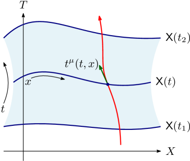
Figure 1: Depicted is a smooth one-parameter family of spacelike hypersurfaces $\mathsf{X}(t)$ that define a foliation of Minkowski space, $\mathcal{F}\mathrel{\mathchoice{\vbox{\hbox{$\displaystyle:$}}}{\vbox{\hbox{$\textstyle:$}}}{\vbox{\hbox{$\scriptstyle:$}}}{\vbox{\hbox{$\scriptscriptstyle:$}}}{=}}\{\mathsf{X}(t),\ \forall t\in[t_{1},t_{2}]\}$. The parameter $x$ is a spatial coordinate parameterizing each hypersurface (blue), and $t^{\mu}(t,x)$ denotes the deformation vector field (green), defined in Eq. (2), which is tangent to integral curves (red) associated with the $\mathcal{F}$.

III Dirac Quantization of PFT

While it is true that the gauge-invariant dynamics defined by the action in Eq. (3) coincides with the dynamics defined by the action Eq. (1), the former is defined on an extended configuration space that explicitly includes degrees of freedom associated with an embedding relative to which the scalar field is to be described. However, the embedding degrees of freedom are not independent of the matter field degrees of freedom due to the constraints in Eq. (4).

Quantization proceeds via the Dirac prescription by promoting the configuration variables, $X^{\mu}(x)$ and $\phi(x)$, and their conjugate momenta, $\Pi_{\mu}(x)$ and $\pi(x)$, to operators satisfying canonical commutation relations on the kinematical Hilbert space $\mathcal{H}_{\rm kin}\simeq\mathcal{H}_{\rm Emb}\otimes\mathcal{H}_{\phi}$, where $\mathcal{H}_{\rm Emb}$ and $\mathcal{H}_{\phi}$ are the kinematical embedding and matter field Hilbert spaces, respectively. These canonical phase space operators then define a quantization of the constraint operator in Eq. (4) upon a choice of factor ordering and regularization. Physical states are defined as those that are annihilated by the constraint operator and used to construct the physical Hilbert space $\mathcal{H}_{\rm phys}$. We outline the formal construction of $\mathcal{H}_{\phi}$, $\mathcal{H}_{\rm Emb}$, and $\mathcal{H}_{\rm phys}$, and introduce structures necessary for a field-theoretic generalization of the Page-Wootters formalism.

III.1 The matter field Hilbert space $\mathcal{H}_{\phi}$

As a minimal assumption, take the classical configuration space of the matter field $\mathcal{C}_{\phi}=\{\phi(x)\}$ to be the space of twice differentiable functions that decay rapidly at infinity on the hypersurface $\mathsf{X}$. By analogy with the quantum description of a nonrelativistic free particle, where the Hilbert space is the space of square-integrable functions over the configuration space $\mathbb{R}^{3}$, one would naïvely expect that the Hilbert space of the matter field to be $\mathcal{H}_{\phi}\simeq L^{2}(\mathcal{C}_{\phi},\mathcal{D}\phi)$ for some measure $\mathcal{D}\phi$. However, the field configuration space $\mathcal{C}_{\phi}$ is infinite-dimensional, complicating the integration theory necessary to define $\mathcal{H}_{\phi}$. To address these issues, we follow the construction of $\mathcal{H}_{\phi}$ presented in Refs. Glimm and Jaffe (1981); Ashtekar et al. (1994); Ashtekar and Lewandowski (2004); Ticciati (1999).

One proceeds by introducing an arbitrary, linearly independent set of probe functions $V=\{v_{1}(x),\dots,v_{n}(x)\}$ that are elements of the Schwartz space $\mathcal{S}$ of smooth, rapidly decreasing functions on $\mathbb{R}$. These functions probe the structure of the field configuration space through the linear functionals constructed by smearing the field operators on $\Sigma$

$$\phi_{i}\mathrel{\mathchoice{\vbox{\hbox{$\displaystyle:$}}}{\vbox{\hbox{$\textstyle:$}}}{\vbox{\hbox{$\scriptstyle:$}}}{\vbox{\hbox{$\scriptscriptstyle:$}}}{=}}\int d\Sigma(x)\,v_{i}(x)\phi(x),$$

where $d\Sigma(x)\mathrel{\mathchoice{\vbox{\hbox{$\displaystyle:$}}}{\vbox{\hbox{$\textstyle:$}}}{\vbox{\hbox{$\scriptstyle:$}}}{\vbox{\hbox{$\scriptscriptstyle:$}}}{=}}dx\sqrt{\gamma(x)}$ is the invariant measure on $\Sigma$ and $\gamma(x)\mathrel{\mathchoice{\vbox{\hbox{$\displaystyle:$}}}{\vbox{\hbox{$\textstyle:$}}}{\vbox{\hbox{$\scriptstyle:$}}}{\vbox{\hbox{$\scriptscriptstyle:$}}}{=}}\eta_{\mu\nu}\partial_{x}X^{\mu}(x)\partial_{x}X^{\nu}(x)$ is both the induced metric on $\Sigma$ and its determinant; the numbers $\phi_{i}$ can be interpreted as the component of the field along $v_{i}$. One then defines the set $\mathrm{Cyl}_{V}$ of so-called cylindrical functions on $\mathcal{C}_{\phi}$ with respect to $V$ as those that can be expressed as functions of the coordinates $\phi_{i}$,

$$f(\phi)=f(\phi_{1},\dots,\phi_{n})\in\mathrm{Cyl}_{V},$$ (6)

i.e. functions that are constant along the other directions in $\mathcal{C}_{\phi}$ (not encompassed by the probes), and introduces an inner product on $\mathrm{Cyl}_{V}$

$$\braket{f,g}\mathrel{\mathchoice{\vbox{\hbox{$\displaystyle:$}}}{\vbox{\hbox{$\textstyle:$}}}{\vbox{\hbox{$\scriptstyle:$}}}{\vbox{\hbox{$\scriptscriptstyle:$}}}{=}}\int d\mu_{n}\,f^{*}(\phi_{1},\dots,\phi_{n})g(\phi_{1},\dots,\phi_{n}),$$ (7)

where $d\mu_{n}$ is a measure on $\mathbb{R}^{n}$. The space $\mathrm{Cyl}_{V}$ is then extended to the space $\mathrm{Cyl}$ of all functions that are cylindrical with respect to some set of probes, not necessarily the set $V$. For the inner product in Eq. (7) to be well-defined, the value of the integral cannot depend on the specific set of probes used to represent the functions. This imposes nontrivial consistency requirements on the measure $d\mu_{n}$ on $\mathrm{Cyl}$ that can be met, for example, by a normalized Gaussian measure on $\mathbb{R}^{n}$. The Cauchy completion of $\mathrm{Cyl}$ with respect to the norm induced by Eq. (7) is taken to be the Hilbert space of the field $\mathcal{H}_{\phi}$. One can then extend the measure $\mathcal{D}\phi\mathrel{\mathchoice{\vbox{\hbox{$\displaystyle:$}}}{\vbox{\hbox{$\textstyle:$}}}{\vbox{\hbox{$\scriptstyle:$}}}{\vbox{\hbox{$\scriptscriptstyle:$}}}{=}}\lim_{n\to\infty}d\mu_{n}$ onto the space of tempered distributions $\mathcal{S}^{\prime}$, which is the topological dual of the Schwartz space of probes $\mathcal{S}$ (i.e., the space of linear functionals on $\mathcal{S}$), and show that $\mathcal{H}_{\phi}\simeq L^{2}(\mathcal{S}^{\prime},\mathcal{D}\phi)$; for this reason, $\mathcal{S}^{\prime}\supset\mathcal{C}_{\phi}$ is known as the quantum configuration space, which is larger than $\mathcal{C}_{\phi}$ Ashtekar et al. (1994); Ashtekar and Lewandowski (2004). In that way, it encodes the distributional character of quantum field theory.

Having defined the Hilbert space $\mathcal{H}_{\phi}$, we seek a representation of the field operator, its conjugate momentum, and their canonical commutation relations. Analogous to the generalized eigenstates of the position operator in nonrelativistic quantum mechanics, we can define generalized field eigenstates $\ket{\phi}$ associated with configurations of the field $\phi(x)\in\mathcal{S}^{\prime}$. More specifically, consider the distributional field operator $\hat{\phi}(x)$ on a hypersurface $\mathsf{X}$ satisfying

$$\hat{\phi}(x)\ket{\phi}=\phi(x)\ket{\phi}.$$

The states $\ket{\phi}$ can be represented as a delta functional on $\mathcal{S}^{\prime}$,

$$\ket{\phi}=\int_{\mathcal{S}^{\prime}}\mathcal{D}\phi^{\prime}\,\delta[\phi-\phi^{\prime}]\ket{\phi^{\prime}},$$

and are orthogonal to one another $\braket{\phi}{\phi^{\prime}}=\delta[\phi-\phi^{\prime}]$. It follows that these states form a basis for $\mathcal{H}_{\phi}$, so that any field state on $\mathsf{X}$ may be expanded as

$$\ket{\Psi_{\phi}}=\int_{\mathcal{S}^{\prime}}\mathcal{D}\phi\,\Psi_{\phi}[\phi]\ket{\phi},$$

where $\Psi_{\phi}[\phi]=\braket{\phi}{\Psi_{\phi}}\in\mathcal{H}_{\phi}$.

It will be useful to smear the distributional field operator with a probe function $f\in\mathcal{S}$,

$$\hat{\phi}[f]\mathrel{\mathchoice{\vbox{\hbox{$\displaystyle:$}}}{\vbox{\hbox{$\textstyle:$}}}{\vbox{\hbox{$\scriptstyle:$}}}{\vbox{\hbox{$\scriptscriptstyle:$}}}{=}}\int d\Sigma(x)\,f(x)\hat{\phi}(x),$$

and define its conjugate momentum

$$\hat{\pi}[g]\mathrel{\mathchoice{\vbox{\hbox{$\displaystyle:$}}}{\vbox{\hbox{$\textstyle:$}}}{\vbox{\hbox{$\scriptstyle:$}}}{\vbox{\hbox{$\scriptscriptstyle:$}}}{=}}-i\int_{\mathcal{S}^{\prime}}\mathcal{D}\phi\int d\Sigma(x)\,g(x)\ket{\phi}\frac{\delta}{\delta\phi(x)}\bra{\phi},$$

which together furnish a representation of the canonical commutation relations

$$\left[\hat{\phi}[f],\hat{\pi}[g]\right]\ket{\Psi_{\phi}}=i\left(\int d\Sigma(x)f(x)g(x)\right)\ket{\Psi_{\phi}}.$$

III.2 The embedding field Hilbert space $\mathcal{H}_{\rm Emb}$

III.2.1 General framework

The embedding field Hilbert space $\mathcal{H}_{\rm Emb}$ ought to be defined as the space of square-integrable functions over the configuration space of the embedding fields $Q$ containing all possible hypersurfaces, $\mathsf{X}:\Sigma\to\mathcal{M}\in\text{Emb}(\Sigma,\mathcal{M})$. This is a mathematically subtle topic because $\text{Emb}(\Sigma,\mathcal{M})$ is not a vector space (one cannot add arbitrary embeddings to form another one), and we shall invoke a few assumptions to proceed in analogy to the construction of the scalar field Hilbert space. Following Isham and Kuchař Isham and Kuchař (1985b, a), we first consider the space of all (not necessarily spacelike) embeddings $\text{Emb}:\Sigma\to\mathcal{M}$, where $\Sigma=\mathbb{R}$. We then take the configuration space to be

$$Q\mathrel{\mathchoice{\vbox{\hbox{$\displaystyle:$}}}{\vbox{\hbox{$\textstyle:$}}}{\vbox{\hbox{$\scriptstyle:$}}}{\vbox{\hbox{$\scriptscriptstyle:$}}}{=}}\text{Emb}(\Sigma,\mathcal{M})/\text{Diff}(\Sigma)\simeq G/H,$$

where $G\mathrel{\mathchoice{\vbox{\hbox{$\displaystyle:$}}}{\vbox{\hbox{$\textstyle:$}}}{\vbox{\hbox{$\scriptstyle:$}}}{\vbox{\hbox{$\scriptscriptstyle:$}}}{=}}\text{Diff}(\mathcal{M})$ is the group of diffeomorphisms on $\mathcal{M}$, $H\mathrel{\mathchoice{\vbox{\hbox{$\displaystyle:$}}}{\vbox{\hbox{$\textstyle:$}}}{\vbox{\hbox{$\scriptstyle:$}}}{\vbox{\hbox{$\scriptscriptstyle:$}}}{=}}\text{Diff}(\mathcal{M},\mathsf{X}_{0})$ is the subgroup of diffeomorphisms that leave invariant a fiducial embedding $\mathsf{X}_{0}:\Sigma\to\mathcal{M}$, and $\text{Diff}(\Sigma)$ is the group of diffeomorphisms on $\Sigma$. The embedding field Hilbert space will then be $\mathcal{H}_{\rm emb}\simeq L^{2}(\tilde{Q},\mathcal{D}q)$ for an appropriate measure $\mathcal{D}q$ on the quantum configuration space $\tilde{Q}\supset Q$.

The embedding fields are assumed to be promoted to self-adjoint operators on $\mathcal{H}_{\rm Emb}$ defined by the eigenvalue-eigenvector equation

$$\hat{X}^{\mu}(x)\ket{\mathsf{X}_{q}}\mathrel{\mathchoice{\vbox{\hbox{$\displaystyle:$}}}{\vbox{\hbox{$\textstyle:$}}}{\vbox{\hbox{$\scriptstyle:$}}}{\vbox{\hbox{$\scriptscriptstyle:$}}}{=}}X_{q}^{\mu}(x)\ket{\mathsf{X}_{q}},$$

where $X_{q}^{\mu}(x):\Sigma\to\mathcal{M}$ is the eigenfunction corresponding to the generalized eigenstate $\ket{\mathsf{X}_{q}}$ and equal to the coordinate functions describing the embedding $\mathsf{X}_{q}$.

Given that the embedding field operators are taken to be self-adjoint, the embedding operator $\hat{X}^{\mu}(x)$ is densely defined on the basis $\ket{\mathsf{X}_{q}}$, which are generalized eigenstates of the embedding operator $\hat{X}^{\mu}(x)$ with real eigenvalue functions $X^{\mu}_{q}(x)$. This is consistent with the demand that $\hat{X}^{\mu}(x)$ is self-adjoint and thus $\ket{\mathsf{X}_{q}}$ are orthogonal for different $q$, so that we may represent hypersurface states as Dirac delta functionals

$$\ket{\mathsf{X}_{q}}=\int\mathcal{D}q^{\prime}\,\delta[\mathsf{X}_{q^{\prime}}-\mathsf{X}_{q}]\ket{\mathsf{X}_{q^{\prime}}}.$$

It follows that $\{\ket{\mathsf{X}_{q}},\ \forall q\in\tilde{Q}\}$ forms a basis for $\mathcal{H}_{\rm Emb}$, and thus we have a resolution of the identity

$$\hat{I}_{\rm Emb}=\int\mathcal{D}q\,\ket{\mathsf{X}_{q}}\!\bra{\mathsf{X}_{q}},$$ (8)

and we can expand embedding states as

$$\ket{\psi}=\int\mathcal{D}q\,\psi[\mathsf{X}_{q}]\ket{\mathsf{X}_{q}},$$

where $\psi[\mathsf{X}_{q}]\mathrel{\mathchoice{\vbox{\hbox{$\displaystyle:$}}}{\vbox{\hbox{$\textstyle:$}}}{\vbox{\hbox{$\scriptstyle:$}}}{\vbox{\hbox{$\scriptscriptstyle:$}}}{=}}\braket{\mathsf{X}_{q}}{\psi}$.

The embedding operators $\hat{X}^{\mu}(x)$ may be smeared with a one-form $w_{\mu}(x)$ on $\Sigma$, yielding

$$\hat{\mathsf{X}}[w] \mathrel{\mathchoice{\vbox{\hbox{$\displaystyle:$}}}{\vbox{\hbox{$\textstyle:$}}}{\vbox{\hbox{$\scriptstyle:$}}}{\vbox{\hbox{$\scriptscriptstyle:$}}}{=}}\int d\Sigma(x)\,w_{\mu}(x)\hat{X}^{\mu}(x)$$

$$=\int d\Sigma(x)\,w_{\mu}(x)\int\mathcal{D}q\,\ket{\mathsf{X}_{q}}{X}_{q}^{\mu}(x)\bra{\mathsf{X}_{q}}.$$

The momentum operator canonically conjugate to $\hat{\mathsf{X}}[w]$ can be represented as

$$\hat{\mathsf{\Pi}}[v] \mathrel{\mathchoice{\vbox{\hbox{$\displaystyle:$}}}{\vbox{\hbox{$\textstyle:$}}}{\vbox{\hbox{$\scriptstyle:$}}}{\vbox{\hbox{$\scriptscriptstyle:$}}}{=}}\int d\Sigma(x)\,v^{\mu}(x)\hat{\Pi}_{\mu}(x)$$

$$=-i\int d\Sigma(x)\,v^{\mu}(x)\int\mathcal{D}q\ket{\mathsf{X}_{q}}\frac{\delta}{\delta X_{q}^{\mu}(x)}\bra{\mathsf{X}_{q}},$$

where $v^{\mu}(x)$ is a vector field on $\Sigma$. Together, these operators furnish a representation of the canonical commutation relations

$$\left[\hat{\mathsf{X}}[w],\hat{\mathsf{\Pi}}[v]\right]=i\int d\Sigma(x)\,w_{\mu}(x)v^{\mu}(x).$$

Note that $\hat{\mathsf{\Pi}}[v]$ cannot be a self-adjoint operator in general. If this were the case, then the canonical commutation relation would imply that the embedding configuration space has a linear structure and would thus be a vector space. However, this is not true, as one cannot add arbitrary embeddings to produce another embedding (see Isham and Kuchař (1985a, b) for further discussion). Nevertheless, because $\hat{\mathsf{\Pi}}[v]$ is symmetric, for different vector fields $v^{\mu}$ it will have non-trivial domains in $\mathcal{H}_{\rm emb}$, where it may effectively act like a self-adjoint operator. On these domains it will act like a translation operator for the embedding fields, however, only locally in the embedding configuration space.

III.2.2 Coherent states relative to subgroups of spacetime diffeomorphisms

Consider a representation of a one-dimensional subgroup $G_{v}\subset\mathrm{Diff}(\mathcal{M})$ generated by the vector field $v^{\mu}(x)\in\mathrm{Vec}(\mathcal{M})$, which is taken to vanish asymptotically, given by

$$\hat{U}_{v}(s)\mathrel{\mathchoice{\vbox{\hbox{$\displaystyle:$}}}{\vbox{\hbox{$\textstyle:$}}}{\vbox{\hbox{$\scriptstyle:$}}}{\vbox{\hbox{$\scriptscriptstyle:$}}}{=}}e^{-is\hat{\mathsf{\Pi}}[v]}=e^{-is\int d\Sigma(x)\,v^{\mu}(x)\hat{\Pi}_{\mu}(x)},$$ (9)

for all $s\in[s_{0},s_{1}]\subset\mathbb{R}$, where this interval will depend on the states this operator acts on. For some (possibly distributional) states it may even be defined for all $s\in\mathbb{R}$. On the domain of $\hat{\mathsf{\Pi}}[v]$, this group representation will effectively act unitarily. Let us now consider a seed state $\ket{\mathsf{X}_{0}}$, taken to be a generalized eigenstate of the embedding field operator which thus corresponds to a definite hypersurface configuration, and define the set of group coherent states Perelomov (1986) generated by the action of $\hat{U}_{v}(s)$:

$$\left\{\ket{\mathsf{X}_{v}(s)}\mathrel{\mathchoice{\vbox{\hbox{$\displaystyle:$}}}{\vbox{\hbox{$\textstyle:$}}}{\vbox{\hbox{$\scriptstyle:$}}}{\vbox{\hbox{$\scriptscriptstyle:$}}}{=}}\hat{U}_{v}(s)\ket{\mathsf{X}_{0}}\mbox{ for all }s\in[s_{0},s_{1}]\subset\mathbb{R}\right\}\,,$$ (10)

where the interval $[s_{0},s_{1}]$ depends on $\mathsf{X}_{0}$. Similarly defined coherent states relative to subgroups of the diffeomorphism group of Euclidean space have found application in general quantization methods Twareque Ali and Goldin (1991). As shown in Appendix A.1, these coherent states satisfy

$$\hat{X}^{\mu}(x)\ket{\mathsf{X}_{v}(s)} =\Big{(}X_{0}^{\mu}(x)+sv^{\mu}(x)\Big{)}\ket{\mathsf{X}_{v}(s)}.$$ (11)

This yields an interpretation of $\ket{\mathsf{X}_{v}(s)}$ as a state of the embedding fields associated with a hypersurface described by the coordinate functions $X^{\mu}(x)=X_{0}^{\mu}(x)+sv^{\mu}(x)$, where $X_{0}^{\mu}(x)$ are the coordinate functions of the seed hypersurface $\mathsf{X}_{0}$; see Fig. 2.

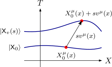
Figure 2: Hypersurfaces corresponding the seed state $\ket{\mathsf{X}_{0}}$ and the state $\ket{\mathsf{X}_{v}(s)}\mathrel{\mathchoice{\vbox{\hbox{$\displaystyle:$}}}{\vbox{\hbox{$\textstyle:$}}}{\vbox{\hbox{$\scriptstyle:$}}}{\vbox{\hbox{$\scriptscriptstyle:$}}}{=}}\hat{U}_{v}(s)\ket{\mathsf{X}_{0}}$, which is connected to the seed embedding by a unitary representation $\hat{U}_{v}(s)$ of the one-dimensional subgroup $G_{v}\subset\mathrm{Diff}(\mathcal{M})$ generated by the vector field $v^{\mu}(x)\in\mathrm{Vec}(\mathcal{M})$.

III.3 The physical Hilbert space $\mathcal{H}_{\rm phys}$

Physical states $\ket{\Psi_{\rm phys}}$ are defined as those living in the kernel of the constraint operators resulting from the quantization of Eq. (4):

$$\hat{C}_{\mu}(x)\ket{\Psi_{\rm phys}}=\left(\hat{\Pi}_{\mu}(x)+\hat{h}_{\mu}(x)\right)\ket{\Psi_{\rm phys}}=0,$$ (12)

where

$$\hat{h}_{\mu}(x)\mathrel{\mathchoice{\vbox{\hbox{$\displaystyle:$}}}{\vbox{\hbox{$\textstyle:$}}}{\vbox{\hbox{$\scriptstyle:$}}}{\vbox{\hbox{$\scriptscriptstyle:$}}}{=}}\hat{n}_{\nu}(x)\otimes{\hat{T}^{\nu}}_{\ \mu}(x)+\hat{A}_{\mu}(x)$$ (13)

is the quantization of the Hamiltonian flux in Eq. (5), which picks up an anomalous term

$$\hat{A}_{\mu}(x)\!=\!-\!\int\mathcal{D}q\,\ket{\mathsf{X}_{q}}\sqrt{\gamma(x)}\!\left(\!\eta_{\mu\nu}X_{q}^{\nu}(x)\frac{\partial\mathcal{K}}{\partial x}\!-\!\mathcal{K}^{2}n_{\mu}\!\right)\!\bra{\mathsf{X}_{q}},$$

if we consider a free scalar field theory, i.e. one with mass $m=0$. In that case, we are dealing with a conformal field theory (CFT) which leads to anomalies in the quantum setting. Adding the anomaly to the Hamiltonian ensures the constraint algebra closes Kuchař (1989b), and is further discussed in Appendix C. In the expression above, $\mathcal{K}$ represents the trace of the extrinsic curvature of the embedding $\mathsf{X}_{q}$. The effect of this anomalous term is to redistribute the energy content of the slice based on how it is embedded in the higher dimensional spacetime Kuchař (1989b). Notice that when acting on states with support only on flat embeddings, the anomalous term vanishes, as such embeddings have constant zero extrinsic curvature. One should also keep in mind that if the embeddings are taken to be flat at infinity, the anomaly vanishes when integrated over the entire spacelike slice (in any coordinate frame)

$$\int d\Sigma_{q}(x)\,\hat{A}_{\mu}(x)=0.$$ (14)

If the embedding states $\ket{\mathsf{X}_{v}(s)}$ in Eq. (10) are generated from an asymptotically flat embedding $\mathsf{X}_{0}$, then the anomaly vanishes when integrated over the associated hypersurface $\mathsf{X}_{v}(s)$.

We assume that the set of states satisfying Eq. (12) can be equipped with an inner product and completed to form the physical Hilbert space $\mathcal{H}_{\rm phys}$. Gauge transformations are generated by $\hat{\mathsf{C}}[v]\mathrel{\mathchoice{\vbox{\hbox{$\displaystyle:$}}}{\vbox{\hbox{$\textstyle:$}}}{\vbox{\hbox{$\scriptstyle:$}}}{\vbox{\hbox{$\scriptscriptstyle:$}}}{=}}\hat{\mathsf{\Pi}}[v]+\hat{\mathsf{h}}[v]$ and leave physical states invariant, $e^{i\hat{\mathsf{C}}[v]}\ket{\Psi_{\rm phys}}=\ket{\Psi_{\rm phys}}$, for all $\ket{\Psi_{\rm phys}}\in\mathcal{H}_{\rm phys}$.

IV Matter relative to quantum fields

When reparametrization-invariant theories are canonically quantized, it is found that the Hamiltonian of the theory is proportional to a constraint operator. This implies that physical states do not evolve under the action generated by the quantized Hamiltonian. This is a generic feature of relativistic theories and, ultimately, a manifestation of background independence. This means that there is no physical evolution relative to the external background.

Nonetheless, we are tasked with recovering a notion of dynamics from the quantized theory. One approach is to identify a subsystem after quantization to serve as a reference frame relative to which another subsystem evolves. Three approaches that accomplish this task are the construction of so-called relational Dirac observables (a.k.a., evolving constants of motion) Rovelli (2004); Dittrich (2006, 2007); Thiemann (2008), the Page and Wootters formalism Page and Wootters (1983); Wootters (1984), and a quantum deparametrization procedure Höhn and Vanrietvelde (2020); Höhn (2019). For simple mechanical systems, these approaches have been shown to be equivalent in Höhn et al. (2021a, b).

In this section, we introduce the Page-Wootters formulation of the parameterized field theory reviewed in Sec. II. A conditional state of the matter field is defined by conditioning physical states on configurations of the embedding fields. This conditional state is then shown to formally satisfy the covariant Tomonaga-Schwinger equation and an appropriate Schrödinger equation describing evolution along arbitrary spacelike foliations of Minkowski space, thus demonstrating the formal equivalence of the Page-Wootters formalism with standard formulations of quantum field theory. We also introduce relational Dirac observables and a quantum deparameterization of the physical Hilbert space that results in a relational Heisenberg picture. These relational formulations are shown to be unitarily equivalent to the Page-Wootters formalism.

IV.1 The Page-Wootters formalism and Tomonaga-Schwinger equation

The typical starting point of the Page-Wootters formalism applied to a mechanical system is a physical state $\ket{\Psi_{\rm phys}}$ describing a non-interacting clock $C$ and system of interest $S$ satisfying a Hamiltonian constraint

$$\hat{C}_{H}\ket{\Psi_{\rm phys}}=\left(\hat{H}_{C}+\hat{H}_{S}\right)\ket{\Psi_{\rm phys}}=0.$$ (15)

One then considers a time observable

$$T_{C}\mathrel{\mathchoice{\vbox{\hbox{$\displaystyle:$}}}{\vbox{\hbox{$\textstyle:$}}}{\vbox{\hbox{$\scriptstyle:$}}}{\vbox{\hbox{$\scriptscriptstyle:$}}}{=}}\{\ket{t}\!\bra{t},\ \forall t\in G\subseteq\mathbb{R}\},$$

defined by a set of rank-1 effect density operators $\ket{t}\!\bra{t}$ constructed from the outer product of so-called clock states $\ket{t}$ for all $t\in\mathbb{R}$ that parameterize the one-dimensional time evolution group $G$ generated by the clock Hamiltonian $\hat{H}_{C}$. What distinguishes $T_{C}$ as a time observable is that it transforms covariantly under the action of $G$, which amounts to the following relation between the clock states

$$\ket{t^{\prime}}=e^{-i\hat{H}_{C}\left(t^{\prime}-t\right)}\ket{t}.$$ (16)

One then defines the conditional state of the system $\ket{\psi_{S}(t)}$ at a time $t$ as

$$\ket{\psi_{S}(t)}\mathrel{\mathchoice{\vbox{\hbox{$\displaystyle:$}}}{\vbox{\hbox{$\textstyle:$}}}{\vbox{\hbox{$\scriptstyle:$}}}{\vbox{\hbox{$\scriptscriptstyle:$}}}{=}}\left(\bra{t}\otimes\hat{I}_{S}\right)\ket{\Psi_{\rm phys}}.$$ (17)

It then follows from Eqs. (15) and (16) that the conditional wave function satisfies the Schrödinger equation, $i\frac{d}{dt}\ket{\psi_{S}(t)}=\hat{H}_{S}\ket{\psi_{S}(t)}$, and yields the correct one- and two-time probabilities Höhn et al. (2021a). Thus, we conclude that the conditional state $\ket{\psi_{S}(t)}$ ought to be interpreted as the usual time-dependent solution to the Schrödinger equation, which constitutes the recovery of the standard quantum mechanical framework from the Page-Wootters formalism.

However, Page and Wootters never intended these ideas to be limited to mechanical systems, which is made clear when Page writes Page (1989):

‘For simplicity, one can think of the […] system as a “particle” with “position”, which is a convenient model to have in mind, but my discussion is not intended to be limited to such a simple model. For example, the closed system could consist of relativistic quantum fields within a given classical background spacetime.’

Taking this seriously, we develop a field-theoretic generalization of the Page-Wootters formalism for PFT. We begin by considering a physical state $\ket{\Psi_{\rm phys}}$ satisfying Eq. (12), and introducing the so-called reduction map $\mathcal{R}_{\mathbf{S}}[\mathsf{X}_{q}]$, which plays the same role as Eq. (17). The reduction map is defined as

$$\begin{split}\mathcal{R}_{\mathbf{S}}[\mathsf{X}_{q}]:\mathcal{H}_{\rm phys}&\rightarrow\mathcal{H}_{\mathsf{X}_{q}},\\ \ \ket{\Psi_{\rm phys}}&\mapsto\ket{\psi_{\phi}[\mathsf{X}_{q}]}\mathrel{\mathchoice{\vbox{\hbox{$\displaystyle:$}}}{\vbox{\hbox{$\textstyle:$}}}{\vbox{\hbox{$\scriptstyle:$}}}{\vbox{\hbox{$\scriptscriptstyle:$}}}{=}}\mathcal{R}_{\mathbf{S}}[\mathsf{X}_{q}]\ket{\Psi_{\rm phys}},\end{split}$$

where

$$\mathcal{R}_{\mathbf{S}}[\mathsf{X}_{q}]\mathrel{\mathchoice{\vbox{\hbox{$\displaystyle:$}}}{\vbox{\hbox{$\textstyle:$}}}{\vbox{\hbox{$\scriptstyle:$}}}{\vbox{\hbox{$\scriptscriptstyle:$}}}{=}}\bra{\mathsf{X}_{q}}\otimes\hat{I}_{\phi},$$ (18)

is used to condition a physical state $\ket{\Psi_{\rm phys}}$ on an embedding state $\ket{\mathsf{X}_{q}}$. We refer to $\ket{\psi_{\phi}[\mathsf{X}_{q}]}$ as a conditional state of the field $\phi$ relative to the hypersurface $\mathsf{X}_{q}$.

As a consequence of the resolution of the identity in Eq. (8), the reduction map is formally invertible on physical states, with inverse

$$\mathcal{R}^{-1}_{\mathbf{S}}[\mathsf{X}_{q}]:\mathcal{H}_{\mathsf{X}_{q}} \rightarrow\mathcal{H}_{\rm phys};$$

$$\ \ket{\psi_{\phi}[\mathsf{X}_{q}]} \mapsto\ket{\Psi_{\rm phys}}=\mathcal{R}^{-1}_{\mathbf{S}}[\mathsf{X}_{q}]\ket{\psi_{\phi}[\mathsf{X}_{q}]},$$

where

$$\mathcal{R}_{\mathbf{S}}^{-1}[\mathsf{X}_{q}] =\int\mathcal{D}q^{\prime}\,\ket{\mathsf{X}_{q^{\prime}}}\otimes\hat{U}_{\phi}[\mathsf{X}_{q^{\prime}}-\mathsf{X}_{q}]$$ (19)

$$=\int\mathcal{D}q^{\prime}\,\hat{U}_{\mathsf{X}}[\mathsf{X}_{q^{\prime}}-\mathsf{X}_{q}]\ket{\mathsf{X}_{q}}\otimes\hat{U}_{\phi}[\mathsf{X}_{q^{\prime}}-\mathsf{X}_{q}],$$

and

$$\hat{U}_{\mathsf{X}}[\mathsf{X}_{q^{\prime}}-\mathsf{X}_{q}] \mathrel{\mathchoice{\vbox{\hbox{$\displaystyle:$}}}{\vbox{\hbox{$\textstyle:$}}}{\vbox{\hbox{$\scriptstyle:$}}}{\vbox{\hbox{$\scriptscriptstyle:$}}}{=}}e^{-i\int d\Sigma_{q}(x)\,\left(X^{\mu}_{q^{\prime}}(x)-X^{\mu}_{q}(x)\right)\hat{\Pi}_{\mu}(x)},$$

$$\hat{U}_{\phi}[\mathsf{X}_{q^{\prime}}-\mathsf{X}_{q}] \mathrel{\mathchoice{\vbox{\hbox{$\displaystyle:$}}}{\vbox{\hbox{$\textstyle:$}}}{\vbox{\hbox{$\scriptstyle:$}}}{\vbox{\hbox{$\scriptscriptstyle:$}}}{=}}e^{-i\int d\Sigma_{q}(x)\,\left(X^{\mu}_{q^{\prime}}(x)-X^{\mu}_{q}(x)\right)n_{\nu}(x){\hat{T}^{\nu}}_{\ \mu}(x)}.$$ (20)

Note that the surface integrals above are defined on the embedded hypersurface $\mathsf{X}_{q}$ in Minkowski space and that the difference $X^{\mu}_{q^{\prime}}(x)-X^{\mu}_{q}(x)$ defines a vector field on (but not necessarily tangential to) this surface. In the line above, $n_{\nu}(x)$ is no longer an operator as it has already been evaluated on the embedding $\mathsf{X}_{q}$. The action of the inverse map on a conditional state of the field is then

$$\mathcal{R}_{\mathbf{S}}^{-1}[\mathsf{X}_{q}]\ket{\psi_{\phi}[\mathsf{X}_{q}]}=\int\mathcal{D}q\,\ket{\mathsf{X}_{q}}\ket{\psi_{\phi}[\mathsf{X}_{q}]}=\ket{\Psi_{\rm phys}}.$$ (21)

Given that $\mathcal{R}_{\mathbf{S}}[\mathsf{X}_{q}]$ is invertible, it follows that $\mathcal{H}_{\rm phys}$ is isomorphic to $\mathcal{H}_{\mathsf{X}_{q}}$.

We will now consider the conditional state of the field

$$\ket{\psi_{\phi}[\mathsf{X}_{v}(s)]}\mathrel{\mathchoice{\vbox{\hbox{$\displaystyle:$}}}{\vbox{\hbox{$\textstyle:$}}}{\vbox{\hbox{$\scriptstyle:$}}}{\vbox{\hbox{$\scriptscriptstyle:$}}}{=}}\mathcal{R}_{\mathbf{S}}[\mathsf{X}_{v}(s)]\ket{\Psi_{\rm phys}}.$$ (22)

associated with a one-dimensional subgroup $G_{v}\subset G$ defined by the vector field $v^{\mu}(x)$ and group element $s$. In what follows, we will derive the variation of $\ket{\psi_{\phi}[\mathsf{X}_{v}(s)]}$ in the parameter $s$, parameterizing the subgroup $G_{v}$, and then its variation in the vector field $v^{\mu}(x)$, characterizing deformations of the hypersurface $\mathsf{X}_{0}$. We then consider the evolution of the conditional state along a foliation $\mathcal{F}$ of $\mathcal{M}$.

IV.1.1 Evolution in the group parameter $s$

One notable difference to the quantum mechanical case in Eq. (15) is that in PFT the embedding fields, serving as a dynamical reference frame for the scalar field, interacts with the scalar field via the embedding-dependent Hamiltonian in Eq. (13) (cf., Ref. Smith and Ahmadi (2019)). Nevertheless, we can proceed similarly.

The evolution of the conditional state $\ket{\psi_{\phi}[\mathsf{X}_{v}(s)]}$ in the parameter $s\in[s_{0},s_{1}]$ satisfies:

$$\begin{split}i\frac{d}{ds}\ket{\psi_{\phi}[\mathsf{X}_{v}(s)]}&=i\frac{d}{ds}\braket{\mathsf{X}_{v}(s)}{\Psi_{\rm phys}}\\ &=i\frac{d}{ds}\bra{\mathsf{X}_{0}}e^{is\hat{\mathsf{\Pi}}[v]}\ket{\Psi_{\rm phys}}\\ &=i\bra{\mathsf{X}_{0}}e^{is\hat{\mathsf{\Pi}}[v]}i\hat{\mathsf{\Pi}}[v]\ket{\Psi_{\rm phys}}\\ &=-\bra{\mathsf{X}_{v}(s)}\hat{\mathsf{\Pi}}[v]\ket{\Psi_{\rm phys}}\\ &=\bra{\mathsf{X}_{v}(s)}\hat{\mathsf{h}}[v]\ket{\Psi_{\rm phys}}\\ &=\hat{\mathsf{h}}[v,\mathsf{X}_{v}(s)]\braket{\mathsf{X}_{v}(s)}{\Psi_{\rm phys}}\\ &=\hat{\mathsf{h}}[v,\mathsf{X}_{v}(s)]\ket{\psi_{\phi}[\mathsf{X}_{v}(s)]},\end{split}$$ (23)

where the dependence on $\mathsf{X}_{v}(s)$ is through $n_{\mu}(x)$, and we have defined

$$\hat{\mathsf{h}}[v,\mathsf{X}_{v}(s)]\mathrel{\mathchoice{\vbox{\hbox{$\displaystyle:$}}}{\vbox{\hbox{$\textstyle:$}}}{\vbox{\hbox{$\scriptstyle:$}}}{\vbox{\hbox{$\scriptscriptstyle:$}}}{=}}\int d\Sigma(x)\,v^{\mu}(x)n_{\nu}(x){\hat{T}^{\nu}}_{\ \mu}(x),$$ (24)

and made use of Eqs. (9), (12), (22). It is thus seen that the operator $\hat{\mathsf{h}}[v,\mathsf{X}_{v}(s)]$ generates the flow in $s$. We remind the reader that the anomaly (when present) has vanished because we have integrated over asymptotically flat spatial hypersurfaces as in Eq. (14).

As an example, let us consider an inertial foliation of Minkowski space by flat spacelike hypersurfaces defined by the one-parameter family of hypersurfaces through the coordinate functions

$$X^{\mu}(s,x)=X^{\mu}(0,x)+sv^{\mu}(x),$$

where the fiducial embedding is taken to be $X^{\mu}(0,x)=\left(-x\sinh w,x\cosh w\right)$, the vector field $v^{\mu}(x)=\left(\cosh w,-\sinh w\right)$, and $w$ denotes the rapidity of the inertial frame moving at a relative speed $\beta$ defined as $\cosh w\mathrel{\mathchoice{\vbox{\hbox{$\displaystyle:$}}}{\vbox{\hbox{$\textstyle:$}}}{\vbox{\hbox{$\scriptstyle:$}}}{\vbox{\hbox{$\scriptscriptstyle:$}}}{=}}1/\sqrt{1-\beta^{2}}$. It then follows that

$$n_{\nu}(x)=\epsilon_{\nu\rho}\left.\frac{\partial{X}^{\rho}(x)}{\partial x}\right|_{\mathsf{X}=\mathsf{X}_{v}(s)}=(\cosh w,\sinh w),$$

which is normal to each hypersurface of the foliation. For such a foliation, Eq. (23) reduces to the Schödinger equation

$$i\frac{d}{dt}\ket{\psi_{\phi}[\mathsf{X}_{v}(t)]}=\hat{H}_{{\rm flat},\beta}\ket{\psi_{\phi}[\mathsf{X}_{v}(t)]},$$

where Eq. (24) simplifies to the Hamiltonian

$$\hat{H}_{{\rm flat},\beta}\mathrel{\mathchoice{\vbox{\hbox{$\displaystyle:$}}}{\vbox{\hbox{$\textstyle:$}}}{\vbox{\hbox{$\scriptstyle:$}}}{\vbox{\hbox{$\scriptscriptstyle:$}}}{=}}\int d\Sigma(x)\,v^{\mu}(x)n_{\nu}(x){\hat{T}^{\nu}}_{\ \mu}(x),$$

which generates an evolution in the group parameter $s=t$, interpreted as the proper time of an observer moving along the timelike congruence defined by the inertial foliation.

IV.1.2 Variation of the conditional hypersurface

Instead of considering the conditional state $\ket{\psi_{\phi}[\mathsf{X}_{v}(s)]}$ to be a function of $s$, we may instead consider it to be a functional depending on the coordinate functions $X^{\mu}(x)=X_{0}^{\mu}(s)+sv^{\mu}(x)$, where $v^{\mu}(x)$ defines a one-dimensional subgroup $G_{v}\subset\mathrm{Diff}(\mathcal{M})$ characterizing a set of particular deformations of the fiducial hypersurface $\mathsf{X}_{0}$. Let us introduce the notation $\ket{\psi_{\phi}[{X}^{\mu}(x)]}\mathrel{\mathchoice{\vbox{\hbox{$\displaystyle:$}}}{\vbox{\hbox{$\textstyle:$}}}{\vbox{\hbox{$\scriptstyle:$}}}{\vbox{\hbox{$\scriptscriptstyle:$}}}{=}}\ket{\psi_{\phi}[\mathsf{X}_{v}(s)]}$ to emphasize the functional dependence of the conditional state on the hypersurface $\mathsf{X}_{v}(s)$ through its coordinate functions ${X}^{\mu}(x)$.

Now consider variations of the conditional state under deformations of the hypersurface $\mathsf{X}_{v}(s)$ by taking the functional derivative with respect to the coordinate functions $X^{\mu}(x)$, while keeping $X_{0}^{\mu}(x)$ fixed for $s\in[s_{0},s_{1}]$:

$$i\frac{\delta\ket{\psi_{\phi}[{X}^{\mu}(x)]}}{\delta X^{\mu}(x)}\! =i\frac{\delta}{\delta X^{\mu}(x)}\braket{\mathsf{X}_{v}(s)}{\Psi_{\rm phys}}$$

$$=i\frac{\delta}{\delta X^{\mu}(x)}\bra{\mathsf{X}_{0}}e^{is\hat{\mathsf{\Pi}}[v]}\ket{\Psi_{\rm phys}}$$

$$=i\bra{\mathsf{X}_{0}}\!\frac{\delta e^{i\!\int\!d\Sigma(x)\,\left(X^{\mu}(x)-X_{0}^{\mu}(x)\right)\hat{\Pi}_{\mu}(x)}}{\delta X^{\mu}(x)}\!\ket{\Psi_{\rm phys}}$$

$$=i\bra{\mathsf{X}_{0}}e^{is\hat{\mathsf{\Pi}}[v]}i\hat{\Pi}_{\mu}(x)\ket{\Psi_{\rm phys}}$$

$$=-\bra{\mathsf{X}_{v}(s)}\hat{\Pi}_{\mu}(x)\ket{\Psi_{\rm phys}}$$

$$=\bra{\mathsf{X}_{v}(s)}\hat{h}_{\mu}(x)\ket{\Psi_{\rm phys}}$$

$$=\hat{h}_{\mu}(x,X^{\mu}(x))\ket{\psi_{\phi}[{X}^{\mu}(x)]}.$$ (25)

Let us define the surface variation as the normal projection of the functional derivative with respect to the coordinate functions Doplicher (2004)

$$\frac{\delta}{\delta\mathsf{X}(x)}\mathrel{\mathchoice{\vbox{\hbox{$\displaystyle:$}}}{\vbox{\hbox{$\textstyle:$}}}{\vbox{\hbox{$\scriptstyle:$}}}{\vbox{\hbox{$\scriptscriptstyle:$}}}{=}}n^{\mu}(x)\frac{\delta}{\delta X^{\mu}(x)},$$

where $n^{\mu}(x)$ is the normal to $\mathsf{X}_{v}(s)$; this derivative characterizes normal deformations of the conditional wave functional. By contracting Eq. (25) with $n^{\mu}(x)$, we recover the Tomonaga-Schwinger equation:

$$i\frac{\delta}{\delta\mathsf{X}(x)}\ket{\psi_{\phi}[{X}^{\mu}(x)]}=n^{\mu}(x)\hat{h}_{\mu}(x,X^{\mu}(x))\ket{\psi_{\phi}[{X}^{\mu}(x)]}.$$ (26)

The recovery of the Tomonaga-Schwinger equation equation Tomonaga (1946); Schwinger (1948); Wakita (1976); Breuer and Petruccione (2002) using the Page-Wootters formalism indicates its formal equivalence with standard functional formulations of quantum field theory. One should note that the conformal anomaly potential $\hat{A}_{\mu}(x)$ is embedded in the Hamiltonian flux (for the $m=0$ case), underlying a redistribution of the energy flux over the embedding for hypersurfaces with non-vanishing extrinsic curvature. However, this once again does not affect the integrated version of the Tomonaga-Schwinger equation, as the anomaly vanishes for asymptotically flat embeddings.

We recall that a functional Schrödinger equation has previously been derived in the context of PFT *kuchar_dirac_1989; Torre and Varadarajan (1998, 1999); Varadarajan (2007); Kaya (2023); however, not on the reduced Hilbert space of conditional states of the scalar field as done here, but rather directly using the constraint and physical states. Employing the Page-Wootters formalism here permits us to instead identify such a functional Schrödinger equation with the Tomonaga-Schwinger equation, which similarly is formulated on the Hilbert space of the quantum field alone.

IV.1.3 Schrödinger evolution along a one-parameter family of hypersurfaces

Consider a one-parameter family $\mathcal{F}\mathrel{\mathchoice{\vbox{\hbox{$\displaystyle:$}}}{\vbox{\hbox{$\textstyle:$}}}{\vbox{\hbox{$\scriptstyle:$}}}{\vbox{\hbox{$\scriptscriptstyle:$}}}{=}}\{\mathsf{X}(t),\ \forall t\in[t_{1},t_{2}]\}$ of spacelike hypersurfaces $\mathsf{X}(t)$ in Minkowski space (which may or may not constitute a foliation). Each hypersurface in the family is associated with a conditional state $\ket{\psi_{\phi}[\mathsf{X}(t)]}\mathrel{\mathchoice{\vbox{\hbox{$\displaystyle:$}}}{\vbox{\hbox{$\textstyle:$}}}{\vbox{\hbox{$\scriptstyle:$}}}{\vbox{\hbox{$\scriptscriptstyle:$}}}{=}}\mathcal{R}_{\mathbf{S}}[\mathsf{X}(t)]\ket{\Psi_{\rm phys}}$, which evolves along the family according to:

$$i\frac{d}{dt}\ket{\psi_{\phi}[\mathsf{X}(t)]} =i\lim_{\varepsilon\to 0}\frac{\ket{\psi_{\phi}[\mathsf{X}(t+\varepsilon)]}-\ket{\psi_{\phi}[\mathsf{X}(t)]}}{\varepsilon}$$

$$=i\int d\Sigma(t,x)\,t^{\mu}(t,x)\frac{\delta}{\delta{X}^{\mu}(x)}\ket{\psi_{\phi}[\mathsf{X}(t)]}$$

$$=\hat{H}(t)\,\ket{\psi_{\phi}[\mathsf{X}(t)]},$$ (27)

where we have used Eq. (25) to arrive at the last equality and defined the Hamiltonian

$$\hat{H}(t)\mathrel{\mathchoice{\vbox{\hbox{$\displaystyle:$}}}{\vbox{\hbox{$\textstyle:$}}}{\vbox{\hbox{$\scriptstyle:$}}}{\vbox{\hbox{$\scriptscriptstyle:$}}}{=}}\int d\Sigma(t,x)\,t^{\mu}(t,x)\,\hat{h}_{\mu}(x,X^{\mu}(t,x)),$$

by projecting the energy-momentum density $\hat{h}_{\mu}(x,X^{\mu}(t,x))$ along the deformation vector field $t^{\mu}$ and integrating over the Cauchy surface $\Sigma$. In particular, we can decompose the Hamiltonian into normal and parallel deformation generators:

$$\hat{H}(t)=\hat{H}_{\bot}(t)+\hat{H}_{\parallel}(t),$$

where

$$\hat{H}_{\bot}(t) \mathrel{\mathchoice{\vbox{\hbox{$\displaystyle:$}}}{\vbox{\hbox{$\textstyle:$}}}{\vbox{\hbox{$\scriptstyle:$}}}{\vbox{\hbox{$\scriptscriptstyle:$}}}{=}}\int d\Sigma(x)\,N(t)\,n^{\mu}(t,x)\,\hat{h}_{\mu}(x,X^{\mu}(t,x)),$$

$$\hat{H}_{\parallel}(t) \mathrel{\mathchoice{\vbox{\hbox{$\displaystyle:$}}}{\vbox{\hbox{$\textstyle:$}}}{\vbox{\hbox{$\scriptstyle:$}}}{\vbox{\hbox{$\scriptscriptstyle:$}}}{=}}\int d\Sigma(x)\,N^{\mu}(t,x)\,\hat{h}_{\mu}(x,X^{\mu}(t,x)).$$

It is seen that Eq. (27) constitutes a generalized Schrödinger equation that accounts for normal deformations of the hypersurface $\mathsf{X}(t)$ generated by $\hat{H}_{\perp}(t)$, and spatial redistribution of points generated by $\hat{H}_{\parallel}(t)$ (i.e., spatial diffeomorphisms of $\mathsf{X}(t)$). Moreover, the standard Schrödinger equation in Minkowski space is recovered when restricting to inertial embeddings, such as $T(t,x)=t$ and $X(t,x)=x$. It then follows that $t^{\mu}(t,x)=n^{\mu}(t,x)=(1,0)$, so that

$$i\frac{d}{dt}\ket{\psi_{\phi}[\mathsf{X}(t)]}=\hat{H}_{{\rm flat},0}\ket{\psi_{\phi}[\mathsf{X}(t)]},$$

where $\hat{H}_{{\rm flat},0}=\int d\Sigma(x)\,\hat{T}^{0}{}_{0}(x)$, is the standard Hamiltonian on a flat embedding and $\hat{T}^{0}{}_{0}(x)$ is the standard energy density in the employed coordinate frame.

Integrating Eq.(27), we arrive at

$$\ket{\psi_{\phi}[\mathsf{X}_{2}]}=\hat{U}_{\mathcal{F}}(t_{2},t_{1})\ket{\psi_{\phi}[\mathsf{X}_{1}]},$$ (28)

where

$$\hat{U}_{\mathcal{F}}(t_{2},t_{1})\mathrel{\mathchoice{\vbox{\hbox{$\displaystyle:$}}}{\vbox{\hbox{$\textstyle:$}}}{\vbox{\hbox{$\scriptstyle:$}}}{\vbox{\hbox{$\scriptscriptstyle:$}}}{=}}\mathcal{P}e^{-i\!\int_{{t_{1}}}^{{t_{2}}}\!dt\,\hat{H}(t)},$$ (29)

is formally a unitary operator that propagates the conditional state of the matter field from $\mathsf{X}_{1}$ to $\mathsf{X}_{2}$, and $\mathcal{P}$ denotes the path-ordering operator in the foliation parameter $t$. Note that the Hamiltonian density satisfies the microcausality condition, $[\hat{h}^{\mu}(t,x),\hat{h}^{\nu}(t,x^{\prime})]=0$ for spacelike separated points labeled by the coordinates $(t,x)$ and $(t,x^{\prime})$. This provides the integrability requirement for the integral in Eq. (29) to be well-defined and independent of the spacetime foliation of the region being integrated over Tomonaga (1946); Schwinger (1948); Koba (1950); Wakita (1976); Breuer and Petruccione (2002). If the Hamiltonian generating $\hat{U}_{\mathcal{F}}(t_{2},t_{1})$ is constructed by smearing the Hamiltonian flux with a deformation vector field associated with a complete spacelike foliation, then it is a complete vector field in Minkowski space $\mathcal{M}$. The deformation vector fields lifts to a complete vector field on the classical scalar field configuration space $\mathcal{C}_{\phi}$ (see Sec. III) because the deformation vector field generates a gauge diffeomorphism, which cannot change the $C^{2}$ nature of a classical field configuration, nor its asymptotic drop-off property, given that also gauge diffeomorphisms have to vanish asymptotically. In fact, this should extend to the quantum configuration space $\mathcal{S}^{\prime}$, where the action of the Lie derivative on distributions can be understood via partial integration and the properties of the gauge diffeomorphisms should ensure the preservation of the properties of the permitted set of distributions. Making this rigorous is somewhat challenging; however, it suggests that van Hove’s theorem in quantum mechanics Hove (1951); Gotay et al. (1996); Gotay (1999) could be extrapolated to field theory, in which case it would imply that the Hamiltonian is formally self-adjoint.

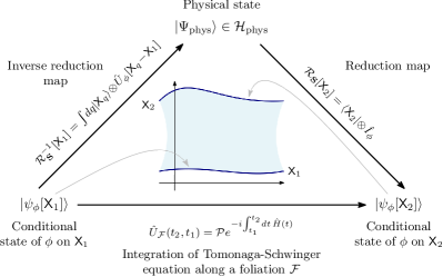
Figure 3: The composition of the inverse reduction map relative to $\mathsf{X}_{1}$ and reduction map relative to $\mathsf{X}_{2}$ (upper path), which maps the conditional state $\ket{\psi_{\phi}[\mathsf{X}_{1}]}$ to $\ket{\psi_{\phi}[\mathsf{X}_{2}]}$, is shown in Eq. (31) to be equivalent to integrating the Tomonaga-Schwinger equation along an arbitrary spacelike foliation of Minkowski space connecting $\mathsf{X}_{1}$ and $\mathsf{X}_{2}$ (lower path). Foliation-independence of the evolution of the conditional state from $\mathsf{X}_{1}$ and $\mathsf{X}_{2}$ arises in the former as a consequence of the diffeomorphisim invariance of the physical states from which the conditional states of the scalar field are constructed, while in the latter it arises as a consequence of the microcausality condition satisfied by the stress-energy tensor of the scaler field.

Alternatively, we may evolve $\ket{\psi_{\phi}[\mathsf{X}_{1}]}$ to $\ket{\psi_{\phi}[\mathsf{X}_{2}]}$ by first applying the inverse of the reduction map evaluated at $\mathsf{X}_{1}$ and then the reduction map evaluated at $\mathsf{X}_{2}$, yielding:

$$\ket{\psi_{\phi}[\mathsf{X}_{2}]} =\mathcal{R}_{\mathbf{S}}[\mathsf{X}_{2}]\circ\mathcal{R}_{\mathbf{S}}^{-1}[\mathsf{X}_{1}]\ket{\psi_{\phi}[\mathsf{X}_{1}]}$$

$$=\bra{\mathsf{X}_{2}}\otimes\hat{I}_{\phi}\int\mathcal{D}q\,\ket{\mathsf{X}_{q}}\otimes\hat{U}_{\phi}[\mathsf{X}_{q}-\mathsf{X}_{1}]\ket{\psi[\mathsf{X}_{1}]}$$

$$=\hat{U}_{\phi}[\mathsf{X}_{2}-\mathsf{X}_{1}]\ket{\psi[\mathsf{X}_{1}]}.$$ (30)

Assuming the family of hypersurfaces constitutes a foliation, applying Eq. (30) between successive leaves, as is done in Appendix B, together with the fact that $\mathcal{R}_{\mathbf{S}}^{-1}[\mathsf{X}_{q}]\circ\mathcal{R}_{\mathbf{S}}[\mathsf{X}_{q}]=\hat{I}_{\rm phys}$, which stems from the gauge invariance of physical states imposed by Eq. (12), it follows that we must have

$$\ket{\psi_{\phi}[\mathsf{X}_{2}]}=\hat{U}_{\mathcal{F}}(t_{2},t_{1})\ket{\psi_{\phi}[\mathsf{X}_{1}]}=\hat{U}_{\phi}[\mathsf{X}_{2}-\mathsf{X}_{1}]\ket{\psi_{\phi}[\mathsf{X}_{1}]}.$$ (31)

This shows that the evolution between the two hypersurfaces is formally unitary and foliation independent since neither the reduction map nor its inverse depends on $\mathcal{F}$. This is a different way of demonstrating the foliation-independence of the Tomonaga-Schwinger equation that does not use the microcausality condition but instead uses the fact that physical states are invariant under diffeomorphisms, which is a gauge symmetry of PFT. See Fig. 3 for more detail. This is an instantiation of the fact that foliation-independence and diffeomorphism invariance are deeply intertwined in canonical formulations of generally covariant theories, e.g. see Kiefer (2012); Hojman et al. (1976); Kuchar (1976a, b); Thiemann (2008).

IV.2 Changes of embedding configuration

Having constructed the conditional states $\ket{\psi_{\phi}[\mathsf{X}_{q}]}$ of the scalar field relative to an embedding $\mathsf{X}_{q}$, we now consider how the conditional state changes under a change of embedding, $\mathsf{X}_{q}\to\mathsf{X}_{q^{\prime}}$. Since the embedding fields constitute a dynamical reference frame, each configuration can be regarded as a reference frame orientation. The action of a generic change in frame configuration, $\mathsf{X}_{q}\to\mathsf{X}_{q^{\prime}}$, on the conditional state $\ket{\psi_{\phi}[\mathsf{X}_{q}]}$ is given in terms of the reduction map and its inverse, and is seen to induce a unitary map on conditional states:

$$\begin{split}\ket{\psi_{\phi}[\mathsf{X}_{q^{\prime}}]}&=\mathcal{R}_{\mathbf{S}}[\mathsf{X}_{q^{\prime}}]\circ\mathcal{R}_{\mathbf{S}}^{-1}[\mathsf{X}_{q}]\ket{\psi_{\phi}[\mathsf{X}_{q}]}\\ &=\hat{U}_{\phi}[\mathsf{X}_{q^{\prime}}-\mathsf{X}_{q}]\ket{\psi_{\phi}[\mathsf{X}_{q}]}.\end{split}$$ (32)

As depicted in Fig. 3, this map is used to transform conditional states between two embedding configurations associated with different leaves of a foliation. However, the map in Eq. (32) is more general as it maps the conditional state between two embedding configurations that are not necessarily part of a foliation. For example, consider two embedding configurations related by a finite Lorentz boost $\Lambda$. The coordinate functions characterizing these embeddings are related by $X^{\mu}_{\Lambda q}(x)={\Lambda^{\mu}}_{\nu}X^{\nu}_{q}(x)$. Inserting this in Eq. (32), we arrive at:

$$\begin{split}\ket{\psi_{\phi}[\mathsf{X}_{\Lambda q}]}&=\hat{U}_{\phi}[\mathsf{X}_{\Lambda q}-\mathsf{X}_{q}]\ket{\psi_{\phi}[\mathsf{X}_{q}]}\\ &=e^{-i\int d\Sigma(x)\,({\Lambda^{\mu}}_{\nu}-{\delta^{\mu}}_{\nu})X_{q}^{\nu}(x)\hat{h}_{\mu}(x)}\ket{\psi_{\phi}[\mathsf{X}_{q}]}.\end{split}$$

Furthermore, covariance requires that field observables $\hat{A}_{\phi}(q)$ transform between hypersurfaces $q$ and $\Lambda q$ as

$$\hat{A}_{\phi}(\Lambda q)=\hat{U}_{\phi}[\mathsf{X}_{\Lambda q}-\mathsf{X}_{q}]\hat{A}_{\phi}(q)\hat{U}^{\dagger}_{\phi}[\mathsf{X}_{\Lambda q}-\mathsf{X}_{q}].$$

We may also consider how the conditional state transforms under a transformation from an inertial to a uniformly accelerating frame Fulton et al. (1962); Wood et al. (1989). In particular, if $b^{\mu}\mathrel{\mathchoice{\vbox{\hbox{$\displaystyle:$}}}{\vbox{\hbox{$\textstyle:$}}}{\vbox{\hbox{$\scriptstyle:$}}}{\vbox{\hbox{$\scriptscriptstyle:$}}}{=}}\left(0,\frac{1}{\alpha}\right)$ is a constant vector, the embedding configuration obtained through the finite special conformal transformation $X^{\mu}_{q^{\prime}}(x)=\frac{X^{\mu}_{q}(x)-b^{\mu}X^{2}_{q}(x)}{\beta(x)}$ experiences a uniform acceleration $\alpha$ relative to $X_{q}$, where $\beta(x)\mathrel{\mathchoice{\vbox{\hbox{$\displaystyle:$}}}{\vbox{\hbox{$\textstyle:$}}}{\vbox{\hbox{$\scriptstyle:$}}}{\vbox{\hbox{$\scriptscriptstyle:$}}}{=}}2X^{\sigma}(x)b_{\sigma}-X_{q}^{\sigma}(x){X_{q}}_{\sigma}(x)/\alpha^{2}$. Using Eq. (32), the conditional state of the field transforms as

$$\begin{split}\ket{\psi_{\phi}[\mathsf{X}_{q^{\prime}}]}&=\hat{U}_{\phi}[\mathsf{X}_{q^{\prime}}-\mathsf{X}_{q}]\ket{\psi_{\phi}[\mathsf{X}_{q}]}\\ &=e^{-i\int d\Sigma(x)\,\left[\frac{\beta(x)X_{q}^{\mu}(x)-b^{\mu}X_{q}^{2}(x)}{1-\beta(x)}\right]\hat{h}_{\mu}(x)}\ket{\psi_{\phi}[\mathsf{X}_{q}]}.\end{split}$$

Note that this operator may also a non-trivial domain, as $X_{q^{\prime}}^{\mu}(x)$ defined via the acceleration above is not in general guaranteed to be an embedding itself.

IV.3 Construction of relational Dirac observables

We may construct gauge-invariant observables directly on the physical Hilbert space that encode relations between the matter field and embedding fields; such observables are known as relational Dirac observables Rovelli (2004); Thiemann (2008); Dittrich (2006, 2007); Goeller et al. (2022). Consider an observable on the field Hilbert space

$$\hat{A}_{0}\mathrel{\mathchoice{\vbox{\hbox{$\displaystyle:$}}}{\vbox{\hbox{$\textstyle:$}}}{\vbox{\hbox{$\scriptstyle:$}}}{\vbox{\hbox{$\scriptscriptstyle:$}}}{=}}\int d\Sigma_{0}(x)\,A[\hat{\phi}(x),\hat{\pi}(x)]\in\mathcal{B}(\mathcal{H}_{\phi}).$$

Using the reduction map and its inverse in Eqs. (18) and (19), we can construct a relational Dirac observable $\hat{F}_{A_{0}}[\mathsf{X}_{q}]$ on the physical Hilbert space Höhn et al. (2021a), such that

$$\bra{\psi_{\phi}[\mathsf{X}_{q}]}\hat{A}_{0}\ket{\psi_{\phi}[\mathsf{X}_{q}]}=\bra{\Psi_{\rm phys}}\hat{F}_{A_{0}}[\mathsf{X}_{q}]\ket{\Psi_{\rm phys}}_{\rm phys},$$

where the subscript ‘phys’ denotes the physical inner product as opposed to the kinematical inner product (no subscript), and

$$\hat{F}_{A_{0}}[\mathsf{X}_{q}] \mathrel{\mathchoice{\vbox{\hbox{$\displaystyle:$}}}{\vbox{\hbox{$\textstyle:$}}}{\vbox{\hbox{$\scriptstyle:$}}}{\vbox{\hbox{$\scriptscriptstyle:$}}}{=}}\mathcal{R}^{-1}_{\bf S}[\mathsf{X}_{q}]\hat{A}_{0}\mathcal{R}_{\bf S}[\mathsf{X}_{q}]$$ (33)

$$=\int\mathcal{D}q^{\prime}\,\hat{U}_{\mathsf{X}}[\mathsf{X}_{q^{\prime}}\!-\!\mathsf{X}_{q}]\ket{\mathsf{X}_{q}}\!\bra{\mathsf{X}_{q}}\otimes\hat{U}_{\phi}[\mathsf{X}_{q^{\prime}}\!-\!\mathsf{X}_{q}]\hat{A}_{0}.$$

As shown in Appendix A.2, $\hat{F}_{A_{0}}[\mathsf{X}_{q}]$ commutes with the constraint $\hat{\mathsf{C}}[g]$ on physical states,

$$\big{[}\hat{\mathsf{C}}[g],\hat{F}_{A_{0}}[\mathsf{X}_{q}]\big{]}\ket{\Psi_{\rm phys}}=0,$$

and thus constitutes a gauge invariant relational Dirac observable. $\hat{F}_{A_{0}}[\mathsf{X}_{q}]$ encodes the outcome of the observable $\hat{A}_{0}$, conditioned on the embedding being in configuration $\mathsf{X}_{q}$.

The dynamics of the matter field $\phi$ relative to the embedding fields $X^{\mu}$ along a spacelike foliation $\mathcal{F}=\{\mathsf{X}(t),[t_{1},t_{2}]\}$ is encoded in the one-parameter family of relational Dirac observables $F_{A_{0}}[\mathsf{X}(t)]$ acting on $\mathcal{H}_{\rm phys}$. This should be contrasted with how the same dynamics in the Page-Wootters formalism is encoded in the integration of the Tomonaga-equation on $\mathcal{H}_{\phi}$ along $\mathcal{F}$ as in Eq. (29) and Fig. 3.

IV.4 Quantum deparametrization to a relational Heisenberg picture

Conditioning physical states on embedding states yielded a relational functional Schrödinger picture for the free scalar field that formally encompasses the standard wave functional formulation in Minkowski space. As a next step, we apply a quantum deparametrization procedure related to the method developed in Refs. Höhn and Vanrietvelde (2020); Höhn (2019); Höhn et al. (2021a, b); de la Hamette et al. (2021) to give a unitarily equivalent, functional Heisenberg picture for the scalar field. Such a procedure is modeled on the classical analog of deparameterizing a classical reparametrization-invariant theory.

Let us consider the following deparametrization map relative to a fiducial hypersurface $\mathsf{X}_{0}$

$$\mathcal{T}_{\mathsf{X}_{0}}\mathrel{\mathchoice{\vbox{\hbox{$\displaystyle:$}}}{\vbox{\hbox{$\textstyle:$}}}{\vbox{\hbox{$\scriptstyle:$}}}{\vbox{\hbox{$\scriptscriptstyle:$}}}{=}}\int\mathcal{D}q\,\ket{\mathsf{X}_{q}}\!\bra{\mathsf{X}_{q}}\otimes\hat{U}_{\phi}[\mathsf{X}_{0}-\mathsf{X}_{q}],$$ (34)

with inverse

$$\mathcal{T}^{-1}_{\mathsf{X}_{0}}=\int\mathcal{D}q\,\ket{\mathsf{X}_{q}}\!\bra{\mathsf{X}_{q}}\otimes\hat{U}_{\phi}^{\dagger}[\mathsf{X}_{0}-\mathsf{X}_{q}],$$ (35)

such that $\mathcal{T}^{-1}_{\mathsf{X}_{0}}\circ\mathcal{T}_{\mathsf{X}_{0}}=\hat{I}_{\rm phys}$.

We define the Heisenberg reduction map as

$$\mathcal{R}_{\mathbf{H}}:\mathcal{H}_{\rm phys} \rightarrow\mathcal{H}_{\mathsf{X}_{q}};$$

$$\ \ket{\Psi_{\rm phys}} \mapsto\mathcal{R}_{\mathbf{H}}\ket{\Psi_{\rm phys}},$$

where

$$\mathcal{R}_{\mathbf{H}}\mathrel{\mathchoice{\vbox{\hbox{$\displaystyle:$}}}{\vbox{\hbox{$\textstyle:$}}}{\vbox{\hbox{$\scriptstyle:$}}}{\vbox{\hbox{$\scriptscriptstyle:$}}}{=}}\bra{\mathsf{X}_{q}}\mathcal{T}_{\mathsf{X}_{0}}=\hat{U}_{\phi}[\mathsf{X}_{0}-\mathsf{X}_{q}]\mathcal{R}_{\mathbf{S}}[\mathsf{X}_{q}]=\mathcal{R}_{\mathbf{S}}\left[\mathsf{X}_{0}\right],$$ (36)

with inverse

$$\mathcal{R}_{\mathbf{H}}^{-1} \mathrel{\mathchoice{\vbox{\hbox{$\displaystyle:$}}}{\vbox{\hbox{$\textstyle:$}}}{\vbox{\hbox{$\scriptstyle:$}}}{\vbox{\hbox{$\scriptscriptstyle:$}}}{=}}\mathcal{T}^{-1}_{\mathsf{X}_{0}}\!\int\mathcal{D}q\,\ket{\mathsf{X}_{q}}\otimes\hat{I}_{\phi}=\!\int\mathcal{D}q\,\ket{\mathsf{X}_{q}}\otimes\hat{U}_{\phi}^{\dagger}[\mathsf{X}_{0}-\mathsf{X}_{q}].$$

Given a physical state $\ket{\Psi_{\rm phys}}$, the Heisenberg reduction map and its inverse can be used to construct a relational Heisenberg picture. Analogous to the conditional state defined in Eq. (22), we define a conditional Heisenberg state relative to a fiducial embedding $\mathsf{X}_{0}$ as

$$\mathcal{R}_{\mathbf{H}}\ket{\Psi_{\rm phys}}=\mathcal{R}_{\mathbf{S}}[\mathsf{X}_{0}]\ket{\Psi_{\rm phys}}=\ket{\psi_{\phi}[\mathsf{X}_{0}]}.$$

In addition, the relational Dirac observables defined in Eq. (33) can be mapped to Heisenberg picture observables (cf., Theorem 5 of Ref. Höhn et al. (2021a))

$$\hat{A}_{\phi}[\mathsf{X}_{q}] \mathrel{\mathchoice{\vbox{\hbox{$\displaystyle:$}}}{\vbox{\hbox{$\textstyle:$}}}{\vbox{\hbox{$\scriptstyle:$}}}{\vbox{\hbox{$\scriptscriptstyle:$}}}{=}}\mathcal{R}_{\mathbf{H}}\hat{F}_{A_{0}}[\mathsf{X}_{q}]\mathcal{R}_{\mathbf{H}}^{-1}$$

$$=\hat{U}_{\phi}[\mathsf{X}_{0}-\mathsf{X}_{q}]\hat{A}_{0}\,\hat{U}_{\phi}^{\dagger}[\mathsf{X}_{0}-\mathsf{X}_{q}],$$

which satisfies the Heisenberg functional equation of motion

$$\frac{\delta}{\delta X^{\mu}_{q}(x)}\hat{A}_{\phi}[\mathsf{X}_{q}]=i\left[h_{\mu}[\mathsf{X}_{q},x],\hat{A}_{\phi}\right],$$ (37)

as we show in Appendix A. Thus, together with the Tomonaga-Schwinger equation in Eq. (26), the relation between the Heisenberg and Schrödinger reduction maps in Eq. (36), and the definition of the Dirac observables in Eq. (33), it is seen that the description of a PFT in terms of the Page-Wootters formalism developed in Sec. IV.1, the quantum deparameterization procedure introduced immediately above, and the relational Dirac observable prescription presented in Sec. IV.3 yield relational formalisms that are unitarily equivalent. Thus, as in the case of non-interacting mechanical systems with vanishing Hamiltonian constraints Höhn et al. (2021a, b), there exists a field-theoretic trinity of relational quantum dynamics for PFT.

V Quantum embedding transformations

Analogous to the usual interpretation of the conditional state in the Page-Wootters formalism, the conditional state $\ket{\psi_{\phi}[\mathsf{X}]}$ is a functional describing a matter field $\phi$ relative to a hypersurface associated with the embedding $\mathsf{X}$. Operationally, the embedding fields serve as abstractions of a reference frame consisting of the rods and clocks of a congruence of observers.

Given this interpretation, an important task is to examine how the conditional wave functional $\ket{\psi_{\phi}[\mathsf{X}]}$ transforms under a change of embedding $\mathsf{X}$, and in doing so, recover classical frame transformations in a certain approximation. Moreover, the formalism introduced above treats embeddings as genuine quantum degrees of freedom associated with a Hilbert space, allowing us to go beyond classical frame transformations and examine the field from the perspective of a nonclassical embedding. Such a generalization is in the spirit of Ref. Giacomini et al. (2019) in which spatial superposition and entanglement were interchangeable under an analogous quantum frame transformation. Moreover, such quantum frame transformations provide the foundation on which to build a quantum theory of general covariance Höhn (2019); Höhn and Vanrietvelde (2020); Vanrietvelde et al. (2020); de la Hamette and Galley (2020); Höhn et al. (2021a, b); de la Hamette et al. (2021); Vanrietvelde et al. (2023), which is expected to play an important role in a quantum theory of gravity.

V.1 Changes of embedding fields

In the remainder, we shall now assume that there exist two dynamically distinct embedding fields, either of which we can employ as a reference frame. For example, one of them might be given by some additional matter fields, though we shall not specify how this effects the Hamiltonian constraint. In this way, while being more formal, we are also more general.

Consider then two embedding Hilbert spaces $\mathcal{H}_{A}$ and $\mathcal{H}_{B}$ with their respective embedding states denoted as $\ket{\mathsf{X}_{A}}$ and $\ket{\mathsf{Y}_{B}}$. Suppose the conditional wave functional relative to $A$ is $\ket{\psi_{\phi}[\mathsf{X}_{A}]}$, and the state of embedding field $B$ is

$$\ket{\psi_{B|A}[\mathsf{X}_{A}]}=\int\mathcal{D}q\,\psi_{B}[\mathsf{Y}_{q},\mathsf{X}_{A}]\ket{\mathsf{Y}_{q}},$$

so that their joint state is

$$\ket{\psi_{B,\phi}[\mathsf{X}_{A}]}=\ket{\psi_{B|A}}\ket{\psi_{\phi}[\mathsf{X}_{A}]}.$$ (38)

The change of embedding map $\Lambda_{A\to B}:\mathcal{H}_{B}\otimes\mathcal{H}_{\phi}\to\mathcal{H}_{A}\otimes\mathcal{H}_{\phi}$ transforms a conditional state relative to embedding $A$ to the conditional state relative to embedding $B$

$$\Lambda_{A\to B} \mathrel{\mathchoice{\vbox{\hbox{$\displaystyle:$}}}{\vbox{\hbox{$\textstyle:$}}}{\vbox{\hbox{$\scriptstyle:$}}}{\vbox{\hbox{$\scriptscriptstyle:$}}}{=}}\mathcal{R}_{\mathbf{S}}[\mathsf{Y}_{B}]\circ\mathcal{R}_{\mathbf{S}}^{-1}[\mathsf{X}_{A}]$$

$$=\int\mathcal{D}q\,\ket{\mathsf{X}_{q}}\otimes\bra{\mathsf{Y}_{B}}\hat{U}_{\mathsf{Y}}[\mathsf{X}_{q}-\mathsf{X}_{A}]\otimes\hat{U}_{\phi}[\mathsf{X}_{q}-\mathsf{X}_{A}].$$

Transforming the conditional state in Eq. (38), defined as the state of $B$ and $\phi$ relative to $A$, to a conditional state of $A$ and $\phi$ relative to $B$:

$$\ket{\psi_{A,\phi}[\mathsf{Y}_{B}]} =\Lambda_{A\to B}\ket{\psi_{B,\phi}[\mathsf{X}_{A}]}$$

$$=\int\mathcal{D}q\,\psi_{B|A}\left[\mathsf{Y}_{B}-\mathsf{Y}_{q}\right]\ket{\mathsf{X}_{q}}\ket{\psi_{\phi}[\mathsf{X}_{q}]}.$$

It is seen that even though the matter field $\phi$ and embedding fields associated with $B$ are seperable relative to $A$, from the perspective of $B$, they are entangled. This is analogous to the frame-dependence of superposition and entanglement exhibited in Ref. Giacomini et al. (2019); A. Ahmad et al. (2022).

V.2 Particle creation due to reference frame coherence

Having defined the change of embedding map $\Lambda_{A\to B}$, its action can transform observables between foliations of spacetime associated with distinct embedding frame fields. In particular, consider two foliations $\mathcal{F}_{A}=\{\mathsf{X}_{A}(\tau)\}$ and $\mathcal{F}_{B}=\{\mathsf{X}_{B}(t)\}$ of $\mathcal{M}$, each associated with a timelike killing vector field, $\partial_{\tau}$ and $\partial_{t}$, respectively. Suppose the field is expanded in creation and annihilation operators along $\mathcal{F}_{A}$ as

$$\hat{\phi}(\tau,x)=\int dk\,\left(u_{k}(\tau,x)\hat{a}_{k}+u_{k}^{*}(\tau,x)]\hat{a}_{k}^{\dagger}\right),$$

and along $\mathcal{F}_{B}$ as

$$\hat{\phi}(t,x)=\int dk\,\left(v_{k}(t,x)\hat{b}_{k}+v_{k}^{*}(t,x)\hat{b}_{k}^{\dagger}\right),$$

where $u_{k}(\tau,x)$ and $u_{k}(\tau,x)$, together with their complex conjugate, form two complete sets of orthonormal solutions to the classical field equation.

The number operator $\hat{N}_{k,A}\mathrel{\mathchoice{\vbox{\hbox{$\displaystyle:$}}}{\vbox{\hbox{$\textstyle:$}}}{\vbox{\hbox{$\scriptstyle:$}}}{\vbox{\hbox{$\scriptscriptstyle:$}}}{=}}a_{k}^{\dagger}a_{k}$, which counts the number of particles relative to $\mathcal{F}_{A}$, can be expressed relative to $\mathcal{F}_{B}$, as follows:

$$\hat{N}_{k,A} \mapsto\Lambda_{A\to B}\big{(}\hat{I}_{B}\otimes\hat{N}_{k,A}\big{)}\Lambda_{A\to B}^{\dagger}$$

$$=\int\mathcal{D}q\ket{\mathsf{X}_{q}}\!\bra{\mathsf{X}_{q}}\otimes\hat{N}_{k,q},$$

where $\hat{N}_{k,q}\mathrel{\mathchoice{\vbox{\hbox{$\displaystyle:$}}}{\vbox{\hbox{$\textstyle:$}}}{\vbox{\hbox{$\scriptstyle:$}}}{\vbox{\hbox{$\scriptscriptstyle:$}}}{=}}\hat{c}_{k,q}^{\dagger}\hat{c}_{k,q}$ is the number operator on the hypersurface $\mathsf{X}_{q}$, and $\hat{c}_{k,q}$ and $\hat{c}_{k,q}^{\dagger}$ are the associated creation and annihilation operators with mode functions $w_{i}(\tilde{t},x)$, where $\tilde{t}$ is a time coordinate along a foliation between $\mathsf{X}_{A}$ and $\mathsf{X}_{q}$. In particular, observe that the transformation maps a local operator into a non-local one. We note in passing that the transformed number operator has the same form as the encoding map that appears in the context of quantum communication Bartlett et al. (2007, 2009); Smith et al. (2016); Smith (2019), as a quantization of Dirac observables using covariant POVMs Höhn et al. (2021a); Chataignier (2020, 2021); de la Hamette et al. (2021), and as a relativization map in the context of Refs. Loveridge et al. (2018); Carette et al. (2023); J. Głowacki (2023). The operators $\hat{c}_{k,q}$ can be expressed as a linear combination of the creation and annihilation operators $\hat{b}_{k}$ and $\hat{b}_{k}^{\dagger}$ via the Bogoliubov transformation

$$\hat{c}_{k,q}=\int dj\left(\alpha_{jk}(q)\hat{b}_{j}+\beta^{*}_{jk}(q)\hat{b}_{j}^{\dagger}\right),$$

where $\alpha_{jk}(q)\mathrel{\mathchoice{\vbox{\hbox{$\displaystyle:$}}}{\vbox{\hbox{$\textstyle:$}}}{\vbox{\hbox{$\scriptstyle:$}}}{\vbox{\hbox{$\scriptscriptstyle:$}}}{=}}\left(v_{j},w_{k}\right)$ and $\beta_{jk}(q)\mathrel{\mathchoice{\vbox{\hbox{$\displaystyle:$}}}{\vbox{\hbox{$\textstyle:$}}}{\vbox{\hbox{$\scriptstyle:$}}}{\vbox{\hbox{$\scriptscriptstyle:$}}}{=}}-\left(v_{j},w_{k}^{*}\right)$ are Bogoliubov coefficients and $(\,,\,)$ is the usual Klein-Gordon inner product on $\mathsf{X}_{q}$.

Now suppose that relative to $\mathcal{F}_{B}$ the scalar field is in its vacuum state $\ket{0_{\phi|B}}$, and the state of embedding $A$ is $\ket{\psi_{A|B}}$. Then, the expected number of particles relative to $A$ is

$$\bra{\psi_{A|B}}\bra{0_{\phi|B}} \hat{N}_{k,A}\ket{\psi_{A|B}}\ket{0_{\phi|B}}$$

$$=\int\mathcal{D}q\left|\psi_{A|B}\left[\mathsf{X}_{q}\right]\right|^{2}\int dj\,\left|\beta_{jk}(q)\right|^{2}.$$ (39)

Supposing that $|\psi_{A|B}\left[\mathsf{X}_{q}\right]|^{2}$ has support on $\mathsf{X}_{q}$ that have non-vanishing $\beta_{jk}(q)$, the vacuum state of $B$ will be seen to have particles relative to $A$. A ‘classical’ Bogoliubov transformation is recovered when $|\psi_{A|B}\left[\mathsf{X}_{q}\right]|^{2}\to\delta\left[\mathsf{X}_{q}-\mathsf{X}_{B}\right]$ becomes sharply localized around $\mathsf{X}_{B}$.

A possible interpretation of Eq. (39) is that standard treatments of quantum field theory miscount the number of field quanta by assuming an infinitely precise localization of the laboratory frame. In contrast, Eq. (39) weighs the expected particle number for each embedding by the distribution $\left|\psi_{A|B}\left[\mathsf{X}_{q}\right]\right|^{2}$. This particle creation effect is a field-theoretic analogue of the transformation between superposition and entanglement that occurs in general quantum reference frame changes discussed in Ref. Giacomini et al. (2019); A. Ahmad et al. (2022), and the interplay between clock state localization and temporally localized dynamics discussed Castro-Ruiz et al. (2020); Höhn et al. (2021a). We note that related, though qualitatively different, particle creation effects have been discussed in the context of superpositions of accelerated observers Barbado et al. (2020) and superpositions of spacetime structure Foo et al. (2023, 2022); Kabel et al. (2022).

VI Discussion and outlook

Beginning with the Dirac quantization of PFT, we have developed a field-theoretic generalization of the Page-Wootters approach to relational dynamics. We began by formally constructing the kinematical Hilbert spaces of the scalar matter field and embedding fields. We then introduced group coherent states of the embedding fields relative to subgroups of the diffeomorphisms of Minkowski space, and used them to construct states of the scalar field relative to hypersurface configurations. Exploiting the group properties of these coherent states, we showed that the conditional state of the scalar field satisfies the Tomonaga-Schwinger equation, and thus demonstrated that the field-theoretic generalization of the Page-Wootters formally coincides with standard functional formulations of quantum field theory. As depicted in Fig. 3, what is notable in this framework is the appearance of a dual picture connecting the foliation-independence of the conditional state’s evolution between two spacelike hypersurfaces emerging as a consequence of the invertibility of the Page-Wootters reduction maps, and ultimately the gauge-invariance of physical states. Alternatively, foliation-independence of the integrated Tomonaga-Schwinger is usually derived as a consequence of the microcauslity condition satisfied by the scalar field’s stress-energy tensor.

In addition, we constructed relational Dirac observables corresponding to field observables relative to configurations of the embedding fields and a quantum deparameterization of the physical Hilbert space, which led to a relational Heisenberg picture Höhn and Vanrietvelde (2020); Höhn (2019); Höhn et al. (2021a, b, a, b). Both of these relational frameworks were shown to be unitarily equivalent to the Page-Wootters formalism, extending the equivalence established in Refs. Höhn et al. (2021a, b); de la Hamette et al. (2021). Finally, we introduced a field-theoretic extension of quantum reference frame changes Giacomini et al. (2019), which can be used to transform the number operator between different quantum reference frames characterized by a quantum state of the embedding fields. In doing so, we showed that the particle content of a field depends on the quantum state of the embedding it is being described relative to, highlighting a consequence of treating embeddings as quantum reference frames.

Natural generalizations of the above analysis are possible, though they do not come without difficulty. It would be natural to extend the Page-Wootters formalism to higher spacetime dimensions; however, the canonical quantization of such a PFT leads to difficulties in constructing unitary evolution along arbitrary foliations Torre and Varadarajan (1998, 1999). Nevertheless, extensions to higher spacetime dimensions have been developed either through the use of loop quantization techniques Varadarajan (2007) or through algebraic methods Torre and Varadarajan (1999), the latter of which implements evolution between spacelike hypersurfaces via a map that has a similar compositional structure as the evolution map depicted in Fig. 3. Alternatively, one could imagine generalizing the framework by replacing the Minkowski background considered here with a curved spacetime, though the simple difference of vector fields used to connect points on different hypersurfaces would have to be suitably generalized (e.g., Fermi-Walker transport). Instead of modifying the background spacetime, another avenue to explore could be replacing the ‘ideal’ embedding fields with physical matter that possesses its own independent dynamics. Such a generalization is directly relevant to the canonical quantization program given that the canonical quantization of general relativity with dust is deparamterizatble like PFT Brown and Kuchař (1995); Tambornino (2012); Goeller et al. (2022); Giesel et al. (2010); Giesel and Thiemann (2010); Husain and Pawlowski (2012); Rovelli (1991a) (see also Ref. Kaya (2023)). In principle, a Page-Wootters formulation of geometrodynamics may be possible, even if such a goal is ambitious. Furthermore, it would be interesting to explore connections with the recently proposed geometric event-based relativistic quantum mechanics Giovannetti et al. (2023), which is based on a similar conditioning procedure that was employed in this work, as well as the “second quantization” of the Page-Wootters formalism proposed in Diaz et al. (2021a, b).

We further mention that phase space extensions by embedding fields also play a crucial role in the recent discussions on finite subregions and edge modes in gravity Donnelly and Freidel (2016); Speranza (2018, 2019); Freidel et al. (2020, 2023); Ciambelli et al. (2022); Carrozza et al. (2022); Kabel et al. (2023). In that context, these embedding fields rather define the spatial boundaries of the subregion in a relational manner. Again, a conditional state formulation may also be applicable to such a setting.

Aside from the dynamical model provided by PFT, our analysis relies on coherent states of the embedding field introduced in Eq. (10), which correspond to classical configurations characterizing hypersurfaces in Minkowski space. Group coherent states play an important role in many applications of quantum theory Perelomov (1986), and often serve to indicate the orientation of reference frame Busch and P. J. Lahti (1991); *buschOperationalQuantumPhysics1995; *buschQuantumMeasurement2016; Bartlett et al. (2007); Smith and Ahmadi (2019, 2020); Höhn et al. (2021a, b); de la Hamette and Galley (2020); de la Hamette et al. (2021); Loveridge et al. (2018); Carette et al. (2023); J. Głowacki (2023); Chataignier (2020, 2021). However, the literature has focused on coherent states associated with finite-dimensional Lie groups, whereas the coherent states of the embedding fields considered above are associated with subgroups of the infinite-dimensional Lie group of spacetime diffeomorphisms, and further study of their mathematical structure is of interest Twareque Ali and Goldin (1991).

Appendix A Explicit calculations

In this appendix, we collect explicit calculations leading to some of the results in the main body. In particular, we describe the connection between eigenstates of the embedding operator and coherent states, and we prove the commutation of lifted Dirac observables with the constraint operator.

A.1 Generalized eigenstates of the embedding operator as group coherent states

Here we show that generalized eigenstates $\ket{\mathsf{X}_{v}(s)}$ of the embedding operator $\hat{X}^{\mu}(x)$ are coherent states associated with one-dimensional subgroups $G_{v}\subset G$ of the group $G\mathrel{\mathchoice{\vbox{\hbox{$\displaystyle:$}}}{\vbox{\hbox{$\textstyle:$}}}{\vbox{\hbox{$\scriptstyle:$}}}{\vbox{\hbox{$\scriptscriptstyle:$}}}{=}}\text{Diff}(\mathcal{M})$ with eigenfunctions corresponding to the coordinate functions of the associated embedding $\mathsf{X}_{v}(s):\Sigma\to\mathcal{M}$, where $s\in[s_{0},s_{1}]$.

Consider the coherent state system relative to the group $G_{v}$ introduced in Eq. (10):

$$\left\{\ket{\mathsf{X}_{v}(s)}\mathrel{\mathchoice{\vbox{\hbox{$\displaystyle:$}}}{\vbox{\hbox{$\textstyle:$}}}{\vbox{\hbox{$\scriptstyle:$}}}{\vbox{\hbox{$\scriptscriptstyle:$}}}{=}}\hat{U}_{v}(s)\ket{\mathsf{X_{0}}}\mbox{ for all }s\in[s_{0},s_{1}]\subset\mathbb{R}\right\},$$

where

$$\hat{U}_{v}(s)\mathrel{\mathchoice{\vbox{\hbox{$\displaystyle:$}}}{\vbox{\hbox{$\textstyle:$}}}{\vbox{\hbox{$\scriptstyle:$}}}{\vbox{\hbox{$\scriptscriptstyle:$}}}{=}}e^{-is\hat{\mathsf{\Pi}}[v]}=e^{-is\int d\Sigma(x)\,v^{\mu}(x)\hat{\Pi}_{\mu}(x)}$$

is a unitary representation of $G_{v}$. Now consider that

$$\hat{\mathsf{X}}[w]\ket{\mathsf{X}_{v}(s)]} =\hat{\mathsf{X}}[w]e^{-is\hat{\mathsf{\Pi}}[v]}\ket{\mathsf{X}_{0}}=\sum_{k=0}^{\infty}\frac{(-is)^{k}}{k!}\hat{\mathsf{X}}[w]\hat{\mathsf{\Pi}}[v]^{k}\ket{\mathsf{X}}.$$ (40)

To simplify the sum, observe that

$$\left[\hat{\mathsf{X}}[w],\hat{\mathsf{\Pi}}[v]^{2}\right] =\left[\hat{\mathsf{X}}[w],\hat{\mathsf{\Pi}}[v]\right]\hat{\mathsf{\Pi}}[v]+\hat{\mathsf{\Pi}}[v]\left[\hat{\mathsf{X}}[w],\hat{\mathsf{\Pi}}[v]\right]=2i(w,v)\hat{\mathsf{\Pi}}[v].$$

Suppose that this holds for the $m$th case, so that

$$\left[\hat{\mathsf{X}}[w],\hat{\mathsf{\Pi}}[v]^{m}\right]=mi(w,v)\hat{\mathsf{\Pi}}[v]^{m-1}.$$

Then it also holds for the $m+1$th case:

$$\left[\hat{\mathsf{X}}[w],\hat{\mathsf{\Pi}}[v]^{m+1}\right] =\left[\hat{\mathsf{X}}[w],\hat{\mathsf{\Pi}}[v]^{m}\right]\hat{\mathsf{\Pi}}[v]+\hat{\mathsf{\Pi}}[v]^{m}\left[\hat{\mathsf{X}}[w],\hat{\mathsf{\Pi}}[v]\right]=(m+1)i(w,v)\hat{\mathsf{\Pi}}[v]^{m}.$$

By induction it follows that $[\hat{\mathsf{X}}[w],\hat{\mathsf{\Pi}}[v]^{k}]=ki(w,v)\hat{\mathsf{\Pi}}[v]^{k-1}$, which allows for a further simplification of Eq. (40):

$$\hat{\mathsf{X}}[w]\ket{\mathsf{X}_{v}(s)} =\sum_{k=0}^{\infty}\frac{(-is)^{k}}{k!}\Big{(}\hat{\mathsf{\Pi}}[v]^{k}\hat{\mathsf{X}}[w]+ki(w,v)\hat{\mathsf{\Pi}}[v]^{k-1}\Big{)}\ket{\mathsf{X}_{0}}$$

$$=\Big{(}e^{-is\hat{\mathsf{\Pi}}[v]}\hat{\mathsf{X}}[w]+i(w,v)\sum_{k=1}^{\infty}\frac{(-is)^{k}}{(k-1)!}\hat{\mathsf{\Pi}}[v]^{k-1}\Big{)}\ket{\mathsf{X}_{0}}$$

$$=\Big{(}e^{-is\hat{\mathsf{\Pi}}[v]}{\mathsf{X}}_{0}[w]+i(w,v)\sum_{m=0}^{\infty}\frac{(-is)^{m+1}}{m!}\hat{\mathsf{\Pi}}[v]^{m}\Big{)}\ket{\mathsf{X}_{0}}$$

$$=\left(\mathsf{X}_{0}[w]e^{-is\hat{\mathsf{\Pi}}[v]}+(w,v)se^{-is\hat{\mathsf{\Pi}}[v]}\right)\ket{\mathsf{X}_{0}}$$

$$=\big{(}\mathsf{X}_{0}[w]+(w,v)s\big{)}\ket{\mathsf{X}_{g_{s}^{v}}}$$

$$=\int d\Sigma(x)\,w_{\mu}(x)\big{(}X_{0}^{\mu}(x)+sv^{\mu}(x)\big{)}\ket{\mathsf{X}_{g_{s}^{v}}}.$$

The above equality must hold for all $w_{\mu}(x)$, which implies

$$\hat{X}^{\mu}(x)\ket{\mathsf{X}_{v}(s)} =\Big{(}X_{0}^{\mu}(x)+sv^{\mu}(x)\Big{)}\ket{\mathsf{X}_{v}(s)},$$

as stated in Eq. (11).

A.2 Commutation of $\hat{F}_{A}[\mathsf{X}_{q}]$ with the smeared constraint operator

We can observe that $\hat{F}_{A}[\mathsf{X}_{q}]$ formally commutes with the constraint:

$$\big{[}\hat{\mathsf{C}}[g],\hat{F}_{A}[\mathsf{X}_{q}]\big{]}\ket{\Psi_{\rm phys}} =\hat{\mathsf{C}}[g]\hat{F}_{A}[\mathsf{X}_{q}]\ket{\Psi_{\rm phys}}$$

$$=\hat{\mathsf{C}}[g]\int\mathcal{D}q\,\hat{U}_{\mathsf{X}}[\mathsf{X}_{\bar{q}}-\mathsf{X}_{q}]\otimes\hat{U}_{\phi}[\mathsf{X}_{\bar{q}}-\mathsf{X}_{q}]\ket{\mathsf{X}_{q}}\!\bra{\mathsf{X}_{q}}\otimes\hat{A}\ket{\Psi_{\rm phys}}$$

$$=\hat{\mathsf{C}}[g]\int\mathcal{D}q\,\hat{U}_{\mathsf{X}}[\mathsf{X}_{\bar{q}}-\mathsf{X}_{q}]\otimes\hat{U}_{\phi}[\mathsf{X}_{\bar{q}}-\mathsf{X}_{q}]\ket{\mathsf{X}_{q}}\otimes\hat{A}\ket{\psi_{\phi}[\mathsf{X}_{q}]}.$$

Let us now expand the conditional state in the eigenbasis of $\hat{A}$, so that $\ket{\psi_{\phi}[\mathsf{X}_{q}]}=\sum_{k}\psi_{k}[\mathsf{X}_{q}]\ket{a_{k}}$, where $\hat{A}\ket{a_{k}}=a_{k}\ket{a_{k}}$ and $\psi_{k}[\mathsf{X}_{q}]\mathrel{\mathchoice{\vbox{\hbox{$\displaystyle:$}}}{\vbox{\hbox{$\textstyle:$}}}{\vbox{\hbox{$\scriptstyle:$}}}{\vbox{\hbox{$\scriptscriptstyle:$}}}{=}}\braket{a_{k}}{\psi_{\phi}[\mathsf{X}_{q}]}$. This allows us to express the above commutator as

$$\big{[}\hat{\mathsf{C}}[g],\hat{F}_{A}[\mathsf{X}_{q}]\big{]}\ket{\Psi_{\rm phys}} =\hat{\mathsf{C}}[g]\int\mathcal{D}q\,\hat{U}_{\mathsf{X}}[\mathsf{X}_{\bar{q}}-\mathsf{X}_{q}]\otimes\hat{U}_{\phi}[\mathsf{X}_{\bar{q}}-\mathsf{X}_{q}]\ket{\mathsf{X}_{q}}\otimes\hat{A}\sum_{k}\psi_{k}\ket{a_{k}[\mathsf{X}_{q}]}$$

$$=\hat{\mathsf{C}}[g]\int\mathcal{D}q\,\hat{U}_{\mathsf{X}}[\mathsf{X}_{\bar{q}}-\mathsf{X}_{q}]\otimes\hat{U}_{\phi}[\mathsf{X}_{\bar{q}}-\mathsf{X}_{q}]\ket{\mathsf{X}_{q}}\otimes\sum_{k}\psi_{k}a_{k}\ket{a_{k}[\mathsf{X}_{q}]}$$

$$=\sum_{k}\psi_{k}a_{k}\hat{\mathsf{C}}[g]\left(\int\mathcal{D}q\,\hat{U}_{\mathsf{X}}[\mathsf{X}_{\bar{q}}-\mathsf{X}_{q}]\otimes\hat{U}_{\phi}[\mathsf{X}_{\bar{q}}-\mathsf{X}_{q}]\ket{\mathsf{X}_{q}}\otimes I_{\phi}\right)\ket{a_{k}[\mathsf{X}_{q}]}$$

$$=\sum_{k}\psi_{k}a_{k}\hat{\mathsf{C}}[g]\mathcal{R}^{-1}_{\bf S}[\mathsf{X}_{q}]\ket{a_{k}[\mathsf{X}_{q}]}$$

$$=\sum_{k}\psi_{k}a_{k}\hat{\mathsf{C}}[g]\ket{\bar{\Psi}_{{\rm phys},k}}$$

$$=0,$$

where going from the third to fourth equality we have made use of the definition of the inverse of the reduction map given in Eq. (19).

A.3 Heisenberg equation from deparametrization

Starting with a Heisenberg picture of the form

$$\hat{A}_{\phi}(q)\mathrel{\mathchoice{\vbox{\hbox{$\displaystyle:$}}}{\vbox{\hbox{$\textstyle:$}}}{\vbox{\hbox{$\scriptstyle:$}}}{\vbox{\hbox{$\scriptscriptstyle:$}}}{=}}\mathcal{R}_{\mathbf{H}}\hat{F}_{A_{0}}[\mathsf{X}_{q}]\mathcal{R}_{\mathbf{H}}^{-1}=\hat{U}_{\phi}[\mathsf{X}_{0}-\mathsf{X}_{q}]\hat{A}_{0}\,\hat{U}^{\dagger}_{\phi}[\mathsf{X}_{0}-\mathsf{X}_{q}],$$

where, as defined in the text:

$$\hat{U}_{\phi}[\mathsf{X}_{0}-\mathsf{X}_{q}]\mathrel{\mathchoice{\vbox{\hbox{$\displaystyle:$}}}{\vbox{\hbox{$\textstyle:$}}}{\vbox{\hbox{$\scriptstyle:$}}}{\vbox{\hbox{$\scriptscriptstyle:$}}}{=}}e^{-i\!\int\!d\Sigma(x)\left(X_{0}^{\mu}(x)-X_{q}^{\mu}(x)\right)\hat{h}_{\mu}[X_{q}^{\mu}(x)]}.$$

Taking the functional derivative of the Heisenberg-picture operator:

$$\int d\Sigma(y)\frac{\delta\hat{A}_{\phi}[\mathsf{X}_{q}]}{\delta X^{\mu}_{q}(y)} =\int d\Sigma(y)\frac{\delta}{\delta X^{\mu}_{q}(y)}\left(e^{-i\!\int\!d\Sigma(x)\left(X_{0}^{\nu}(x)-X_{q}^{\nu}(x)\right)\hat{h}_{\nu}[\mathsf{X}_{q},x]}\hat{A}_{0}e^{i\!\int\!d\Sigma(x)\left(X_{0}^{\nu}(x)-X_{q}^{\nu}(x)\right)\hat{h}_{\nu}[\mathsf{X}_{q},x]}\right)$$

$$=\int d\Sigma(x)d\Sigma(y)\left[i\delta(x-y)\hat{h}_{\mu}[\mathsf{X}_{q},x]-i\left(X_{0}^{\nu}(x)-X_{q}^{\nu}(x)\right)\frac{\delta\hat{h}_{\nu}[\mathsf{X}_{q},x]}{\delta X^{\mu}_{q}(y)}\right]\hat{A}_{\phi}[\mathsf{X}_{q}]$$

$$\quad+\int d\Sigma(x)d\Sigma(y)\hat{A}_{\phi}[\mathsf{X}_{q}]\left[-i\delta(x-y)\hat{h}_{\mu}[X_{q},x]+i\left(X_{0}^{\nu}(x)-X_{q}^{\nu}(x)\right)\frac{\delta\hat{h}_{\nu}[\mathsf{X}_{q},x]}{\delta X^{\mu}_{q}(y)}\right]$$

$$=i\left[\hat{H}_{\mu}[\mathsf{X}_{q}],\hat{A}_{\phi}[\mathsf{X}_{q}]\right]-i\int d\Sigma(x)d\Sigma(y)\left(X_{0}^{\nu}(x)-X_{q}^{\nu}(x)\right)\left[\frac{\delta\hat{h}_{\nu}[\mathsf{X}_{q},x]}{\delta X^{\mu}(y)},\hat{A}_{\phi}[\mathsf{X}_{q}]\right]$$

$$=i\left[\hat{H}_{\mu}[\mathsf{X}_{q}],\hat{A}_{\phi}[\mathsf{X}_{q}]\right]-i\int d\Sigma(x)d\Sigma(y)\left(X_{0}^{\nu}(x)-X_{q}^{\nu}(x)\right)\left[\frac{\delta n_{\rho}(x)}{\delta X^{\mu}(y)}{T^{\rho}}_{\nu},\hat{A}_{\phi}[\mathsf{X}_{q}]\right]$$

$$=i\left[\hat{H}_{\mu}[\mathsf{X}_{q}],\hat{A}_{\phi}[\mathsf{X}_{q}]\right]-i\int d\Sigma(x)d\Sigma(y)\left(X_{0}^{\nu}(x)-X_{q}^{\nu}(x)\right)\left[\epsilon_{\rho\sigma}\left(\partial_{x}\frac{\delta X^{\sigma}(x)}{\delta X^{\mu}(y)}\right){T^{\rho}}_{\nu},\hat{A}_{\phi}[\mathsf{X}_{q}]\right]$$

$$=i\left[\hat{H}_{\mu}[\mathsf{X}_{q}],\hat{A}_{\phi}[\mathsf{X}_{q}]\right]-i\int d\Sigma(x)d\Sigma(y)\left(X_{0}^{\nu}(x)-X_{q}^{\nu}(x)\right)\left[\epsilon_{\rho\mu}\left(\partial_{x}\delta(x-y)\right){{\hat{T}}^{\rho}}_{\ \nu}(x),\hat{A}_{\phi}[\mathsf{X}_{q}]\right]$$

$$=i\left[\hat{H}_{\mu}[\mathsf{X}_{q}],\hat{A}_{\phi}[\mathsf{X}_{q}]\right]-i\int dxd\Sigma(y)\delta(x-y)\left[\epsilon_{\rho\mu}\partial_{x}\left(\sqrt{\gamma(x)}\left(X_{q}^{\nu}(x)-X_{0}^{\nu}(x)\right){{\hat{T}}^{\rho}}_{\ \nu}(x)\right),\hat{A}_{\phi}[\mathsf{X}_{q}]\right]$$

$$=i\left[\hat{H}_{\mu}[\mathsf{X}_{q}],\hat{A}_{\phi}[\mathsf{X}_{q}]\right]-i\left[\int dx\,\epsilon_{\rho\mu}\partial_{x}\left(\sqrt{\gamma(x)}\left(X_{q}^{\nu}(x)-X_{0}^{\nu}(x)\right){{\hat{T}}^{\rho}}_{\ \nu}(x)\right),\hat{A}_{\phi}[\mathsf{X}_{q}]\right]$$

$$=i\left[\hat{H}_{\mu}[\mathsf{X}_{q}],\hat{A}_{\phi}[\mathsf{X}_{q}]\right],$$

where the integral appearing in the penultimate equality vanishes given that it is equal to a boundary term that vanishes under the assumption that the matter field stress-energy tensor vanishes at infinity. We thus recover the Heisenberg equation as stated in Eq. (37).

Appendix B Foliation independence through equivalence of evolutions of the conditioned state

We give here the derivation of Eq. (31), which illustrates the foliation independence of the evolution of the field degrees of freedom from an initial to a final hypersurface. The unitary operator evolves the conditioned state degrees of freedom through the integrated Schrödinger equation. It is also equivalent to mapping back the conditioned state to the perspective-neutral physical Hilbert space and then projecting back to the final embedding through a composition of the Schrödinger reduction maps. We start with the general map:

$$\hat{U}_{\phi}[\mathsf{X}_{q^{\prime}}-\mathsf{X}_{q}]\mathrel{\mathchoice{\vbox{\hbox{$\displaystyle:$}}}{\vbox{\hbox{$\textstyle:$}}}{\vbox{\hbox{$\scriptstyle:$}}}{\vbox{\hbox{$\scriptscriptstyle:$}}}{=}}e^{-i\int d\Sigma(x)\,\left(X^{\mu}_{q^{\prime}}(x)-X^{\mu}_{q}(x)\right)h_{\mu}(x)}.$$

We will now show that given a foliation that connects two embeddings, mapping from the initial embedding to the perspective-neutral space and back into the final embedding is equivalent to projecting the field on the initial embedding and then evolving it through an arbitrary foliation using the Hamiltonian flux. This is only possible due to the fact that physical states are zero eigenvalue states of the constraint and are hence gauge-invariant.

Consider a discrete one-parameter family $\mathcal{F}\mathrel{\mathchoice{\vbox{\hbox{$\displaystyle:$}}}{\vbox{\hbox{$\textstyle:$}}}{\vbox{\hbox{$\scriptstyle:$}}}{\vbox{\hbox{$\scriptscriptstyle:$}}}{=}}\{\mathsf{X}(t),\forall t\in[t_{i},t_{f}]\}$ consisting of $n+1$ spacelike hypersurfaces $\mathsf{X}(t)$ “foliating” Minkowski space such that $\mathsf{X}(t_{i})=\mathsf{X}_{q}$ and $\mathsf{X}(t_{f})=\mathsf{X}_{q^{\prime}}$. This foliation is highly non-unique and each surface is separated from the previous and successive one by a small finite interval $\Delta t$ of the time coordinate $t$ such that:

$$\Delta t=\frac{t_{f}-t_{i}}{n+1}$$

and $t_{k+1}=t_{k}+\Delta t$. Let us now consider the unitary evolution operator of the conditioned state between the $k$-th and the $(k+1)$-th surfaces of the foliation:

$$U_{\phi}[\mathsf{X}(t_{k}+\Delta t)-\mathsf{X}(t_{k})]=e^{-i\int d\Sigma(t_{k},x)\,\Delta t\left(\frac{X^{\mu}(t_{k}+\Delta t,x)-X^{\mu}(t_{k},x)}{\Delta t}\right)h_{\mu}(t_{k},x)}.$$

The evolution between the initial and final leaves of the foliation is now obtained by applying the unitary evolution between two adjacent slices $n$ amount of times:

$$\hat{U}_{\phi}[\mathsf{X}(t_{f})-\mathsf{X}(t_{i})] =\mathcal{P}\prod_{k=1}^{n}\hat{U}_{\phi}[\mathsf{X}(t_{k}+\Delta t)-\mathsf{X}(t_{k})]$$

$$=\mathcal{P}\prod_{k=1}^{n}\exp\left[-i\int d\Sigma(t_{k},x)\,\Delta t\left(\frac{X^{\mu}(t_{k+1},x)-X^{\mu}(t_{k},x)}{\Delta t}\right)\hat{h}_{\mu}(t_{k},x)\right]$$

$$=\mathcal{P}\exp\left[-i\sum_{k=1}^{n}\Delta t\int d\Sigma(t_{k},x)\,\left(\frac{X^{\mu}(t_{k+1},x)-X^{\mu}(t_{k},x)}{\Delta t}\right)\hat{h}_{\mu}(t_{k},x)\right].$$

The path-ordering operator ensures that the unitary evolution acts in the correct order on the leaves of the foliation, and allows us not to worry about whether the Hamiltonian flux commutes at different points of the foliation. We now take the limit for an infinite number of infinitesimally close slices, we recover Eq. (29):

$$\hat{U}(t_{f},t_{i}) =\lim_{\begin{subarray}{c}\Delta t\to 0\\ n\rightarrow\infty\end{subarray}}\hat{U}_{\phi}[\mathsf{X}(t_{f})-\mathsf{X}(t_{i})]$$

$$=\lim_{\begin{subarray}{c}\Delta t\to 0\\ n\rightarrow\infty\end{subarray}}\mathcal{P}\exp\left[-i\sum_{k=1}^{n}\Delta t\int d\Sigma(t_{k},x)\,\left(\frac{X^{\mu}(t_{k+1},x)-X^{\mu}(t_{k},x)}{\Delta t}\right)\hat{h}_{\mu}(t_{k},x)\right]$$

$$=\mathcal{P}\exp\left(-i\int_{\mathsf{X}(t_{i})}^{\mathsf{X}(t_{f})}dtd\Sigma(t,x)\,t^{\mu}(t,x)\hat{h}_{\mu}(t,x)\right),$$ (41)

where $t^{\mu}(t,x)\mathrel{\mathchoice{\vbox{\hbox{$\displaystyle:$}}}{\vbox{\hbox{$\textstyle:$}}}{\vbox{\hbox{$\scriptstyle:$}}}{\vbox{\hbox{$\scriptscriptstyle:$}}}{=}}\partial_{t}X^{\mu}=n^{\mu}(t,x)N(t,x)+N^{\mu}(t,x)$ is the deformation vector field.

Alternatively, before taking the continuum limit, the recovery map and its inverse, defined in Eqs. (18) and (19), can be used to map between successive leaves:

$$\hat{U}_{\phi}[\mathsf{X}(t_{f})-\mathsf{X}(t_{i})] =\mathcal{P}\prod_{k=1}^{n}\hat{U}_{\phi}[\mathsf{X}(t_{k}+\Delta t)-\mathsf{X}(t_{k})]$$

$$=\mathcal{P}\prod_{k=1}^{n}\mathcal{R}_{\mathbf{S}}[\mathsf{X}(t_{k+1})]\circ\mathcal{R}_{\mathbf{S}}^{-1}[\mathsf{X}(t_{k})]$$

$$=\mathcal{R}_{\mathbf{S}}[\mathsf{X}(t_{f})]\left(\mathcal{P}\prod_{k=1}^{n-1}\mathcal{R}_{\mathbf{S}}^{-1}[\mathsf{X}(t_{k+1})]\circ\mathcal{R}_{\mathbf{S}}[\mathsf{X}(t_{k})]\right)\mathcal{R}_{\mathbf{S}}^{-1}[\mathsf{X}(t_{i})]$$

$$=\mathcal{R}_{\mathbf{S}}[\mathsf{X}(t_{f})]\circ\mathcal{R}_{\mathbf{S}}^{-1}[\mathsf{X}(t_{i})],$$

where in moving from the third line, we have used the fact that $\mathcal{R}_{\mathbf{S}}^{-1}[\mathsf{X}(t_{k+1})]\circ\mathcal{R}_{\mathbf{S}}[\mathsf{X}(t_{k})]=\hat{I}_{\phi}$. The final expression depends only on the initial and final hypersurfaces, not discrete foliation. Thus the limit $\Delta t\to 0,\,n\to\infty$ can be taken with the result that

$$\hat{U}(t_{f},t_{i})=\mathcal{R}_{\mathbf{S}}[\mathsf{X}(t_{f})]\circ\mathcal{R}_{\mathbf{S}}^{-1}[\mathsf{X}(t_{i})].$$ (42)

Given that Eqs. (41) and (42) must be equal, it follows that the evolution between $\mathsf{X}(t_{i})$ and $\mathsf{X}(t_{f})$ is independent of the choice of foliation, despite the foliation dependence of the integrand in Eq. (41).

Appendix C Discussion of the anomaly

In this paper, we have considered the quantization of a scalar field on a two-dimensional spacetime. In the massless case, this constitutes a CFT. Hence, we need to address the conformal anomaly arising in the process. Since the conformal group is a subgroup of the spacelike preserving diffeomorphisms that evolve the embeddings, it carries the Virasoro algebra into the Hamiltonian flux when the constraint $C_{\mu}(x)$ is smeared by a conformal vector. Following Kuchař Kuchař (1989b), we see how the anomaly arising from the commutation relation of the Hamiltonian flux can be expressed in terms of derivatives of an anomaly potential $A_{\mu}$. This potential needs to be incorporated with the Hamiltonian flux, such that the right commutation relations will be ensured. Following Kuchař’s notation, the anomaly potential can be spilt into two parts:

$$A_{\mu}(x)={{}_{I}}A_{\mu}(x)+{{}_{III}}A_{\mu}(x).$$

The first term is related to a soft breaking of the conformal symmetry by the introduction of a macroscopic length scale. For example, in Kuchař, it is given for the choice of manifold being $\mathbb{R}\times S^{1}$. If we assume the stress-energy tensor of the field to be normally ordered such that its vacuum expectation value on the plane vanishes, we can interpret the first part of the anomaly potential as a Casimir energy given by the periodic boundary condition Kuchař (1989b). It is embedding-independent and vanishes for the unbounded $\mathbb{R}^{2}$ manifold considered in this paper.

$${{}_{I}}A_{\mu}(x)=0$$

The second part of the anomaly is instead embedding-dependent. It relates the distribution of the energy along the embedding to the trace of its extrinsic curvature $\mathcal{K}(x)={\mathcal{K}^{\mu}}_{\mu}(x)$:

$${{}_{III}}A_{\mu}(x)=\sqrt{\gamma(x)}\left(X_{\mu}(x)\frac{\partial\mathcal{K}(x)}{\partial x}-\mathcal{K}(x)^{2}n_{\mu}(x)\right).$$

As explained in Sec. II, this vanishes for embeddings with zero extrinsic curvature and when integrated over asymptotically flat embeddings. Given a spacetime embedding $X^{\mu}(t,x)=(T(t,x),X(t,x))$. We can define the oriented Minkowski basis vectors as $t_{\mu}=-\partial_{\mu}T$, $s_{\mu}=\partial_{\mu}X$ such that $t_{\mu}t^{\mu}=-1$, $s_{\mu}s^{\mu}=1$ and $t^{\mu}s_{\mu}=0$. Following Kuchař (1989b), we can rewrite this part of the anomaly such that when integrated

$$\int d\Sigma(x)\,{{}_{III}}A_{\mu}(x)t^{\mu}[X^{\mu}(x)]=-\int d\Sigma(x)\,\partial_{x}(\sqrt{\gamma}\mathcal{K}(x)t^{0})=0,$$

$$\int d\Sigma(x)\,{{}_{III}}A_{\mu}(x)s^{\mu}[X^{\mu}(x)]=-\int d\Sigma(x)\,\partial_{x}(\sqrt{\gamma}\mathcal{K}(x)s^{1})=0,$$

and we see that the anomaly vanishes as the extrinsic curvature vanishes at infinity.

References

- Kuchař (2011) K. V. Kuchař, “Time and interpretations of quantum gravity,” Int. J. of Mod. Phys. D 20, 3 (2011).
- Isham (1993) C. J. Isham, “Canonical Quantum Gravity and the Problem of Time,” in Integrable Systems, Quantum Groups, and Quantum Field Theories, edited by L. A. Ibort and M. A. Rodríguez (Springer Netherlands, Dordrecht, 1993) pp. 157–287.
- Smolin (2006) L. Smolin, “The Case for Background Independence,” in The Structural Foundations of Quantum Gravity, edited by D. Rickles, S. French, and J. T. Saatsi (Oxford University Press, 2006) pp. 196–239.
- Rovelli (1991a) C. Rovelli, “What Is Observable in Classical and Quantum Gravity?” Class. Quantum Gravity 8, 297 (1991a).
- Rovelli (2004) C. Rovelli, Quantum Gravity (Cambridge University Press, Cambridge, 2004).
- Rovelli (1991b) C. Rovelli, “Quantum reference systems,” Class. Quantum Gravity 8, 317 (1991b).
- DeWitt (1967) B. S. DeWitt, “Quantum Theory of Gravity. I. The Canonical Theory,” Phys. Rev. 160, 1113 (1967).
- Ashtekar and Lewandowski (2004) A. Ashtekar and J. Lewandowski, “Background Independent Quantum Gravity: A Status Report,” Class. Quantum Gravity 21, R53 (2004).
- Banerjee et al. (2012) K. Banerjee, G. Calcagni, and M. Martin-Benito, “Introduction to loop quantum cosmology,” SIGMA 8, 016 (2012).
- Bojowald (2010) M. Bojowald, Canonical Gravity and Applications Cosmology, Black Holes, and Quantum Gravity (Cambridge University Press, 2010).
- Gielen and Menéndez-Pidal (2022) S. Gielen and L. Menéndez-Pidal, “Unitarity, clock dependence and quantum recollapse in quantum cosmology,” Class. Quantum Gravity 39, 075011 (2022).
- Poulin (2006) D. Poulin, “Toy model for a relational formulation of quantum theory,” Int. J. of Theor. Phys. 45, 1189 (2006).
- Bartlett et al. (2007) S. D. Bartlett, T. Rudolph, and R. W. Spekkens, “Reference frames, superselection rules, and quantum information,” Rev. of Mod. Phys. 79, 555 (2007).
- Angelo et al. (2011) R. M. Angelo, N. Brunner, S. Popescu, A. J. Short, and P. Skrzypczyk, “Physics within a quantum reference frame,” J. of Phys. A 44, 145304 (2011).
- Dirac (1964) P. A. M. Dirac, Lectures on Quantum Mechanics (Belfer Graduate School of Sciencem Yeshiva University, New York, 1964).
- Kuchař (1973) Karel Kuchař, “Canonical quantization of gravity,” in Relativity, Astrophysics and Cosmology, edited by Werner Israel (Springer Netherlands, Dordrecht, 1973) pp. 237–288.
- Isham and Kuchař (1985a) C. J. Isham and K. V. Kuchař, “Representations of Space-time Diffeomorphisms. 2. Canonical Geometrodynamics,” Annals Phys. 164, 316 (1985a).
- Isham and Kuchař (1985b) C. J. Isham and K. V. Kuchař, “Representations of Space-time Diffeomorphisms. 1. Canonical Parametrized Field Theories,” Annals Phys. 164, 288 (1985b).
- Kuchař (1989a) K. V. Kuchař, “Parametrized scalar field on : Dynamical pictures, spacetime diffeomorphisms, and conformal isometries,” Phys. Rev. D 39, 1579 (1989a).
- Kuchař (1989b) K. V. Kuchař, “Dirac constraint quantization of a parametrized field theory by anomaly-free operator representations of spacetime diffeomorphisms,” Phys. Rev. D 39, 2263 (1989b).
- Ashtekar et al. (1994) A. Ashtekar, J. Lewandowski, D. Marolf, J. Mourao, and T. Thiemann, “A Manifestly Gauge-Invariant Approach to Quantum Theories of Gauge Fields,” arXiv:hep-th/9408108 (1994).
- Torre and Varadarajan (1998) C. G. Torre and M. Varadarajan, “Quantum fields at any time,” Phys. Rev. D 58, 064007 (1998).
- Torre and Varadarajan (1999) C. G. Torre and M. Varadarajan, “Functional evolution of free quantum fields,” Class. Quantum Gravity 16, 2651 (1999).
- Ashtekar et al. (2002) A. Ashtekar, J. Lewandowski, and H. Sahlmann, “Polymer and Fock representations for a scalar field,” Class. Quantum Gravity 20, L11 (2002).
- Varadarajan (2007) M. Varadarajan, “Dirac quantization of parametrized field theory,” Phys. Rev. D 75, 044018 (2007).
- Kiefer (2012) C. Kiefer, Quantum Gravity, 3rd ed. (Oxford University Press, 2012).
- Anastopoulos et al. (2021) C. Anastopoulos, M. Lagouvardos, and K. Savvidou, “Gravitational effects in macroscopic quantum systems: a first-principles analysis,” 38, 155012 (2021).
- Weinberg (1995) S. Weinberg, The Quantum Theory of Fields: Foundations, Vol. I (Cambridge University Press, 1995).
- Tomonaga (1946) S. Tomonaga, “On a Relativistically Invariant Formulation of the Quantum Theory of Wave Fields,” Prog. Theor. Phys. 1, 27 (1946).
- Koba et al. (1947) Z. Koba, T. Tati, and S. Tomonaga, “On a Relativistically Invariant Formulation of the Quantum Theory of Wave Fields. II: Case of Interacting Electromagnetic and Electron Fields,” Prog. Theor. Phys. 2, 101 (1947).
- Schwinger (1948) J. Schwinger, “Quantum Electrodynamics. I. A Covariant Formulation,” Phys. Rev. 74, 1439 (1948).
- Schwinger (1949) J. Schwinger, “Quantum Electrodynamics. II. Vacuum Polarization and Self-Energy,” Phys. Rev. 75, 651 (1949).
- Page and Wootters (1983) Don N. Page and W. K. Wootters, “Evolution without evolution: Dynamics described by stationary observables,” Phys. Rev. D 27, 2885 (1983).
- Wootters (1984) W. K. Wootters, ““time” replaced by quantum correlations,” Int. J. of Theor. Phys. 23, 701 (1984).
- Smith and Ahmadi (2019) A. R. H. Smith and M. Ahmadi, “Quantizing time: Interacting clocks and systems,” Quantum 3, 160 (2019).
- Smith and Ahmadi (2020) A. R. H. Smith and M. Ahmadi, “Quantum clocks observe classical and quantum time dilation,” Nat. Commun. 11, 5360 (2020).
- Höhn et al. (2021a) P. A. Höhn, A. R. H. Smith, and M. P. E. Lock, “Trinity of relational quantum dynamics,” Phys. Rev. D 104, 066001 (2021a).
- Höhn et al. (2021b) P. A. Höhn, A. R. H. Smith, and M. P. E. Lock, “Equivalence of Approaches to Relational Quantum Dynamics in Relativistic Settings,” Front. Phys. 9, 181 (2021b).
- de la Hamette and Galley (2020) A.-C. de la Hamette and T. D. Galley, “Quantum reference frames for general symmetry groups,” Quantum 4, 367 (2020).
- de la Hamette et al. (2021) A.-C. de la Hamette, T. D. Galley, P. A. Höhn, L. Loveridge, and M. P. Müller, “Perspective-neutral approach to quantum frame covariance for general symmetry groups,” arXiv:2110.13824 [gr-qc] (2021).
- Höhn and Vanrietvelde (2020) P. A. Höhn and A. Vanrietvelde, “How to switch between relational quantum clocks,” New J. Phys. (2020).
- Vanrietvelde et al. (2023) A. Vanrietvelde, P. A. Höhn, and F. Giacomini, “Switching quantum reference frames in the N-body problem and the absence of global relational perspectives,” Quantum 7, 1088 (2023).
- Höhn (2019) P. A. Höhn, “Switching internal times and a new perspective on the ‘wave function of the universe’,” Universe 5, 116 (2019).
- Vanrietvelde et al. (2020) A. Vanrietvelde, P. A. Höhn, F. Giacomini, and E. Castro-Ruiz, “A change of perspective: switching quantum reference frames via a perspective-neutral framework,” Quantum 4, 225 (2020).
- Giacomini et al. (2019) F. Giacomini, E. Castro-Ruiz, and Č. Brukner, “Quantum mechanics and the covariance of physical laws in quantum reference frames,” Nat. Commun. 10, 494 (2019).
- Loveridge et al. (2018) L. Loveridge, T. Miyadera, and P. Busch, “Symmetry, Reference Frames, and Relational Quantities in Quantum Mechanics,” Found. Phys. 48, 135 (2018).
- Castro-Ruiz et al. (2020) E. Castro-Ruiz, F. Giacomini, A. Belenchia, and Č. Brukner, “Quantum clocks and the temporal localisability of events in the presence of gravitating quantum systems,” Nat. Commun. 11, 2672 (2020).
- Giacomini (2021) F. Giacomini, “Spacetime Quantum Reference Frames and superpositions of proper times,” Quantum 5, 508 (2021).
- de la Hamette et al. (2022) Anne-Catherine de la Hamette, Stefan L. Ludescher, and Markus P. Müller, “Entanglement-Asymmetry Correspondence for Internal Quantum Reference Frames,” Phys. Rev. Lett. 129, 260404 (2022), arXiv:2112.00046 [quant-ph] .
- Ballesteros et al. (2021) A. Ballesteros, F. Giacomini, and G. Gubitosi, “The group structure of dynamical transformations between quantum reference frames,” Quantum 5, 470 (2021).
- A. Ahmad et al. (2022) S. A. Ahmad, T. D. Galley, P. A. Höhn, M. P. E. Lock, and A. R. H. Smith, “Quantum relativity of subsystems,” Phys. Rev. Lett. 128, 170401 (2022).
- Carette et al. (2023) T. Carette, J. Głowacki, and L. Loveridge, “Operational Quantum Reference Frame Transformations,” (2023), arXiv:2303.14002 [math-ph] .
- J. Głowacki (2023) J. Waldron J. Głowacki, L. Loveridge, “Quantum Reference Frames on Finite Homogeneous Spaces,” (2023), arXiv:2302.05354 [quant-ph] .
- Barbado et al. (2020) L. C. Barbado, E. Castro-Ruiz, L. Apadula, and Č. Brukner, “Unruh effect for detectors in superposition of accelerations,” Phys. Rev. D 102, 045002 (2020).
- Suleymanov et al. (2023) Michael Suleymanov, Ismael L. Paiva, and Eliahu Cohen, “Non-relativistic spatiotemporal quantum reference frames,” (2023), arXiv:2307.01874 [quant-ph] .
- Giacomini and Kempf (2022) F. Giacomini and A. Kempf, “Second-quantized Unruh-DeWitt detectors and their quantum reference frame transformations,” Phys. Rev. D 105, 125001 (2022).
- Kabel et al. (2022) V. Kabel, A.-C. de la Hamette, E. Castro-Ruiz, and Č. Brukner, “Quantum conformal symmetries for spacetimes in superposition,” arXiv:2207.00021 [quant-ph] (2022).
- Goeller et al. (2022) Christophe Goeller, Philipp A. Höhn, and Josh Kirklin, “Diffeomorphism-invariant observables and dynamical frames in gravity: reconciling bulk locality with general covariance,” (2022), arXiv:2206.01193 [hep-th] .
- Carrozza et al. (2022) S. Carrozza, S. Eccles, and P. A. Höhn, “Edge modes as dynamical frames: charges from post-selection in generally covariant theories,” (2022), arXiv:2205.00913 [hep-th] .
- Kabel et al. (2023) V. Kabel, Č. Brukner, and W. Wieland, “Quantum Reference Frames at the Boundary of Spacetime,” (2023), arXiv:2302.11629 [gr-qc] .
- Kaya (2023) A. Kaya, “Schrödinger from Wheeler-DeWitt: The Issues of Time and Inner Product in Canonical Quantum Gravity,” (2023), arXiv:2211.11826 [gr-qc] .
- Thiemann (2008) T. Thiemann, Modern canonical quantum general relativity (Cambridge University Press, 2008).
- Wald (2010) R. M. Wald, General relativity (University of Chicago press, 2010).
- Kuchar (1982) K. Kuchar, “Conditional symmetries in parametrised field theories,” J. Math. Phys. 23, 1647–1661 (1982).
- Glimm and Jaffe (1981) J. Glimm and A. Jaffe, Quantum physics: a functional integral point of view (Springer-Verlag New York, 1981).
- Ticciati (1999) R. Ticciati, Quantum Field Theory for Mathematicians, Encyclopedia of Mathematics and its Applications (Cambridge University Press, 1999).
- Perelomov (1986) A. Perelomov, Generalized Coherent States and Their Applications (Springer Berlin Heidelberg, 1986).
- Twareque Ali and Goldin (1991) S. Twareque Ali and G. A. Goldin, “Quantization, coherent states and diffeomorphism groups,” in Differential Geometry, Group Representations, and Quantization, Lecture Notes in Physics, edited by J.-D. Hennig, W. Lücke, and J. Tolar (Springer, Berlin, Heidelberg, 1991) pp. 145–178.
- Dittrich (2006) B. Dittrich, “Partial and complete observables for canonical general relativity,” Class. Quantum Gravity 23, 6155 (2006).
- Dittrich (2007) B. Dittrich, “Partial and complete observables for Hamiltonian constrained systems,” Gen. Relativ. Gravit. 39, 1891 (2007).
- Holevo (1982) A. S. Holevo, Probabilistic and Statistical Aspects of Quantum Theory, Statistics and Probability, Vol. 1 (North-Holland, Amsterdam, 1982).
- Busch and P. J. Lahti (1991) P. Busch and P. Mittelstaedt P. J. Lahti, The Quantum Theory of Measurement (Springer-Verlag, 1991).
- Busch et al. (1995) P. Busch, M. Grabowski, and P. J. Lahti, Operational Quantum Physics, Lecture Notes in Physics Monographs, Vol. 31 (Springer, Verlag Berlin Heidelberg, 1995).
- Busch et al. (2016) P. Busch, P. J. Lahti, J.-P. Pellonpää, and K. Ylinen, Quantum Measurement, Theoretical and Mathematical Physics (Springer International Publishing, 2016).
- Page (1989) D. Page, “Time as an inaccessible observable,” NSF-ITP-89-18 (1989).
- Doplicher (2004) L. Doplicher, “Generalized Tomonaga-Schwinger equation from the Hadamard formula,” Phys. Rev. D 70, 064037 (2004).
- Wakita (1976) H. Wakita, “Integration of the Tomonaga-Schwinger equation,” Commun. Math. Phys. 50, 61 (1976).
- Breuer and Petruccione (2002) H.-P. Breuer and F. Petruccione, The theory of open quantum systems (Oxford University Press, 2002).
- Koba (1950) Z. Koba, “On the integrability condition of Tomonaga-Schwinger equation,” Prog. Theor. Phys. 5, 139 (1950).
- Hove (1951) L. Van Hove, On Certain Unitary Representations of an Infinite Group, Vol. 61 (Académie royale de Belgique, 1951).
- Gotay et al. (1996) M. J. Gotay, H. B. Grundling, and G. M. Tuynman, “Obstruction results in quantization theory,” J. of Nonlin. Science 6, 469 (1996).
- Gotay (1999) M. J. Gotay, “On the Groenewold-Van Hove problem for ,” J. Math. Phys. 40, 2107 (1999).
- Hojman et al. (1976) S. A. Hojman, K. Kuchar, and C. Teitelboim, “Geometrodynamics Regained,” Annals Phys. 96, 88 (1976).
- Kuchar (1976a) K. Kuchar, “Kinematics of Tensor Fields in Hyperspace. 2.” J. Math. Phys. 17, 792 (1976a).
- Kuchar (1976b) K. Kuchar, “Dynamics of Tensor Fields in Hyperspace. 3.” J. Math. Phys. 17, 801 (1976b).
- Fulton et al. (1962) T. Fulton, F. Rohrlich, and L. Witten, “Physical consequences of a co-ordinate transformation to a uniformly accelerating frame,” Il Nuov. Cim. 26, 652 (1962).
- Wood et al. (1989) W. R. Wood, G. Papini, and Y. Q. Cai, “Conformal transformations and maximal acceleration,” Il Nuov. Cim. B 104, 653 (1989).
- Bartlett et al. (2009) S. D. Bartlett, T. Rudolph, R. W. Spekkens, and P. S. Turner, “Quantum communication using a bounded-size quantum reference frame,” New J. Phys. 11, 063013 (2009).
- Smith et al. (2016) A. R. H. Smith, M. Piani, and R. B. Mann, “Quantum reference frames associated with noncompact groups: The case of translations and boosts and the role of mass,” Phys. Rev. A 94, 012333 (2016).
- Smith (2019) A. R. H. Smith, “Communicating without shared reference frames,” Phys. Rev. A 99, 052315 (2019).
- Chataignier (2020) L. Chataignier, “Construction of quantum Dirac observables and the emergence of WKB time,” Phys. Rev. D 101, 086001 (2020).
- Chataignier (2021) L. Chataignier, “Relational observables, reference frames, and conditional probabilities,” Phys. Rev. D 103, 026013 (2021).
- Foo et al. (2023) J. Foo, C. S. Arabaci, M. Zych, and R. B. Mann, “Quantum superpositions of Minkowski spacetime,” Phys. Rev. D 107, 045014 (2023).
- Foo et al. (2022) J. Foo, C. S. Arabaci, M. Zych, and R. B. Mann, “Quantum Signatures of Black Hole Mass Superpositions,” Phys. Rev. Lett. 129, 181301 (2022).
- Brown and Kuchař (1995) J. D. Brown and K. V. Kuchař, “Dust as a standard of space and time in canonical quantum gravity,” Phys. Rev. D 51, 5600 (1995).
- Tambornino (2012) Johannes Tambornino, “Relational Observables in Gravity: a Review,” SIGMA 8, 017 (2012).
- Giesel et al. (2010) K. Giesel, S. Hofmann, T. Thiemann, and O. Winkler, “Manifestly Gauge-Invariant General Relativistic Perturbation Theory. I. Foundations,” Class. Quantum Gravity 27, 055005 (2010).
- Giesel and Thiemann (2010) K. Giesel and T. Thiemann, “Algebraic quantum gravity (AQG). IV. Reduced phase space quantisation of loop quantum gravity,” Class. Quantum Gravity 27, 175009 (2010).
- Husain and Pawlowski (2012) V. Husain and T. Pawlowski, “Time and a physical Hamiltonian for quantum gravity,” Phys. Rev. Lett. 108, 141301 (2012).
- Giovannetti et al. (2023) V. Giovannetti, S. Lloyd, and L. Maccone, “Geometric Event-Based Quantum Mechanics,” New J. Phys. 25, 023027 (2023).
- Diaz et al. (2021a) N. L. Diaz, J. M. Matera, and R. Rossignoli, “Spacetime Quantum Actions,” Phys. Rev. D 103, 065011 (2021a), arXiv:2010.09136 [quant-ph] .
- Diaz et al. (2021b) N. L. Diaz, J. M. Matera, and R. Rossignoli, “Path Integrals from Quantum Action Operators,” (2021b), arXiv:2111.05383 [quant-ph] .
- Donnelly and Freidel (2016) W. Donnelly and L. Freidel, “Local subsystems in gauge theory and gravity,” JHEP 09, 102 (2016).
- Speranza (2018) A. J. Speranza, “Local phase space and edge modes for diffeomorphism-invariant theories,” JHEP 02, 021 (2018).
- Speranza (2019) A. J. Speranza, “Geometrical tools for embedding fields, submanifolds, and foliations,” (2019), arXiv:1904.08012 [gr-qc] .
- Freidel et al. (2020) L. Freidel, M. Geiller, and D. Pranzetti, “Edge modes of gravity. Part I. Corner potentials and charges,” JHEP 11, 026 (2020).
- Freidel et al. (2023) L. Freidel, M. Geiller, and W. Wieland, “Corner symmetry and quantum geometry,” (2023), arXiv:2302.12799 [hep-th] .
- Ciambelli et al. (2022) L. Ciambelli, R. G. Leigh, and P.-C. Pai, “Embeddings and Integrable Charges for Extended Corner Symmetry,” Phys. Rev. Lett. 128 (2022).