Easy attention: A simple self-attention mechanism for transformer-based time-series reconstruction and prediction

Abstract

To improve the robustness of transformer neural networks used for temporal-dynamics prediction of chaotic systems, we propose a novel attention mechanism called easy attention which we demonstrate in time-series reconstruction and prediction. As a consequence of the fact that self attention only makes useof the inner product of queries and keys, it is demonstrated that the keys, queries and $\rm softmax$ are not necessary for obtaining the attention score required to capture long-term dependencies in temporal sequences. Through implementing singular-value decomposition (SVD) on the $\rm softmax$ attention score, we further observe that the self attention compresses contribution from both queries and keys in the spanned space of the attention score. Therefore, our proposed easy-attention method directly treats the attention scores as learnable parameters. This approach produces excellent results when reconstructing and predicting the temporal dynamics of chaotic systems exhibiting more robustness and less complexity than the self attention or the widely-used long short-term memory (LSTM) network. Our results show great potential for applications in more complex high-dimensional dynamical systems.
Keywords: Machine Learning, Transformer, Self Attention, Koopman Operator, Chaotic System.

Introduction

Dynamical systems are mathematical models used to describe the evolution of complex phenomena over time. These systems are prevalent in various fields, including physics and engineering. A dynamical system consists of variables that change over time, and their interactions are governed by differential equations. The behaviour of such systems can range from simple and predictable to highly complex and chaotic. Furthermore, chaotic systems are characterised by their sensitivity to perturbations of the initial conditions, leading to unpredictability and complex dynamics. The prediction of chaotic dynamical systems stands as a relevant and challenging area of study. Accurate forecasting of such systems holds significant importance in diverse scientific and engineering disciplines, including weather forecasting, ecological modelling, financial analysis, and control of complex physical processes.

Predictive models of dynamical systems leveraging the concept of time delay [1, 2, 3, 4] have been applied for temporal-dynamics prediction. Various of tools have been applied successfully in multiple scientific fields including proper-orthogonal decomposition (POD) [5], which is widely used in fluid dynamics and turbulence analysis. In the reduced-order models (ROMs) of the Navier-Stokes equations based on POD and Galerkin projection, deterministic spatial functions is governed by the corresponding time coefficients [6]. Another widely used method in different scientific fields is the dynamic-mode decomposition (DMD) [7, 8] which captures intricate temporal patterns and can reveal underlying modes of motion. Based on the concept of Koopman operator [2, 9, 10, 11], the Koopman-based frameworks are used for prediction of temporal dynamics and have achieved promising results on high-dimensional chaotic systems [12, 13, 14, 15, 16]. In the context of time-series analysis, the well-known family of auto-regressive and moving-average (ARMA) models is used for forecasting dynamical systems [17]. These methods focus on stochastic problems and they yield interpretable models [4]. Deep neural networks (DNNs), as a branch of machine-learning (ML) approaches, have demonstrated remarkable success in temporal-dynamics prediction, offering advantages of flexibility and adaptability. The family of recurrent neural networks (RNNs) [18] has been the dominant method for temporal-dynamics prediction for many years, enabling the model to capture temporal dependencies in the time series. Among RNNs, the long short-term memory (LSTM) networks [19], overcomes the limitations of the vanishing gradient and tackles some of the difficulties of modelling long-term dependencies. Thus, the LSTM is an effective ML model for temporal predictions of complex dynamical systems [20, 21, 16]. Besides RNNs, the temporal convolutional networks (TCNs) [22], which employ one-dimensional convolutions for multi-variable time-series prediction [23, 24], have shown promising performance on temporal-dynamics prediction [25].

In recent years, transformer neural networks [26] have revolutionized the field of ML, demonstrating remarkable capabilities in natural-language processing (NLP) [27] and various other domains [28, 29]. Thanks to their unique self-attention mechanism [26], transformers have shown the capability to identify and predict the temporal dynamics of chaotic systems by capturing long-term dependencies in the data [25, 30, 31]. This promising performance has motivated several studies focused on improving the self-attention mechanism of transformer models used for physical modelling [32, 33]. Additionally, in the context of reducing complexity in NLP, more studies on improving self-attention mechanism have emerged [34, 35, 36], and they have reported promising results while reducing the computational cost. Note that all the mentioned improvements on self attention follow the idea of the retrieval process which comprises queries, keys and values. However, in the present study, inspired by work done on Koopman operators [13, 14, 15, 16], we propose a new attention mechanism denoted by easy attention, which use neither the $\rm softmax$ [32, 35] nor the linear projections of queries and keys; this has the goal of reducing the complexity of the model and improving its interpretability. We propose a multi-easy-attention method for trajectory reconstruction combined with discrete Fourier transform, and implement it on the transformer architecture to predict temporal dynamics of chaotic systems.

Interpretation of attention mechanism

In this section, we elaborate the motivation of simplifying the self-attention approach and proposing the easy-attention technique described in the Methods section. We start with a reconstruction task of a simple wave function, using the self-attention module. Based on the data, we investigate the eigenspace given by the self-attention mechanism, and expose the core idea behind it. Subsequently, we discuss the reconstruction results obtained by easy attention.

Waves are an essential element in the study of signals, therefore we start our study with the sine wave with phase shifts, expressed as:

$$\begin{split}y_{i}(t_{j})={\rm sin}\left(t_{j}\frac{\pi}{2}+b_{i}\right);\quad t_{j}\in\mathbb{N},\\ b_{i}=\sum_{i=1}^{3}i,\end{split}$$ (1)

where the $t$ is the time spanning the range $[0,50]$ and each $y_{i}$ a trajectory. Note that one should not expect good performance with chaotic systems, where the temporal dynamics are harder to characterise, if the period for less complex systems is firstly not well reconstructed. Our focus is on identification of the wave motion and reconstruction of the signal, thus we only employ the attention module without any extra hidden layers and activation functions. In particular, the dimension of the input is the same as that of the output. For this case, we set the input size to $\mathbf{Y}\in\mathbb{R}^{3\times 3}$.

According to (1), $\mathbf{y}_{i}(t)=\{y_{i}(t_{j})\}_{j=0}^{3}$ is a time vector with 3 possible phase shifts depending on the subscript $i$. One can construct the input matrix for the transformer by fixing each column with a phase-shift time vector:

$$\mathbf{Y}=\begin{pmatrix}y_{1}(t-2)&y_{2}(t-2)&y_{3}(t-2)\\ y_{1}(t-1)&y_{2}(t-1)&y_{3}(t-1)\\ y_{1}(t)&y_{2}(t)&y_{3}(t)\par\end{pmatrix}.$$ (2)

Once the input is set, the queries, keys and values [26] are constructed as follows, note that the weight matrices are not transpose for simplification purposes:

$$\begin{split}\mathbf{Q}(\mathbf{y}_{i}(t_{j}))=\mathbf{W}_{q}\mathbf{y}_{i}(t_{j});\quad\mathbf{K}(\mathbf{y}_{i}(t_{j}))=\mathbf{W}_{k}\mathbf{y}_{i}(t_{j});\quad\mathbf{V}(\mathbf{y}_{i}(t_{j}))=\mathbf{W}_{v}\mathbf{y}_{i}(t_{j}).\\ \end{split}$$ (3)

We adopt stochastic gradient descent (SGD) with momentum of 0.98 as optimiser, and the learning rate is set to $1\times 10^{-3}$. The mean-squared error (MSE) is employed as loss function;

$$\rm{MSE}=\frac{\sum_{i=1}^{3}(y_{i}(t+i)-\hat{y}_{i}(t+i))^{2}}{N},$$ (4)

where $y_{i}$ is the ground truth and $\hat{y_{i}}$ is the prediction, and the model is trained for 1,000 epochs. We evaluate the reconstruction accuracy by the relative $l_{2}$-norm error ($\varepsilon$) as:

$$\varepsilon=\frac{||S-\tilde{S}||_{2}}{||S||_{2}},$$ (5)

where $S$ is the ground-truth sequence and $\tilde{S}$ is the reconstruction obtained by the attention module. In this case, the error obtained with the self-attention module is 10%.

To start the analysis, we transpose the input of the inner product inside the softmax, $\langle\;\mathbf{Q}^{T}(\mathbf{y}_{i}),\mathbf{K}^{T}(\mathbf{y}_{j})\;\rangle={\rm Tr}(\mathbf{K}\mathbf{Q}^{T})$, and rotate the trace:

$${\rm Tr}(\mathbf{W}_{k}\mathbf{y}_{j}\mathbf{y}^{T}_{i}\mathbf{W}^{T}_{q})={\rm Tr}(\mathbf{W}_{q}^{T}\mathbf{W}_{k}\mathbf{y}_{j}\mathbf{y}_{i}^{T}),$$ (6)

which yields two matrices: $\mathbf{W}_{q}^{T}\mathbf{W}_{k}$ and $\mathbf{y_{j}y_{i}}^{T}$. Due to the rank-1 nature of the combination matrix $\mathbf{y}_{j}\mathbf{y}_{i}^{T}$ eigendecomposing the latter would not allow us to extract any relevant information regarding the interaction between time instances. Limited by this constraint, we apply singular-value decomposition (SVD) [37] on which matrices, to gain insight into their structure.

(a) Decomposition of self-combination: ${\rm SVD}(\mathbf{y}_{j}\mathbf{y_{i}^{T}})$

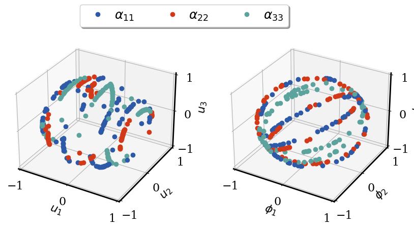
(b) Decomposition of self-combination after including contributions of the weights: ${\rm SVD}(\mathbf{W}^{T}_{q}\mathbf{W}_{k}\mathbf{y}_{j}\mathbf{y}^{T}_{i})$

(c) Decomposition of attention score: ${\rm SVD}\left(\rm{softmax}(\frac{\rm{Tr}(\mathbf{y}_{j}\mathbf{y}_{i}^{T}\mathbf{W}_{q}^{T}\mathbf{W}_{k})}{\sqrt{k}})\right)$

Figure 1: Three-dimensional scatter plots of left and right singular vectors ($u_{i}$ and $\phi_{i}$) of diagonal elements in the production matrices $\alpha$ of the inputs. The matrices are computed from (a) self-combination, (b) $\mathbf{K}\mathbf{Q}^{T}$ production and (c) attention score computed by $\rm softmax$, where $e$ denotes exponential. The diagonal elements are denoted by blue ($\alpha_{11}$), red ($\alpha_{22}$) and cyan ($\alpha_{33}$), respectively

The SVD of the combination matrix between $\mathbf{y}_{i}\mathbf{y}_{j}$, matrix product of query and key, and the attention score nonlinearised by $\rm softmax$ are shown in Fig. 1. Note that we only show the main diagonal elements of the $\bm{\alpha}$ matrix as these are the main contributors when computing the attention score. From the self-combination, one can observe that the space spanned by the left singular vectors, $\mathbf{u}$, has a somewhat cylindrical shape. However, the right singular vectors ${\bm{\phi}}$ exhibit a shape closer to that of a sphere. These shapes are connected with the unit circle, which is used to study unique sinusoidal functions. When analysing multiple waves with different phase shifts the unit circle is expected to grow in dimensions as the correlation matrix between input vectors increases. It can be claimed that as $r\rightarrow\infty$ for $\mathbf{Y}\in\mathbb{R}^{3\times r}$, the sphere would become denser, creating a fully compact surface; where $r$ is the rank of the matrix.

The eigenspaces for queries and keys, shown in Fig. 1(b), are observed to be fixed by rotations and translations of $\mathbf{W}_{q}^{T}\mathbf{W}_{k}$. These orbits constitute the subspace of the real domain, where the inner product exists. However, after the space compression forced by the trace and $\rm softmax$, this subdomain is reduced to a scalar, which is shown in Fig. 1(c) as a non-trivial space compression. One can interpret $\bm{\alpha}$ as the correlation between inputs of the transformer, such that $\alpha_{i,j}\in[0,1],\forall i,j$. In fact, the $\rm{softmax}$ is a probability distribution over three different possible trajectories, each trajectory being an input vector. For instance, the second element in the first row of $\bm{\alpha}$ is expressed as:

$$\alpha_{1,2}=\frac{e^{\frac{\rm{Tr}(\mathbf{y}_{j}\mathbf{y}_{i}^{T}\mathbf{W}_{q}^{T}\mathbf{W}_{k})}{\sqrt{k}}}}{\sum_{j=1}^{3}e^{\frac{\rm{Tr}(\mathbf{y}_{j}\mathbf{y}_{1}^{T}\mathbf{W}_{q}^{T}\mathbf{W}_{k})}{\sqrt{k}}}}.$$ (7)

In (7) it can be observed that the numerator ${e^{{\rm Tr}(\mathbf{W}_{q}^{T}\mathbf{W}_{k}\mathbf{y}_{2}\mathbf{y}_{1}^{T}})}=e^{\sum_{i=1}^{3}\lambda_{i}}$, and this is the correlation factor between $\mathbf{y}_{1}$ and $\mathbf{y}_{2}$; after dividing by all the correlations with $\mathbf{y}_{1}$, $\alpha_{1,2}$. Behaves like a probability distribution, when we later combine all possible trajectories spanned by $\mathbf{V(y_{j})}$ with their respective correlation factors, we obtain the expected trajectory as a reconstruction for the next time instances of the time series $\mathbf{y}_{1}$, expressed as $\mathbf{\hat{y}}_{1}$. Therefore $\mathbf{\hat{y}}_{i}=\mathbb{E}(X_{i})$ for a fixed $i$ where $i\in[1,3]$ and:

$$x_{j}\in X_{i};\quad x_{j}=\mathbf{W}_{V}\mathbf{y}_{j}(t);\quad p_{j}=\alpha_{i,j},$$ (8)

$$\mathbb{E}(X_{m})=\sum_{j=1}^{3}p_{j}x_{j}=\sum_{j=1}^{3}\alpha_{i,j}\mathbf{W}_{V}\mathbf{y}_{j}.$$ (9)

When computing the trace we compress all spatio-temporal correlations. In a continuous manner, this can be interpreted as a weighted integration over the past time. In conclusion, the $\bm{\alpha}$ matrix highlights the dependence between input vectors and all spatiotemporal reconstruction for $\mathbf{y}_{i}$ is performed by $\mathbf{W}_{V}\mathbf{y}_{i}$, as $\bm{\alpha}$ is a diagonal matrix due to the independence between wave phases, thus the prediction is expressed as:

$$\mathbf{\hat{y}}_{1}=\sum_{j=1}^{3}\alpha_{1,j}\mathbf{V(y_{j})}\approx\alpha_{1,1}\left(\sum_{k=1}^{3}\lambda_{k}\mathbf{v}_{k}c_{k,1}\right).$$ (10)

Based on the discussion above, the nature of the trace eliminates all backwards track-ability of the information, decreasing the relevance of the exact value of each matrix element. Therefore, it is reasonable to directly learn the exact $\bm{\alpha}$ value instead of learning the queries and keys matrices. Here we propose removing the $\mathbf{W}_{K}$, $\mathbf{W}_{Q}$ and $\rm softmax$ from the self attention, which also reduces the computational complexity of the problem from $4n_{i}^{2}$ to $2n_{i}^{2}$, where $n_{i}$ is the size for the input vectors, $\mathbf{y}_{i}(t)$.

At this stage, we employ the easy-attention module using an input of the same size as that of the self attention, and the same training setup for sinusoidal-waves reconstruction. Table 1 summarizes the obtained $l_{2}$-norm error, as well as computation time for training ($t_{c}$) and number of floating-point operations ($N_{f}$) of the employed easy-attention and self-attention modules. Note that we compute $N_{f}$ for one forward propagation using a batch size of 1. The results indicate that the easy attention reduces the complexity of self attention by 45% and saves computation time. The reconstruction results are shown in Fig. 2, where the superior performance of easy attention can be observed.

Name	Parameters	$\varepsilon$ (%)	$t_{c}$ (s)	$N_{f}$
Self-Attn	36	10%	26.88	81
Easy-Attn	18	0.0018%	19.20	45

Table 1: Summary of a single self-attention and a easy-attention module used for sinusoidal-waves reconstruction. In red we show the best reconstruction.

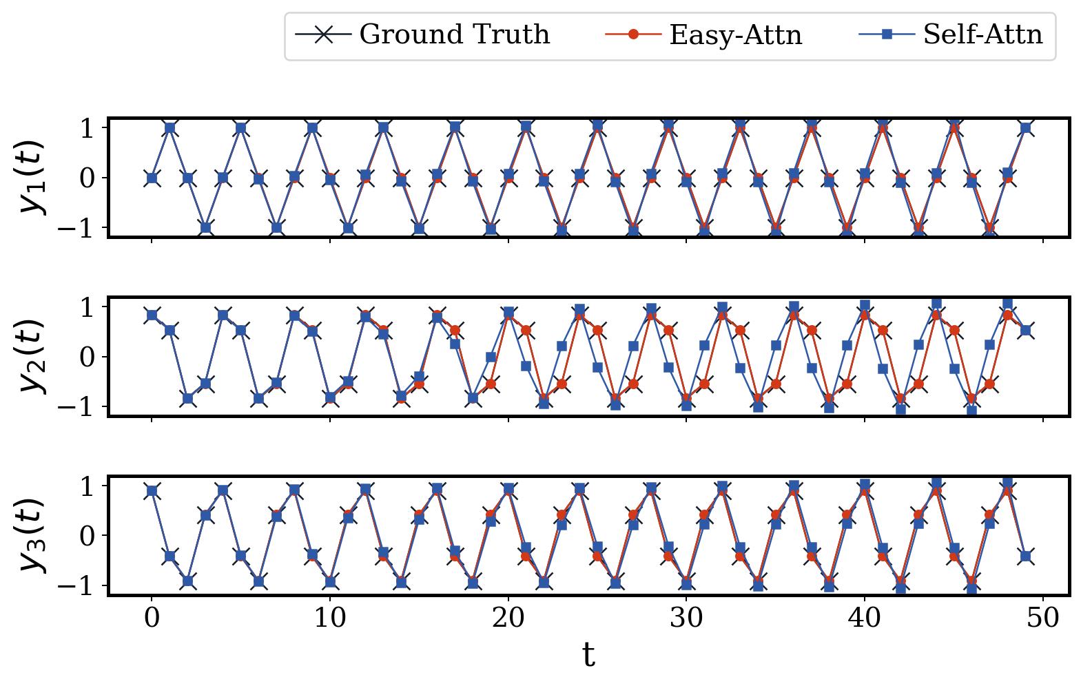
Figure 2: Reconstruction results of sine functions with phase shifts. Here we compare the ground truth with reconstructions through the self- and easy-attention methods.

Chaotic van der Pol oscillator with discrete Fourier transform

In this section, motivated by the promising reconstructing capability of the easy-attention module, the objective is to analyse the specific mechanism for both attention models searching for an explainability between input, output and learning parameters. Given the results discussed above, it can be observed that the easy attention exhibits promising performance on sinusoidal-wave reconstruction, which implies that the easy-attention method has the potential to take advantage of periodicity. This unique potential motivates us to study a more complex system through discrete Fourier transform, which produces the sinusoidal wave by implementing the Euler formula. To this end, we propose the method called multi-easy attention, which employs multiple easy-attention modules to learn the frequencies of the dominant $K$ amplitudes which are used to reconstruct the trajectory. In the present study, we determine the value of $K$ by requiring that the reconstructed trajectory must exhibit a reconstruction accuracy $E_{\rm rec}$ of 90%. We define the reconstruction accuracy as:

$$E_{\rm rec}=\left|1-\frac{||S-\tilde{S}||_{2}}{||S||_{2}}\right|\times 100\%,$$ (11)

where $S$ and $\tilde{S}$ denote original and reconstructed trajectories, respectively.

Fig. 3 illustrates the implementation of the multi-easy-attention method combined with the discrete Fourier transform. The trajectory is transformed into the frequency domain via the discrete Fourier transform, and we sort out the dominant $K$ amplitudes from all $M$ amplitudes. Subsequently, we employ $K$ attention modules to identify and reconstruct the frequencies in the form of the Euler formula. We utilize reconstructed frequencies from modules and their corresponding amplitudes to reconstruct the trajectory. Note that for each frequency we employ a single attention module with one head, and the the input size ($d_{\rm in}$) is equal to the smallest integer of the real part of its period ($P$), such that $d_{\rm in}\geq P$. If the period is infinity, we set $d_{\rm in}=2$. We employ SGD with learning rate of $1\times 10^{-3}$ as the optimizer and MSE as the loss function. Each module is trained for 1,000 epochs with batch size of 8. To investigate the difference between easy attention and self attention in terms of performance, we substitute the easy-attention module by self-attention to build a multi-self-attention method for reconstruction.

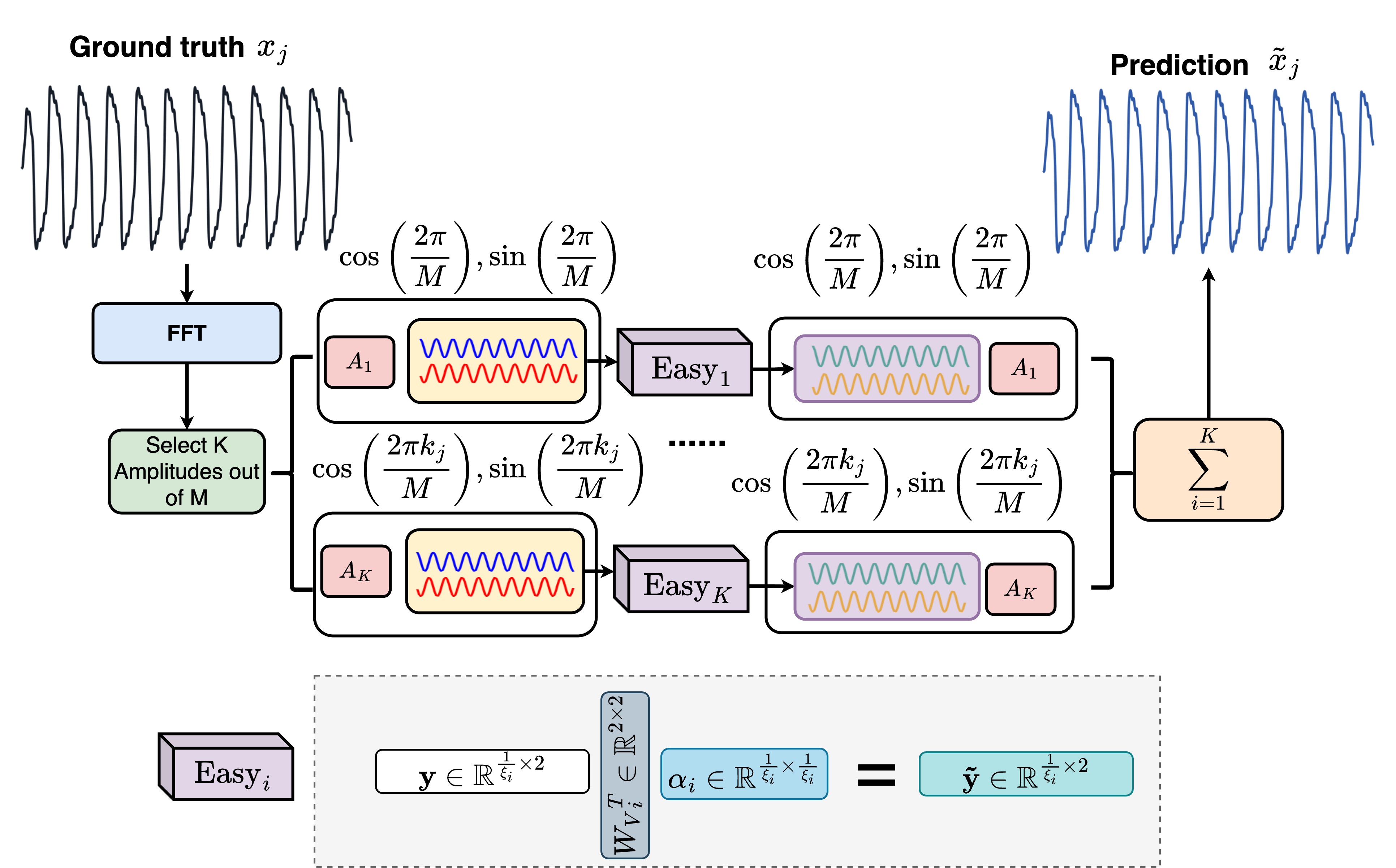
Figure 3: Schematic illustration of the multi-easy-attention method. We show the reconstruction of sinusoidal wave decomposed from discrete Fourier transform using the $K$ dominant amplitudes.

In the present study, we apply our method on the van der Pol chaotic system with a source term [38]:

$$\frac{{\rm d}x}{{\rm d}t}=y,\quad\frac{{\rm d}y}{{\rm d}t}=-x+a(1-x^{2})y+b\cos(\omega t),$$

where $a$, $b$ and $\omega$ are the parameters of the system. In the present study, we investigate three types of solutions, namely periodic $(a=5,b=40,\omega=7)$, quasi-periodic $(a=5,b=15,\omega=7)$ and chaotic $(a=5,b=3,\omega=1.788)$, which are discussed in Ref. [38]. Note that in the present study, we only investigate the temporal evolution of $x$ in the van der Pol system.

Table 2 lists the results of trajectory reconstruction multi-easy-attention and multi-self-attention, which are denoted as $\rm easy$ and $\rm self$, respectively. We compute the $l_{2}$-norm error as in Eq.(5) for each frequency and then average over the retained $K$ frequencies. The results demonstrate that easy attention significantly outperforms self-attention, as it is not only able to reconstruct all frequencies with a higher accuracy but also identifies differences in phase between the waves based on sine and cosine.

Case	K	$\overline{{\varepsilon}}_{\rm easy}$ (%)	$\overline{{\varepsilon}}_{\rm self}$ (%)
Periodic	100	0.149	92.517
Quasi-periodic	60	0.119	114.79
Chaotic	130	0.141	110.60

Table 2: Summary of $l_{2}$-norm error of prediction obtained by self-attention and easy-attention on the sinusoidal function of first $K$ amplitudes, where the best performance is colored in red. Note that the errors are calculated with respect to the Fourier-truncated signal.

To conclude this section, Table 2 demonstrates the capability of the multi-easy-attention to recognise and reconstruct dynamics. In Fig. 4 it can be observed that the easy attention replicates the dynamics of the original signal for all the studied sets of parameters, not only on the short term but as long as the period remains constant.

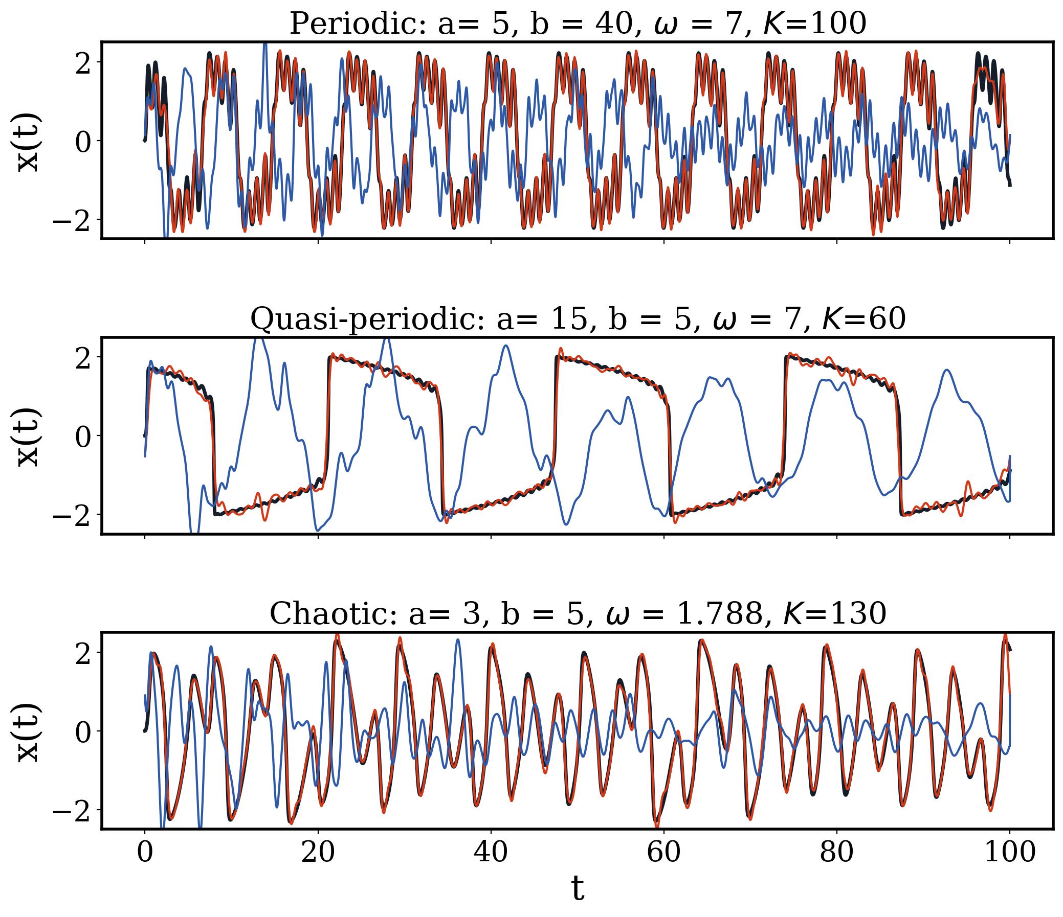
Figure 4: Reconstruction of temporal evolution of variable $x$ via sinusoidal wave decomposed from discrete Fourier transform using dominant $K$ amplitudes using varies models for three cases. In each subplot, the black line denotes the reference trajectory, whereas the red line and blue line denotes the reconstruction of multi-easy-attention and multi-self-attention, respectively.

Temporal dynamics predictions of Lorenz system using transformer with easy attention

To further examine the capabilities of the easy-attention method, we apply it on a transformer for temporal-dynamics prediction. We adopt the idea of time delay [4] for the task, which uses data sampled from the previous $p$ time steps to predict the next time one. A schematic illustration of the proposed transformer architecture is presented in Fig. 5. It comprises an embedding layer, a transformer encoder block and two decoding layer for time delay. Note that the multi-head attention in the encoder block is either easy attention or self attention in the present study. Instead of the positional encoding used in the original transformer, we adopt the sine time2vec embedding [39] to enhance identification of the temporal information present in the input sequence. The rectified linear unit (RELU) is employed as activation function for the feed-forward neural network. For the output encoding, the one-dimensional convolution neural network (Conv-1D) and multilayer perceptron (MLP) are employed to project the information as the prediction of the next time step. The employed transformer architectures are summarized in Table 3. Note that we apply dense and sparse multi-head easy attention as the easy attention module on the proposed architecture, respectively. The difference between the dense and sparse easy attention is that, for each head $i$, the dense easy attention learns all elements $\bm{\alpha}^{i}\in\mathbb{R}^{p\times p}$ while the sparse one only learns the main-diagonal elements of $\bm{\alpha}^{i}$.

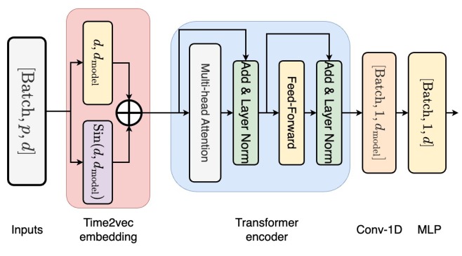
Figure 5: Schematic view of the transformer architecture for temporal-dynamics prediction. The dimension of the output for each layer has been indicated in each block, where the $p$ denotes the size of time delay whereas the $d$ and $d_{\rm model}$ denote the number of the features and the embedding size, respectively.

In addition, to investigate the difference in performance between easy-attention-based transformer and recurrent neural networks (RNNs), we also use the one-layer long short-term memory (LSTM) architecture. The LSTM model uses the same timebdelay $p$ as the transformer architectures with the number of units in the hidden layer being 128. We adopt Adam as the optimiser with a learning rate of $1\times 10^{-3}$, and the MSE loss function. The models are trained for 100 epochs with batch size of 32.

Name	$p$	$d_{\rm model}$	No.head	Feed-forward	No.Block
Easy-Attn	64	64	4	64	1
Sparse-Easy	64	64	4	64	1
Self-Attn	64	64	4	64	1

Table 3: Summary of transformer architecture employed in the Lorenz-system prediction. We denote the size of time delay as $p$ and the embedding size as $d_{\rm model}$, respectively. Note that the dense easy attention is denoted as Easy-Attn while the sparse easy attention is denoted as Sparse-Easy, respectively.

The Lorenz system [40] is governed by:

$$\frac{{\rm d}x}{{\rm d}t}=\sigma(y-x),\quad\frac{{\rm d}y}{{\rm d}t}=x(\rho-z)-y,\quad\frac{{\rm d}z}{{\rm d}t}=xy-\beta z,$$

where $x$, $y$, and $z$ are the state variables, whereas $\sigma$, $\rho$, and $\beta$ are the system parameters. We use the classical parameters of $\rho$ = 28, $\sigma$ = 10, $\beta$ = 8/3, which lead to chaotic behaviour. For this numerical example, we provide random initial conditions with $x_{0}$ $\sim$ $[-5,5]$, $y_{0}\sim[-5,5]$, $z_{0}\sim[0,5]$ to generate 100 time series for training and validation with a split ratio of 8:2. Each time series contains 10,000 time steps with a time-step size of $\Delta t$ = 0.01 solved using a Runge–Kutta numerical solver. The test data is generated by integrating the system with new initial states of $x_{0}=y_{0}=z_{0}=6$ with independent perturbations $\epsilon_{x}$, $\epsilon_{y}$ and $\epsilon_{z}$ where $\epsilon_{i}\sim\mathcal{N}(0,1)$ (note that $\mathcal{N}(0,1)$ denotes a normal distribution with 0 average and a standard deviation of 1) for each variable. We adopt the same time-step size and number of time steps of 10,000 to generate 1 time series as test data. We employ the relative $l_{2}$-norm error $\varepsilon$ to assess the prediction accuracy, which is expressed as:

$$\varepsilon=\frac{||\mathbf{u}_{\rm pred}-\mathbf{u}_{\rm sol}||_{2}}{||\mathbf{u}_{\rm sol}||_{2}}\times 100\%,$$ (12)

where $\mathbf{u}_{\rm pred}$ and $\mathbf{u}_{\rm sol}$ are the model prediction and the solution from numerical solver, respectively. Following the assessment in Ref. [30], we evaluate the error of each variable obtained by proposed models at time-step over 512 time steps on the test dataset. We also assess the computation time of training ($t_{c}$) and number of floating-point operations ($N_{f}$) for one forward propagation with batch size of 1.

We summarise the results in Table 4, where the proposed model using dense easy attention achieves the lowest error, 1.99%, demonstrating the superior performance of the easy-attention method applied on temporal-dynamics predictions. The LSTM model has the highest number of learnable parameters, but the lowest training time and number of floating-point operations. However, it yields the highest $l_{2}$-norm error of 37.68%, which indicates that the LSTM model is not able to reproduce the correct dynamical behaviour over long time. The dense-easy-attention model reduces the time for training by 17% and the computational complexity by 25% of the self-attention-based model while surpassing the number of learnable parameters of the self-attention-based model. This is due to the fact that the dense-easy-attention module comprises $\bm{\alpha}\in\mathbb{R}^{h\times p\times p}$ and $\mathbf{W}_{V}\in\mathbb{R}^{p\times d_{\rm model}}$ while the self-attention module comprises $\mathbf{W}_{Q},\mathbf{W}_{K},\mathbf{W}_{V},\mathbf{W}_{C}\in\mathbb{R}^{p\times d_{\rm model}}$ which has fewer parameters in the present study. However the computational cost for the easy-attention models is lower than the self-attention since the softmax and the inner product inside the latter are eliminated. Note that the model employing sparse easy attention exhibits an error of 2.79% while only having 52% of the learnable parameters of the self-attention-based transformer, which implies that the sparsification benefits the robustness of the easy-attention method applied to temporal-dynamics prediction.

Name	Parameters	$\varepsilon$ (%)	$t_{c}$ (s)	$N_{f}$
Easy-Attn	29.75 $\times$ $10^{3}$	1.99	9.16 $\times$ $10^{3}$	49.22 $\times$ $10^{3}$
Sparse-Easy	13.44 $\times$ $10^{3}$	2.79	9.10 $\times$ $10^{3}$	49.22 $\times$ $10^{3}$
Self-Attn	25.48 $\times$ $10^{3}$	7.36	11.07 $\times$ $10^{3}$	65.61 $\times$ $10^{3}$
LSTM	37.51 $\times$ $10^{3}$	37.68	4.85 $\times$ $10^{3}$	41.00 $\times$ $10^{3}$

Table 4: Summary of results on the Lorenz system obtained from different models. In red we show the lowest prediction error.

The long-term predictions of the variables over 10,000 time steps are shown in Fig. 6 for various models on the test dataset. The results clearly show that the LSTM and self-attention-based transformer model are not able to reproduce the correct dynamical behaviour over long times, while the transformer models using easy attention are able to achieve better predictions; this can be clearly observed in the temporal evolution of variable $x$ from the Lorenz system, shown in Fig. 7. Compared with the self-attention-based transformer, the transformers using easy attention have the lowest computational cost for training and exhibit higher accuracy on reproduction of long-term dynamics, which indicates that the transformer models using easy attention are more robust for temporal-dynamics prediction than the model using self attention.

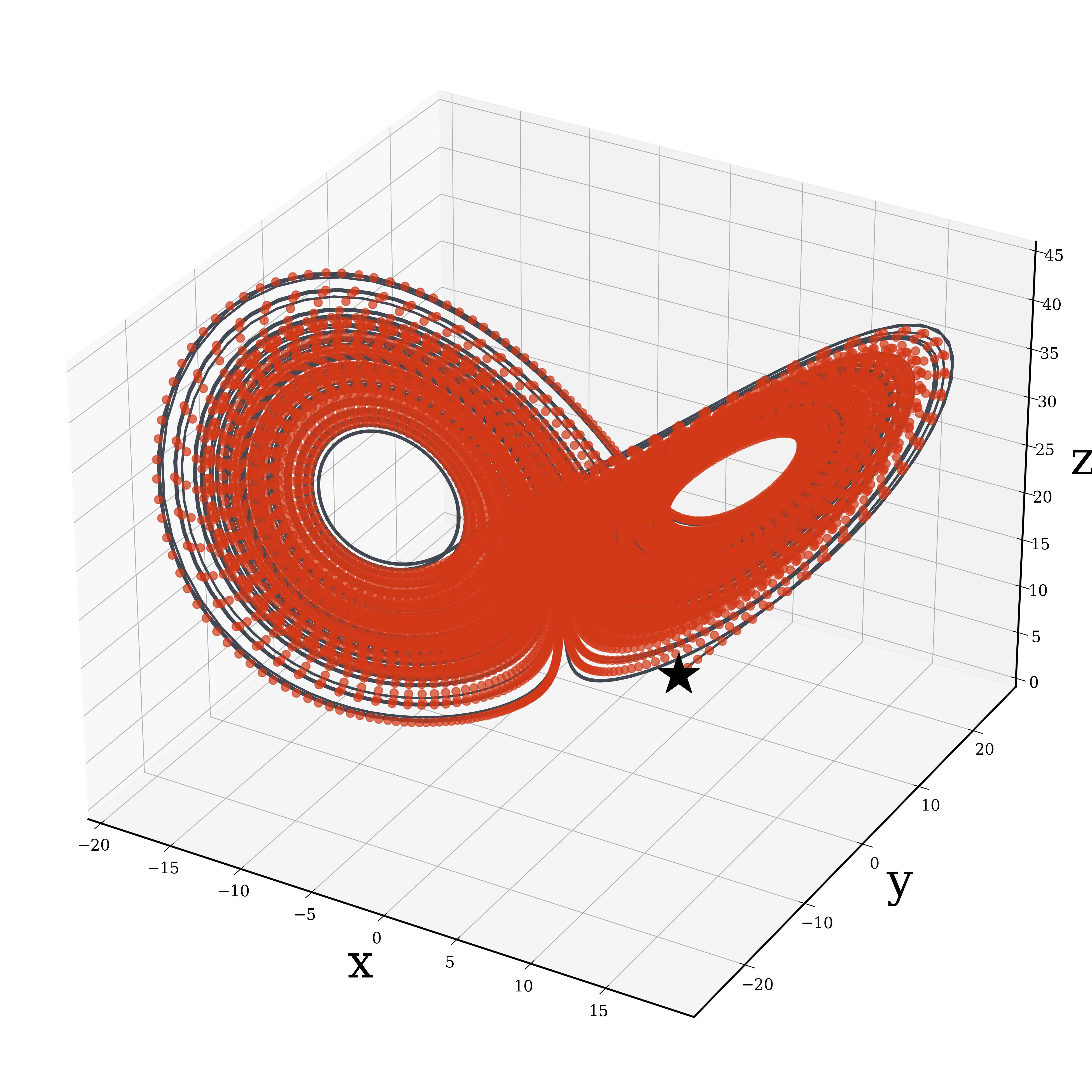
(a) Easy attention

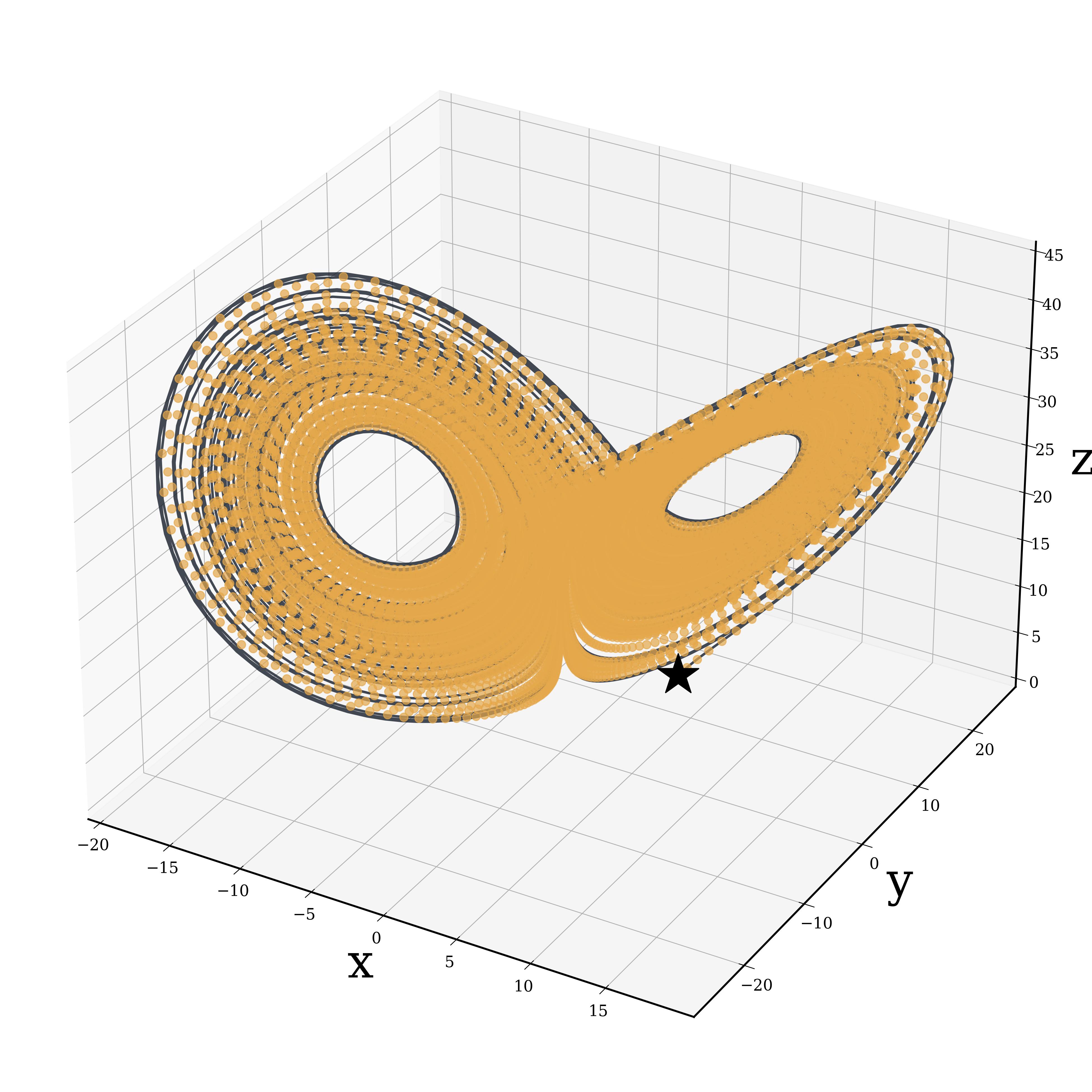
(b) Sparse easy attention

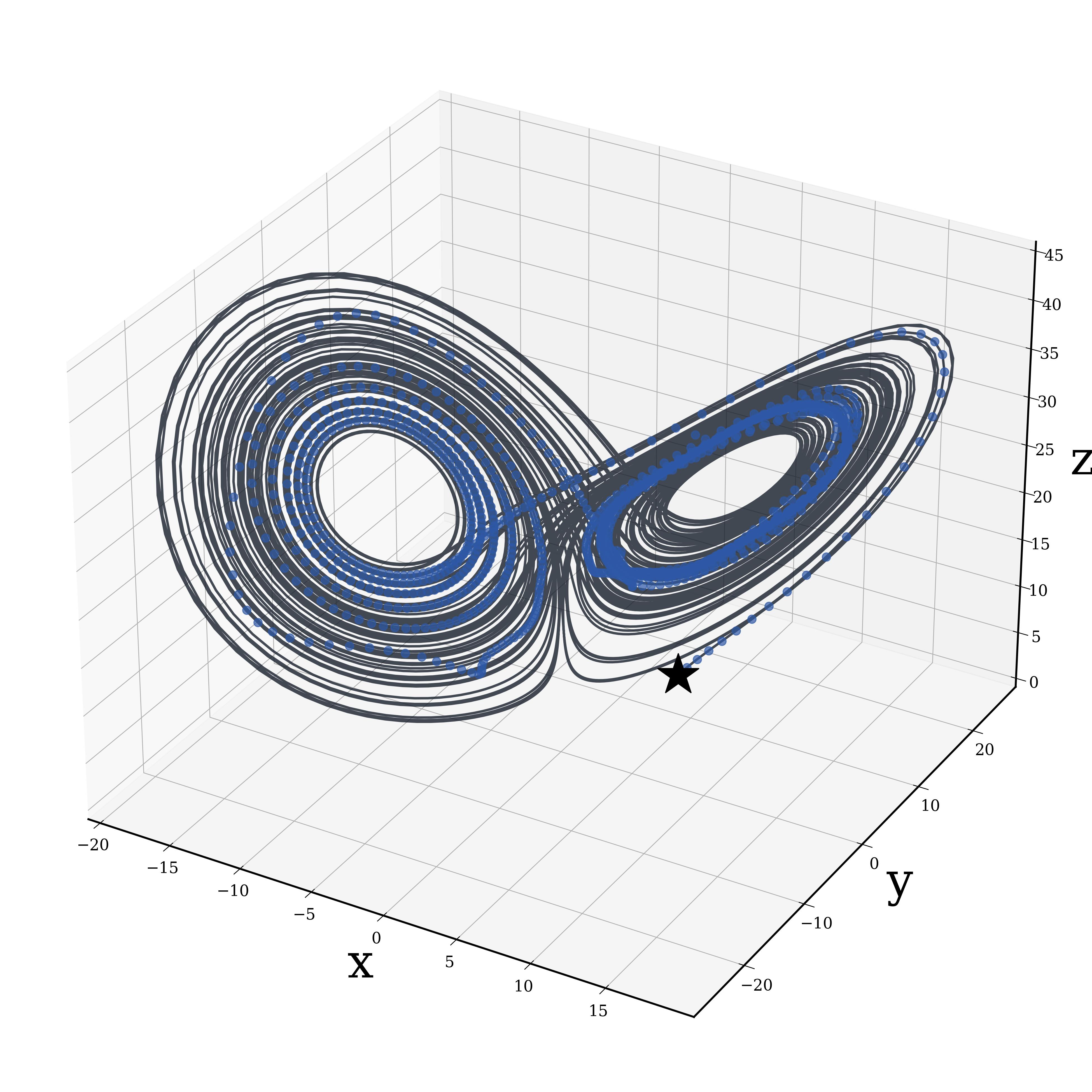
(c) Self attention

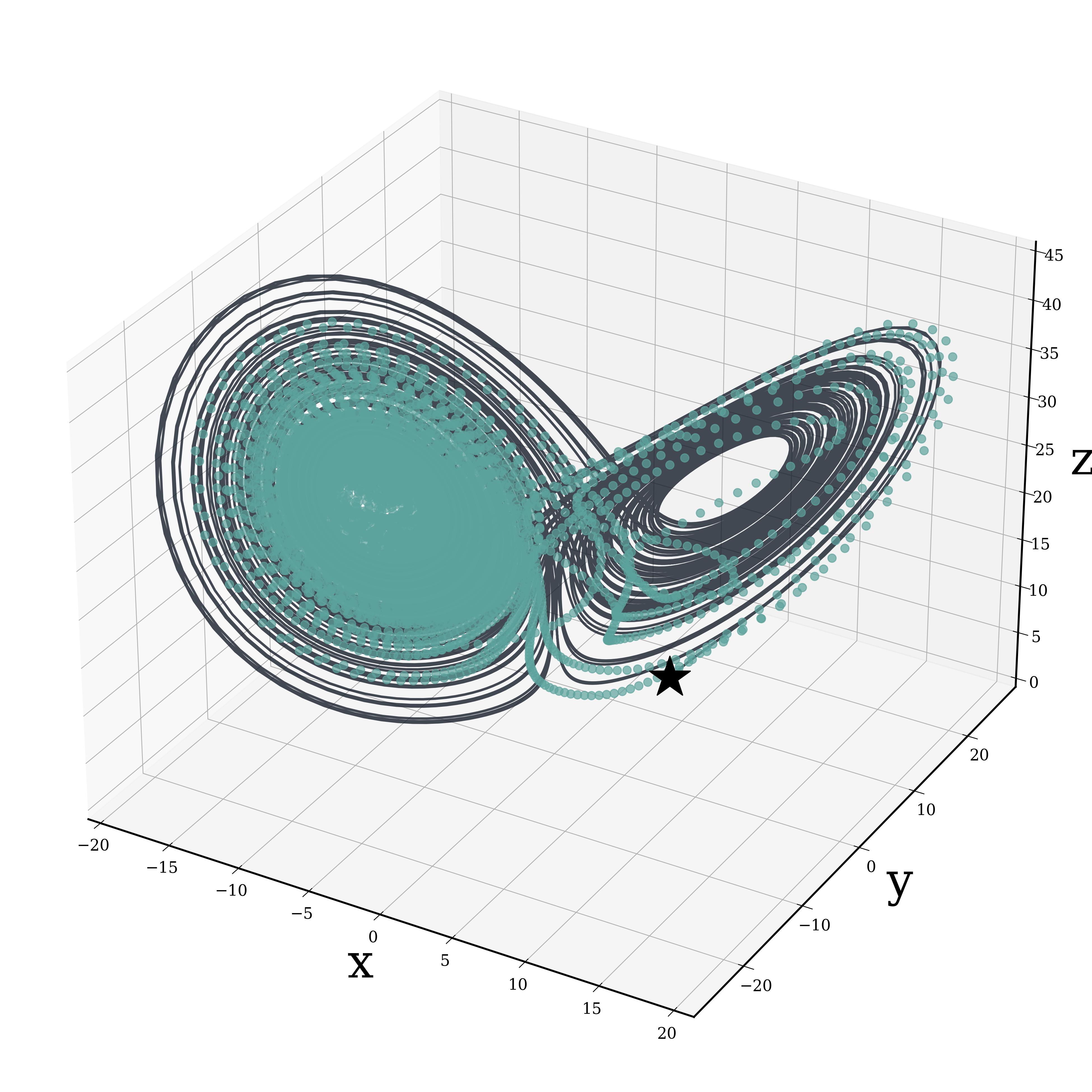
(d) LSTM

Figure 6: Visualisation of Lorenz system predicted by the different models. The test data is generated by integrating the system with new initial states of $x_{0}=y_{0}=z_{0}=6$ with independent perturbations $\epsilon_{x}$, $\epsilon_{y}$ and $\epsilon_{z}$ where $\epsilon_{i}\sim\mathcal{N}(0,1)$ for each variable. Note that the test data is indicated in black as reference and the location of initial condition ($x_{0}$, $y_{0}$, $z_{0}$) is marked as a black star.

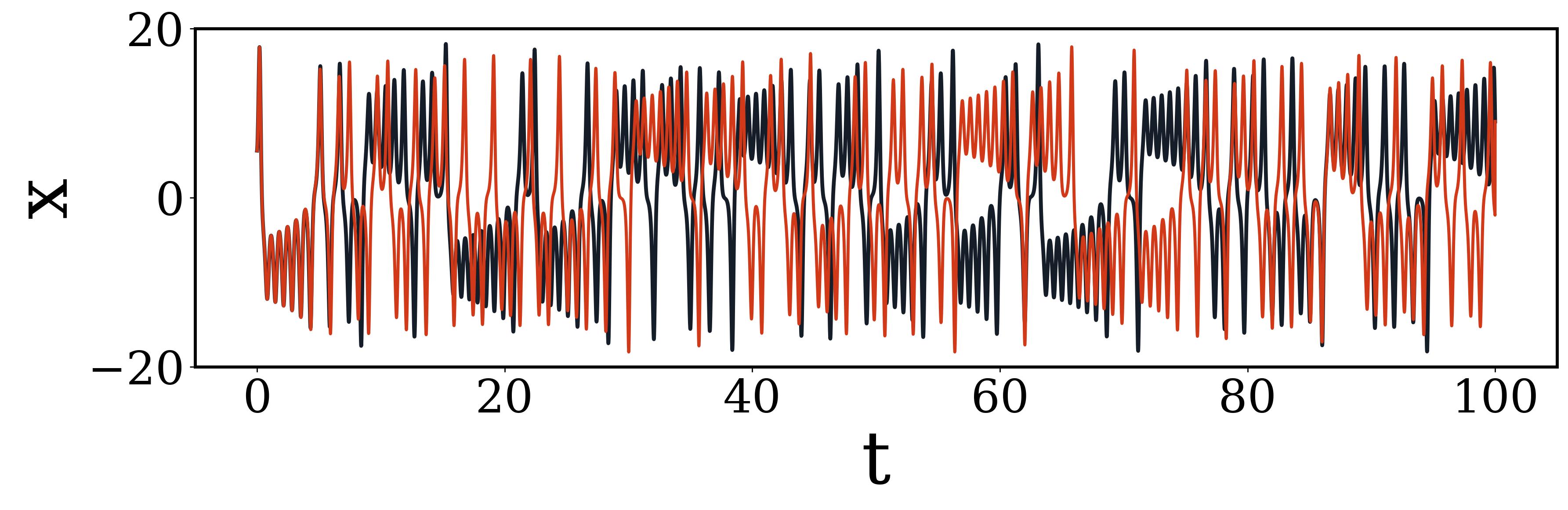
(a) Easy attention

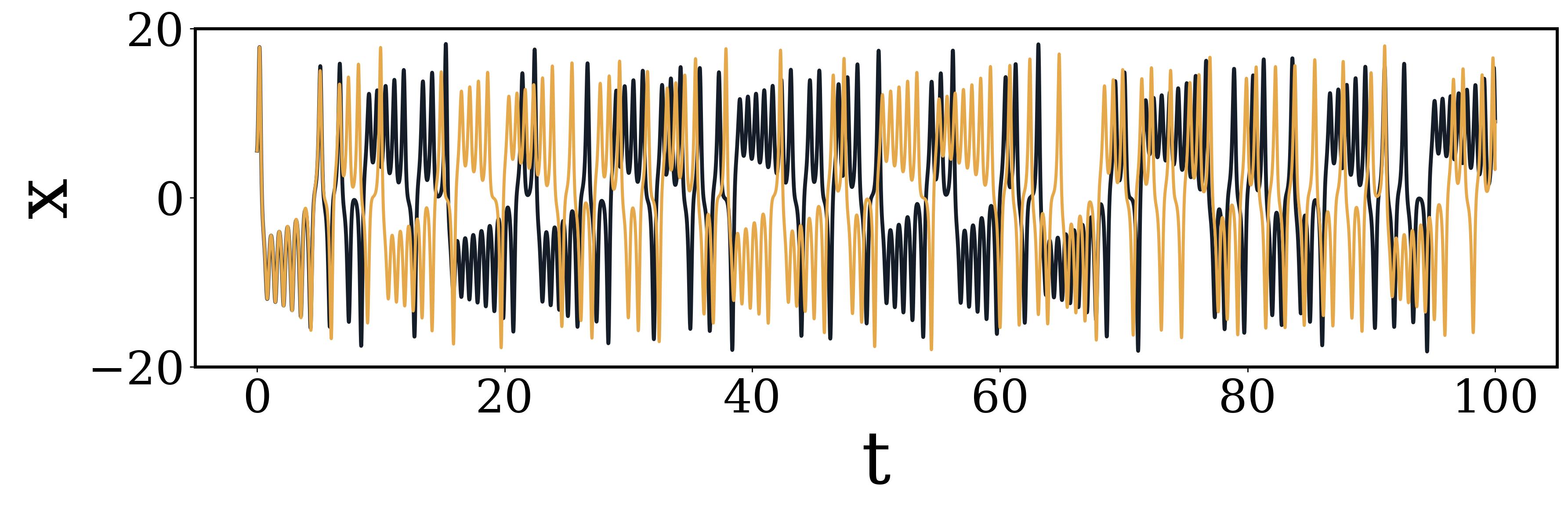
(b) Sparse easy attention

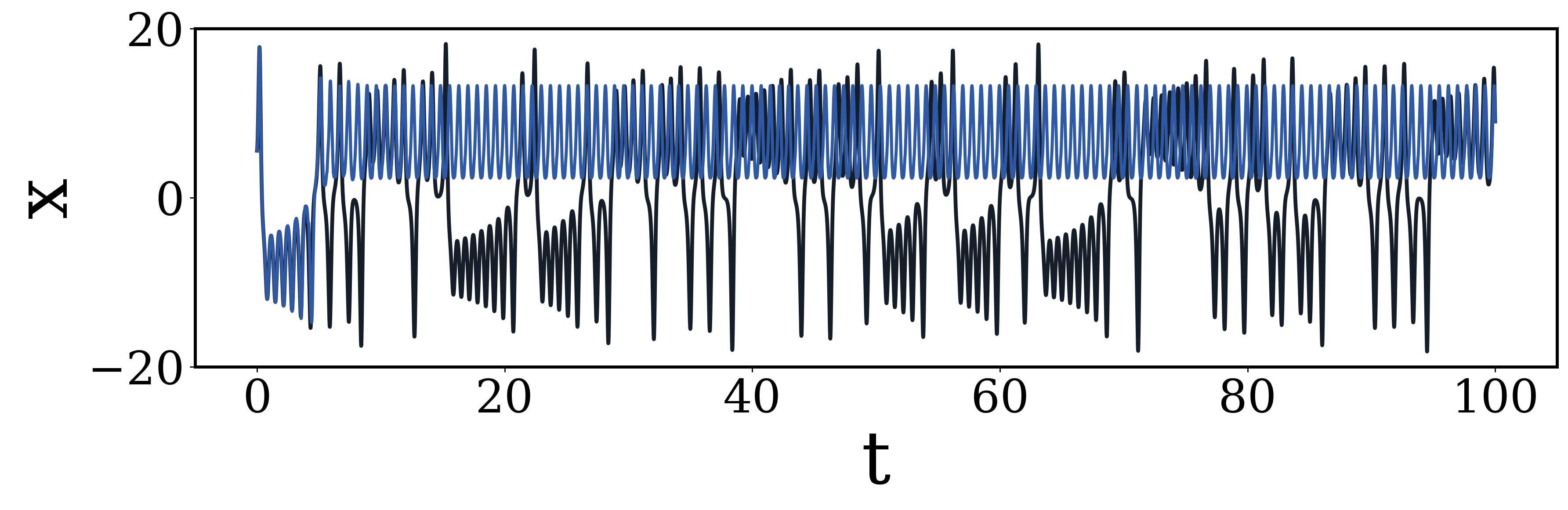
(c) Self attention

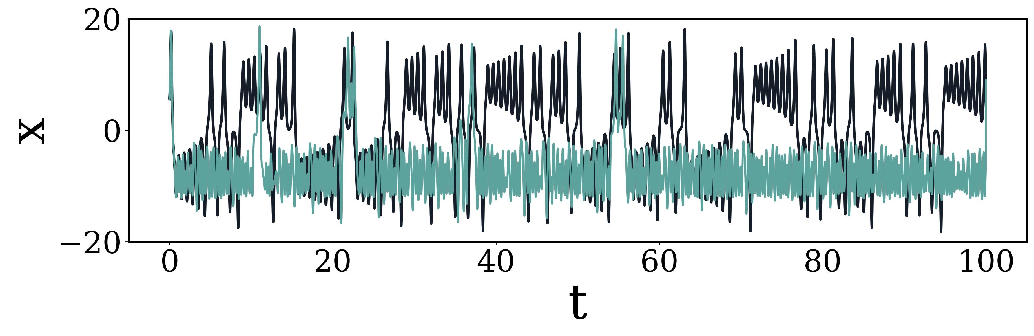
(d) LSTM

Figure 7: Temporal evolution of variable $x$ from the Lorenz system predicted by the different models. The test data is generated by integrating the system with new initial states of $x_{0}=y_{0}=z_{0}=6$ with independent perturbations $\epsilon_{x}$, $\epsilon_{y}$ and $\epsilon_{z}$ where $\epsilon_{i}\sim\mathcal{N}(0,1)$ for each variable. Note that the test data is indicated in black as reference.

Summary and conclusions

In the present study we proposed a novel attention mechanism for transformer neural networks, namely easy attention, which does not rely on queries and keys to generate attention scores and removes the nonlinear $\rm softmax$ function away. The easy attention arises from the nonelastic nature of the trace, as this makes impossible any backwards track-ability of the information, decreasing the relevance of the exact value of each matrix element. Taking this into account, we proposed to learn the attention scores $\bm{\alpha}$ instead of learning the queries and keys matrices, removing the $\mathbf{W}_{K}$, $\mathbf{W}_{Q}$ and $\rm softmax$ from the self attention, yielding a considerable reduction in the numbers of parameters. Furthermore, we propose the sparse easy attention, which reduces the number of learnable parameters of the tensor $\bm{\alpha}$ by only learning the diagonal elements, and a method to perform multi-head easy attention which employs multiple $\bm{\alpha}$ to improve the long-term predictions.

We start with sinusoidal functions and we investigate the core idea of self attention by implementing SVD on the $\mathbf{K}\mathbf{Q}^{T}$ product and the $\rm softmax$ attention score. The results reveal that the self attention in fact compresses the input sequence self-combination eigenspace. Following this observation, we propose our easy-attention mechanism. For sinusoidal-wave reconstruction, the easy-attention model achieves 0.0018% $l_{2}$-norm error with less computation time for training and complexity than self attention, which exhibits $l_{2}$-norm error of 10%. Motivated by the promising performance on sinusoidal-wave reconstruction, we propose the multi-easy-attention method, which combines the discrete Fourier transform with attention mechanism for signal reconstruction. We apply our method on the Van der Pol oscillator for three cases: periodic, quasi-periodic and chaotic [38]. The multi-easy-attention method can effectively reconstruct 90% of the reconstructed accuracy $E_{\rm{rec}}$ in all the cases, significantly outperforming the self attention. The unique capability of easy attention to learn long-term dynamics for periodic signals suggests that it may have a great potential for additional applications, such as signal de-noising.

Subsequently, we apply easy attention in the proposed transformer model for temporal-dynamics prediction of chaotic systems and we investigate the performance of our models on the Lorenz system. The transformer model with dense easy attention yields the lowest relative $l_{2}$-norm error of 2.0%, outperforming the same transformer architecture with the self attention (7.4%) and the LSTM model (37.7%). The results also show that, compared with self-attention-based transformer, the transformers using easy attention have a much lower computational cost and exhibit less complexity. Thus the transformer model using easy attention is more robust for temporal-dynamics predictions.

In conclusion, the easy-attention mechanism, due to its robustness, exhibits promising performance in the tasks of signal/trajectory reconstruction as well as temporal-dynamics prediction in low-dimensional chaotic systems. Our results also indicate potential for application in more complex large-scale dynamical systems, since transformer networks are naturally designed for high-dimensional sequence data [25, 30, 31, 32, 33],

Methods

Here, we will focus on the mathematical development of the easy-attention method and its implications on the final output. To this end we will first examine the self-attention model. The mathematical implementation of a transformer encoder block is expressed as follows [41]. First, a transformer block is a parameterised function $T:\mathbb{R}^{n\times d}\rightarrow\mathbb{R}^{n\times d}$. If $x\in\mathbb{R}^{n\times d}\Rightarrow T(x)=\hat{x}$, where:

$$\mathbf{Q}(\mathbf{x}_{i})=\mathbf{W}_{q}\mathbf{x}_{i},\quad\mathbf{K}(\mathbf{x}_{i})=\mathbf{W}_{k}\mathbf{x}_{i},\quad\mathbf{V}(\mathbf{x}_{i})=\mathbf{W}_{v}\mathbf{x}_{i};\quad\mathbf{W}_{q},\mathbf{W}_{k},\mathbf{W}_{v}\in\mathbb{R}^{d\times k}.$$ (13)

The so-called queries, keys and values are constructed based on three different independent weight matrices $\mathbf{W}_{q}$, $\mathbf{W}_{k}$, $\mathbf{W}_{v}$, which are all learned during training. It is important to remark that these weight matrices do not converge and are not unique. The attention score $\alpha_{i,j}$ is computed as:

$$\alpha_{i,j}={{\rm softmax}_{j}}\left(\frac{\langle\;\mathbf{Q}^{T}(\mathbf{x}_{i}),\mathbf{K}^{T}(\mathbf{x}_{j})\rangle}{{\sqrt{k}}}\right);\quad{\rm softmax}(z)=\frac{{\rm exp}(z)}{\sum_{k=1}^{m}{\rm exp}(z)_{k}}.$$ (14)

The well-known $\rm softmax$ is a generalization of the logistic function used for compressing $d$-dimensional vectors of arbitrary real entries to real vectors of the same dimension in the range $[0,1]$, which is expressed as:

$$\mathbf{\hat{x}}_{i}=\mathbf{W}_{c}\sum_{j=1}^{n}\alpha_{i,j}\mathbf{V}(\mathbf{x}_{j})=\mathbf{W}_{c}\sum_{j=1}^{n}\alpha_{i,j}\left(\sum_{k=1}^{n}\lambda_{k}\mathbf{v}_{k}c_{k,j}\right).$$ (15)

One can represent the product $\mathbf{W}_{v}\mathbf{x}_{i}$ as a linear combination of the eigenvectors and eigenvalues ($\mathbf{v}_{k},\lambda_{k}$) of $\mathbf{W}_{V}$ for unique coefficients $c_{k,j}$. For analytical purposes we will express the inner product inside the $\rm softmax$ operation in terms of the trace so one can take advantage of its cyclic property:

$$\alpha_{i,j}={\rm softmax}\left(\frac{\rm{Tr}(\mathbf{W}_{q}^{T}\mathbf{W}_{k}\mathbf{x}_{j}\mathbf{x}_{i}^{T})}{\sqrt{k}}\right).$$ (16)

In this study we asses the importance of the weight matrices for the accuracy of the predictions and note that the result depends on eigenvalues of $\mathbf{W}_{k}^{T}\mathbf{W}_{q}\mathbf{x}_{i}\mathbf{x}_{j}^{T}$. Given the nature of the trace, introduced on the interpretation of the attention mechanism, the transformer only uses the final result of the sum. For example: ${\rm Tr}(Z)=a+b+c=d$, where $a,b,c,d\in\mathbb{R}$, and in principle there are infinite possible values of $a$, $b$, $c$ such that the sum is equal to $d$. Based on this, we propose a simplified attention mechanism which we denote easy attention, defined as:

$$\mathbf{\hat{x}}_{i}=\sum^{n}_{j=1}\alpha_{i,j}{\mathbf{W}_{V}}\mathbf{x}_{j}.$$ (17)

In this way, the keys and queries in self attention are eliminated. We directly learn $\bm{\alpha}$ as a learnable attention-score tensor of the spanned eigenspace of the self-combination time-delay input matrix. As consequence, only $\bm{\alpha}$ and $\mathbf{W}_{V}$ are required to learn in easy attention. In particular, an input tensor $\mathbf{x}$ is projected as the value tensor $\mathbf{V}$ by $\mathbf{W}_{V}$. Subsequently, we compute the product of $\mathbf{V}$ and the attention scores $\alpha_{i,j}$ as the output $\mathbf{\hat{x}}_{i}$.

Furthermore, $\bm{\alpha}$ can be sparsified by learning the diagonal elements only, or with elements distributed in off-diagonal positions both above and below the main diagonal if necessary, which further reduces the number of learnable parameters of the easy-attention mechanism. At the stage of forward propagation or inference, those parameters are assigned to the corresponding indices in a matrix of dimension $\mathbb{R}^{n\times n}$. Fig. 8(a) illustrates the difference between the dense and sparse easy-attention methods. In the present study, we only consider learning main-diagonal elements as sparsifiaction.

Apart from defining a single easy-attention function with one learnable attention-score tensor $\bm{\alpha}$ as in (17), it is possible to employ multiple $\bm{\alpha}$ tensors to implement the so-called multi-head easy attention, following an idea similar to that of self attention [26], which is defined as:

$$\begin{split}\mathbf{\hat{x}}=\rm{concat}\{\mathbf{\tilde{x}}_{i}\}_{i=1}^{h};\quad\mathbf{\tilde{x}}_{i}\in\mathbb{R}^{n\times k},\\ \mathbf{\tilde{x}}_{i}=\sum_{j=1}^{n}\alpha^{i}_{i,j}\mathbf{W}^{i}_{V}\mathbf{x}_{j},\end{split}$$ (18)

where $h$ denotes the number of heads and $i\in[0\sim h]$, as we split $\mathbf{W}_{V}$ into $h$ matrices one for each $\mathbf{\tilde{x}}_{i}\in\mathbb{R}^{n\times k}$. The prediction $\mathbf{\hat{x}}$ for the multi-head easy attention is a concatenation of $\mathbf{\tilde{x}}_{i}$. Note that the difference between multi-head self attention and multi-head easy attention is that, in the latter, we do not employ another linear layer for projecting the concatenated sequence, which further reduces the complexity. The multi-head easy attention is beneficial to preserve long-term dependencies when $d$ becomes large. The mechanism of single and multi-head easy attention are illustrated in Fig. 8.

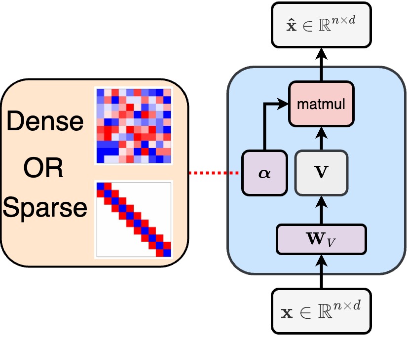
(a) Single easy attention

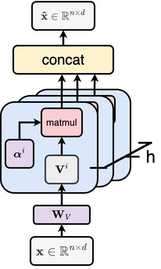
(b) Multi-head easy attention

Figure 8: Schematic view of single easy-attention mechanism (left) and multi-head easy attention (right). Note that the trainable weight tensors $\mathbf{W}_{V}$ and $\bm{{\alpha}}$ are denoted by purple blocks. The difference between the dense and sparse easy-attention methods is illustrated in the orange block. The $\rm matmul$ in the red block and the $\rm concat$ in the yellow block denote the matrix-product operator and tensor concatenation, respectively.

In the present study, all the model training and testing are implemented on a single central-processing unit (CPU) from a machine with the following characteristics: AMD Ryzen 9 7950X with 16 cores, 32 threads, 4.5 Ghz and 62 GB RAM. All machine-learning models and experiments were conducted using the PyTorch framework [42] (version 2.0.0). PyTorch was chosen due to its flexibility, ease of use, and extensive support for deep learning research. The custom models and neural-network architectures used in this work were implemented using PyTorch’s modular design, allowing seamless composition of layers and custom components. All the data and codes will be made available open access upon publication of the manuscript in the following repository: https://github.com/KTH-FlowAI

References

References

- Takens [1981] F. Takens, Detecting strange attractors in turbulence, in Dynamical Systems and Turbulence, Warwick 1980, edited by D. Rand and L.-S. Young (Springer Berlin Heidelberg, Berlin, Heidelberg, 1981) pp. 366–381.
- Mezić and Banaszuk [2004] I. Mezić and A. Banaszuk, Comparison of systems with complex behavior, Physica D: Nonlinear Phenomena 197, 101 (2004).
- Arbabi and Mezić [2017] H. Arbabi and I. Mezić, Ergodic theory, dynamic mode decomposition, and computation of spectral properties of the koopman operator, SIAM Journal on Applied Dynamical Systems 16, 2096 (2017).
- Pan and Duraisamy [2020a] S. Pan and K. Duraisamy, On the structure of time-delay embedding in linear models of non-linear dynamical systems, Chaos: An Interdisciplinary Journal of Nonlinear Science 30, 073135 (2020a).
- Lumley [1967] J. Lumley, The structure of inhomogeneous turbulent flows, Atmospheric turbulence and radio wave propagation 23, 166 (1967).
- Towne et al. [2018] A. Towne, O. T. Schmidt, and T. Colonius, Spectral proper orthogonal decomposition and its relationship to dynamic mode decomposition and resolvent analysis, Vol. 847 (2018) pp. 821–867.
- Schmid [2010] P. J. Schmid, Dynamic mode decomposition of numerical and experimental data, Journal of Fluid Mechanics 656, 5–28 (2010).
- Le Clainche and Vega [2017] S. Le Clainche and J. M. Vega, Higher order dynamic mode decomposition, SIAM Journal on Applied Dynamical Systems 16, 882 (2017).
- Mezić [2005] I. Mezić, Spectral properties of dynamical systems, model reduction and decompositions, Nonlinear Dynamics 41, 309 (2005).
- Koopman and Neumann [1932] B. O. Koopman and J. v. Neumann, Dynamical systems of continuous spectra, Proceedings of the National Academy of Sciences 18, 255 (1932).
- Pan and Duraisamy [2020b] S. Pan and K. Duraisamy, Physics-informed probabilistic learning of linear embeddings of nonlinear dynamics with guaranteed stability, SIAM Journal on Applied Dynamical Systems 19, 480–509 (2020b).
- Rowley et al. [2009] C. W. Rowley, I. Mezić, S. Bagheri, P. Schlatter, and D. S. Henningson, Spectral analysis of nonlinear flows, Journal of Fluid Mechanics 641, 115–127 (2009).
- Lusch et al. [2018] B. Lusch, J. N. Kutz, and S. L. Brunton, Deep learning for universal linear embeddings of nonlinear dynamics, Nature communications 9, 4950 (2018).
- Khodkar et al. [2019] M. A. Khodkar, P. Hassanzadeh, and A. Antoulas, A Koopman-based framework for forecasting the spatiotemporal evolution of chaotic dynamics with nonlinearities modeled as exogenous forcings (2019), arXiv:1909.00076 .
- Bevanda et al. [2021] P. Bevanda, S. Sosnowski, and S. Hirche, Koopman operator dynamical models: Learning, analysis and control, Annual Reviews in Control 52, 197 (2021).
- Eivazi et al. [2021] H. Eivazi, L. Guastoni, P. Schlatter, H. Azizpour, and R. Vinuesa, Recurrent neural networks and Koopman-based frameworks for temporal predictions in a low-order model of turbulence, International Journal of Heat and Fluid Flow 90, 108816 (2021).
- Box and Jenkins [2008] G. Box and G. M. Jenkins, Time series analysis forecasting and control, 4th ed. (Wiley, 2008).
- Goodfellow et al. [2016] I. Goodfellow, Y. Bengio, and A. Courville, Deep learning (MIT Press, 2016).
- Hochreiter and Schmidhuber [1997] S. Hochreiter and J. Schmidhuber, Long short-term memory, Neural Computation 9, 1735 (1997).
- Hasegawa et al. [2020] K. Hasegawa, K. Fukami, T. Murata, and K. Fukagata, Machine-learning-based reduced-order modeling for unsteady flows around bluff bodies of various shapes, Theoretical and Computational Fluid Dynamics 34, 367 (2020).
- Srinivasan et al. [2019] P. A. Srinivasan, L. Guastoni, H. Azizpour, P. Schlatter, and R. Vinuesa, Predictions of turbulent shear flows using deep neural networks, Physical Review Fluids 4, 054603 (2019).
- Wan et al. [2019] R. Wan, S. Mei, J. Wang, M. Liu, and F. Yang, Multivariate temporal convolutional network: A deep neural networks approach for multivariate time series forecasting, Electronics 8, 876 (2019).
- Bai et al. [2018] S. Bai, J. Z. Kolter, and V. Koltun, An empirical evaluation of generic convolutional and recurrent networks for sequence modeling (2018), arXiv:1803.01271 .
- Gan et al. [2021] Z. Gan, C. Li, J. Zhou, and G. Tang, Temporal convolutional networks interval prediction model for wind speed forecasting, Electric Power Systems Research 191, 106865 (2021).
- Wu et al. [2022] P. Wu, F. Qiu, W. Feng, F. Fang, and C. Pain, A non-intrusive reduced order model with transformer neural network and its application, Physics of Fluids 34, 115130 (2022).
- Vaswani et al. [2017] A. Vaswani, N. Shazeer, N. Parmar, J. Uszkoreit, L. Jones, A. N. Gomez, L. Kaiser, and I. Polosukhin, Attention is all you need, in Advances in Neural Information Processing Systems, Vol. 30, edited by I. Guyon, U. V. Luxburg, S. Bengio, H. Wallach, R. Fergus, S. Vishwanathan, and R. Garnett (2017).
- Gillioz et al. [2020] A. Gillioz, J. Casas, E. Mugellini, and O. A. Khaled, Overview of the transformer-based models for NLP tasks, in 2020 15th Conference on Computer Science and Information Systems (FedCSIS) (2020) pp. 179–183.
- Han et al. [2023] K. Han, Y. Wang, H. Chen, X. Chen, J. Guo, Z. Liu, Y. Tang, A. Xiao, C. Xu, Y. Xu, Z. Yang, Y. Zhang, and D. Tao, A survey on vision transformer, IEEE Transactions on Pattern Analysis and Machine Intelligence 45, 87 (2023).
- Yousif et al. [2023] M. Z. Yousif, M. Zhang, L. Yu, R. Vinuesa, and H. Lim, A transformer-based synthetic-inflow generator for spatially developing turbulent boundary layers, Journal of Fluid Mechanics 957, A6 (2023).
- Geneva and Zabaras [2022] N. Geneva and N. Zabaras, Transformers for modeling physical systems, Neural Networks 146, 272 (2022).
- Solera-Rico et al. [2023] A. Solera-Rico, C. S. Vila, M. Gómez, Y. Wang, A. Almashjary, S. Dawson, and R. Vinuesa, -variational autoencoders and transformers for reduced-order modelling of fluid flows, arXiv preprint arXiv:2304.03571 (2023).
- Cao [2021] S. Cao, Choose a transformer: Fourier or Galerkin, in Advances in Neural Information Processing Systems, Vol. 34, edited by M. Ranzato, A. Beygelzimer, Y. Dauphin, P. Liang, and J. W. Vaughan (Curran Associates, Inc., 2021) pp. 24924–24940.
- Katharopoulos et al. [2020] A. Katharopoulos, A. Vyas, N. Pappas, and F. Fleuret, Transformers are RNNs: Fast autoregressive transformers with linear attention (2020) pp. 5156–5165.
- Kitaev et al. [2020] N. Kitaev, Łukasz Kaiser, and A. Levskaya, Reformer: The efficient transformer (2020), arXiv:2001.04451 .
- Wang et al. [2020] S. Wang, B. Z. Li, M. Khabsa, H. Fang, and H. Ma, Linformer: Self-attention with linear complexity (2020), arXiv:2006.04768 .
- Dao [2023] T. Dao, Flashattention-2: Faster attention with better parallelism and work partitioning (2023), arXiv:2307.08691 .
- Brunton and Kutz [2022] S. L. Brunton and J. N. Kutz, Data-driven science and engineering: Machine learning, dynamical systems, and control (Cambridge Univ.Press, 2022).
- Tsatsos [2008] M. Tsatsos, The van der Pol Equation (2008), arXiv:0803.1658 .
- Kazemi et al. [2019] S. M. Kazemi, R. Goel, S. Eghbali, J. Ramanan, J. Sahota, S. Thakur, S. Wu, C. Smyth, P. Poupart, and M. Brubaker, Time2vec: Learning a vector representation of time (2019), arXiv:1907.05321 .
- Lorenz [1963] E. N. Lorenz, Deterministic nonperiodic flow, Journal of Atmospheric Sciences 20, 130 (1963).
- Thickstun [2020] J. Thickstun, The transformer model in equations, johnthickstun.com (2020).
- Paszke et al. [2017] A. Paszke, S. Gross, S. Chintala, G. Chanan, E. Yang, Z. DeVito, Z. Lin, A. Desmaison, L. Antiga, and A. Lerer, Automatic differentiation in pytorch, in NIPS 2017 Workshop on Autodiff, Vol. 1 (2017) pp. 1–4.