Distribution of Zeckendorf expressions
Sungkon Chang

Abstract: By Zeckendorf’s Theorem, every positive integer is uniquely written as a sum of distinct non-adjacent Fibonacci terms. In this paper, we investigate the asymptotic formula of the number of binary expansions $<x$ that have no adjacent terms, and generalize the result to the setting of general linear recurrences with non-negative integer coefficients.

1 Introduction

Zeckendorf’s Theorem [21] states that each positive integer is expressed uniquely as a sum of distinct non-adjacent terms of the Fibonacci sequence $(1,2,3,5,\dots)$ where we reset $(F_{1},F_{2})=(1,2)$, and the expression is called the Zeckendorf expansion of a positive integer. Zeckendorf expansions share the simplicity of representation with the binary expansion, but also they are quite curious in terms of the arithmetic operations, determining the $0$th digits, the partitions in Fibonacci terms, the minimal summand property of Zeckendorf expansions, and its converse; see [4, 5, 7, 11, 15, 9, 20].

Zeckendorf’s Theorem consists of three components; the sequence, the condition on expressions, and the set of numbers represented by the sequence. By varying each component and shifting the focus to a particular component, we encounter many interesting questions. For example, we may vary the Fibonacci sequence slightly by changing its initial values, but maintaining the recurrence relation, and ask ourselves how many non-negative integers $<x$ are sums of distinct non-adjacent terms of the new sequence—this question is investigated in [3].

In this paper, we fix the condition on expressions, and change the sequence more than slightly. The first example we considered was the sequence $\{2^{k-1}\}_{k=1}^{\infty}$ and Zeckendorf’s expressions for the Fibonacci sequence, i.e., we asked ourselves how many non-negative integers $<x$ are expressed as a sum of distinct non-adjacent powers of $2$. For example, the binary expansion $165=1+2^{2}+2^{5}+2^{7}$ satisfies the non-adjacency condition while the binary expansions of $166$ and $167$ do not. For generalization, we reformulate the task as follows.

Definition 1.1.

Let $\mathbb{N}_{0}$ be the set of non-negative integers. The infinite tuples $\mu$ in $\prod_{k=1}^{\infty}\mathbb{N}_{0}$ are called coefficient functions, and let $\mu_{k}$ for $k\in\mathbb{N}$ denote the $k$th entry of $\mu$, i.e., $\mu=(\mu_{1},\mu_{2},\dots)$.

A set $\widetilde{\mathcal{E}}$ of coefficient functions $\mu$ is said to be for positive integers if only finitely many entries of $\mu$ are positive for each $\mu\in\widetilde{\mathcal{E}}$, and a set of coefficient functions is also called a collection. Given a collection $\widetilde{\mathcal{E}}$ (of coefficient functions) for positive integers, an increasing sequence $\{\widetilde{H}_{k}\}_{k=1}^{\infty}$ of positive integers is called a fundamental sequence of $\widetilde{\mathcal{E}}$ if for each $n\in\mathbb{N}$, there is unique $\mu\in\widetilde{\mathcal{E}}$ such that $n=\sum_{k=1}^{\infty}\mu_{k}\widetilde{H}_{k}$.

The following is immediate from Theorem 2.14.

Lemma 1.2.

Let $\widetilde{\mathcal{E}}$ be the collection of coefficient functions $\mu$ for positive integers such that $\mu_{k}\leq 1$ for all $k\in\mathbb{N}$, and let $\mathcal{E}$ be the subcollection of $\widetilde{\mathcal{E}}$ consisting of $\mu$ such that $\mu_{k}=1$ implies that $\mu_{k+1}=0$ for all $k\in\mathbb{N}$. Then, $\{2^{k-1}\}_{k=1}^{\infty}$ and the Fibonacci sequence are the only fundamental sequences of $\widetilde{\mathcal{E}}$ and $\mathcal{E}$, respectively.

Definition 1.3.

Let $\mathcal{E}$ be the collection defined Lemma 1.2. If $\mu\in\mathcal{E}$, then the binary expansion $\sum_{k=1}^{\infty}\mu_{k}2^{k-1}$ is said to be Zeckendorf.

Then, the earlier task is equivalent to finding an asymptotic formula of the number of positive integers $<x$ that have Zeckendorf binary expansions.

The main goal of this paper is to investigate the asymptotic formula of a function that counts the number of positive integers $n$ up to $x$ in the setting where the collections $\widetilde{\mathcal{E}}$ and $\mathcal{E}$ are replaced with periodic Zeckendorf collections; see Definition 2.11. In [4], generalized Zeckendorf expansions are introduced in terms of a lexicographical order, which further generalized the expansions introduced in [17]; see Definition 2.7. The expansions introduced in [17] are for general linear recurrences with constant non-negative integer coefficients, and in the viewpoint of [4], the expansions are called periodic. The main result of this paper is for the generalized Zeckendorf expansions that are periodic. However, several results remain valid for non-periodic ones, and for this reason, we use the language introduced in [4] to present our work. Appealing to the reader’s intuition, we formulate the first main result below without properly defining terms. The terms will be properly introduced in later sections, and its technical version is stated in Theorem 4.21 and 4.22.

Theorem 1.4.

Let $\widetilde{\mathcal{E}}$ be a periodic Zeckendorf collection for positive integers, and let $\{\widetilde{H}_{k}\}_{k=1}^{\infty}$ be the unique fundamental sequence of $\widetilde{\mathcal{E}}$. Let $\mathcal{E}$ be a periodic Zeckendorf subcollection of $\widetilde{\mathcal{E}}$. Let $z(x)$ be the number of non-negative integers $n<x$ such that $n=\sum_{k=1}^{\infty}\mu_{k}\widetilde{H}_{k}$ for some $\mu\in\mathcal{E}$. Then, (1) there are positive real numbers $\gamma<1$, $a$, and $b$ such that $a<z(x)/x^{\gamma}<b$ for all sufficiently large $x$; (2) there are finitely many explicit and computable sequences $\{x_{k}\}_{k=1}^{\infty}$ from which the limsup and liminf of $z(x)/x^{\gamma}$ can be determined.

For the Zeckendorf binary expansion, using Theorem 4.21, we prove

$$\lim\sup_{x}\ \frac{z(x)}{x^{\gamma}}=\frac{\phi+2}{5}3^{\gamma}\approx 1.55,\quad\lim\inf_{x}\ \frac{z(x)}{x^{\gamma}}=\frac{3\phi+1}{5}\approx 1.17$$ (1)

where $\gamma:=\log_{2}\phi$ and $\phi$ is the golden ratio; see Section 5.1. This is interesting since the values still bear the golden ratio, which must have come from the expressions in $\mathcal{E}$; see Section 5.2 and Theorem 5.4 for more examples of explicit calculations of the bounds.

Let us demonstrate the behavior of $z(x)/x^{\gamma}$ for the Zeckendorf binary expansions. Shown in the first figure of Figure 1 is the graph of $z(x)/x^{\gamma}$. The fluctuating behavior of the graph suggests that $z(x)$ may not be asymptotic to an “elementary” increasing function. However, it reveals certain self-similarities as in some dynamic systems, and in particular, the distribution of the values are far from being random.

Shown in the second figure of Figure 1 is the frequency chart of the values of $z(x)/x^{\gamma}$ for $262144\leq x<349525$, which is one of the maximal intervals in the figure on which the values are not (always) decreasing—the binary expansions of these boundary values will be explained later. The values of the ratio range approximately from $1.17$ to $1.55$, which are represented in the horizontal axis, and we partitioned it into $200$ intervals of equal length, in order to count the number of the values that fall into each of the 200 intervals, which is represented vertically. The third figure is the probability distribution of the values, i.e., it is the graph of $\mathrm{Prob}\{262144\leq x<349525:z(x)/x^{\gamma}\leq r\}$ as a function of $r$.

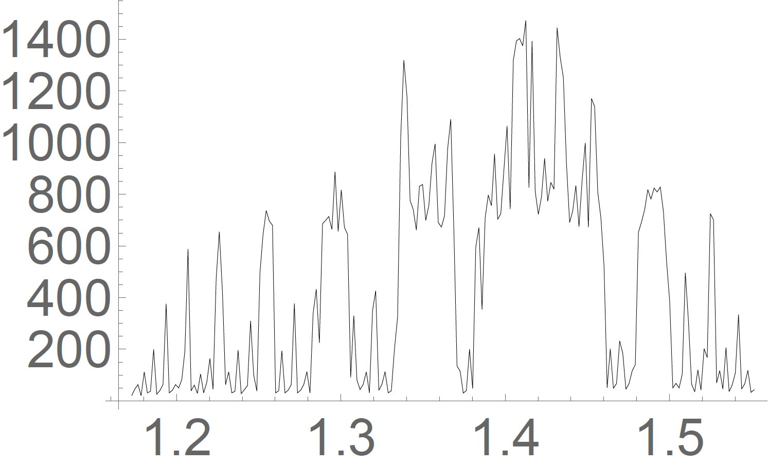
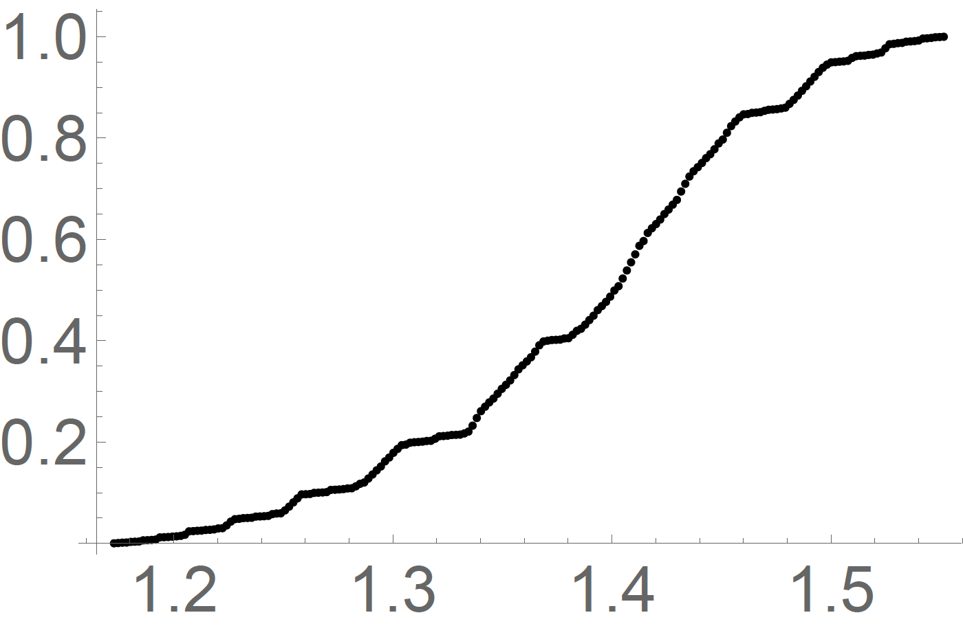
Figure 1: Graph, frequency, and distribution of $z(x)/x^{\gamma}$

As observed in the first figure of Figure 1, there are values of $x$ where the ratios are locally extremal over a relatively large interval, and we prove that their limits are as identified in (1). The local minima are obtained at $x_{1}=2^{n-1}$ for each $n\geq 2$, and the local maxima are obtained at $x_{2}=\sum_{k=0}^{t}2^{n-2k-1}$ where $t=\lfloor(n-1)/2\rfloor$. The sample interval $262144\leq x<349525$ used in the second figure of Figure 1 is obtained at these values where $n=19$.

The topic has a purely combinatorial interpretation as well. Consider the sets $\widetilde{\mathcal{E}}$ defined in Lemma 1.2, and notice that $\widetilde{\mathcal{E}}$ is lexicographically ordered; see Definition 2.4. We may ask ourselves how many tuples in $\widetilde{\mathcal{E}}$ that are “less than” a certain tuple in $\widetilde{\mathcal{E}}$ and have no consecutive $1$s, and the fluctuating behavior of the distribution of such tuples in $\widetilde{\mathcal{E}}$ is precisely as presented in Figure 1.

In [1], the notion of regular sequences is introduced, and proved in [12] is an asymptotic formula of $\sum_{k=1}^{x}\chi(k)$ in full generality where $\chi(k)$ is a regular sequence. It turns out that the fluctuation behavior is a common feature of the summatory function of a regular sequence, and there are many examples of summatory functions in the literature that have similar fluctuation behaviors; see [6, 8, 19, 16]. This setup in [12] applies to some cases of ours. For the case of Zeckendorf binary expansions, the counting function $z(x)$ is equal to $\sum_{k=0}^{x-1}\chi(k)$ where $\chi$ is the regular sequence defined by $\chi(k)=1$ if the binary expansion of $k$ is Zeckendorf, and $\chi(k)=0$ otherwise. The asymptotic formula involves a fluctuation factor as a continuous periodic function on the real numbers, and we follow their formulation of the asymptotic formula, which has been standard in the literature; see Section 6.

The authors of [12] describe the fluctuation factor as a Fourier expansion. In the context of the Mellin-Perron summation formula, the description of the Fourier coefficients is given in terms of the coefficients of Laurent expansions of the Dirichlet series $\frac{1}{s}\left(\chi(0)+\sum_{k=1}^{\infty}\chi(k)/k^{s}\right)$ at special points that line up in a vertical line in the complex plane. One of our main goals is to obtain exact bounds on the fluctuation factor. However, it does not seem feasible for us to use the Fourier expansion formulation and obtain exact bounds. Moreover, the current notion of regular sequences in the literature is formulated for base-$N$ expansions, and hence, the asymptotic formula in [12] does not apply to the expansions in terms of the fundamental sequences of periodic Zeckendorf collections. We shall introduce an example in Section 5 where we count certain expressions under non-base-$N$ expansions.

Introduced in Theorem 3.9 is a formula for the counting function $z(x)$ in full generality, and we call it the duality formula. We use the duality formula to obtain exact bounds on the fluctuation factor of $z(x)$ rather than the Fourier expansions described in [12]. The duality formula is a manifestation of the phenomenon that the coefficient functions of $\mathcal{E}$ themselves bring out their own fundamental sequence $\{H_{k}\}_{k=1}^{\infty}$ into the formula of $z(x)$. For example, as stated in Lemma 1.2, the Fibonacci sequence is the fundamental sequence of the coefficient functions that do not have consecutive $1$s, and the number of Zeckendorf binary expansions $<x$ is written as a sum of Fibonacci terms in a fashion similar to the binary expansion of $x$; see Lemma 1.5 below. A subset of $\mathbb{N}$ is called an index subset in the context of series expansions, and an element of the subset is called an index.

Lemma 1.5 (Duality formula).

Let $A$ be a finite subset of indices. If $A$ contains no adjacent indices, define $\bar{A}:=A$. If there is a largest index $j\in A$ such that $j+1\in A$, then define $\bar{A}:=\{k\in A:k\geq j\}$. Then, $z(\sum_{k\in A}2^{k-1})=\sum_{k\in\bar{A}}F_{k}$.

For example, $100=2^{2}+2^{5}+2^{6}=\widetilde{H}_{3}+\widetilde{H}_{6}+\widetilde{H}_{7}$, and the indices of non-zero coefficients are $A=\{3,6,7\}$. Thus, $\bar{A}=\{6,7\}$, and $z(100)=F_{6}+F_{7}=F_{8}=34$.

Let us formulate the counting function $z(x)$ using a continuous real-valued function as done in [12]. Recall the example of the Zeckendorf binary expansions and the formulas (1). By [12, Theorem A], there is a continuous real-valued function $\Phi:\mathbb{R}\to\mathbb{R}$ such that $z(x)\sim x^{\gamma}\Phi(\{\log_{2}(x)\})$ where $\{\log_{2}(x)\}$ denotes the fractional part of $\log_{2}(x)$, and the authors of [12] describe $\Phi(t)$ as a Fourier series. As explained earlier, we use the duality formula, rather than the Fourier series description, and we also use the generalized Zeckendorf expansions for the real numbers in the interval $(0,1)$, which is developed in [4]; see Section 2.3. In this section we state our results on the properties of $\Phi$ in Theorem 1.6 below, and its technical versions are found in Theorem 4.5, 4.12, and 4.13.

Theorem 1.6.

Let $z(x)$ be the counting function defined in Theorem 1.4. Then, $z(x)\sim x^{\gamma}\Phi(\{\log_{\widetilde{\phi}}(x)\})$ for some positive real numbers $\gamma<1$ and $\widetilde{\phi}>1$ and a continuous function $\Phi$. Moreover, $\Phi$ is differentiable almost everywhere with respect to Lebesgue measure, and there are explicit criteria in terms of the generalized Zeckendorf expansion of a real number $y$ for determining whether $\Phi$ is differentiable at $y$ or not, and whether $\Phi$ has a local maximum, a local minimum, or neither at $y$.

When the quotient $z(x)/x^{\gamma}$ is calculated, we noticed that its values are naturally transitioned to the quotient of two real numbers in the interval $(0,1)$, e.g., for the Zeckendorf binary expansions,

$$\frac{F_{9}+F_{6}+F_{2}}{\left(2^{8}+2^{5}+2\right)^{\gamma}}=\frac{\alpha\omega+\alpha\omega^{2}+\alpha\omega^{6}+E}{\left(\frac{1}{2}+\frac{1}{2^{2}}+\frac{1}{2^{6}}\right)^{\gamma}}=\alpha\,\frac{\omega+\omega^{2}+\omega^{6}+E/\alpha}{\left(\frac{1}{2}+\frac{1}{2^{2}}+\frac{1}{2^{6}}\right)^{\gamma}}$$ (2)

where $\omega=1/\phi$, $\alpha=(3\phi+1)/5$, and $E$ is a relatively smaller quantity. Notice that properly estimating the value of the last expression in (2) for general cases may rely on the uniqueness of the expansions of the real numbers in the numerator and the denominator, and it leads us naturally to the generalized Zeckendorf expansions of real numbers. Motivated from the non-constant quotient factor of the last expression in (2), we define a function on the interval $(0,1)$ to represent the factor, and denote it by $\delta^{*}:(0,1)\to\mathbb{R}$; see Definition 3.17. Theorem 4.5, 4.12, and 4.13 are stated for $\delta^{*}$. For the case of the Zeckendorf binary expansions, the relationship between the continuous functions can be $\Phi(\{\log_{2}(x)\})\sim\alpha\delta^{*}(2^{\{\log_{2}{x}\}-1})$ where $\Phi$ is the function appearing in [12].

As demonstrated in the case of Zeckendorf binary expansions, the factor $\delta^{*}$ is infinitesimally fluctuating for the general cases as well, and the main tools for analyzing the fluctuations were the generalized Zeckendorf expansions for the real numbers (see the work toward Definition 3.17) and Lemma 4.16, which describes a sufficient condition for $\delta^{*}$ having a higher value.

The remainder of the paper is organized as follows. In Section 2, we review the generalized Zeckendorf expansions for the positive integers and the real numbers in $(0,1)$. These contents are also available in [4], but for the readability of our work we review the contents in this paper. In Section 3, the setup of two generalized Zeckendorf expressions is introduced for the positive integers and for the interval $(0,1)$, and in this setup the duality formula and the transition from the integers to the real numbers are introduced. In Section 4, the main results Theorem 1.4 and 1.6 are proved. In Section 5, calculations for the Zeckendorf binary expansions and two more pairs of collections are demonstrated, one of which is a pair with non-base-$N$ expansions. In Section 6, we conclude the paper discussing the generalization of regular sequences and their summatory functions.

2 Generalized Zeckendorf expansions

We shall review the definitions and results related to the generalized Zeckendorf expansions for positive integers that are periodic, which are also available in [4], and by [4, Theorem 7], our definition is equivalent to the definition introduced in [17, Definition 1.1]. We also review the definitions and results related to the generalized Zeckendorf expansions for the real numbers in the interval $\mathbf{I}:=(0,1)$ that are periodic; see [4] for non-periodic ones for $\mathbf{I}$.

2.1 Notation and definitions

We identify a sequence of numbers with an infinite tuple, and denote its terms using subscripts. For example, the sequence of positive odd integers is denoted by $Q=(1,3,5,7,\dots)$, and we use subscripts to denote its values, e.g., $Q_{3}=5$. We may define a sequence by describing $Q_{k}$ where $k$ is assumed to be an index $\geq 1$, e.g., the earlier example is the sequence given by $Q_{k}=2k-1$. Recall coefficient functions from Definition 1.1. Given a coefficient function $\epsilon$ and a sequence $Q$, we denote $\sum\epsilon Q$ to be the formal sum $\sum_{k=1}^{\infty}\epsilon_{k}Q_{k}$.

Given two coefficient functions $\epsilon$ and $\mu$, we define $\epsilon+\mu$ to be the coefficient function such that $(\epsilon+\mu)_{k}=\epsilon_{k}+\mu_{k}$ for $k\geq 1$, and $\epsilon-\mu$ to be the coefficient function such that $(\epsilon-\mu)_{k}=\epsilon_{k}-\mu_{k}$ for $k\geq 1$ if $\epsilon_{k}\geq\mu_{k}$ for all $k\geq 1$. Given $c\in\mathbb{N}_{0}$, we define $c\epsilon:=(c\epsilon_{1},c\epsilon_{2},\dots)$.

Definition 2.1.

Let $\beta^{i}$ be the coefficient function such that $\beta^{i}_{k}=0$ for all $k\neq i$ and $\beta_{i}^{i}=1$, and call it the $i$th basis coefficient function; in particular, $\beta^{i}_{k}$ does not denote the $i$th power of an integer.

Definition 2.2.

For coefficient functions $\epsilon$, we use the bar notation $\bar{a}$ to represent the repeating entries. For example, $\epsilon=(1,2,3,\bar{0})$ is the coefficient function such that $\epsilon_{k}=0$ for all $k>3$, and we denote it by $\epsilon=(1,2,3)$ as well. If $\epsilon=(\bar{0},1,2,3)$, then it means that there is an index $n$ such that $\epsilon_{k}=0$ for $1\leq k\leq n$, and $\epsilon_{n+j}=j$ for $1\leq j\leq 3$. We use the simpler notation $0$ for the zero coefficient function $(\bar{0})$. If there is an index $M$ such that $\epsilon_{k}=0$ for all $k>M$, $\epsilon$ is said to have finite support.

Definition 2.3.

Let $\epsilon$ be a coefficient function, and let $m\leq n$ be two positive integers. Define $\mathrm{rev}_{n}(\epsilon)$ to be the coefficient function $(\epsilon_{n},\epsilon_{n-1},\dots,\epsilon_{1})$.

Define $\operatorname{res}_{m}(\epsilon)$ and $\operatorname{res}^{m}(\epsilon)$ to be the coefficient functions such that $\operatorname{res}_{m}(\epsilon)_{k}=0$ for all $k>m$, $\operatorname{res}_{m}(\epsilon)_{k}=\epsilon_{k}$ for all $1\leq k\leq m$, $\operatorname{res}^{m}(\epsilon)_{k}=\epsilon_{k}$ for all $k\geq m$, and $\operatorname{res}^{m}(\epsilon)_{k}=0$ for all $1\leq k<m$. Also we define $\operatorname{res}^{0}(\epsilon):=\epsilon$, $\operatorname{res}_{0}(\epsilon)=0$, and $\operatorname{res}_{n}^{m}(\epsilon)$ to be the coefficient function such that $\operatorname{res}_{n}^{m}(\epsilon)_{k}=\epsilon_{k}$ for all $m\leq k\leq n$ and $\operatorname{res}_{n}^{m}(\epsilon)_{k}=0$ for other indices $k$.

2.2 Generalized Zeckendorf expansions for positive integers

We shall use the ascending lexicographical order to define generalized Zeckendorf expansions for positive integers, and it is defined as follows.

Definition 2.4.

Given two coefficient functions $\mu$ and $\mu^{\prime}$ with finite support, if there is a largest positive integer $k$ such that $\mu_{j}=\mu^{\prime}_{j}$ for all $j>k$ and $\mu_{k}<\mu^{\prime}_{k}$, then we denote the property by $\mu<_{\text{a}}\mu^{\prime}$.

For example, if $\mu=(1,2,10,3,7)$ and $\mu^{\prime}=(1,3,1,4,7)$, then $\mu<_{\text{a}}\mu^{\prime}$ since $\mu_{4}<\mu^{\prime}_{4}$ and $\mu_{5}=\mu^{\prime}_{5}$.

Definition 2.5.

We define an ascendingly-ordered collection $\mathcal{E}$ of coefficient functions to be a set of coefficient functions with finite support ordered by the ascending lexicographical order that contains the zero coefficient function and all basis coefficient functions $\beta^{i}$.

Let $\mathcal{E}$ be an ascendingly-ordered collection, and let $\mu\in\mathcal{E}$. The smallest coefficient function in $\mathcal{E}$ that is greater than $\mu$, if (uniquely) exists, is called the immediate successor of $\mu$ in $\mathcal{E}$, and we denote it by $\widetilde{\mu}$. The largest coefficient function in $\mathcal{E}$ that is less than $\mu$, if (uniquely) exists, is called the immediate predecessor of $\mu$ in $\mathcal{E}$, and we denote it by $\widehat{\mu}$. In particular, $\hat{\beta}^{n}$ shall denote the immediate predecessor of the $n$th basis coefficient function $\beta^{n}$ for each $n\geq 2$, if (uniquely) exists.

Definition 2.6.

Let $\mu$ be an element of an ascendingly-ordered collection. If $\mu\neq 0$, the largest index $n$ such that $\mu_{n}\neq 0$ is called the order of $\mu$, denoted by $\mathrm{ord}(\mu)$. If $\mu=0$, we define $\mathrm{ord}(\mu)=0$.

By definition, an ascendingly-ordered collection $\mathcal{E}$ contains all the basis coefficient functions, i.e., $\beta^{n-1}\in\mathcal{E}$ for $n\geq 2$, and hence, the immediate predecessor $\hat{\beta}^{n}$, if exists, has a non-zero value at index $n-1$, i.e., $\mathrm{ord}(\hat{\beta}^{n})=n-1$.

Definition 2.7.

Let $\mathcal{E}$ be an ascendingly-ordered collection of coefficient functions. The collection is called Zeckendorf if it satisfies the following:

1. For each $\mu\in\mathcal{E}$ there are at most finitely many coefficient functions that are less than $\mu$.

2. Given $\mu\in\mathcal{E}$, if its immediate successor $\widetilde{\mu}$ is not $\beta^{1}+\mu$, then there is an index $n\geq 2$ such that $\operatorname{res}_{n-1}(\mu)=\hat{\beta}^{n}$ and $\widetilde{\mu}=\beta^{n}+\operatorname{res}^{n}(\mu)$.

We also call $\mathcal{E}$ a Zeckendorf collection for positive integers.

Surprisingly enough, it turns out that a Zeckendorf collection for positive integers is completely determined by the subset $\{\hat{\beta}^{n}:n\geq 2\}$, which is the meaning of Theorem 2.8 below.

Theorem 2.8 ([4], Definition 8 & Corollary 9).

Given coefficient functions $\theta^{n}$ of order $n-1$ for $n\geq 2$, there is a unique Zeckendorf collection for positive integers such that $\hat{\beta}^{n}=\theta^{n}$ for each $n\geq 2$.

Let us demonstrate the Zeckendorf collection for positive integers determined by $\theta^{n}$, which have a common periodic structure.

Definition 2.9.

Let $L=(e_{1},\dots,e_{N})$ be a list of non-negative integers where $N\geq 2$ and $e_{1}\neq 0$, and let $\beta^{*}$ be the coefficient function such that $\beta^{*}_{k}=e_{j}$ where $1\leq j\leq N$ and $k\equiv j\ (\mathrm{mod}\ N)$. Given $n\geq 2$, define $\theta^{n}:=\mathrm{rev}_{n-1}(\beta^{*})$.

For an integer $n\geq 2$, a coefficient function $\zeta$ is called a proper $L$-block at index $n-1$ if there is an index $k\leq n-1$ such that $\operatorname{res}^{k+1}(\zeta)=\operatorname{res}^{k+1}(\theta^{n})$, $\zeta_{k}<\theta^{n}_{k}$, and $\operatorname{res}_{k-1}(\zeta)=0$. The index interval $[k,n-1]$ is called the support interval of the proper $L$-block $\zeta$ at index $n-1$. The coefficient functions $\theta^{n}$ for $n\geq 2$ are called maximal $L$-blocks, and the index interval $[1,n-1]$ is called the support interval of the maximal $L$-block at index $n-1$. Both proper and maximal $L$-blocks are called $L$-blocks, and two $L$-blocks $\zeta$ and $\xi$ are said to be disjoint if their support intervals are disjoint sets of indices.

Theorem 2.10 ([4], Theorem 7).

Let $L$ and $\theta^{n}$ for integers $n\geq 2$ be as defined in Definition 2.9. Then, the collection $\mathcal{E}$ consisting of the sums of finitely many disjoint $L$-blocks is a Zeckendorf collection for positive integers such that $\hat{\beta}^{n}=\theta^{n}$ for $n\geq 2$.

Definition 2.11.

Let $L$ and $\mathcal{E}$ be as defined in Theorem 2.10. The collection $\mathcal{E}$ is called the periodic Zeckendorf collection for positive integers determined by $L$.

Definition 2.12.

Let $L$ be the list defined in Definition 2.9. Let $\epsilon=\sum_{m=1}^{n}\zeta^{m}$ where $\zeta^{m}$ are disjoint $L$-blocks at index $i_{m}$ such that $i_{m}<i_{m+1}$ for $1\leq m<n$. This expression is called an $L$-block decomposition, and if $\epsilon\neq 0$, the support intervals of $\zeta^{m}$ form a partition of $[1,i_{n}]$, and $\zeta^{n}\neq 0$, the summation is called the (full) $L$-block decomposition of $\epsilon$. If $\epsilon\neq 0$ and $\zeta^{m}$ are non-zero disjoint $L$-blocks, then the summation is called the non-zero $L$-block decompositionof $\epsilon$. The expression $\mu+\tau$ is called an $L$-decomposition if $\sum_{m=1}^{n}\zeta^{m}$ is an $L$-block decomposition, $\mu=\sum_{m=1}^{s}\zeta^{m}$, and $\tau=\sum_{m=t}^{n}\zeta^{m}$ where $1\leq s<t\leq n$.

Example 2.13.

Let $L=(2,3,0)$, and let $\mathcal{E}$ be the periodic Zeckendorf collection for positive integers determined by $L$. Then, $\beta^{*}=(2,3,0,2,3,0,2,3,0,\dots)$, and the following are examples of the immediate predecessors:

$$\hat{\beta}^{2}=(2),\ \hat{\beta}^{3}=(3,2),\ \hat{\beta}^{4}=(0,3,2),\ \hat{\beta}^{5}=(2,0,3,2),\ \hat{\beta}^{9}=(3,2,0,3,2,0,3,2).$$

Listed below are examples of proper $L$-blocks at index $5$:

$$\zeta^{1}=(0,0,0,0,2),\ \zeta^{2}=(0,0,0,2,2),\ \zeta^{3}=(0,0,0,3,2).$$

The support intervals of $\zeta^{k}$ for $k=1,2,3$ are $[4,5]$, $[4,5]$, and $[2,5]$, respectively. Stated below are two examples of the sum of finitely many disjoint $L$-blocks where a semicolon is inserted instead of a comma to indicate the end of the support interval of a block, and their immediate successors are stated below as well:

$$\epsilon=(2,0,3,2;0;0,0,3,2;2,2;1),\ \tau=(1,0,3,2;0;0,0,3,2;2,2;1)$$

$$\widetilde{\epsilon}=(0;0;0;0;1;0,0,3,2;2,2;1),\ \widetilde{\tau}=(2,0,3,2;0;0,0,3,2;2,2;1).$$

Given a collection $\mathcal{E}$ of coefficient functions with finite support and a sequence $G$ of positive integers, let $\mathrm{eval}_{G}:\mathcal{E}\to\mathbb{N}_{0}$ be the evaluation map given by $\epsilon\mapsto\sum\epsilon G$. The weak converse of Zeckendorf’s theorem for Zeckendorf collections for positive integers is stated below. Recall Definition 2.4.

Theorem 2.14 ([4], Theorem 16, Lemma 3 & 37).

Let $\mathcal{E}$ be a Zeckendorf collection for positive integers with the immediate predecessors $\hat{\beta}^{n}$ for  $n\geq 2$. Then, there is a unique increasing sequence $H$ of positive integers such that $\mathrm{eval}_{H}:\mathcal{E}\to\mathbb{N}_{0}$ is bijective. Moreover, for each $n\geq 2$,

$$H_{n}=H_{1}+\sum\hat{\beta}^{n}H,$$ (3)

and the map $\mathrm{eval}_{H}$ is increasing, i.e., $\epsilon<_{\text{a}}\delta$ if and only if $\mathrm{eval}_{H}(\epsilon)<\mathrm{eval}_{H}(\delta)$.

Recall Definition 1.1. Then, by Theorem 2.14, given a Zeckendorf collection $\mathcal{E}$ for positive integers there is one and only one fundamental sequence of $\mathcal{E}$.

Definition 2.15.

Given a Zeckendorf collection $\mathcal{E}$ for positive integers, the expansion $n=\sum\epsilon H$ is called the $\mathcal{E}$-expansion of $n$ where $H$ is the fundamental sequence of $\mathcal{E}$.

For the collection in Example 2.13, the fundamental sequence $H$ is given by the linear recurrence $H_{n+3}=2H_{n+2}+3H_{n+1}+H_{n}$ with $(H_{1},H_{2},H_{3})=(1,3,10)$. In general, the fundamental sequence of a periodic Zeckendorf collection determined by $L=(e_{1},\dots,e_{N})$ is given by

$$H_{n}=\sum_{k=1}^{N-1}e_{k}H_{n-k}+(1+e_{N})H_{n-N},\quad n>N$$ (4)

with initial values $(H_{1},H_{2},\dots,H_{N})$ determined by (3).

Definition 2.16.

Let $L=(e_{1},\dots,e_{N})$ be the list defined in Definition 2.9. The following is called the characteristic polynomial of $L$ for positive integers:

$$x^{N}-\sum_{k=1}^{N-1}e_{k}x^{N-k}-(1+e_{N}).$$ (5)

By Descartes’ Rule of Signs, the polynomial defined in (5) has one positive simple real root $\phi$, and it is $>1$. By [4, Section 5.3.2], it is the only root with the largest modulus in the complex plane. Thus, by Binet’s formula, $H_{n}=\alpha\phi^{n}+O(\phi^{nr})$ where $\alpha$ and $r<1$ are positive real constants. Notice that the periodic Zeckendorf collection for positive integers determined by $L=(e_{1},\dots,e_{N},e_{1},\dots,e_{N})$ is equal to the collection determined by $(e_{1},\dots,e_{N})$ since they have the same immediate predecessor of $\beta^{n}$ for each $n\geq 2$.

2.3 Generalized Zeckendorf expansions for real numbers

Let us review the definitions and results for the periodic Zeckendorf collections for the real numbers in the interval $\mathbf{I}:=(0,1)$. The general definition is given in [4, Definition 10], and in this paper, we review the definition for the periodic Zeckendorf collections.

Definition 2.17.

Given two coefficient functions $\epsilon$ and $\epsilon^{\prime}$, we define the descending lexicographical order as follows. If there is a smallest positive integer $k$ such that $\epsilon_{j}=\epsilon^{\prime}_{j}$ for all $j<k$ and $\epsilon_{k}<\epsilon^{\prime}_{k}$, then we denote the property by $\epsilon<_{\text{d}}\epsilon^{\prime}$.

For example, if $\epsilon=(1,2,10,5,\dots)$ and $\epsilon^{\prime}=(1,3,1,10,\dots)$, then $\epsilon<_{\text{d}}\epsilon^{\prime}$ since $\epsilon_{2}<\epsilon^{\prime}_{2}$ and $\epsilon_{1}=\epsilon^{\prime}_{1}$.

Definition 2.18.

If $\epsilon\neq 0$ is a coefficient function, the smallest index $n$ such that $\epsilon_{n}\neq 0$ is denoted by $\mathrm{ord}^{*}(\epsilon)$. If $\epsilon=0$, we define $\mathrm{ord}^{*}(\epsilon)=\infty$.

Definition 2.19.

Let $L=(e_{1},\dots,e_{N})$ be a list of non-negative integers where $N\geq 2$ and $e_{1}\neq 0$. Given $n\geq 1$, let $\bar{\beta}^{n}$ be the coefficient function such that $\operatorname{res}_{n-1}(\bar{\beta}^{n})=0$ and $\bar{\beta}^{n}_{k}=e_{j}$ for $k\geq n$ where $1\leq j\leq N$ and $k-n+1\equiv j\ (\mathrm{mod}\ N)$, and we call $\bar{\beta}^{n}$ the maximal $L^{*}$-block at index $n$.

For an integer $n\geq 2$, a coefficient function $\zeta$ is called a proper $L^{*}$-block at index $n$ if there is an index $k\geq n$ such that $\operatorname{res}_{k-1}(\zeta)=\operatorname{res}_{k-1}(\bar{\beta}^{n})$, $\zeta_{k}<\bar{\beta}^{n}_{k}$, and $\operatorname{res}^{k+1}(\zeta)=0$. The index interval $[n,k]$ is called the support interval of the proper $L^{*}$-block $\zeta$ at index $n$. Two proper $L^{*}$-blocks $\zeta$ and $\xi$ are said to be disjoint if their support intervals are disjoint sets of indices.

The descendingly ordered collection of non-zero coefficient functions consisting of the finite or infinite sums of disjoint proper $L^{*}$-blocks is called the periodic Zeckendorf collection for $\mathbf{I}$ determined by $L$. If $\mathcal{E}$ denotes the periodic Zeckendorf collection for positive integers determined by $L$, the collection for $\mathbf{I}$ is denoted by $\mathcal{E}^{*}$.

Let $\epsilon=\sum_{m=1}^{\infty}\zeta^{m}$ where $\zeta^{m}$ are disjoint proper $L^{*}$-blocks at index $i_{m}$ such that $i_{m}<i_{m+1}$. This expression is called an $L^{*}$-block decomposition of $\epsilon$, and if the support intervals of $\zeta^{m}$ form a partition of $[1,\infty)$, the summation is called the (full) $L^{*}$-block decomposition of $\epsilon$. If $\zeta^{m}$ are non-zero disjoint proper $L^{*}$-blocks, then the summation is called the non-zero $L^{*}$-block decomposition of $\epsilon$. The expression $\mu+\tau$ is called an $L^{*}$-decomposition if $\sum_{m=1}^{\infty}\zeta^{m}$ is an $L^{*}$-block decomposition, $\mu=\sum_{m=1}^{s}\zeta^{m}$, and $\tau=\sum_{m=t}^{\infty}\zeta^{m}$ where $1\leq s<t$.

Thus, given a list $L=(e_{1},\dots,e_{N})$, we have the periodic Zeckendorf collection $\mathcal{E}$ for positive integers and the periodic Zeckendorf collection $\mathcal{E}^{*}$ for $\mathbf{I}$. The collection $\mathcal{E}$ is ascendingly ordered, and $\mathcal{E}^{*}$ is descendingly ordered. Also notice that the zero coefficient function and the maximal blocks $\bar{\beta}^{n}$ for $n\geq 1$ are not members of $\mathcal{E}^{*}$, but the zero coefficient function can be a proper $L^{*}$-block at any index $n$.

Example 2.20.

Let $L=(2,3,0)$, and let $\mathcal{E}^{*}$ be the periodic Zeckendorf collection for $\mathbf{I}$ determined by $L$. The following are examples of maximal $L^{*}$-blocks:

$$\bar{\beta}^{1}=(2,3,0,2,3,0,\dots),\ \bar{\beta}^{2}=(0,2,3,0,2,3,0,\dots),\ \bar{\beta}^{3}=(0,0,2,3,0,2,3,0,\dots).$$

Listed below are examples of proper $L^{*}$-blocks at index $4$, and semicolons are inserted to indicate the ends of the support intervals. See Definition 2.2 for the bar notation:

$$\zeta^{1}=(0;0;0;2,0;\bar{0}),\ \zeta^{2}=(0;0;0;2,2;\bar{0}),\ \zeta^{3}=(0;0;0;2,3,0,0;\bar{0}).$$

The support intervals of $\zeta^{k}$ for $k=1,2,3$ are $[4,5]$, $[4,5]$, and $[4,7]$, respectively. Stated below are two examples of coefficient functions where $\epsilon\not\in\mathcal{E}^{*}$ and $\tau\in\mathcal{E}^{*}$:

$$\epsilon=(1,2,2,\bar{0})+\bar{\beta}^{4}=(1,2,2,\overline{2,3,0}),\quad\quad\tau=(1,2,2,\overline{2,3,0,0}).$$

Lemma 2.21 ([4], Definition 10, Theorem 13).

Let $\epsilon$ be a coefficient function. Then, $\mathrm{rev}_{n}(\epsilon)\in\mathcal{E}$ for all $n\geq 1$ if and only if $\epsilon\in\mathcal{E}^{*}$ or $\epsilon=\sum_{m=1}^{n}\zeta^{m}+\bar{\beta}^{b+1}$ where $\sum_{m=1}^{n}\zeta^{m}$ is an $L^{*}$-block decomposition and $[i,b]$ is the support interval of $\zeta^{n}$.

Recall Definition 2.17.

Theorem 2.22 ([4], Theorem 24).

Let $\mathcal{E}^{*}$ be the periodic Zeckendorf collection for $\mathbf{I}$ determined by $L=(e_{1},\dots,e_{N})$. Then, there is a unique decreasing sequence $Q$ of real numbers in $\mathbf{I}$ such that the map $\mathrm{eval}_{Q}:\mathcal{E}^{*}\to\mathbf{I}$ given by $\epsilon\mapsto\sum\epsilon Q$ is bijective, and the map $\mathrm{eval}_{Q}$ is increasing, i.e., $\epsilon<_{\text{d}}\delta$ if and only if $\mathrm{eval}_{Q}(\epsilon)<\mathrm{eval}_{Q}(\delta)$.

Moreover, for each $n\geq 1$,

$$Q_{n}=\sum\bar{\beta}^{n+1}Q,\ \text{and}\ Q_{n}=\omega^{n}$$ (6)

where $\omega$ is the (only) positive real zero of the polynomial

$$-1+\sum_{k=1}^{N-1}e_{k}x^{k}+(1+e_{N})x^{N}.$$ (7)

Definition 2.23.

Let $\mathcal{E}^{*}$ be a periodic Zeckendorf collection for $\mathbf{I}$. The sequence $Q$ defined in Theorem 2.22 is called the fundamental sequence of $\mathcal{E}^{*}$, and the polynomial (7) is called the characteristic polynomial of $L$ for $\mathbf{I}$.

For the collection in Example 2.20, the fundamental sequence $Q$ is given by the linear recurrence $Q_{n}=2Q_{n+1}+3Q_{n+2}+Q_{n+3}$, and their initial values are given by the formula in (6). In general, the fundamental sequence of the periodic Zeckendorf collection for $\mathbf{I}$ determined by $L=(e_{1},\dots,e_{N})$ is given by

$$Q_{n}=\sum_{k=1}^{N-1}e_{k}Q_{n+k}+(1+e_{N})Q_{n+N},\quad n\geq 1.$$ (8)

The polynomial in (7) is a reciprocal version of the polynomial $f(x)$ in (5), i.e., it is equal to $-x^{N}f(1/x)$. Thus, it has a positive simple real zero $\omega<1$, and it is the only zero with the smallest modulus.

For the remainder of Section 2.3, let $\mathcal{E}^{*}$ be the periodic Zeckendorf collection for $\mathbf{I}$ determined by $L$, and let $Q$ denote the fundamental sequence of $\mathcal{E}^{*}$. The results introduced below will be used in Section 4, but they are introduced here in order to provide the reader with an opportunity to become more familiar with generalized Zeckendorf expansions of real numbers.

Definition 2.24.

If $\epsilon\in\mathcal{E}^{*}$, we define $\mathrm{inf}_{\mathcal{E}^{*}}(\epsilon)$ as follows. If $\epsilon$ does not have finite support, then $\mathrm{inf}_{\mathcal{E}^{*}}(\epsilon):=\epsilon$. If $c$ is the largest index such that $\epsilon_{c}\geq 1$, then $\mathrm{inf}_{\mathcal{E}^{*}}(\epsilon)=\operatorname{res}_{c}(\epsilon)-\beta^{c}+\bar{\beta}^{c+1}$, which is not a member of $\mathcal{E}^{*}$. If there is no confusion, let $\inf$ denote $\inf_{\mathcal{E}^{*}}$.

The long recursion (6) implies the following lemma, and we leave the proof to the reader.

Lemma 2.25.

If $\epsilon\in\mathcal{E}^{*}$, then $\sum\epsilon Q=\sum\inf(\epsilon)Q$.

Recall the restriction notation from Definition 2.3 and $L^{*}$-decompositions from Definition 2.19. Throughout the proof of Lemma 2.26, we use the increasing property of $\mathrm{eval}_{Q}$ defined in Theorem 2.22.

Lemma 2.26.

Let $\epsilon\in\mathcal{E}^{*}$, let $x=\sum\epsilon Q>0$, and let $\Delta x$ be a sufficiently small positive real number such that $x+\Delta x<1$ and $x-\Delta x>0$. If $x+\Delta x=\sum\epsilon^{+}Q$ for $\epsilon^{+}\in\mathcal{E}^{*}$, and $n$ is the largest integer $\geq 0$ such that $\operatorname{res}_{n}(\epsilon)=\operatorname{res}_{n}(\epsilon^{+})$, then $n\to\infty$ as $\Delta x\to 0$. If $x-\Delta x=\sum\epsilon^{-}Q$ for $\epsilon^{-}\in\mathcal{E}^{*}$, and $n$ is the largest integer $\geq 0$ such that $\operatorname{res}_{n}(\mathrm{inf}(\epsilon))=\operatorname{res}_{n}(\epsilon^{-})$, then $n\to\infty$ as $\Delta x\to 0$.

Proof.

Let $\epsilon=\sum_{m=1}^{\infty}\zeta^{m}$ be an $L^{*}$-block decomposition, and let $[i_{m},b_{m}]$ be the support interval of $\zeta^{m}$. Notice that given $m\geq 1$, there is a smallest index $k_{m}>b_{m}$ such that $\bar{\beta}^{i_{m}}_{k_{m}}>0$, and that $b_{m}$ and $k_{m}$ approach $\infty$ as $m\to\infty$.

Let $\Delta x=\sum\epsilon^{0}Q$ where $\mathrm{ord}^{*}(\epsilon^{0})=t$, and let $T$ be the largest index such that $k_{T}<t$ where $t$ is sufficiently large. Then, $\Delta x<Q_{k_{T}}$. Recall from Definition 2.19 the support intervals of proper $L^{*}$-blocks. Then, $\xi:=\zeta^{T}+\beta^{b_{T}}$ is a proper $L^{*}$-block, and its support interval is either $[i_{T},b_{T}]$ or $[i_{T},k_{T}]$, and hence, $\sum_{m=1}^{T-1}\zeta^{m}+\xi+\beta^{k_{T}}\in\mathcal{E}^{*}$. Thus,

$$x=\sum\left(\textstyle\sum_{m=1}^{\infty}\zeta^{m}\right)\displaystyle Q<x+\Delta x<\displaystyle\sum\left(\textstyle\sum_{m=1}^{T}\zeta^{m}\right)Q+Q_{b_{T}}+\Delta x<\displaystyle\sum\left(\textstyle\sum_{m=1}^{T-1}\zeta^{m}\right)Q+\displaystyle\sum\xi Q+Q_{k_{T}}.$$

By Theorem 2.22, $\textstyle\sum_{m=1}^{\infty}\zeta^{m}<_{\text{d}}\epsilon^{+}<_{\text{d}}\textstyle\sum_{m=1}^{T-1}\zeta^{m}+\xi+\beta^{k_{T}}$, and by the definition of the lexicographical order, we have $\operatorname{res}_{b_{T-1}}(\epsilon^{+})=\textstyle\sum_{m=1}^{T-1}\zeta^{m}=\operatorname{res}_{b_{T-1}}(\epsilon)$. Notice that as $\Delta x\to 0$, we have $t\to\infty$ and $T\to\infty$, and hence, $b_{T-1}\to\infty$.

Let us prove the statement about $x-\Delta x$. Suppose that $\epsilon=\sum_{m=1}^{\infty}\zeta^{m}$ is the non-zero $L^{*}$-block decomposition. Then, $\mathrm{inf}(\epsilon)=\epsilon$, and

$$x=\sum\left(\textstyle\sum_{m=1}^{\infty}\zeta^{m}\right)\displaystyle Q>x-\Delta x>\displaystyle\sum\left(\textstyle\sum_{m=1}^{T-1}\zeta^{m}\right)Q+\sum\zeta^{T}Q-\Delta x>\displaystyle\sum\left(\textstyle\sum_{m=1}^{T-1}\zeta^{m}\right)Q.$$

As in the earlier case, we have $\operatorname{res}_{b_{T-1}}(\epsilon^{-})=\textstyle\sum_{m=1}^{T-1}\zeta^{m}=\operatorname{res}_{b_{T-1}}(\epsilon)$, and $b_{T-1}\to\infty$ as $t\to\infty$.

Suppose that $\epsilon=\sum_{m=1}^{\ell}\zeta^{m}$ is the non-zero $L^{*}$-block decomposition, and let $c$ be the largest index such that $\zeta^{\ell}_{c}\geq 1$. Then, $\mathrm{inf}(\epsilon)=\sum_{m=1}^{\ell-1}\zeta^{m}+\xi+\bar{\beta}^{c+1}$ where $\xi=\zeta^{\ell}-\beta^{c}$. Then, there is a largest index $p$ such that $p<t$ and $c+1\equiv p\ (\mathrm{mod}\ N)$ where $N$ is the length of $L$, and hence, by the periodic structure of the entries of $\bar{\beta}^{c+1}$, we have $\bar{\beta}^{c+1}=\operatorname{res}_{p-1}(\bar{\beta}^{c+1})+\bar{\beta}^{p}$. Thus,

$$x=\sum\mathrm{inf}(\epsilon)Q>x-\Delta x=\displaystyle\sum\left(\textstyle\sum_{m=1}^{\ell-1}\zeta^{m}\right)Q+\sum\xi Q+\sum\operatorname{res}_{p-1}(\bar{\beta}^{c+1})Q+\sum\bar{\beta}^{p}Q-\Delta x$$

$$>\displaystyle\sum\left(\textstyle\sum_{m=1}^{\ell-1}\zeta^{m}\right)Q+\sum\xi Q+\sum\operatorname{res}_{p-1}(\bar{\beta}^{c+1})Q=\sum\operatorname{res}_{p-1}(\mathrm{inf}(\epsilon))Q.$$

Thus, $\sum(\textstyle\sum_{m=1}^{\ell-1}\zeta^{m}+\zeta^{\ell})Q>\sum\epsilon^{-}Q>\sum\operatorname{res}_{p-1}(\mathrm{inf}(\epsilon))Q$. It’s clear that $\operatorname{res}_{c-1}(\epsilon)=\operatorname{res}_{c-1}(\epsilon^{-})=\operatorname{res}_{c-1}(\mathrm{inf}(\epsilon))$ and $\epsilon^{-}_{c}=\zeta^{\ell}_{c}-1=\mathrm{inf}(\epsilon)_{c}$. Thus, $\epsilon^{-}=\operatorname{res}_{c}(\epsilon^{-})+\operatorname{res}^{c+1}(\epsilon^{-})$ is an $L^{*}$-decomposition, and hence, $\operatorname{res}^{c+1}(\epsilon^{-})$ is a member of $\mathcal{E}^{*}$. By Theorem 2.22, $\sum\epsilon^{-}Q>\sum\operatorname{res}_{p-1}(\mathrm{inf}(\epsilon))Q$ implies $\operatorname{res}_{p-1}(\mathrm{inf}(\epsilon))<_{\text{d}}\epsilon^{-}$, and hence, $\operatorname{res}^{c+1}_{p-1}(\bar{\beta}^{c+1})=\operatorname{res}^{c+1}_{p-1}(\mathrm{inf}(\epsilon))<_{\text{d}}\operatorname{res}^{c+1}(\epsilon^{-})$. Thus, we have $\operatorname{res}^{c+1}_{p-1}(\bar{\beta}^{c+1})<_{\text{d}}\operatorname{res}^{c+1}(\epsilon^{-})<_{\text{d}}\bar{\beta}^{c+1}$, and hence, $\operatorname{res}_{p-1}(\epsilon^{-})=\operatorname{res}_{p-1}(\mathrm{inf}(\epsilon))$. Since $p\to\infty$ as $t\to\infty$, we prove the result. ∎

Acknowledgments

The author would like to thank the referees who brought attention to the works that are related to the author’s work.

3 Generalized Zeckendorf expressions

3.1 Expressions for positive integers

Throughout this section, let $\mathcal{E}$ and $\widetilde{\mathcal{E}}$ be periodic Zeckendorf collections for positive integers determined by lists $L=(e_{1},\dots,e_{N})$ and $\widetilde{L}=(\widetilde{e}_{1},\dots,\widetilde{e}_{M})$, respectively, such that $\mathcal{E}$ is a proper subcollection of $\widetilde{\mathcal{E}}$. Let $H$ and $\widetilde{H}$ be their fundamental sequences, respectively. Let $\hat{\beta}^{n}$ and $\hat{\theta}^{n}$ be the immediate predecessor of $\beta^{n}$ in $\mathcal{E}$ and $\widetilde{\mathcal{E}}$, respectively. Recall from Definition 2.15 that $\sum\epsilon\widetilde{H}$ is called an $\widetilde{\mathcal{E}}$-expansion if $\epsilon\in\widetilde{\mathcal{E}}$, and if, in addition, $\epsilon\in\mathcal{E}$, then the summation, which is written in terms of $\widetilde{H}$, is called an $\mathcal{E}$-expression. The main object of this paper is the function that counts the number of positive integers $<x$ whose $\widetilde{\mathcal{E}}$-expansion is an $\mathcal{E}$-expression.

The proofs of Proposition 3.1, Lemma 3.8, and Theorem 3.9 given below in this section remain valid for non-periodic Zeckendorf collections. The main result of this paper is for periodic ones, and they are stated for periodic collections.

Proposition 3.1.

Let $\widetilde{\mathcal{E}}$ and $\mathcal{E}$ be Zeckendorf collections for positive integers. Then, the collection $\mathcal{E}$ is a subcollection of $\widetilde{\mathcal{E}}$ if and only if the immediate predecessors $\hat{\beta}^{n}$ in $\mathcal{E}$ are members of $\widetilde{\mathcal{E}}$ for $n\geq 2$.

Proof.

If $\mathcal{E}$ is a subcollection of $\widetilde{\mathcal{E}}$, then $\hat{\beta}^{n}\in\mathcal{E}$ for $n\geq 2$ are members of $\widetilde{\mathcal{E}}$. Suppose that $\hat{\beta}^{n}$ for $n\geq 2$ are members of $\widetilde{\mathcal{E}}$, and let us show that $\mathcal{E}\subset\widetilde{\mathcal{E}}$. First let us show that the proper $L$-blocks are members of $\widetilde{\mathcal{E}}$. Let $n\geq 2$, and let $\hat{\beta}^{n}=\sum_{m=1}^{M}\zeta^{m}$ be the $\widetilde{L}$-block decomposition (including zero blocks); see Definition 2.9. Let $\xi$ be a non-zero proper $L$-block with support interval $[a,n-1]$, i.e., $\xi_{a}<\hat{\beta}^{n}_{a}$ and $\xi_{k}=\hat{\beta}^{n}_{k}$ for all $a<k\leq n-1$, and let us show that $\xi\in\widetilde{\mathcal{E}}$.

Notice that $a$ is contained in the support interval of $\zeta^{m_{0}}$ for some $1\leq m_{0}\leq M$, and let $[b,s]$ be the support interval where $b\leq a\leq s$. Then, $\zeta^{m_{0}}$ is a nonzero $\widetilde{L}$-block since $\xi_{a}<\hat{\beta}^{n}_{a}=\zeta^{m_{0}}_{a}$ implies that $\zeta^{m_{0}}_{a}>0$. Let $\eta$ be the coefficient function such that $\eta_{a}=\xi_{a}$, $\eta_{k}=\zeta^{m_{0}}_{k}$ for all $a<k\leq s=\mathrm{ord}(\zeta^{m_{0}})$, and $\eta_{k}=0$ for other indices $k$. Then, $\eta$ is a proper $\widetilde{L}$-block with support interval $[a,s]$ since $\eta_{a}=\xi_{a}<\hat{\beta}^{n}_{a}=\zeta^{m_{0}}_{a}\leq\hat{\theta}^{s+1}_{a}$ and $\eta_{k}=\zeta^{m_{0}}_{k}=\hat{\theta}^{s+1}_{k}$ for $a<k\leq s$. Notice that $\xi=\eta+\sum_{m=m_{0}+1}^{M}\zeta^{m}$, which is the sum of disjoint $\widetilde{L}$-blocks, i.e., $\xi\in\widetilde{\mathcal{E}}$. Moreover, the support interval of the proper $L$-block $\xi$ is $[a,n-1]$, and the (disjoint) union of the support intervals of the $\widetilde{L}$-blocks $\eta$ and $\zeta^{m}$ for $m_{0}+1\leq m\leq M$ is $[a,n-1]$ as well. Thus, in general, a disjoint sum of proper $L$-blocks is a member of $\widetilde{\mathcal{E}}$.

Let us consider the case where the sum involves a maximal $L$-block $\hat{\beta}^{c}$. Let $\epsilon$ be the sum of disjoint proper $L$-blocks $\xi^{m}$ for $1\leq m\leq T$, i.e., $\epsilon=\sum_{m=1}^{T}\xi^{m}$, and suppose that $[c,n]$ where $c>1$ is the union of the support intervals of the proper $L$-blocks $\xi^{m}$. Then, as shown earlier, the union of the support intervals of the $\widetilde{L}$-block decompositions of $\xi^{m}$ for $1\leq m\leq T$ is $J_{1}:=[c,n]$ as well. Recall that $\hat{\beta}^{c}\in\widetilde{\mathcal{E}}$, and hence, it is the $\widetilde{L}$-block decomposition, the union of whose support intervals is $J_{2}:=[1,c-1]$. Since $J_{1}$ and $J_{2}$ are disjoint, the $L$-decomposition $\hat{\beta}^{c}+\epsilon$ is an $\widetilde{L}$-decomposition, and hence, it is a member of $\widetilde{\mathcal{E}}$ as well. This proves that all $L$-block decompositions are members of $\widetilde{\mathcal{E}}$.

∎

Example 3.2.

Let us demonstrate examples of subcollections. For each of the following, we first check if $\hat{\beta}^{n}\leq_{\text{a}}\hat{\theta}^{n}$ for $n=2,\dots,7$, and check if $\hat{\beta}^{n}$ is a member of $\widetilde{\mathcal{E}}$. We use the semicolon to indicate the end of the support interval of an $\widetilde{L}$-block.

1. Let $\widetilde{L}=(1,3)$ and $L=(1,2,1)$. Then, $\hat{\beta}^{7}=(1,2;1,1;2,1)<_{\text{a}}\hat{\theta}^{7}=(3,1,3,1,3,1)$. However, $\hat{\beta}^{7}$ does not have an $\widetilde{L}$-block decomposition since $\operatorname{res}^{3}(\hat{\beta}^{7})$ has an $\widetilde{L}$-block decomposition, but $\operatorname{res}_{2}(\hat{\beta}^{7})$ does not an $\widetilde{L}$-block decomposition. Thus, $\mathcal{E}$ determined by $L$ is not a subcollection of $\widetilde{\mathcal{E}}$.

2. Let $\widetilde{L}=(3,2)$ and $L=(2,3,1)$. Then, $\hat{\beta}^{7}=(;1,3;2;1,3;2)<_{\text{a}}\hat{\theta}^{7}=(2,3,2,3,2,3)$, and $\hat{\beta}^{7}$ has an $\widetilde{L}$-block decomposition. This example is sufficient to understand that $\hat{\beta}^{n}$ is a member of $\widetilde{\mathcal{E}}$ for all $n\geq 2$.

3. Let $\widetilde{L}=(3,2)$ and $L=(3,1,2)$. Then, $\hat{\beta}^{7}=(;2;1,3;2;1,3)<_{\text{a}}\hat{\delta}^{7}=(2,3,2,3,2,3)$, and $\hat{\beta}^{7}$ has an $\widetilde{L}$-block decomposition. This example is sufficient to understand that $\hat{\beta}^{n}$ is a member of $\widetilde{\mathcal{E}}$ for all $n\geq 2$.

Let us compare the fundamental sequences of $\mathcal{E}$ and $\widetilde{\mathcal{E}}$ below. We identify later in Theorem 5.1 the values of $\alpha$ and $\widetilde{\alpha}$ that are mentioned in Theorem 3.3.

Theorem 3.3.

There are positive real numbers $\alpha$, $\widetilde{\alpha}$, $\phi$, $\widetilde{\phi}$, and $r<1$ such that

$$H_{n}=\alpha\phi^{n-1}+O(\phi^{nr}),\quad\widetilde{H}_{n}=\widetilde{\alpha}\widetilde{\phi}^{n-1}+O(\widetilde{\phi}^{nr}),\quad\text{and}\quad\lim_{n\to\infty}\frac{H_{n}}{\widetilde{H}_{n}^{\gamma}}=\frac{\alpha}{\widetilde{\alpha}^{\gamma}}>0$$ (9)

where $\gamma=\log_{\widetilde{\phi}}\phi$ and $1<\phi<\widetilde{\phi}$.

Proof.

Recall $L=(e_{1},\dots,e_{N})$ and $\widetilde{L}=(\widetilde{e}_{1},\dots,\widetilde{e}_{M})$. Let $\mathbf{b}=(e_{N},\dots,e_{1})$ and $\mathbf{\widetilde{b}}=(\tilde{e}_{M},\dots,\tilde{e}_{1})$, and let $f$ and $\tilde{f}$ be the characteristic polynomials of $L$ and $\widetilde{L}$, respectively. As explained in the paragraphs below (5), there are positive real numbers $\alpha$, $\widetilde{\alpha}$, $\phi$, $\widetilde{\phi}$, and $r$ such that (9) holds and $\phi>1$, where $\phi$ and $\widetilde{\phi}$ are the dominant positive real zeros of $f$ and $\widetilde{f}$, respectively.

Let us prove that $\widetilde{\phi}>\phi$. Since $\mathcal{E}\neq\widetilde{\mathcal{E}}$, if we duplicate the repeating blocks of $\mathcal{E}$ and $\widetilde{\mathcal{E}}$ to the length of $NM$ as follows, Proposition 3.1 implies

$$\mathbf{b}^{\prime}=(e_{N},\dots,e_{N},\dots,e_{1},e_{N},\dots,e_{1})<_{\text{a}}\mathbf{\widetilde{b}}^{\prime}=(\tilde{e}_{M},\dots,\tilde{e}_{M},\dots,\tilde{e}_{1},\tilde{e}_{M},\dots,\tilde{e}_{1}).$$

Notice that $\mathcal{E}$ is equal to the periodic Zeckendorf collection determined by the reverse of the list $\mathbf{b}^{\prime}$, which is equal to $\hat{\beta}^{1+NM}$, and $\widetilde{\mathcal{E}}$ is equal to the periodic Zeckendorf collection determined by the reverse of the list $\mathbf{\widetilde{b}}^{\prime}$, which is equal to $\hat{\theta}^{1+NM}$. By Proposition 3.1, there is a largest index $s\leq NM$ such that $\hat{\beta}^{1+NM}_{s}<\hat{\theta}^{1+NM}_{s}$. Let $f_{*}(x):=x^{NM}-(e_{1}x^{NM-1}+\cdots+e_{N-1}x+(1+e_{N}))$ be the characteristic polynomial of $\mathrm{rev}_{NM}(\mathbf{b}^{\prime})$ for positive integers. Then, the following induction step shows that $\phi$ is a zero of $f_{*}$:

$$\phi^{kN} =e_{1}\phi^{kN-1}+\cdots+e_{N-1}\phi+(1+e_{N})$$

$$\Rightarrow\phi^{kN+N} =e_{1}\phi^{kN-1+N}+\cdots+e_{N-1}\phi^{1+N}+(1+e_{N})\phi^{N}$$

$$\Rightarrow\phi^{(k+1)N} =e_{1}\phi^{(k+1)N-1}+\cdots+e_{N-1}\phi^{1+N}+e_{N}\phi^{N}+e_{1}\phi^{N-1}+\cdots+(1+e_{N}).$$

Since $\phi$ is the only positive real root of $f_{*}$, it would be sufficient to prove that $f_{*}(\widetilde{\phi})>0$.

Notice that for any integer $t>3$, $\hat{\beta}^{1+tNM}_{s+(t-1)NM}<\hat{\theta}^{1+tNM}_{s+(t-1)NM}$. For convenience, let $\hat{\beta}:=\hat{\beta}^{1+tNM}$, $\hat{\theta}:=\hat{\theta}^{1+tNM}$, $s_{*}:=s+(t-1)NM$, and $s_{1}:=1+(t-1)NM$. Let $y:=\sum\operatorname{res}^{s_{1}}(\hat{\beta})\widetilde{H}$. Below we shall establish that $\widetilde{H}_{1+tNM}-(y+\widetilde{H}_{s_{1}})$ is greater than a term $\widetilde{H}_{t_{*}}$ where $t_{*}<1+tNM$ is sufficiently close to $1+tNM$. Then, the asymptotic version of the inequality will imply that $f_{*}(\phi)$ is positive.

Notice below that if $s=1$, i.e., $s_{*}=1+(t-1)NM=s_{1}$, then $\sum\operatorname{res}_{s_{*}-1}^{s_{1}}(\hat{\beta})\widetilde{H}$ is interpreted as $0$;

$$\widetilde{H}_{(t-2)NM}+\widetilde{H}_{s_{1}}+y =\widetilde{H}_{(t-2)NM}+\widetilde{H}_{s_{1}}+\sum\operatorname{res}_{s_{*}-1}^{s_{1}}(\hat{\beta})\widetilde{H}+\sum\operatorname{res}^{s_{*}}(\hat{\beta})\widetilde{H}$$

$$=\widetilde{H}_{(t-2)NM}+\widetilde{H}_{s_{1}}+\sum\operatorname{res}_{s_{*}-1}(\hat{\beta})\widetilde{H}-\sum\hat{\beta}^{s_{1}}\widetilde{H}+\sum\operatorname{res}^{s_{*}}(\hat{\beta})\widetilde{H}.$$

Notice that by the definition of $$s \operatorname{res}^{s_{*}}(\hat{\beta}) \widetilde{L} \operatorname{res}_{s_{*}-1}(\hat{\beta})\in\widetilde{\mathcal{E}}$$, the coefficient function  is a proper -block, which implies that . Thus,

$$\widetilde{H}_{(t-2)NM}+\widetilde{H}_{s_{1}}+y <\widetilde{H}_{(t-2)NM}+\widetilde{H}_{s_{1}}+\widetilde{H}_{s_{*}}-\sum\hat{\beta}^{s_{1}}\widetilde{H}+\sum\operatorname{res}^{s_{*}}(\hat{\beta})\widetilde{H}$$

$$\leq\widetilde{H}_{(t-2)NM}-\sum\hat{\beta}^{s_{1}}\widetilde{H}+\widetilde{H}_{s_{1}}+\sum\operatorname{res}^{s_{*}}(\hat{\theta})\widetilde{H}.$$

Notice that $0<y_{1}:=\widetilde{H}_{(t-2)NM}-\sum\hat{\beta}^{s_{1}}\widetilde{H}+\widetilde{H}_{s_{1}}<\widetilde{H}_{s_{1}}$ implies there is $\epsilon^{0}\in\widetilde{\mathcal{E}}$ such that $\mathrm{ord}(\epsilon^{0})\leq s_{1}-1$ and $y_{1}=\sum\epsilon^{0}\widetilde{H}$. Let $\epsilon^{0}=\sum_{m=1}^{\ell}\zeta^{m}$ be an $\widetilde{L}$-block decomposition such that the support interval of $\zeta^{\ell}$ is $[a,s_{1}-1]$, and let us claim that $\epsilon:=\epsilon^{0}+\operatorname{res}^{s_{*}}(\hat{\theta})\in\widetilde{\mathcal{E}}$. Let $[s_{0},(t-1)NM]$ be the support interval of the proper $\widetilde{L}$-block $\operatorname{res}^{s_{*}}(\hat{\theta})$. Notice that the support interval of the $\widetilde{L}$-block $\operatorname{res}^{s_{*}}(\hat{\theta})$ may not be $[s_{*},(t-1)NM]$ or $[s_{*}-1,(t-1)NM]$, e.g., if $\widetilde{L}=(1,3,0)$ and $s_{*}=2+(t-1)NM$, then the support interval is $[s_{1}-1,(t-1)NM]$. Since $\widetilde{e}_{1}=\hat{\theta}_{s_{1}-1}>0$ and $\operatorname{res}^{s_{*}}(\hat{\theta})_{s_{1}-1}=0$, we have $s_{1}-1\leq s_{0}$. If $s_{1}\leq s_{0}$, then $\epsilon$ is a sum of two disjoint $\widetilde{L}$-blocks. If $s_{1}-1=s_{0}$, then $\hat{\theta}_{s_{1}}=\widetilde{e}_{M}$ implies that $\zeta^{\ell}+\operatorname{res}^{s_{1}}(\hat{\theta})$ forms a single $\widetilde{L}$-block. Thus, $\epsilon^{0}+\operatorname{res}^{s_{*}}(\hat{\theta})\in\widetilde{\mathcal{E}}$, and

$$\widetilde{H}_{(t-2)NM}+\widetilde{H}_{s_{1}}+y \leq\sum\epsilon^{0}\widetilde{H}+\sum\operatorname{res}^{s_{*}}(\hat{\theta})\widetilde{H}\leq\sum\hat{\theta}\widetilde{H}<\widetilde{H}_{1+tNM}$$

$$\Rightarrow\quad\widetilde{H}_{(t-2)NM} <\widetilde{H}_{tNM+1}-(y+\widetilde{H}_{s_{1}})$$

$$\Rightarrow\quad\widetilde{\phi}^{-NM-1} \leq\widetilde{\phi}^{NM}-(e_{1}\widetilde{\phi}^{NM-1}+\cdots+(1+e_{N}))+o_{t}(1).$$

This proves that $0<\widetilde{\phi}^{-NM-1}\leq f_{*}(\widetilde{\phi})$ as $t\to\infty$. Since $f_{*}(\phi)=0$, we prove that $\widetilde{\phi}>\phi$. ∎

3.2 The duality formula

Recall Lemma 1.5, which is the specialized version of the duality formula. We introduce the general version for Zeckendorf collections for positive integers, including non-periodic ones.

Definition 3.4.

Given a non-zero coefficient function $\mu$ with finite support that is not necessarily in $\widetilde{\mathcal{E}}$, we denote by $\check{\mu}$ the largest coefficient function in $\mathcal{E}$ that is $<_{\text{a}}\mu$, and we denote the immediate successor of $\check{\mu}$ in $\mathcal{E}$ by $\bar{\mu}$.

Lemma 3.5 (Mixed decomposition).

Given $\epsilon\in\widetilde{\mathcal{E}}-\mathcal{E}$, write $\epsilon=\zeta^{0}+\mu$ as an $\widetilde{L}$-decomposition such that $\mu=\sum_{m=1}^{n}\zeta^{m}$ is an $L$-block decomposition with the maximal integer $n\geq 0$. If $n\geq 1$, then let $[a,i]$ be the support interval of $\zeta^{1}$, and if $n=0$, then let $a=\mathrm{ord}(\zeta^{0})+1$. Then, $\hat{\beta}^{a}<_{\text{a}}\zeta^{0}$ and $\bar{\epsilon}=\beta^{a}+\sum_{m=1}^{n}\zeta^{m}$.

Proof.

Notice that $\epsilon\not\in\mathcal{E}$ implies that $a\geq 2$. Suppose that $\zeta^{0}<_{\text{a}}\hat{\beta}^{a}$. There is an index $j\leq a-1$ such that $\zeta^{0}_{j}<\hat{\beta}^{a}_{j}$ and $\zeta^{0}_{k}=\hat{\beta}^{a}_{k}$ for $j+1\leq k\leq a-1$. Thus, $\operatorname{res}^{j}_{a-1}(\zeta^{0})$ is a proper $L$-block with support interval $[j,a-1]$ , and this contradicts the maximality of $n$. Notice that $\zeta^{0}=\hat{\beta}^{a}$ also contradicts the maximality of $n$. Thus, $\hat{\beta}^{a}<_{\text{a}}\zeta^{0}$, and $\hat{\beta}^{a}+\sum_{m=1}^{n}\zeta^{m}<_{\text{a}}\zeta^{0}+\sum_{m=1}^{n}\zeta^{m}$. Notice that $\check{\epsilon}=\hat{\beta}^{a}+\sum_{m=1}^{n}\zeta^{m}$, and hence, $\bar{\epsilon}=\beta^{a}+\sum_{m=1}^{n}\zeta^{m}$. ∎

Example 3.6.

Let $L=(1,0)$ and $\widetilde{L}=(1,1)$. Suppose that $\epsilon=(1,1,1,0,1,0,1)$, which is a member of $\widetilde{\mathcal{E}}-\mathcal{E}$. Notice that there is no $L$-block at index $7$ in $\epsilon$, and hence, the maximal number $n$ described in Lemma 3.5 is $0$, and $a=8$. So, $\hat{\beta}^{8}<_{\text{a}}\epsilon$, and hence, $\bar{\epsilon}=\beta^{8}$.

Definition 3.7.

Given a positive integer $x$, let $R(x)$ denote the subset of non-negative integers $\sum\epsilon\widetilde{H}<x$ where $\epsilon\in\mathcal{E}$, and let $z(x)$ denote $\#R(x)$.

Lemma 3.8.

For each $\mu\in\widetilde{\mathcal{E}}$, $R(\sum\mu\widetilde{H})=R(\sum\bar{\mu}\widetilde{H})$.

Proof.

Let $y\in R(\sum\bar{\mu}\widetilde{H})$. Then $y=\sum\epsilon\widetilde{H}$ where $\epsilon\in\mathcal{E}$ and $\sum\epsilon\widetilde{H}<\sum\bar{\mu}\widetilde{H}$. By Theorem 2.14 applied to $\widetilde{\mathcal{E}}$ and the fundamental sequence $\widetilde{H}$, we have $\epsilon<_{\text{a}}\bar{\mu}$, and hence, $\epsilon\leq_{\text{a}}\check{\mu}<_{\text{a}}\bar{\mu}$. Since $\check{\mu}<_{\text{a}}\mu$, we have $\epsilon<_{\text{a}}\mu$. Thus, $y=\sum\epsilon\widetilde{H}<\sum\mu\widetilde{H}$, and hence, $y\in R(\sum\mu\widetilde{H})$.

Let $y=\sum\epsilon\widetilde{H}\in R(\sum\mu\widetilde{H})$ for some $\epsilon\in\mathcal{E}$. Then, by Theorem 2.14, $\epsilon<_{\text{a}}\mu$, and hence, $\epsilon\leq_{\text{a}}\check{\mu}<\bar{\mu}$. Thus, $y=\sum\epsilon\widetilde{H}\leq\sum\check{\mu}\widetilde{H}<\sum\bar{\mu}\widetilde{H}$, i.e., $y\in R(\sum\bar{\mu}\widetilde{H})$.

∎

Theorem 3.9 (Duality Formula).

For each $\mu\in\widetilde{\mathcal{E}}$, we have $z\left(\sum\mu\widetilde{H}\right)=\sum\bar{\mu}H$.

Proof.

By Lemma 3.8, $z(\sum\mu\widetilde{H})=z(\sum\bar{\mu}\widetilde{H})$. If Theorem 2.14 is applied to $\mathcal{E}$ and $H$, then $\mathrm{eval}_{H}$ restricts to a bijective function from $S:=\{\epsilon\in\mathcal{E}:\epsilon<_{\text{a}}\bar{\mu}\}$ to $T:=\{n\in\mathbb{N}_{0}:n<\sum\bar{\mu}H\}$. Theorem 2.14 can be applied to $\widetilde{\mathcal{E}}$ and $\widetilde{H}$ as well. Since $\mathcal{E}$ is a subcollection of $\widetilde{\mathcal{E}}$, $\mathrm{eval}_{\widetilde{H}}$ restricts to a bijective function from $S:=\{\epsilon\in\mathcal{E}:\epsilon<_{\text{a}}\bar{\mu}\}$ to $\widetilde{T}:=R(\sum\bar{\mu}\widetilde{H})$. In other words, the three subsets $S$, $T$, and $\widetilde{T}$ are bijective to each other. Thus, $z(\sum\bar{\mu}\widetilde{H})=\#\widetilde{T}=\#S=\#T=\sum\bar{\mu}H$, which proves that $z(\sum\mu\widetilde{H})=z(\sum\bar{\mu}\widetilde{H})=\sum\bar{\mu}H$.

∎

Recall the setup in Example 3.6. Then, $H_{k}=F_{k}$ is the fundamental sequence of $\mathcal{E}$ determined by $L$. By the duality formula, $z(\sum\epsilon\widetilde{H})=\sum\bar{\epsilon}F=F_{8}$. However, it turns out that using $\mu=(0,1,1,0,1,0,1)$ is also convenient for this case. Notice that the linear recurrence of $F$ implies that $\sum\mu F=\sum\bar{\epsilon}F$. This observation is formulated in Lemma 1.5.

3.3 Transition to expressions for the interval $\mathbf{I}$

By the limit value in (9) and the Duality Formula, the magnitude of $z(x)$ is approximately $x^{\gamma}$, and for the case of $\widetilde{L}=(B-1,\dots,B-1)$, the same magnitude is predicted in [12]. As in [12], we define $\delta(x):=z(x)/x^{\gamma}$, and transform this ratio as a function on real numbers.

Recall from Definition 2.19 and Theorem 2.22 periodic Zeckendorf collections for $\mathbf{I}$, their maximal blocks, and their fundamental sequences.

Notation 3.10.

For $n\in\mathbb{N}$, let $\bar{\beta}^{n}$ and $\bar{\theta}^{n}$ be the maximal $L^{*}$-block and $\widetilde{L}^{*}$-block at index $n$, respectively, and let $\widetilde{\omega}=\widetilde{\phi}{}^{-1}$ and $\omega=\phi{}^{-1}$. Let $Q$ and $\widetilde{Q}$ denote the fundamental sequences of $\mathcal{E}^{*}$ and $\widetilde{\mathcal{E}}^{*}$.

Recall Definition 3.4. For $\epsilon\in\widetilde{\mathcal{E}}$ of order $n\geq 1$, we have $\bar{\epsilon}\in\mathcal{E}$. Suppose that $\bar{\epsilon}\neq\beta^{n+1}$, and recall the function $\mathrm{rev}_{n}$ from Definition 2.3. Then, (9) implies

$$\delta(x) =\frac{\sum\bar{\epsilon}H}{(\sum\epsilon\widetilde{H})^{\gamma}}=\frac{\sum\bar{\epsilon}_{k}(\alpha\phi^{k-1}+O(\phi^{rk}))}{(\sum\epsilon_{k}(\widetilde{\alpha}\widetilde{\phi}^{k-1}+O(\widetilde{\phi}^{rk})))^{\gamma}}\quad\text{where $r<1$ and $\textstyle\sum=\sum_{k=1}^{n}$}$$

$$=\frac{\left(\sum\bar{\epsilon}_{k}\alpha\phi^{k-1}\right)+O(\phi^{rn})}{\left(\left(\sum\epsilon_{k}\widetilde{\alpha}\widetilde{\phi}^{k-1}\right)+O(\widetilde{\phi}^{rn})\right)^{\gamma}}=\frac{\alpha\phi^{n}}{\widetilde{\alpha}^{\gamma}\widetilde{\phi}^{\gamma n}}\cdot\frac{\sum\bar{\epsilon}_{k}\phi^{k-n-1}+O(\phi^{rn-n})}{\left(\sum\epsilon_{k}\widetilde{\phi}^{k-n-1}+O(\widetilde{\phi}^{rn-n})\right)^{\gamma}}$$

$$=\frac{\alpha}{\widetilde{\alpha}^{\gamma}}\cdot\frac{\sum_{t=1}^{n}\bar{\epsilon}_{n+1-t}\omega^{t}+O(\omega^{(1-r)n})}{\left(\sum_{t=1}^{n}\epsilon_{n+1-t}\widetilde{\omega}^{t}+O(\widetilde{\omega}^{(1-r)n})\right)^{\gamma}}=\frac{\alpha}{\widetilde{\alpha}^{\gamma}}\cdot\frac{\sum\mathrm{rev}_{n}(\bar{\epsilon})Q+O(\omega^{n})}{\left(\sum\mathrm{rev}_{n}(\epsilon)\widetilde{Q}+O(\widetilde{\omega}^{n})\right)^{\gamma}}.$$ (10)

If $$\bar{\epsilon}=\beta^{n+1}$$, then

$$\delta(x) =\frac{\alpha}{\widetilde{\alpha}^{\gamma}}\cdot\frac{1+O(\omega^{(1-r)n})}{\left(\sum_{t=1}^{n}\epsilon_{n+1-t}\widetilde{\omega}^{t}+O(\widetilde{\omega}^{(1-r)n})\right)^{\gamma}}=\frac{\alpha}{\widetilde{\alpha}^{\gamma}}\cdot\frac{1+O(\omega^{n})}{\left(\sum\mathrm{rev}_{n}(\epsilon)\widetilde{Q}+O(\widetilde{\omega}^{n})\right)^{\gamma}}.$$ (11)

Notice that $n\to\infty$ as $x\to\infty$, and hence, $O(\omega^{n})=o(1)\to 0$. Thus, as $x\to\infty$, the ratio in (10) approaches a value depending only on the real number $\mathrm{rev}_{n}(\epsilon)\widetilde{Q}\in\mathbf{I}$. This observation motivates us to define $\delta(x)$ as a function on $\mathbf{I}$, and it is introduced in Definition 3.17 and Proposition 3.20 below.

For that goal, we need to understand the relationship between $\mathrm{rev}_{n}(\epsilon)$ and $\mathrm{rev}_{n}(\bar{\epsilon})$ as coefficient functions in $\widetilde{\mathcal{E}}^{*}$, which are apprearing in (10). We begin with the transition of Lemma 3.5 for $\widetilde{\mathcal{E}}^{*}$, which is Section 3.3.1, and the relationship between the coefficient functions is explained in Definition 3.17 in Section 3.3.2.

3.3.1 Mixed decomposition

Recall from Notation 3.10 that $\bar{\beta}^{n}$ for $n\geq 1$ denote the maximal $L^{*}$-blocks of $\mathcal{E}^{*}$.

Lemma 3.11.

Let $\epsilon$ be a coefficient function not necessarily in $\widetilde{\mathcal{E}}^{*}$ such that $\operatorname{res}_{b}(\epsilon)=0$ for an integer $b\geq 0$. Then, $\epsilon<_{\text{d}}\bar{\beta}^{b+1}$ if and only if $\operatorname{res}_{n}(\epsilon)$ is a proper $L^{*}$-block with support interval $[b+1,n]$ for some $n\geq b+1$.

Proof.

Suppose that $\epsilon<_{\text{d}}\bar{\beta}^{b+1}$ for an integer $b\geq 0$. By the definition of the inequality there is an index $n\geq b+1$ such that $\operatorname{res}_{n-1}(\epsilon)=\operatorname{res}_{n-1}(\bar{\beta}^{b+1})$ and $\epsilon_{n}<\bar{\beta}^{b+1}_{n}$, so $\operatorname{res}_{n}(\epsilon)$ is a proper $L^{*}$-block with support interval $[b+1,n]$.

Suppose that $\operatorname{res}_{n}(\epsilon)$ is a proper $L^{*}$-block with support interval $[b+1,n]$ for some $n\geq b+1$. By the definition of a proper $L^{*}$-block with support interval $[b+1,n]$, we have $\operatorname{res}_{n}(\epsilon)<_{\text{d}}\bar{\beta}^{b+1}$, $\operatorname{res}_{n}(\epsilon)_{n}<\bar{\beta}^{b+1}_{n}$, and hence, $\epsilon<_{\text{d}}\bar{\beta}^{b+1}$. ∎

In Corollary 3.12 below and on, we define $\bar{\beta}^{\infty}:=0$ for convenience.

Corollary 3.12.

Let $\epsilon\in\widetilde{\mathcal{E}}^{*}$. Then, there is a (unique) largest integer $\ell\geq 0$ or $\ell=\infty$ such that $\epsilon=\sum_{m=1}^{\ell}\zeta^{m}+\mu$ and $\sum_{m=1}^{\ell}\zeta^{m}$ is a proper $L^{*}$-block decomposition where the support interval of $\zeta^{\ell}$ is $[i,b]$, $\operatorname{res}_{b}(\mu)=0$, and $\bar{\beta}^{b+1}\leq_{\text{d}}\mu$; if $\ell=0$, then $b=0$ and $\epsilon=\mu$, and if $\ell=\infty$, then $\mu=0$ and $\epsilon\in\mathcal{E}^{*}$.

Proof.

Suppose that $\epsilon\in\mathcal{E}^{*}$. Then, we have the $L^{*}$-block decomposition $\epsilon=\sum_{m=1}^{\infty}\zeta^{m}$, and this corresponds to the case $\ell=\infty$.

Suppose that $\epsilon\not\in\mathcal{E}^{*}$. Then, there must be a unique largest integer $\ell\geq 0$ such that $\sum_{m=1}^{\ell}\zeta^{m}$ is a proper $L^{*}$-block decomposition where $[i,b]$ is the support interval of $\zeta^{\ell}$, $\epsilon=\sum_{m=1}^{\ell}\zeta^{m}+\mu$, and $\operatorname{res}_{b}(\mu)=0$. As in Lemma 3.5, the maximality of $\ell$ implies that $\operatorname{res}_{n}(\mu)$ is not a proper $L^{*}$-block for any $n\geq b+1$, and hence, by Lemma 3.11, we find $\bar{\beta}^{b+1}\leq_{\text{d}}\mu$.

∎

Definition 3.13.

Given $\epsilon\in\widetilde{\mathcal{E}}^{*}$, an expansion $\epsilon=\sum_{m=1}^{\ell}\zeta^{m}+\mu$ where $\zeta^{m}$, $\ell$, and $\mu$ are as described in Corollary 3.12 is called an $\overline{L^{*}}$-block decomposition of a member of $\widetilde{\mathcal{E}}^{*}$ where $\zeta^{\ell}$ is uniquely determined, and if $[i,b]$ is the support interval of $\zeta^{\ell}$, the index $b$ is called the largest $\overline{L^{*}}$-support index of $\epsilon$; $b=\infty$ if $\epsilon\in\mathcal{E}^{*}$, and $b=0$ if $\epsilon=\mu$. Let $\overline{\mathcal{E}^{*}}$ denote the union of $\mathcal{E}^{*}$ and the set of coefficient functions $\sum_{m=1}^{\ell}\zeta^{m}+\bar{\beta}^{b+1}$ where $\zeta^{m}$ and $\mu=\bar{\beta}^{b+1}$ are as described in Corollary 3.12.

The following lemma and corollary show that an $\widetilde{L}^{*}$-block decomposition of an $\overline{L^{*}}$-block decomposition maintains the boundaries of the support intervals of the proper $L^{*}$-blocks.

Lemma 3.14.

Let $\zeta$ be a non-zero proper $L^{*}$-block with support interval $[i,b]$. Then, there is an $\widetilde{L}^{*}$-block decomposition $\zeta=\sum_{m=1}^{t}\eta^{m}$ such that the support interval of $\eta^{t}$ is $[a,b]$.

Proof.

Let $\zeta$ be a non-zero proper $L^{*}$-block with support interval $[i,b]$. Let $\bar{\beta}^{i}=\sum_{m=1}^{\infty}\eta^{m}$ be the full $\widetilde{L}^{*}$-block decomposition where $[i_{m},c_{m}]$ is the support interval of $\eta^{m}$, so $b$ is contained in a unique interval $[i_{t},c_{t}]$. Notice that $\operatorname{res}_{b-1}(\zeta)=\operatorname{res}_{b-1}(\bar{\beta}^{i})$ and $\zeta_{b}<\bar{\beta}^{i}_{b}=\eta^{i_{t}}_{b}\leq\bar{\theta}^{i_{t}}_{b}$. It follows that $\zeta_{b}<\bar{\theta}^{i_{t}}_{b}$, and hence, $\eta^{0}:=\operatorname{res}_{b}^{i_{t}}(\zeta)$ is a proper $\widetilde{L}^{*}$-block with support interval $[i_{t},b]$. Thus, $\zeta=\sum_{m=1}^{t-1}\eta^{m}+\eta^{0}$ is an $\widetilde{L}^{*}$-block decomposition. ∎

Corollary 3.15.

Let $\epsilon=\sum_{m=1}^{\ell}\zeta^{m}+\mu$ be an $\overline{L^{*}}$-block decomposition of $\epsilon\in\widetilde{\mathcal{E}}^{*}$. Then, $\mu\in\widetilde{\mathcal{E}}^{*}$.

Proof.

If $[i,b]$ is the support interval of $\zeta^{\ell}$, by Lemma 3.14, the (disjoint) union of the support intervals of an $\widetilde{L}^{*}$-block decomposition of $\sum_{m=1}^{\ell}\zeta^{m}$ is contained in $[1,b]$. Thus, $\mu\in\widetilde{\mathcal{E}}$ has an $\widetilde{L}^{*}$-block decomposition, and hence, it is a member of $\widetilde{\mathcal{E}}^{*}$.

∎

3.3.2 Transition to a function on $\mathbf{I}$

Given $\epsilon\in\widetilde{\mathcal{E}}^{*}$ and an integer $n\geq 1$, notice that $\mathrm{rev}_{n}(\epsilon)\in\widetilde{\mathcal{E}}$ and $\overline{\mathrm{rev}_{n}(\epsilon)}\in\mathcal{E}$, which is defined in Definition 3.4.

Lemma 3.16.

Suppose that $\epsilon\in\widetilde{\mathcal{E}}^{*}$ and $\epsilon<_{\text{d}}\bar{\beta}^{1}$. If $\epsilon\in\mathcal{E}^{*}$, then $\mathrm{rev}_{n}\left(\,\overline{\mathrm{rev}_{n}(\epsilon)}\,\right)=\operatorname{res}_{n}(\epsilon)$. If $\epsilon\in\widetilde{\mathcal{E}}^{*}-\mathcal{E}^{*}$, i.e., $\epsilon=\sum_{m=1}^{\ell}\zeta^{m}+\mu$ is an $\overline{L^{*}}$-block decomposition with the largest $\overline{L^{*}}$-support index $b<\infty$ where the integer $\ell\geq 1$ and $b\geq 1$, then for sufficiently large $n$,

$$\mathrm{rev}_{n}\left(\,\overline{\mathrm{rev}_{n}(\epsilon)}\,\right)=\begin{cases}\sum_{m=1}^{\ell}\zeta^{m}+\beta^{b}&\text{if }\bar{\beta}^{b+1}<_{\text{d}}\mu,\\ \operatorname{res}_{n}(\epsilon)&\text{if }\bar{\beta}^{b+1}=\mu.\end{cases}$$

Proof.

If $\epsilon\in\mathcal{E}^{*}$, then $\mathrm{rev}_{n}(\epsilon)\in\mathcal{E}$, so $\mathrm{rev}_{n}\left(\,\overline{\mathrm{rev}_{n}(\epsilon)}\,\right)=\mathrm{rev}_{n}\left(\,\mathrm{rev}_{n}(\epsilon)\,\right)=\operatorname{res}_{n}(\epsilon)$. Suppose that $\epsilon\in\widetilde{\mathcal{E}}^{*}-\mathcal{E}^{*}$, so we have the $\overline{L^{*}}$-block decomposition as described in the lemma, and notice that by Lemma 3.11, $\epsilon<_{\text{d}}\bar{\beta}^{1}$ implies $b\geq 1$. Let $n\geq b+1$. If $\bar{\beta}^{b+1}<_{\text{d}}\mu$, then there is a smallest index $p\geq b+1$ such that $\bar{\beta}^{b+1}_{p}<\mu_{p}$. So, if $n\geq p$, then $\mathrm{rev}_{n}(\sum_{m=1}^{\ell}\zeta^{m}+\bar{\beta}^{b+1})<_{\text{a}}\mathrm{rev}_{n}(\sum_{m=1}^{\ell}\zeta^{m}+\mu)$, and by applying Lemma 3.5 to $\mathrm{rev}_{n}(\epsilon)=\mathrm{rev}_{n}(\sum_{m=1}^{\ell}\zeta^{m}+\mu)$, we have $\overline{\mathrm{rev}_{n}(\epsilon)}=\mathrm{rev}_{n}\left(\sum_{m=1}^{\ell}\zeta^{m}+\beta^{b}\right)$, i.e., $\mathrm{rev}_{n}\left(\overline{\mathrm{rev}_{n}(\epsilon)}\right)=\operatorname{res}_{n}(\sum_{m=1}^{\ell}\zeta^{m}+\beta^{b})=\sum_{m=1}^{\ell}\zeta^{m}+\beta^{b}$. If $\bar{\beta}^{b+1}=\mu$, then $\mathrm{rev}_{n}(\epsilon)=\mathrm{rev}_{n}(\sum_{m=1}^{\ell}\zeta^{m}+\bar{\beta}^{b+1})\in\mathcal{E}$, and hence, $\overline{\mathrm{rev}_{n}(\epsilon)}=\mathrm{rev}_{n}(\epsilon)$. Thus, $\mathrm{rev}_{n}\left(\,\overline{\mathrm{rev}_{n}(\epsilon)}\,\right)=\mathrm{rev}_{n}\left(\mathrm{rev}_{n}(\epsilon)\,\right)=\operatorname{res}_{n}(\epsilon)$. ∎

Let us use Lemma 3.16 to define $\overline{\mathrm{rev}}(\epsilon)$ for $\epsilon\in\widetilde{\mathcal{E}}^{*}$, which is a version of Lemma 3.5 for $\mathbf{I}$.

Definition 3.17.

Given $\epsilon\in\widetilde{\mathcal{E}}^{*}$, if $\bar{\beta}^{1}\leq_{\text{d}}\epsilon$, then define $\overline{\mathrm{rev}}(\epsilon):=\bar{\beta}^{1}$, and if $\epsilon<_{\text{d}}\bar{\beta}^{1}$, define $\overline{\mathrm{rev}}(\epsilon):=\lim_{n\to\infty}\mathrm{rev}_{n}\left(\,\overline{\mathrm{rev}_{n}(\epsilon)}\,\right)$. Let $\delta_{1}^{*}:[\widetilde{\omega},1)\to\mathbb{R}$ be the function given by

$$\delta_{1}^{*}(\textstyle\sum\epsilon\widetilde{Q}):=\displaystyle\frac{\sum\overline{\mathrm{rev}}(\epsilon)Q}{\left(\sum\epsilon\widetilde{Q}\right)^{\gamma}}\quad\text{if $\widetilde{\omega}\leq\sum\epsilon\widetilde{Q}<1$ for $\epsilon\in\widetilde{\mathcal{E}}^{*}$.}$$

Given a real number $y\in\mathbf{I}$, there is a unique positive integer $n$ such that $y\in[\omega^{n},\omega^{n-1})$. Let $\delta^{*}:\mathbf{I}\to\mathbb{R}$ be the function given by $\delta^{*}(y)=\delta_{1}^{*}(y/\omega^{n-1})$ where $n$ is defined as above. We also denote $\delta^{*}(\sum\epsilon\widetilde{Q})$ simply by $\delta^{*}[\epsilon]$ for all $\epsilon\in\widetilde{\mathcal{E}}^{*}$.

If $\epsilon<_{\text{d}}\bar{\beta}^{1}$ and $\epsilon\in\widetilde{\mathcal{E}}^{*}$, then by Lemma 3.16, the limit in Definition 3.17 is well-defined. By Theorem 2.22, given a real number $y\in[\omega,1)$, there is a unique $\epsilon\in\widetilde{\mathcal{E}}^{*}$ such that $y=\sum\epsilon\widetilde{Q}$, so $\delta_{1}^{*}$ is well-defined.

In Proposition 3.20, we compare the values of $\delta$ with those of $\delta^{*}$, and we begin with a few preliminaries:

Lemma 3.18.

Let $\epsilon\in\widetilde{\mathcal{E}}^{*}$. Then, $\epsilon\in\overline{\mathcal{E}^{*}}$ if and only if $\overline{\mathrm{rev}}(\epsilon)=\epsilon$.

Proof.

Suppose that $\bar{\beta}^{1}\leq_{\text{d}}\epsilon$. Then, by Lemma 3.11 and Corollary 3.12, $\epsilon\in\overline{\mathcal{E}^{*}}$ if and only if $\epsilon=\bar{\beta}^{1}$. If $\epsilon\in\overline{\mathcal{E}^{*}}$, then $\epsilon=\bar{\beta}^{1}$, and by Definition 3.17, $\overline{\mathrm{rev}}(\epsilon)=\epsilon$. If $\epsilon\not\in\overline{\mathcal{E}^{*}}$, then $\bar{\beta}^{1}<_{\text{d}}\epsilon$ by Corollary 3.12, and by Definition 3.17, $\overline{\mathrm{rev}}(\epsilon)=\bar{\beta}^{1}\neq\epsilon$.

Suppose that $\epsilon<_{\text{d}}\bar{\beta}^{1}$. If $\epsilon\in\overline{\mathcal{E}^{*}}-\mathcal{E}^{*}$, then, by Corollary 3.12, we have an $\overline{L^{*}}$-block decomposition $\epsilon=\sum_{m=1}^{\ell}\zeta^{m}+\bar{\beta}^{b+1}$ where $b$ is the largest $\overline{L^{*}}$-support index of $\epsilon$ (see Definition 3.13), and by Lemma 3.11, $\epsilon<_{\text{d}}\bar{\beta}^{1}$ implies that $b\geq 1$. If $\epsilon\in\overline{\mathcal{E}^{*}}$, i.e., $\epsilon\in\mathcal{E}^{*}$ or $\epsilon=\sum_{m=1}^{\ell}\zeta^{m}+\bar{\beta}^{b+1}$, then by Corollary 3.12, $1\leq\ell\leq\infty$, and by Lemma 3.16, $\mathrm{rev}_{n}\left(\,\overline{\mathrm{rev}_{n}(\epsilon)}\,\right)=\operatorname{res}_{n}(\epsilon)$ for sufficiently large $n$, which implies that $\overline{\mathrm{rev}}(\epsilon)=\epsilon$. If $\epsilon\not\in\overline{\mathcal{E}^{*}}$, i.e., $\epsilon=\sum_{m=1}^{\ell}\zeta^{m}+\mu$ where $\bar{\beta}^{b+1}<_{\text{d}}\mu$, then by Lemma 3.16, $\mathrm{rev}_{n}\left(\,\overline{\mathrm{rev}_{n}(\epsilon)}\,\right)=\sum_{m=1}^{\ell}\zeta^{m}+\beta^{b}$ for sufficiently large $n$. Thus, $\overline{\mathrm{rev}}(\epsilon)=\sum_{m=1}^{\ell}\zeta^{m}+\beta^{b}>_{\textrm{d}}\epsilon$; in particular, $\overline{\mathrm{rev}}(\epsilon)\neq\epsilon$. ∎

In Lemma 3.19, we show that $\overline{\mathrm{rev}}$ extends the map $\mathrm{rev}_{n}(\epsilon)\mapsto\mathrm{rev}_{n}(\bar{\epsilon})$ appearing in (10). Recall Definition 3.4.

Lemma 3.19.

Suppose that $\mu\in\widetilde{\mathcal{E}}$, and $t:=\mathrm{ord}(\mu)>0$. If $\mu\leq_{\text{a}}\hat{\beta}^{t+1}$, then $\overline{\mathrm{rev}}(\mathrm{rev}_{t}(\mu))=\mathrm{rev}_{t}(\bar{\mu})$. If $\hat{\beta}^{t+1}<_{\text{a}}\mu$, then $\overline{\mathrm{rev}}(\mathrm{rev}_{t}(\mu))=\bar{\beta}^{1}$.

Proof.

Suppose that $\mu\leq_{\text{a}}\hat{\beta}^{t+1}$. If $\mu\in\mathcal{E}$, then $\bar{\mu}=\mu$, and by Lemma 2.21, $\mathrm{rev}_{t}(\mu)\in\mathcal{E}^{*}$. Thus, by Lemma 3.18, $\overline{\mathrm{rev}}(\mathrm{rev}_{t}(\mu))=\mathrm{rev}_{t}(\mu)=\mathrm{rev}_{t}(\bar{\mu})$.

Suppose that $\mu\in\widetilde{\mathcal{E}}-\mathcal{E}$ and $\mu<_{\text{a}}\hat{\beta}^{t+1}$. By Lemma 3.5, $\mu=\zeta^{0}+\sum_{m=1}^{n}\zeta^{m}$ where $\zeta^{0}$ and $\zeta^{m}$ for $1\leq m\leq n$ are as defined in the lemma, and $[a,i]$ is the support interval of $\zeta^{1}$, so that $\hat{\beta}^{a-1}<_{\text{a}}\zeta^{0}$, and $n\geq 1$. Then, $\bar{\mu}=\beta^{a}+\sum_{m=1}^{n}\zeta^{m}$. Let $\epsilon:=\mathrm{rev}_{t}(\mu)\in\widetilde{\mathcal{E}}^{*}$. Then, $\epsilon\in\widetilde{\mathcal{E}}^{*}-\mathcal{E}^{*}$, and $\epsilon<_{\text{d}}\bar{\beta}^{t}\leq_{\text{d}}\bar{\beta}^{1}$. By Lemma 3.16, for sufficiently large $n$, $\mathrm{rev}_{n}\left(\,\overline{\mathrm{rev}_{n}(\epsilon)}\,\right)=\mathrm{rev}_{t}\left(\beta^{a}+\sum_{m=1}^{n}\zeta^{m}\right)=\mathrm{rev}_{t}(\bar{\mu})$. Thus, $\overline{\mathrm{rev}}(\epsilon)=\mathrm{rev}_{t}(\bar{\mu})$, i.e., $\overline{\mathrm{rev}}(\mathrm{rev}_{t}(\mu))=\mathrm{rev}_{t}(\bar{\mu})$.

Suppose that $\hat{\beta}^{t+1}<_{\text{a}}\mu$. Then, there is an index $1\leq p\leq t$ such that $\hat{\beta}^{t+1}_{p}<\mu_{p}$ and $\operatorname{res}^{p+1}(\hat{\beta}^{t+1})=\operatorname{res}^{p+1}(\mu)$. Thus, $\operatorname{res}_{t}(\bar{\beta}^{1})<_{\text{d}}\mathrm{rev}_{t}(\mu)$, and hence, $\bar{\beta}^{1}<_{\text{d}}\mathrm{rev}_{t}(\mu)$. By definition, $\overline{\mathrm{rev}}(\mathrm{rev}_{t}(\mu))=\bar{\beta}^{1}$.

∎

Proposition 3.20.

Given a positive integer $x$, let $x=\sum\mu\widetilde{H}$ where $\mu\in\widetilde{\mathcal{E}}$ and $\mathrm{ord}(\mu)=n$. Then, $\delta(x)\sim\delta^{*}(\sum\mathrm{rev}_{n}(\mu)\widetilde{Q})\alpha/\widetilde{\alpha}^{\gamma}$ as $x\to\infty$.

Proof.

If $\mu\leq_{\text{a}}\hat{\beta}^{n+1}$, then by (10) and Lemma 3.19,

$$\delta(x)=\frac{\alpha}{\widetilde{\alpha}^{\gamma}}\cdot\frac{\sum\mathrm{rev}_{n}(\bar{\mu})Q+O(\omega^{n})}{\left(\sum\mathrm{rev}_{n}(\mu)\widetilde{Q}+O(\widetilde{\omega}^{n})\right)^{\gamma}}\sim\frac{\alpha}{\widetilde{\alpha}^{\gamma}}\cdot\frac{\sum\overline{\mathrm{rev}}(\mathrm{rev}_{n}(\mu))Q}{\left(\sum\mathrm{rev}_{n}(\mu)\widetilde{Q}\right)^{\gamma}}=\delta^{*}(\sum\mathrm{rev}_{n}(\mu)\widetilde{Q})\,\frac{\alpha}{\widetilde{\alpha}^{\gamma}}.$$

If $\hat{\beta}^{n+1}<_{\text{a}}\mu$, then $\bar{\mu}=\beta^{n+1}$, and by Lemma 3.19 and (6),

$$\delta^{*}(\textstyle\sum\mathrm{rev}_{n}(\mu)\widetilde{Q})\displaystyle=\frac{\sum\overline{\mathrm{rev}}(\mathrm{rev}_{n}(\mu))Q}{\left(\sum\mathrm{rev}_{n}(\mu)\widetilde{Q}\right)^{\gamma}}=\frac{\sum\bar{\beta}^{1}Q}{\left(\sum\mathrm{rev}_{n}(\mu)\widetilde{Q}\right)^{\gamma}}=\frac{1}{\left(\sum\mathrm{rev}_{n}(\mu)\widetilde{Q}\right)^{\gamma}}.$$

By (11), the quotient of $\delta(x)$ and $\delta^{*}(\sum\mathrm{rev}_{n}(\mu)\widetilde{Q})\alpha/\widetilde{\alpha}^{\gamma}$ approaches $1$. ∎

Notice that for large values of positive integers $x=\sum\mu\widetilde{H}$ and $\mathrm{ord}(\mu)=n$, i.e., $x=\widetilde{\alpha}\sum_{k=1}^{n}\mu_{k}\widetilde{\phi}^{k-1}+O(\widetilde{\phi}^{nr})$ for $0<r<1$, we have $\sum\mathrm{rev}_{n}(\mu)\widetilde{Q}\sim\widetilde{\phi}^{\{\log_{\widetilde{\phi}}(x/\widetilde{\alpha})\}-1}$. So, we may state the asymptotic relation in Proposition 3.20 as follows:

$$\delta(x)\sim\frac{\alpha}{\widetilde{\alpha}^{\gamma}}\,\delta^{*}\left(\widetilde{\phi}^{\{\log_{\widetilde{\phi}}(x/\widetilde{\alpha})\}-1}\right).$$ (12)

4 Proof of the main result

We shall prove the main results in this section. Assume the notation and context of Section 3. Recall from Theorem 3.3 that $\widetilde{\omega}<\omega$ and $\gamma=\log_{\widetilde{\phi}}\phi<1$, and from Theorem 2.22, the evaluation map $\mathrm{eval}_{\widetilde{Q}}:\widetilde{\mathcal{E}}^{*}\to\mathbf{I}$, which is increasing and bijective. Also recall the subset $\overline{\mathcal{E}^{*}}$ of $\widetilde{\mathcal{E}}^{*}$ from Definition 3.13. For the remainder of the paper, we use the following notation:

Notation 4.1.

Let $\mathcal{E}^{*}_{\circ}$ denote the subset of $\mathcal{E}^{*}$ consisting of coefficient functions that have finite support, and let $U$ denote the image $\mathrm{eval}_{\widetilde{Q}}(\widetilde{\mathcal{E}}^{*}-\overline{\mathcal{E}^{*}})$ in $\mathbf{I}$.

4.1 Continuity and differentiability

For the case of $\widetilde{L}=(B-1,\dots,B-1)$, the asymptotic formula introduced in [12] implies that $\delta^{*}$ is continuous. For the general cases considered in this paper, $\delta^{*}$ is continuous as well, and differentiable precisely on $U$ which has Lesbegue measure $1$. Let us prove these facts.

4.1.1 Continuity

Let us first understand the behavior of $\overline{\mathrm{rev}}$ in the “neighborhood” of $\epsilon\in\widetilde{\mathcal{E}}^{*}$. Recall $\mathrm{inf}_{\widetilde{\mathcal{E}}^{*}}$ from Definition 2.24, and let $\mathrm{inf}:=\mathrm{inf}_{\widetilde{\mathcal{E}}^{*}}$. For example, $\inf(\beta^{1})=\bar{\theta}^{2}$, and by (6), we have $\sum\beta^{1}\widetilde{Q}=\sum\inf(\beta^{1})\widetilde{Q}=\sum\bar{\theta}^{2}\widetilde{Q}$.

Lemma 4.2.

Let $x=\sum\epsilon\widetilde{Q}>0$ for $\epsilon\in\widetilde{\mathcal{E}}^{*}$, and let $\Delta x$ be a sufficiently small positive real number. Let $x+\Delta x=\sum\epsilon^{+}\widetilde{Q}$ and $x-\Delta x=\sum\epsilon^{-}\widetilde{Q}$ where $\{\epsilon^{+},\epsilon^{-}\}\subset\widetilde{\mathcal{E}}^{*}$.

For the following statements, $n$ represents an index determined by $\Delta x$ such that $n\to\infty$ as $\Delta x\to 0$. If $\epsilon\in\widetilde{\mathcal{E}}^{*}-\overline{\mathcal{E}^{*}}$, then $\overline{\mathrm{rev}}(\epsilon)=\overline{\mathrm{rev}}(\epsilon^{+})=\overline{\mathrm{rev}}(\epsilon^{-})$. If $\epsilon\in\overline{\mathcal{E}^{*}}-\mathcal{E}^{*}$, then $\overline{\mathrm{rev}}(\epsilon)=\mathrm{inf}_{\mathcal{E}^{*}}(\overline{\mathrm{rev}}(\epsilon^{+}))$, and $\operatorname{res}_{n}(\overline{\mathrm{rev}}(\epsilon))=\operatorname{res}_{n}(\overline{\mathrm{rev}}(\epsilon^{-}))$. If $\epsilon\in\mathcal{E}^{*}$, then $\operatorname{res}_{n}(\overline{\mathrm{rev}}(\epsilon))=\operatorname{res}_{n}(\overline{\mathrm{rev}}(\epsilon^{+}))=\operatorname{res}_{n}(\overline{\mathrm{rev}}(\epsilon^{-}))$.

Proof.

Let $\epsilon=\sum_{m=1}^{\ell}\zeta^{m}+\mu$ be an $\overline{L^{*}}$-block decomposition with the largest $L^{*}$-block support index $b$. Recall that, by Lemma 2.26, there is $n\in\mathbb{N}$ determined by the sufficiently small $\Delta x$ such that $\operatorname{res}_{n}(\epsilon)=\operatorname{res}_{n}(\epsilon^{+})$ and $\operatorname{res}_{n}(\mathrm{inf}(\epsilon))=\operatorname{res}_{n}(\epsilon^{-})$, and that $n\to\infty$ as $\Delta x\to 0$. Also recall the meaning of $L^{*}$- or $\widetilde{L}^{*}$-decompositions from Definition 2.19. For the remainder of the proof, all the expressions of $\epsilon$, $\epsilon^{+}$, $\epsilon^{-}$, $\mathrm{inf}(\epsilon)$, and $\mathrm{inf}(\epsilon^{+})$ are $\widetilde{L}^{*}$-decompositions unless specified differently.

Suppose that $\epsilon\in\widetilde{\mathcal{E}}^{*}-\overline{\mathcal{E}^{*}}$, i.e., $\bar{\beta}^{b+1}<_{\text{d}}\mu$. By Theorem 2.22, $\sum_{m=1}^{\ell}\zeta^{m}+\bar{\beta}^{b+1}<_{\text{d}}\epsilon^{-}<_{\text{d}}\epsilon<_{\text{d}}\epsilon^{+}$ for sufficiently small $\Delta x$. By Lemma 2.26, we have $\epsilon^{+}=\sum_{m=1}^{\ell}\zeta^{m}+\tau^{+}$. Then, the earlier inequalities and the lexicographical order imply $\bar{\beta}^{b+1}<_{\text{d}}\tau^{+}$, and also $\epsilon^{-}=\sum_{m=1}^{\ell}\zeta^{m}+\tau^{-}$ where $\bar{\beta}^{b+1}<_{\text{d}}\tau^{-}$. Thus, both expressions are $\overline{L^{*}}$-block decompositions, and by Lemma 3.16, $\overline{\mathrm{rev}}(\epsilon^{+})=\overline{\mathrm{rev}}(\epsilon^{-})=\overline{\mathrm{rev}}(\epsilon)=\sum_{m=1}^{\ell}\zeta^{m}+\beta^{b}$.

Suppose that $\epsilon\in\overline{\mathcal{E}^{*}}-\mathcal{E}^{*}$, i.e., $\mu=\bar{\beta}^{b+1}$. So, by Lemma 2.26, $\epsilon^{+}=\sum_{m=1}^{\ell}\zeta^{m}+\tau^{+}$ where $\bar{\beta}^{b+1}<_{\text{d}}\tau^{+}$. Since $\epsilon$ does not have finite support, we have $\mathrm{inf}(\epsilon)=\epsilon$, and, by Lemma 2.26, $\epsilon^{-}=\sum_{m=1}^{\ell}\zeta^{m}+\tau^{-}$ where $\tau^{-}<_{\text{d}}\bar{\beta}^{b+1}$. Since $\bar{\beta}^{b+1}<_{\text{d}}\tau^{+}$, as in the earlier case, $\overline{\mathrm{rev}}(\epsilon^{+})=\sum_{m=1}^{\ell}\zeta^{m}+\beta^{b}$, and $\mathrm{inf}_{\mathcal{E}^{*}}(\overline{\mathrm{rev}}(\epsilon^{+}))=\epsilon=\overline{\mathrm{rev}}(\epsilon)$. Notice that, by Lemma 3.11, $\tau^{-}<_{\text{d}}\bar{\beta}^{b+1}$ implies that $\tau^{-}$ has an $\overline{L^{*}}$-block decomposition $\sum_{m=\ell+1}^{s}\zeta^{m}+\mu^{-}$ where $\ell+1\leq s\leq\infty$, and let $[b+1,c]$ be the support interval of the proper $L^{*}$-block $\zeta^{\ell+1}$. From Lemma 2.26, we have $\operatorname{res}_{n}(\mathrm{inf}(\epsilon))=\operatorname{res}_{n}(\epsilon)=\operatorname{res}_{n}(\epsilon^{-})$ for $n\to\infty$, which implies that $\operatorname{res}_{n}(\bar{\beta}^{b+1})=\operatorname{res}_{n}(\tau^{-})$. Since we have $\zeta^{\ell+1}_{c}<\bar{\beta}^{b+1}_{c}$ from $\zeta^{\ell+1}$ being a proper $L^{*}$-block at index $b+1$, we have $c>n$, and hence, $c\to\infty$ as $n\to\infty$. By considering all cases of $\mu^{-}$ for Lemma 3.16, $\operatorname{res}_{c-1}(\overline{\mathrm{rev}}(\epsilon^{-}))=\operatorname{res}_{c-1}(\epsilon)=\operatorname{res}_{c-1}(\overline{\mathrm{rev}}(\epsilon))$.

Suppose that $\epsilon\in\mathcal{E}^{*}-\mathcal{E}^{*}_{\circ}$, i.e., $\mu=0$ and $\ell=\infty$. So, we have $\mathrm{inf}(\epsilon)=\epsilon$, and by Lemma 2.26, $\epsilon^{+}=\sum_{m=1}^{T}\zeta^{m}+\tau^{+}$ and $\epsilon^{-}=\sum_{m=1}^{T}\zeta^{m}+\tau^{-}$ where $T\to\infty$ as $\Delta x\to 0$. For all cases of $\tau^{+}$ and $\tau^{-}$ for Lemma 3.16, Corollary 3.15 implies $\overline{\mathrm{rev}}(\epsilon^{+})=\sum_{m=1}^{T-1}\zeta^{m}+\eta^{+}$ and $\overline{\mathrm{rev}}(\epsilon^{-})=\sum_{m=1}^{T-1}\zeta^{m}+\eta^{-}$ are $\widetilde{L}^{*}$-decompositions. Since $T\to\infty$, we have $\operatorname{res}_{n}(\overline{\mathrm{rev}}(\epsilon))=\operatorname{res}_{n}(\overline{\mathrm{rev}}(\epsilon^{+}))=\operatorname{res}_{n}(\overline{\mathrm{rev}}(\epsilon^{-}))$.

Suppose that $\epsilon\in\mathcal{E}^{*}_{\circ}$, i.e., $\mu=0$, $\ell=\infty$, and $\zeta^{m}=0$ for all sufficiently large $m$. Let $T$ be the largest index such that $\zeta^{T}\neq 0$, and let $c$ be the largest index such that $\zeta^{T}_{c}\geq 1$. By Lemma 2.26, we have $\epsilon^{+}=\sum_{m=1}^{T}\zeta^{m}+\tau^{+}$ and $\epsilon^{-}=\sum_{m=1}^{T}\zeta^{m}-\beta^{c}+\tau^{-}$ where there is sufficiently large $n\in\mathbb{N}$ such that $\operatorname{res}_{n}(\tau^{+})=0$, and $\operatorname{res}_{n}(\tau^{-})=\operatorname{res}_{n}(\bar{\theta}^{c+1})$, which implies $\bar{\beta}^{c+1}<_{\text{d}}\tau^{-}<_{\text{d}}\beta^{c}$. For all cases of $\tau^{+}$ and $\tau^{-}$, by Corollary 3.15 and Lemma 3.16, $\overline{\mathrm{rev}}(\epsilon^{+})=\sum_{m=1}^{T}\zeta^{m}+\overline{\mathrm{rev}}(\tau^{+})$ and $\overline{\mathrm{rev}}(\epsilon^{-})=\sum_{m=1}^{T}\zeta^{m}-\beta^{c}+\beta^{c}=\epsilon$. By Lemma 3.16 applied to all cases of $\tau^{+}$, there is sufficiently large $n\in\mathbb{N}$ such that $\operatorname{res}_{n}(\overline{\mathrm{rev}}(\epsilon^{+}))=\sum_{m=1}^{T}\zeta^{m}=\epsilon=\overline{\mathrm{rev}}(\epsilon)=\operatorname{res}_{n}(\overline{\mathrm{rev}}(\epsilon))$ and $\overline{\mathrm{rev}}(\epsilon^{-})=\epsilon=\operatorname{res}_{n}(\overline{\mathrm{rev}}(\epsilon))$. This proves the assertion.

∎

Recall the subset $U$ from Notation 4.1.

Theorem 4.3.

The function $\delta^{*}$ is continuous, and locally decreasing and differentiable on $U$.

Proof.

Let us prove that $\delta_{1}^{*}$, defined in Definition 3.17, is continuous. Let $\epsilon\in\widetilde{\mathcal{E}}^{*}$ such that $\beta^{1}<_{\text{d}}\epsilon$, and let $x=\sum\epsilon\widetilde{Q}$ and $y=\sum\overline{\mathrm{rev}}(\epsilon)Q$. Let $\Delta x$, $\epsilon^{+}$, and $\epsilon^{-}$ be as defined in Lemma 4.2.

Suppose that $\epsilon\in\widetilde{\mathcal{E}}^{*}-\overline{\mathcal{E}^{*}}$. Then, by Lemma 4.2, $\delta^{*}(x+\Delta x)=\sum\overline{\mathrm{rev}}(\epsilon)\widetilde{Q}/(x+\Delta x)^{\gamma}$ and $\delta^{*}(x-\Delta x)=\sum\overline{\mathrm{rev}}(\epsilon)\widetilde{Q}/(x-\Delta x)^{\gamma}$. Since the numerator remains constant, $\delta^{*}$ is decreasing and differentiable on an open neighborhood of $x$; in particular, it is continuous at $x$. This proves the assertion about $U$.

Suppose that $\epsilon\in\overline{\mathcal{E}^{*}}-\mathcal{E}^{*}$. Notice that given $\tau\in\overline{\mathcal{E}^{*}}$, by (6), $\sum\tau Q=\sum\inf_{\mathcal{E}^{*}}(\tau)Q$. Since $\overline{\mathrm{rev}}(\epsilon^{+})\in\overline{\mathcal{E}^{*}}$, by Lemma 4.2, $\sum\overline{\mathrm{rev}}(\epsilon^{+})Q=\sum\inf_{\mathcal{E}^{*}}(\overline{\mathrm{rev}}(\epsilon^{+}))Q=\sum\overline{\mathrm{rev}}(\epsilon)Q$. Thus, $\sum\overline{\mathrm{rev}}(\epsilon^{+})Q/(x+\Delta x)^{\gamma}=\sum\overline{\mathrm{rev}}(\epsilon)Q/(x+\Delta x)^{\gamma}\to\sum\overline{\mathrm{rev}}(\epsilon)Q/x^{\gamma}$ as $\Delta x\to 0$. By Lemma 4.2, there is sufficiently large $n$ such that $\operatorname{res}_{n}(\epsilon)=\operatorname{res}_{n}(\overline{\mathrm{rev}}(\epsilon))=\operatorname{res}_{n}(\overline{\mathrm{rev}}(\epsilon^{-}))$, and let $\tau:=\operatorname{res}^{n+1}(\overline{\mathrm{rev}}(\epsilon^{-}))$, so that $\overline{\mathrm{rev}}(\epsilon^{-})=\operatorname{res}_{n}(\overline{\mathrm{rev}}(\epsilon^{-}))+\tau$. By Lemma 4.2, $\sum\overline{\mathrm{rev}}(\epsilon^{-})Q=\sum(\operatorname{res}_{n}(\epsilon^{-})+\tau)Q=\sum\operatorname{res}_{n}(\overline{\mathrm{rev}}(\epsilon))Q+\sum\tau Q$. Notice that $\overline{\mathrm{rev}}(\epsilon^{-})\in\overline{\mathcal{E}^{*}}$ implies $\overline{\mathrm{rev}}(\epsilon^{-})_{k}\leq M$ for all $k\in\mathbb{N}$ where $M$ is the largest entry in $L$, and hence, $\sum\tau Q=\sum_{k=n+1}^{\infty}\tau_{k}\omega^{k}\leq\sum_{k=n+1}^{\infty}M\omega^{k}\to 0$ as $n\to\infty$. By Lemma 4.2, $\sum\overline{\mathrm{rev}}(\epsilon^{-})Q=\sum(\operatorname{res}_{n}(\epsilon^{-})+\tau)Q=\sum\operatorname{res}_{n}(\overline{\mathrm{rev}}(\epsilon))Q+\sum\tau Q$. Thus, $\sum\overline{\mathrm{rev}}(\epsilon^{-})Q\to\sum\overline{\mathrm{rev}}(\epsilon)Q$ as $\Delta x\to 0$, which proves that $\sum\overline{\mathrm{rev}}(\epsilon^{-})Q/(x-\Delta x)^{\gamma}\to\sum\overline{\mathrm{rev}}(\epsilon)Q/x^{\gamma}$ as $\Delta x\to 0$.

It remains to show that $\delta_{1}^{*}[\epsilon^{\pm}]\to\delta_{1}^{*}[\epsilon]$ where $\epsilon\in\mathcal{E}^{*}$ with $\beta^{1}<_{\text{d}}\epsilon$ and that $\delta_{1}^{*}[\epsilon^{+}]\to\delta_{1}^{*}[\epsilon]$ where $\epsilon=\beta^{1}$. The proofs of these cases are similar to the earlier cases, and we leave it to the reader. This concludes the proof of $\delta_{1}$ being continuous on $[\widetilde{\omega},1)$.

Let us show $\delta_{1}^{*}(\widetilde{\omega})=\lim_{x\to 1^{-}}\delta_{1}^{*}(x)=1$, so it demonstrates that when we define $\delta^{*}$ via $\delta^{*}_{1}$, the function values of those end points coincide. Notice that $\delta^{*}(\widetilde{\omega})=\omega/\widetilde{\omega}^{\gamma}=1$. Recall that $\bar{\theta}^{1}$ is the maximal $\widetilde{L}^{*}$-block at index $1$, and $\sum\bar{\theta}^{1}\widetilde{Q}=1$. If $\sum\operatorname{res}_{n}(\bar{\theta}^{1})\widetilde{Q}<x:=\sum\epsilon\widetilde{Q}<1$ where $n$ is sufficiently large and $\epsilon\in\widetilde{\mathcal{E}}^{*}$, then by Theorem 2.22, $\operatorname{res}_{n}(\bar{\theta}^{1})=\operatorname{res}_{n}(\epsilon)$. By (6),

$$\left|1-\sum\epsilon\widetilde{Q}\right|=\left|\sum\bar{\theta}^{1}\widetilde{Q}-\sum\epsilon\widetilde{Q}\right|=\left|\sum_{k=n+1}^{\infty}(\bar{\theta}^{1}_{k}-\epsilon_{k})\widetilde{\omega}^{k}\right|=O(\widetilde{\omega}^{n})\to 0\ \text{ as }n\to\infty.$$

Thus, $\delta$ is continuous on $(0,1)$. ∎

4.1.2 Differentiability

Let us prove about the differentiability of $\delta^{*}$ on $\mathrm{eval}_{\widetilde{Q}}(\overline{\mathcal{E}^{*}})$.

Lemma 4.4.

Let $\epsilon\in\overline{\mathcal{E}^{*}}-\mathcal{E}^{*}_{\circ}$. Then, there are infinitely many indices $r$ such that $\epsilon-\beta^{r}\in\overline{\mathcal{E}^{*}}$.

Proof.

Let $\epsilon=\sum_{m=1}^{\infty}\zeta^{m}\in\mathcal{E}^{*}-\mathcal{E}^{*}_{\circ}$ be a non-zero $L^{*}$-block decomposition. Then, for each $m$, there is a largest index $r$ such that $[i,b]$ is the support interval of $\zeta^{m}$ and $\zeta^{m}_{r}\neq 0$. Thus, $\zeta^{m}-\beta^{r}$ is a proper $L^{*}$-block with support interval $[i,r]$, and $\sum_{m=1}^{\infty}\zeta^{m}-\beta^{r}\in\mathcal{E}^{*}$.

Let $\epsilon=\sum_{m=1}^{\ell}\zeta^{m}+\bar{\beta}^{b+1}\in\overline{\mathcal{E}^{*}}-\mathcal{E}^{*}$ be an $\overline{L^{*}}$-block decomposition. Recall that $L=(e_{1},\dots,e_{N})$ is the list, by which the period Zeckendorf collection $\mathcal{E}^{*}$ is determined, and there is the largest index $r_{0}\leq N$ such that $e_{r_{0}}>0$. Then, for all large $r\equiv b+r_{0}\ (\mathrm{mod}\ N)$,

$$\epsilon-\beta^{r}=\sum_{m=1}^{\ell}\zeta^{m}+\left(\operatorname{res}_{r}(\bar{\beta}^{b+1})-\beta^{r}\right)+\operatorname{res}^{r+1}(\bar{\beta}^{b+1})=\sum_{m=1}^{\ell}\zeta^{m}+\left(\operatorname{res}_{r}(\bar{\beta}^{b+1})-\beta^{r}\right)+\bar{\beta}^{r+N-r_{0}+1}.$$

Since $\operatorname{res}_{r}(\bar{\beta}^{b+1})-\beta^{r}$ is a proper $L^{*}$-block with support interval $[b+1,r]$, the above decomposition implies that $\epsilon-\beta^{r}\in\overline{\mathcal{E}^{*}}$. ∎

Theorem 4.5.

The function $\delta^{*}$ is not differentiable on $\mathrm{eval}_{\widetilde{Q}}(\overline{\mathcal{E}^{*}})$.

Proof.

Let $\epsilon\in\overline{\mathcal{E}^{*}}-\mathcal{E}^{*}_{\circ}$, and let $x:=\sum\epsilon\widetilde{Q}$ and $y:=\sum\epsilon Q$. By Lemma 4.4, there is sufficiently large $r$ such that $\epsilon-\beta^{r}\in\overline{\mathcal{E}^{*}}$, and let $\Delta x:=\widetilde{Q}_{r}=\widetilde{\omega}^{r}$, and let $\Delta y:=Q_{r}=\omega^{r}$. Then, by Lemma 3.16 and the linear approximation of $1/x^{\gamma}$,

$$\frac{1}{-\Delta x} \left(\delta^{*}(x-\Delta x)-\delta^{*}(x)\right)=\frac{1}{-\widetilde{\omega}^{r}}\left(\frac{y-\omega^{r}}{(x-\widetilde{\omega}^{r})^{\gamma}}-\frac{y}{x^{\gamma}}\right)$$

$$=\frac{1}{-\widetilde{\omega}^{r}}\left((y-\omega^{r})\left(\frac{1}{x^{\gamma}}+\frac{\gamma}{x^{\gamma+1}}\widetilde{\omega}^{r}+O(\widetilde{\omega}^{2r})\right)-\frac{y}{x^{\gamma}}\right)=-\frac{y\gamma}{x^{\gamma+1}}+O(\widetilde{\omega}^{r})+\frac{\omega^{r}}{\widetilde{\omega}^{r}}\,\left(\frac{1}{x^{\gamma}}+O(\widetilde{\omega}^{r})\right).$$

As $r\to\infty$, the ratio $(\omega/\widetilde{\omega})^{r}\to\infty$, and hence, $\delta^{*}$ is not differentiable at $x\in\mathrm{eval}_{\widetilde{Q}}(\overline{\mathcal{E}^{*}}-\mathcal{E}^{*}_{\circ})$. If $\epsilon=\sum_{m=1}^{\ell}\zeta^{m}\in\mathcal{E}^{*}_{\circ}$ where $\ell$ is a positive integer, a similar calculation for $\epsilon+\beta^{r}\in\mathcal{E}^{*}_{\circ}$ for sufficiently large $r$ shows that the difference quotient approaches $+\infty$ as well, and hence, $\delta^{*}$ is not differentiable at $x\in\mathrm{eval}_{\widetilde{Q}}(\mathcal{E}^{*}_{\circ})$.

∎

Thus, $\delta^{*}$ is differentiable precisely on the subset $U$ defined in Notation 4.1.

4.1.3 Lesbegue meausre

Let us prove that $U$ is a Lesbegue measurable subset of measure $1$.

Proposition 4.6.

Given an $\overline{L^{*}}$-block decomposition $\epsilon=\sum_{m=1}^{\ell}\zeta^{m}+\bar{\beta}^{b+1}\in\overline{\mathcal{E}^{*}}-\mathcal{E}^{*}$, let $x_{\epsilon}:=\sum\epsilon\widetilde{Q}$ and $x_{\epsilon}^{\prime}:=\sum(\sum_{m=1}^{\ell}\zeta^{m}+\beta^{b})\widetilde{Q}\in\mathcal{E}^{*}_{\circ}$. Then, the subset $U$ is the disjoint union of the open intervals $(x_{\epsilon},x_{\epsilon}^{\prime})$ where $\epsilon\in\overline{\mathcal{E}^{*}}-\mathcal{E}^{*}$; in particular, $U$ is open with respect to the usual topology on $\mathbf{I}$, and it is Lesbegue measurable.

Proof.

Let us show that the open interval $(x_{\epsilon},x_{\epsilon}^{\prime})$ is contained in $U$. Let $x=\sum\tau\widetilde{Q}$ where $x\in(x_{\epsilon},x_{\epsilon}^{\prime})$. By Theorem 2.22, $\sum_{m=1}^{\ell}\zeta^{m}+\bar{\beta}^{b+1}<_{\text{d}}\tau<_{\text{d}}\sum_{m=1}^{\ell}\zeta^{m}+\beta^{b}$. This implies that $\tau=\sum_{m=1}^{\ell}\zeta^{m}+\mu$ where $\bar{\beta}^{b+1}<_{\text{d}}\mu$. Thus, the sum is the $\overline{L^{*}}$-block decomposition of $\tau\in\widetilde{\mathcal{E}}^{*}-\overline{\mathcal{E}^{*}}$, i.e., $x\in U$.

By Corollary 3.12, given $x=\sum\tau\widetilde{Q}\in U$, there is a unique full $\overline{L^{*}}$-block decomposition of $\tau=\sum_{m=1}^{\ell}\zeta^{m}+\mu$ where $b$ is the largest $\overline{L^{*}}$-support index, $\bar{\beta}^{b+1}<_{\text{d}}\mu$, and the union of the support intervals of $\zeta^{m}$ for $1\leq m\leq\ell$ is $[1,b]$. Thus, by Theorem 2.22, if $\epsilon=\sum_{m=1}^{\ell}\zeta^{m}+\bar{\beta}^{b+1}$, then $x_{\epsilon}<x<x_{\epsilon}^{\prime}$.

Notice that by Corollary 3.12, given $x\in U$, the coefficient function $\epsilon\in\overline{\mathcal{E}^{*}}-\mathcal{E}^{*}$ described above is uniquely determined, and this implies the intervals $(x_{\epsilon},x_{\epsilon}^{\prime})$ are disjoint. This concludes the proof of the fact that $U$ is a disjoint union of the intervals $(x_{\epsilon},x_{\epsilon}^{\prime})$.

∎

The length of the interval $(x_{\epsilon},x_{\epsilon^{\prime}})$ described in Proposition 4.6 is

$$I_{b}:=\widetilde{\omega}^{b}-\sum\bar{\beta}^{b+1}\widetilde{Q}$$ (13)

where $b\geq 1$, and to find the measure of $U$, we need to figure out the number of intervals $(x_{\mu},x_{\mu^{\prime}})$ where $\mu\in\overline{\mathcal{E}^{*}}-\mathcal{E}^{*}$, for which $x_{\mu^{\prime}}-x_{\mu}=I_{b}$. Recall the list $L=(e_{1},\dots,e_{N})$, which determines the periodic Zeckendorf collection $\mathcal{E}^{*}$.

Lemma 4.7.

Let $i\leq b$ be two positive integers such that $b-i+1\equiv j\ (\mathrm{mod}\ N)$ for some $1\leq j\leq N$. The number of proper $L^{*}$-blocks with support interval $[i,b]$ is equal to $e_{j}$.

Proof.

Let $\zeta$ be a member of $\mathcal{E}^{*}$ supported on $[i,b]$. Notice that $\zeta$ is a proper $L^{*}$-block with support interval $[i,b]$ if and only if $0\leq\zeta_{b}<e_{j}$ and $\zeta_{k}=\bar{\beta}^{i}_{k}$ for all $k$ such that $i\leq k<b$. Since the number of the possibilities for $\zeta_{b}$ is $e_{j}$, we prove the lemma.

∎

The value $C_{b}$ described in Proposition 4.8 below is the number of intervals $(x_{\mu},x_{\mu^{\prime}})$ whose length is $I_{b}$ defined in (13).

Proposition 4.8.

Let $S_{n}$ for $n\geq 1$ be the subset of $\epsilon\in\mathcal{E}^{*}$ such that $\epsilon=\sum_{m=1}^{\ell}\zeta^{m}$ is an $L^{*}$-block decomposition and the support interval of $\zeta^{\ell}$ is $[i,n]$ for some $i\leq n$, and let $S_{0}:=\{0\}$. Let $C_{n}$ for $n\geq 0$ be the number of elements in $S_{n}$. Then,

$$C_{k} =e_{1}C_{k-1}+\cdots+e_{k}C_{0}\ \text{ for }k=1,\dots,N$$ (14)

$$C_{n} =\sum_{n=1}^{N-1}e_{k}C_{n-k}+(1+e_{N})C_{n-N}\ \text{ for all }n\geq N+1.$$

Proof.

Let $\zeta$ be a proper $L^{*}$-block with support interval $[1,1]$. Then, by Lemma 4.7, there are $e_{1}$ such blocks, and hence, $C_{1}=e_{1}$. We shall calculate $C_{n}$ inductively.

Given an integer $n\geq 1$, let $T_{i}$ for $1\leq i\leq n$ be the set of proper $L^{*}$-blocks with support interval $[i,n]$. Notice that the uniqueness of the proper $L^{*}$-block decomposition implies that $S_{n}$ is the disjoint union of $S_{k}+T_{k+1}:=\{\epsilon+\mu:\epsilon\in S_{k},\ \mu\in T_{k+1}\}$ for $k=0,\dots,n-1$ where the cardinality of $S_{k}+T_{k+1}$ is equal to $C_{k}\cdot\#T_{k+1}=C_{k}e_{j}$ for $1\leq j\leq N$ such that $n-k\equiv j\ (\mathrm{mod}\ N)$. Thus, $C_{n}=C_{n-1}e_{1}+C_{n-2}e_{2}+\cdots+C_{1}e_{t-1}+C_{0}e_{t}$ where $1\leq t\leq N$ and $t\equiv n\ (\mathrm{mod}\ N)$, and the coefficients of $C_{k}$ periodically repeat. Via induction, if $n\geq N+1$, then $C_{n}=e_{1}C_{n-1}+\cdots+e_{N}C_{n-N}+(e_{1}C_{n-N-1}+\cdots+e_{t}C_{0})=e_{1}C_{n-1}+\cdots+e_{N-1}C_{n-N+1}+(1+e_{N})C_{n-N}$.

∎

Proposition 4.9.

Let $f(x)=1-\sum_{k=1}^{N-1}e_{k}x^{k}-(1+e_{N})x^{N}$. Then, the generating function $p(x):=\sum_{k=0}^{\infty}C_{k}x^{k}$ is identical to $(1-x^{N})/f(x)$ on an open interval containing $0$.

Proof.

For a non-negative integer $t\leq N$, we have $x^{t}p(x)=\sum_{k=0}^{\infty}C_{k}x^{k+t}=\sum_{k=t}^{\infty}C_{k-t}x^{k}=C_{0}x^{t}+\cdots+C_{N-t}x^{N}+\sum_{k=N+1}^{\infty}C_{k-t}x^{k}=\sum_{k=t}^{N}C_{k-t}x^{k}+\sum_{k=N+1}^{\infty}C_{k-t}x^{k}$. Below we shall calculate $p(x)-\sum_{t=1}^{N-1}e_{t}x^{t}p(x)-(1+e_{N})x^{N}p(x)$, and by (14), the sums over $k\geq N+1$ shall be cancelled out;

$$p(x)- (e_{1}xp(x)+\cdots+e_{N-1}x^{N-1}p(x)+(1+e_{N})x^{N}p(x))$$

$$=\sum_{k=0}^{N}C_{k}x^{k}+\sum_{k=N+1}^{\infty}C_{k}x^{k}$$

$$\rule{20.00003pt}{0.0pt}-\sum_{t=1}^{N-1}\left(\sum_{k=t}^{N}e_{t}C_{k-t}x^{k}+\sum_{k=N+1}^{\infty}e_{t}C_{k-t}x^{k}\right)-(1+e_{N})C_{0}x^{N}-\sum_{k=N+1}^{\infty}(1+e_{N})C_{k-N}x^{k}$$

$$=\sum_{k=0}^{N}C_{k}x^{k}-\sum_{t=1}^{N-1}\sum_{k=t}^{N}e_{t}C_{k-t}x^{k}-(1+e_{N})C_{0}x^{N}$$

$$=\sum_{k=0}^{N}C_{k}x^{k}-\sum_{t=1}^{N-1}\sum_{k=t}^{N-1}e_{t}C_{k-t}x^{k}-\sum_{t=1}^{N-1}e_{t}C_{N-t}x^{N}-(1+e_{N})C_{0}x^{N}$$

$$=\sum_{k=0}^{N}C_{k}x^{k}-\sum_{k=1}^{N-1}x^{k}\sum_{t=1}^{k}e_{t}C_{k-t}-\sum_{t=1}^{N-1}e_{t}C_{N-t}x^{N}-(1+e_{N})C_{0}x^{N}$$

$$=\sum_{k=0}^{N}C_{k}x^{k}-\sum_{k=1}^{N-1}C_{k}x^{k}-x^{N}\sum_{t=1}^{N-1}e_{t}C_{N-t}-(1+e_{N})C_{0}x^{N}=1-x^{N}.$$

Thus, $p(x)f(x)=1-x^{N}$, and it proves the result. ∎

Definition 4.10.

Let $\rho$ denote the real number $\sum\bar{\beta}^{1}\widetilde{Q}$ (where $\bar{\beta}^{1}$ is the maximal $\overline{L^{*}}$-block at index $1$).

Lemma 4.11.

Let $\ell\geq 1$ be an integer. Then, $\sum\bar{\beta}^{\ell}\widetilde{Q}=\widetilde{\omega}^{\ell-1}\rho$.

Proof.

Notice that $\bar{\beta}^{\ell}=(\bar{0},\overline{e_{1},\dots,e_{N}})$ implies

$$\sum\bar{\beta}^{\ell}\widetilde{Q}=\sum_{k=\ell}^{\infty}\bar{\beta}^{\ell}_{k}\widetilde{\omega}^{k}=\sum_{k=\ell}^{\infty}\bar{\beta}^{1}_{k-\ell+1}\widetilde{\omega}^{k}=\widetilde{\omega}^{\ell-1}\sum_{k=\ell}^{\infty}\bar{\beta}^{1}_{k-\ell+1}\widetilde{\omega}^{k-\ell+1}=\rho\widetilde{\omega}^{\ell-1}.$$

∎

Theorem 4.12.

The open subset $U$ has Lesbegue measure $1$.

Proof.

Let $\epsilon=\sum_{m=1}^{\ell}\zeta^{m}+\bar{\beta}^{b+1}$ be an $\overline{L^{*}}$-block decomposition where $b\geq 0$ is the largest $\overline{L^{*}}$-support interval of $\epsilon$. Let $\epsilon^{0}=\sum_{m=1}^{\ell}\zeta^{m}$, $x_{\epsilon}=\sum\epsilon\widetilde{Q}$, and $x_{\epsilon}^{\prime}=\sum(\sum_{m=1}^{\ell}\zeta^{m}+\beta^{b})\widetilde{Q}$, which is interpreted as $1$ if $b=0$, i.e., $\epsilon=\bar{\beta}^{1}$. By Proposition 4.6, $U$ is the disjoint union of $(x_{\epsilon},x_{\epsilon}^{\prime})$ where $\epsilon^{0}$ varies over $\mathcal{E}^{*}_{\circ}$, and it is Lesbegue measurable.

Recall the set $S_{b}$ and the number $C_{b}$ defined in Proposition 4.8. Notice that by Lemma 4.11, the length of $(x_{\epsilon},x_{\epsilon}^{\prime})$ is $\widetilde{\omega}^{b}-\widetilde{\omega}^{b}\rho=\widetilde{\omega}^{b}(1-\rho)$. By Proposition 4.9, the measure of $U$ is

$$\sum_{b=0}^{\infty}C_{b}\widetilde{\omega}^{b}(1-\rho)=(1-\rho)\frac{1-\widetilde{\omega}^{N}}{f(\widetilde{\omega})}$$

where $f(x)$ is the characteristic polynomial defined in the proposition. Let us rearrange $\rho$ as follows. Notice that $e_{1}\widetilde{\omega}+\cdots+e_{N}\widetilde{\omega}^{N}=1-f(\widetilde{\omega})-\widetilde{\omega}^{N}$:

$$\rho =(e_{1}\widetilde{\omega}+\cdots+e_{N}\widetilde{\omega}^{N})+\widetilde{\omega}^{N}(e_{1}\widetilde{\omega}+\cdots+e_{N}\widetilde{\omega}^{N})+\cdots$$

$$=(1-f(\widetilde{\omega})-\widetilde{\omega}^{N})(1+\widetilde{\omega}^{N}+\widetilde{\omega}^{2N}+\cdots)=1-\frac{f(\widetilde{\omega})}{1-\widetilde{\omega}^{N}}$$

$$\Rightarrow(1-\rho)\frac{1-\widetilde{\omega}^{N}}{f(\widetilde{\omega})}=1.$$

Therefore, the measure of $U$ is equal to $1$. ∎

4.2 The local and global maximum and minimum values

Theorem 4.13 below is the technical version of Theorem 1.6, and we prove it in this section. First notice that by Theorem 4.3, $\delta^{*}$ is locally decreasing on $U$, and hence, $\delta^{*}(x)$ is not a local extremum value if $x\in U$.

Theorem 4.13.

The function $\delta^{*}$ does not assume a local extremum value at points in $\mathrm{eval}_{\widetilde{Q}}((\widetilde{\mathcal{E}}^{*}-\overline{\mathcal{E}^{*}})\cup(\mathcal{E}^{*}-\mathcal{E}^{*}_{\circ}))$. It assumes a local minimum value at points in $\mathcal{E}^{*}_{\circ}$, and a local maximum value at points in $\mathrm{eval}_{\widetilde{Q}}(\overline{\mathcal{E}^{*}}-\mathcal{E}^{*})$.

The following terminology is explained in Lemma 4.15 below.

Definition 4.14.

Let $p$ denote the smallest positive integer such that $\gamma\widetilde{\omega}^{p-1}<\omega^{p}$, and let us call the integer the exponent of the generic upper bound of $\delta^{*}$.

Lemma 4.15.

If $\epsilon\in\widetilde{\mathcal{E}}^{*}$, then $\delta^{*}[\epsilon]<\sum\overline{\mathrm{rev}}(\epsilon)Q/\sum\epsilon\widetilde{Q}<\frac{1}{\gamma}(\omega/\widetilde{\omega})^{p}$.

Proof.

Notice that $\sum\epsilon\widetilde{Q}<\left(\sum\epsilon\widetilde{Q}\right)^{\gamma}$ for all $\epsilon\in\widetilde{\mathcal{E}}^{*}$, so $\delta^{*}[\epsilon]<\sum\overline{\mathrm{rev}}(\epsilon)Q/\sum\epsilon\widetilde{Q}$. Since $\overline{\mathrm{rev}}(\epsilon)\leq\bar{\beta}^{1}$, we have $\sum\overline{\mathrm{rev}}(\epsilon)Q\leq 1$. Since the set of values of $\delta^{*}$ is equal to that of $\delta_{1}^{*}:[\widetilde{\omega},1)\to\mathbb{R}$, we may assume that $\epsilon_{1}\geq 1$, $\sum\epsilon\widetilde{Q}\geq\widetilde{\omega}$, and hence, $\delta^{*}[\epsilon]<\sum\overline{\mathrm{rev}}(\epsilon)Q/\sum\epsilon\widetilde{Q}\leq 1/\widetilde{\omega}<\frac{1}{\gamma}(\omega/\widetilde{\omega})^{p}$. ∎

Lemma 4.16.

Let $\epsilon\in\widetilde{\mathcal{E}}^{*}$, and $x=\sum\epsilon\widetilde{Q}$, $y=\sum\overline{\mathrm{rev}}(\epsilon)Q$. If $\Delta x$ and $\Delta y$ are positive real numbers such that $\omega^{p}/\widetilde{\omega}^{p}\leq\Delta y/\Delta x$, then $y/x^{\gamma}<(y+\Delta y)/(x+\Delta x)^{\gamma}$.

Proof.

Since $\frac{\omega^{p}}{\widetilde{\omega}^{p}}\leq\frac{\Delta y}{\Delta x}$, Lemma 4.15 implies $\frac{y}{x}<\frac{1}{\gamma}\frac{\omega^{p}}{\widetilde{\omega}^{p}}\leq\frac{1}{\gamma}\frac{\Delta y}{\Delta x}$. Notice that $\frac{y}{x}<\frac{1}{\gamma}\frac{\Delta y}{\Delta x}\Rightarrow 1+\gamma\frac{\Delta x}{x}<1+\frac{\Delta y}{y}$. Since $(1+t)^{\gamma}<1+\gamma t$ for real numbers $t>0$, we have $\left(1+\frac{\Delta x}{x}\right)^{\gamma}<1+\gamma\frac{\Delta x}{x}$, and hence,

$$\left(1+\frac{\Delta x}{x}\right)^{\gamma}<1+\gamma\frac{\Delta x}{x}<1+\frac{\Delta y}{y}\Rightarrow\left(1+\frac{\Delta x}{x}\right)^{\gamma}<1+\frac{\Delta y}{y}\Rightarrow\frac{y}{x^{\gamma}}<\frac{y+\Delta y}{(x+\Delta x)^{\gamma}}.$$

∎

The following corollary is useful for further reducing the finite cases listed in Theorem 4.21 and Theorem 4.22 below.

Corollary 4.17.

Suppose that $\epsilon\in\widetilde{\mathcal{E}}^{*}$. If $n\geq p$, then

$$\delta^{*}[\epsilon]=\frac{\sum\overline{\mathrm{rev}}(\epsilon)Q}{\left(\sum\epsilon\widetilde{Q}\right)^{\gamma}}<\frac{\sum\overline{\mathrm{rev}}(\epsilon)Q+Q_{n}}{\left(\sum\epsilon\widetilde{Q}+\widetilde{Q}_{n}\right)^{\gamma}}.$$

Proof.

If $p\leq n$, then $\omega^{p}/\widetilde{\omega}^{p}\leq Q_{n}/\widetilde{Q}_{n}=\omega^{n}/\widetilde{\omega}^{n}$. By Lemma 4.16, we prove the result.

∎

Proposition 4.18.

The function $\delta^{*}$ assumes a local minimum value at the points in $\mathrm{eval}_{\widetilde{Q}}(\mathcal{E}^{*}_{\circ})$.

Proof.

Let $\epsilon=\sum_{m=1}^{\ell}\zeta^{m}$ be an $L^{*}$-block decomposition where $\zeta^{\ell}$ is nonzero, and $[i,b]$ is the support interval of $\zeta^{\ell}$, and let $x=\sum\epsilon\widetilde{Q}$. For sufficiently small positive real number $\Delta x$, we have $x+\Delta x=\sum\epsilon^{+}\widetilde{Q}$ where $\epsilon^{+}\in\widetilde{\mathcal{E}}^{*}$, and by Lemma 2.26, $\epsilon^{+}=\epsilon+\tau$ where $\tau\in\widetilde{\mathcal{E}}^{*}$ such that $\mathrm{ord}^{*}(\tau)=n>b+1$ is sufficiently large, i.e., it is an $\widetilde{L}^{*}$-decomposition. By Lemma 3.16 and 4.2, $\overline{\mathrm{rev}}(\epsilon^{+})=\epsilon+\overline{\mathrm{rev}}(\tau)$, we have $\Delta y:=\sum\overline{\mathrm{rev}}(\epsilon^{+})Q-\sum\epsilon Q=\sum\overline{\mathrm{rev}}(\tau)Q\geq\omega^{n}$ and $\Delta x=\sum\tau\widetilde{Q}<\widetilde{\omega}^{n-1}$ by Theorem 2.22. Thus, $\Delta y/\Delta x>\widetilde{\omega}(\omega/\widetilde{\omega})^{n}\to\infty$ as $n\to\infty$. By Lemma 4.16, $\delta^{*}[\epsilon]<\delta^{*}[\epsilon^{+}]$.

Since $\zeta^{\ell}$ is non-zero, there is a largest index $r$ such that $\zeta^{\ell}_{r}>0$, and $\xi:=\zeta^{\ell}-\beta^{r}$ is a proper $L^{*}$-block with support interval $[i,r]$. Then, $\epsilon^{-}:=\sum_{m=1}^{\ell-1}\zeta^{m}+\xi+\bar{\beta}^{r+1}\in\overline{\mathcal{E}^{*}}$ is an $\overline{L^{*}}$-block decomposition, and let $x^{-}:=\sum\epsilon^{-}\widetilde{Q}$. By Theorem 4.3 and Proposition 4.6, $\delta^{*}$ is decreasing on $(x^{-},x)$, and the continuity of $\delta^{*}$ implies that $\delta^{*}(x_{1})>\delta^{*}(x)$ for all $x_{1}\in(x^{-},x)$.

∎

Proposition 4.19.

The function $\delta^{*}$ does not assume a local extremum value at the points in $\mathrm{eval}_{\widetilde{Q}}(\mathcal{E}^{*}-\mathcal{E}^{*}_{\circ})$.

Proof.

Let $\epsilon=\sum_{m=1}^{\infty}\zeta^{m}$ be the non-zero $L^{*}$-block decomposition. For each $m$, there is the largest index $r$ in the support interval of $\zeta^{m}$ and $\zeta^{m}_{r}>0$. Then, $\epsilon-\beta^{r}\in\mathcal{E}^{*}$, and by Corollary 4.17, $\delta^{*}[\epsilon-\beta^{r}]<\delta^{*}[\epsilon]$ for infinitely many $r$. So, $\delta^{*}[\epsilon]$ is not a local minimum.

Let us show it is not a local maximum. Given $t\geq 1$, let $[i,\ell-1]$ be the support interval of $\zeta^{t}$. Let $\epsilon^{+}:=\sum_{m=1}^{t}\zeta^{m}+\beta^{\ell-1}+\beta^{r}$ where $r=\ell+N$. Then, the proper $L^{*}$-block $\xi:=\zeta^{t}+\beta^{\ell-1}$ has support interval $[i,c]$ such that $c\leq\ell+N-1$ since $\mathcal{E}^{*}$ is periodic and $\bar{\beta}^{i}_{i+kN}=e_{1}\geq 1$ for $k\geq 0$. Since $r>c$, $\epsilon^{+}=\sum_{m=1}^{t-1}\zeta^{m}+\xi+\beta^{r}$ is an $L^{*}$-block decomposition. Thus,

$$\begin{aligned} \Delta y:&=\sum\epsilon^{+}Q-\sum\epsilon Q=Q_{\ell-1}+Q_{r}-\sum(\textstyle\sum_{m=t+1}^{\infty}\zeta^{m})Q>Q_{r}=\omega^{r},\\ \Delta x:&=\sum\epsilon^{+}\widetilde{Q}-\sum\epsilon\widetilde{Q}=\widetilde{Q}_{\ell-1}+\widetilde{Q}_{r}-\sum(\textstyle\sum_{m=t+1}^{\infty}\zeta^{m})\widetilde{Q}\leq\widetilde{Q}_{\ell-1}+\widetilde{Q}_{r}<2\widetilde{\omega}^{\ell-1}\end{aligned}$$

$$\Rightarrow\frac{\Delta y}{\Delta x}>\frac{\omega^{r}}{2\widetilde{\omega}^{\ell-1}}=\frac{\omega^{\ell+N-1}}{2\widetilde{\omega}^{\ell-1}},\quad\text{where $\omega^{\ell}/\widetilde{\omega}^{\ell}\to\infty$ as $\ell\to\infty$.}$$

Thus, for sufficiently large $t$, $\Delta y/\Delta x>\omega^{p}/\widetilde{\omega}^{p}$. Notice that $y+\Delta y=\sum\epsilon^{+}Q=\sum\overline{\mathrm{rev}}(\epsilon^{+})Q$ and $x+\Delta x=\sum\epsilon^{+}\widetilde{Q}$ where $\epsilon^{+}\in\mathcal{E}^{*}$. By Lemma 4.16, $\delta^{*}[\epsilon]<\delta^{*}[\epsilon^{+}]$. Since $t$ can be arbitrarily large, this proves that $\delta^{*}[\epsilon]$ is not a local maximum. ∎

Proposition 4.20.

The function $\delta^{*}$ assumes a local maximum value at the points $x$ in $\mathrm{eval}_{\widetilde{Q}}(\overline{\mathcal{E}^{*}}-\mathcal{E}^{*})$. Moreover, $x\in\mathrm{eval}_{\widetilde{Q}}(\overline{\mathcal{E}^{*}}-\mathcal{E}^{*})$ is locally the only value that attains the local maximum.

Proof.

Let $\epsilon=\sum_{m=1}^{\ell}\zeta^{\ell}+\bar{\beta}^{b+1}$ be an $\overline{L^{*}}$-block decomposition of $\epsilon\in\overline{\mathcal{E}^{*}}-\mathcal{E}^{*}$, and let $x=\sum\epsilon\widetilde{Q}$. By Theorem 4.3 and Proposition 4.6, we have $\delta^{*}(x)>\delta^{*}(x^{\prime})$ for all values $x^{\prime}>x$ that are sufficiently close to $x$.

Let us show that $\delta^{*}(x)>\delta^{*}(x^{\prime})$ for all values $x^{\prime}<x$ that are sufficiently close to $x$. Given an integer $n\geq b+1$, let $\epsilon^{n}:=\sum_{m=1}^{\ell}\zeta^{\ell}+\operatorname{res}_{n}(\bar{\beta}^{b+1})\in\mathcal{E}^{*}_{\circ}$, let $x_{n}:=\sum\epsilon^{n}\widetilde{Q}$, which approaches $x$ as $n\to\infty$, and let $\widehat{x}_{n}\in I_{n}$ such that $\delta^{*}(\widehat{x}_{n})=\max\{z\in I_{n}:\delta^{*}(z)\}$. Let $\widehat{x}_{n}=\sum\epsilon^{-}\widetilde{Q}$ for $\epsilon^{-}\in\widetilde{\mathcal{E}}^{*}$. By Proposition 4.18, $\delta^{*}(x_{n})$ is a local minimum, and hence, $\widehat{x}_{n}\neq x_{n}$. Let us claim that $\epsilon^{-}\in\overline{\mathcal{E}^{*}}-\mathcal{E}^{*}$. By Theorem 4.12, Proposition 4.18 and 4.19, if $\epsilon^{-}\in\mathcal{E}^{*}\cup(\widetilde{\mathcal{E}}^{*}-\overline{\mathcal{E}^{*}})$ and $\widehat{x}_{n}>x_{n}$, then $\delta^{*}$ assumes a value higher than $\delta^{*}(\widehat{x}_{n})$ at values arbitrarily near $\widehat{x}_{n}$, which contradicts the choice of $\widehat{x}_{n}$.

Below we shall show that if $x^{\prime}=\sum\epsilon^{\prime}\widetilde{Q}<x$, $\epsilon^{\prime}\in\overline{\mathcal{E}^{*}}-\mathcal{E}^{*}$, and $x^{\prime}$ is sufficiently close to $x$, then $\delta^{*}(x^{\prime})<\delta^{*}(x)$. This shall imply that $\delta^{*}(x)$ is a local maximum, and $x$ is locally the only value that attains the local maximum.

Let $x^{\prime}=\sum\epsilon^{\prime}\widetilde{Q}<x$ where $\epsilon^{\prime}\in\overline{\mathcal{E}^{*}}-\mathcal{E}^{*}$ such that $x^{\prime}$ is sufficiently close to $x$. By Lemma 2.26 applied to $\widetilde{\mathcal{E}}^{*}$, there are proper $L^{*}$-blocks $\zeta^{m}$ for $\ell+1\leq m\leq t$ such that $\epsilon^{\prime}=\sum_{m=1}^{\ell}\zeta^{\ell}+\sum_{m=\ell+1}^{t}\zeta^{m}+\bar{\beta}^{e+1}$ is an $\overline{L^{*}}$-block decomposition, and $[b+1,c]$ is the support interval of $\zeta^{\ell+1}$ where $c\to\infty$ as $x^{\prime}\to x$. Notice that the periodic property of $\mathcal{E}^{*}$ and Lemma 2.26 imply that there is an index $r$ such that $c+1\leq r\leq c+N$ and $\operatorname{res}^{r}(\bar{\beta}^{b+1})=(\bar{0},\overline{e_{1},\dots,e_{N}})$. Recall $\rho:=\sum\bar{\beta}^{1}\widetilde{Q}$ and Lemma 4.11. Then,

$$\Delta x :=x-x^{\prime}=\sum\epsilon\widetilde{Q}-\sum\epsilon^{\prime}\widetilde{Q}\leq\rho\widetilde{\omega}^{b}-\sum\zeta^{\ell+1}\widetilde{Q}$$

$$=\rho\widetilde{\omega}^{b}-(\sum\bar{\beta}^{b+1}\widetilde{Q}-\sum_{k=c}^{r-1}(\bar{\beta}^{b+1}_{k}-\zeta^{\ell+1}_{k})\widetilde{\omega}^{k}-\sum\bar{\beta}^{r}\widetilde{Q})$$

$$=\rho\widetilde{\omega}^{b}-(\rho\widetilde{\omega}^{b}-\sum_{k=c}^{r-1}(\bar{\beta}^{b+1}_{k}-\zeta^{\ell+1}_{k})\widetilde{\omega}^{k}-\rho\widetilde{\omega}^{r-1}),\quad\operatorname{res}^{c+1}(\zeta^{\ell+1})=0.$$

Let $$M e_{k} k=1,\dots,N$$ be the maximum value of for ;

$$\Delta x \leq\sum_{k=c}^{r-1}(\bar{\beta}^{b+1}-\zeta^{\ell+1})\widetilde{\omega}^{k}+\rho\widetilde{\omega}^{r-1}\leq\widetilde{\omega}^{r-1}\left(\sum_{k=c}^{r-1}M\widetilde{\omega}^{k-r+1}+\rho\right),\ r-N\leq c$$

$$\leq\widetilde{\omega}^{r-1}\left(\sum_{k=r-N}^{r-1}M\widetilde{\omega}^{k-r+1}+\rho\right)\leq\widetilde{\omega}^{r-1}\left(\sum_{k=0}^{N-1}M\widetilde{\phi}^{k}+\rho\right)\leq\lambda\widetilde{\omega}^{c}.$$

where $\lambda=\sum_{k=0}^{N-1}M\widetilde{\phi}^{k}+\rho$. Let us estimate $\Delta y:=\sum\epsilon Q-\sum\epsilon^{\prime}Q$. Then, by (6), $\sum(\sum_{m=\ell+2}^{t}\zeta^{m})Q+\sum\bar{\beta}^{e+1}Q=\sum(\sum_{m=\ell+2}^{t}\zeta^{m})Q+Q_{e}<Q_{c}$. So,

$$\Delta y =\sum\bar{\beta}^{b+1}Q-\sum\left(\sum_{m=\ell+1}^{t}\zeta^{m}+\bar{\beta}^{e+1}\right)Q\geq\omega^{b}-\sum(\zeta^{\ell+1}+\beta^{c})Q$$

$$=\omega^{b}-(\sum\bar{\beta}^{b+1}Q-\sum_{k=c}^{r-1}(\bar{\beta}^{b+1}_{k}-\zeta^{\ell+1}_{k})\widetilde{\omega}^{k}-\sum\bar{\beta}^{r}Q+Q_{c})$$

$$=\omega^{b}-(\omega^{b}-\sum_{k=c}^{r-1}(\bar{\beta}^{b+1}_{k}-\zeta^{\ell+1}_{k})\omega^{k}-\omega^{r-1}+\omega^{c})=\sum_{k=c}^{r-1}(\bar{\beta}^{b+1}_{k}-\zeta^{\ell+1}_{k})\omega^{k}+\omega^{r-1}-\omega^{c}$$

$$\geq\omega^{c}+\omega^{r-1}-\omega^{c}=\omega^{r-1}\geq\omega^{c+N-1}.$$

Thus, $\frac{\Delta y}{\Delta x}\geq\left(\frac{\omega}{\widetilde{\omega}}\right)^{c}\frac{\omega^{N-1}}{\lambda}$, and since $c\to\infty$ as $\Delta x\to 0$, it follows $\Delta y/\Delta x\to\infty$. By Lemma 4.16, $\delta^{*}(x-\Delta x)<\delta^{*}(x)$. This proves that $\delta^{*}(x^{\prime})<\delta^{*}(x)$, and it concludes the proof of the proposition.

∎

This concludes the proof of Theorem 4.13. Using the following theorems, we reduce the task of finding the global extremum values to a finite search, which is the assertion of Theorem 1.4, Part (2). Let

$$p^{*}:=p+1+\frac{N\ln\phi+\ln(1-\rho+\widetilde{\omega}^{N})}{\ln\widetilde{\phi}-\ln\phi}.$$ (15)

Theorem 4.21.

The maximum value of $\delta^{*}$ is obtained only at $\epsilon\in\overline{\mathcal{E}^{*}}-\mathcal{E}^{*}$. Suppose that $\epsilon=\sum_{m=1}^{t}\zeta^{m}+\bar{\beta}^{\ell}$ is an $\overline{L^{*}}$-block decomposition with the largest $\overline{L^{*}}$-support index $\ell-1\geq 0$, and $\delta^{*}[\epsilon]$ is the maximum value. Then, $\ell<\max\{2,p^{*}\}$.

Proof.

By Theorem 4.13, the global maximum is obtained only on $\overline{\mathcal{E}^{*}}-\mathcal{E}^{*}$, and let $\epsilon$ be a member of $\overline{\mathcal{E}^{*}}-\mathcal{E}^{*}$ with the $\overline{L^{*}}$-block decomposition as described in the statement where $\ell\geq 1$. Suppose that $\ell\geq\max\{2,p^{*}\}\geq 2$. Let $\epsilon^{+}:=\sum_{m=1}^{t}\zeta^{m}+\beta^{\ell-1}+\beta^{r}$ where $r=\ell+N-1$. Then, $\epsilon^{+}\in\mathcal{E}^{*}$, and $\operatorname{res}^{\ell}(\epsilon)=\bar{\beta}^{\ell}$. Thus, $\Delta y:=\sum\epsilon^{+}Q-\sum\epsilon Q=Q_{r}$ by (6), and $\Delta x:=\sum\epsilon^{+}\widetilde{Q}-\sum\epsilon\widetilde{Q}=\widetilde{Q}_{\ell-1}-\sum\bar{\beta}^{\ell}\widetilde{Q}+\widetilde{Q}_{r}$. Thus, by Lemma 4.11, $\Delta x=\widetilde{\omega}^{\ell-1}-\rho\widetilde{\omega}^{\ell-1}+\widetilde{\omega}^{\ell+N-1}=\widetilde{\omega}^{\ell-1}(1-\rho+\widetilde{\omega}^{N})$, and $\ell\geq p^{*}$ implies

$$\frac{\Delta y}{\Delta x}=\frac{\omega^{\ell+N-1}}{\widetilde{\omega}^{\ell-1}(1-\rho+\widetilde{\omega}^{N})}=\frac{\widetilde{\phi}^{\ell-1}}{\phi^{\ell+N-1}(1-\rho+\widetilde{\omega}^{N})}\geq\frac{\widetilde{\phi}^{p}}{\phi^{p}}=\frac{\omega^{p}}{\widetilde{\omega}^{p}}.$$

By Lemma 4.16, $\delta^{*}[\epsilon]<\delta^{*}[\epsilon^{+}]$, and it implies that $\delta^{*}[\epsilon]$ is not a maximum value. Therefore, $\ell<\max\{2,p^{*}\}$.

∎

Theorem 4.22.

Let $p^{\dagger}:=\max\{2,p\}$. Then, there is $\epsilon\in\mathcal{E}^{*}$ such that $\operatorname{res}^{p^{\dagger}}(\epsilon)=0$ and $\delta^{*}[\epsilon]$ is the minimum value. In particular, if $p\leq 2$, then the minimum value is $\delta^{*}[\beta^{1}]=1$.

Proof.

By Theorem 4.13, the minimum value is obtained by $\epsilon\in\mathcal{E}^{*}_{\circ}$, i.e., $\epsilon=\sum_{m=1}^{\ell}\zeta^{m}$, which is the non-zero $L^{*}$-block decomposition. Since $\delta_{1}:[\widetilde{\omega},1)\to\mathbb{R}$ takes the same set of values as $\delta$, WLOG, assume that $\epsilon_{1}\geq 1$. Let $[i,s]$ be the support interval of $\zeta^{\ell}$, and let $r$ be the largest integer such that $\zeta^{\ell}_{r}>0$. Then, $\zeta^{\ell}-\beta^{r}$ is a proper $L^{*}$-block with support interval $[i,r]$, and hence $\epsilon^{-}:=\epsilon-\beta^{r}\in\mathcal{E}^{*}_{\circ}$. Suppose that $\delta^{*}[\epsilon]$ is the minimum value of $\delta^{*}$. If $r\geq p^{\dagger}\geq 2$, then $\epsilon^{-}_{1}\geq 1$, so $\epsilon^{-}$ is non-zero. By Lemma 4.17, $\delta^{*}[\epsilon^{-}]<\delta^{*}[\epsilon^{-}+\beta^{r}]=\delta^{*}[\epsilon]$ contradicting that $\delta^{*}[\epsilon]$ is a minimum. Thus, $r<p^{\dagger}$, which proves that $\operatorname{res}^{p^{\dagger}}(\epsilon)=0$. ∎

5 Examples

We consider several examples in this section, and use the results in Section 4 to find the global maximum and minimum values of $\delta^{*}$. Recall the constant $\alpha$ defined in Theorem 3.3, and for the closure of calculations, we introduce the following theorem. The idea of the proof of the following is also available in [18, Theorem 2.4].

Theorem 5.1.

Let $\mathcal{E}$ be the periodic Zeckendorf collections for positive integers determined by a list $L=(e_{1},\dots,e_{N})$. Let $f$ be the characteristic polynomial of $L$ for positive integers, defined in Definition 2.16, and let $\phi$ be its dominating (real) zero. Let $H$ be the fundamental sequence of $\mathcal{E}$. Then,

$$\lim_{n\to\infty}\frac{H_{n}}{\phi^{n-1}}=\frac{1}{f^{\prime}(\phi)}\sum_{k=1}^{N}\frac{H_{k}}{(k-1)!}\left[\frac{d^{k-1}}{dx^{k-1}}\frac{f(x)}{x-\phi}\right]_{x=0}.$$

If $H_{k}=B^{k-1}$ for $1\leq k\leq N$ and $B\neq\phi$, then

$$\lim_{n\to\infty}\frac{H_{n}}{\phi^{n-1}}=\frac{f(B)}{(B-\phi)f^{\prime}(\phi)}.$$

Proof.

Suppose that $f$ has no repeated zeros. Let $\lambda_{1},\dots,\lambda_{N-1}$ be the remaining distinct zeros of $f$. Given a complex number $x$, let $\mathbf{r}_{k}(x)=(\lambda_{1}^{k-1},\dots,\lambda_{N-1}^{k-1},x)$ for $1\leq k\leq N$ be row vectors, and let $M(x_{1},\dots,x_{N})$ be the matrix whose $k$th row is $\mathbf{r}_{k}(x_{k})$ where $x_{k}$ are complex numbers. By Binet’s formula, $H_{n}=\sum_{k=1}^{N-1}\alpha_{k}\lambda_{k}^{n-1}+\alpha\phi^{n-1}$ for constants $\alpha_{k}$ and $\alpha$. By specializing this formula at $1\leq n\leq N$, we have a system of linear equations for $\alpha_{k}$ and $\alpha$, and by Cramer’s rule, we have $\alpha=\det M(H_{1},\dots,H_{N})/\det M(1,\phi,\dots,\phi^{N-1})$.

By the determinant formula of the Vandermonde matrix, $\det M(1,\phi,\dots,\phi^{N-1})=E\prod_{k=1}^{N-1}(\phi-\lambda_{k})$ where $E$ is a quantity determined only by $\lambda_{1},\dots,\lambda_{N-1}$, and in particular, $E$ is independent of $\phi$. Since $f(x)=(x-\phi)g(x)$ for $g(x)\in\mathbb{R}[x]$, $f^{\prime}(\phi)=g(\phi)=\prod_{k=1}^{N-1}(\phi-\lambda_{k})$. Hence, $\det M(1,\phi,\dots,\phi^{N-1})=Ef^{\prime}(\phi)$.

Let $x$ be a polynomial variable. Then, $\det M(1,x,\dots,x^{N-1})=Ef(x)/(x-\phi)$ since it is a Vandermonde matrix. For $1\leq k\leq N$, let $C_{k}$ be the cofactor of $M(1,x,\dots,x^{N-1})$ at the position $(k,N)$, so that $\det M(1,x,\dots,x^{N-1})=\sum_{k=0}^{N-1}C_{k+1}x^{k}$. Then, for $1\leq k\leq N$,

$$Ef(x)/(x-\phi)=\sum_{k=0}^{N-1}C_{k+1}x^{k}\Rightarrow C_{k}=\frac{E}{(k-1)!}\left[\frac{d^{k-1}}{dx^{k-1}}\frac{f(x)}{x-\phi}\right]_{x=0}$$

$$\Rightarrow\det M(H_{1},\dots,H_{N})=\sum_{k=1}^{N}C_{k}H_{k}=\sum_{k=1}^{N}\frac{EH_{k}}{(k-1)!}\left[\frac{d^{k-1}}{dx^{k-1}}\frac{f(x)}{x-\phi}\right]_{x=0}$$

$$\Rightarrow\alpha=\frac{\det M(H_{1},\dots,H_{N})}{\det M(1,\phi,\dots,\phi^{N-1})}=\frac{1}{f^{\prime}(\phi)}\sum_{k=1}^{N}\frac{H_{k}}{(k-1)!}\left[\frac{d^{k-1}}{dx^{k-1}}\frac{f(x)}{x-\phi}\right]_{x=0}.$$

If $$H_{k}=B^{k-1} 1\leq k\leq N B\neq\phi$$ for and , then

$$\det M(H_{1},\dots,H_{N})=E\prod_{k=1}^{N-1}(B-\lambda_{k})=E\frac{f(B)}{B-\phi}\Rightarrow\alpha=\frac{\det M(H_{1},\dots,H_{N})}{\det M(1,\phi,\dots,\phi^{N-1})}=\frac{f(B)}{(B-\phi)f^{\prime}(\phi)}.$$

Suppose that $f$ has repeated zeros. The dominant zero $\phi$ remains simple, and let $d_{k}$ be the multiplicity of $\lambda_{k}$ for $1\leq k\leq N^{\prime}$ where $N^{\prime}$ is the number of distinct zeros of $f$ other than $\phi$. Let the rows of $M(x_{1},\dots,x_{N})$ consist of the $d_{k}-1$ consecutive derivatives of $\lambda_{j}^{k-1}$ where $\lambda_{j}$ is treated as a variable. For example, if $\lambda_{1}$ is the only repeated zero, and it has multiplicity $3$, then

$$\mathbf{r}_{k}(x_{k}) =(\lambda_{1}^{k-1},(k-1)\lambda_{1}^{k-2},(k-1)(k-2)\lambda_{1}^{k-3},\lambda_{2}^{k-1},\dots,\lambda_{N-3}^{k-1},x_{k})$$

$$=\left(\lambda_{1}^{k-1},\tfrac{k-1}{\lambda_{1}}\lambda_{1}^{k-1},\tfrac{(k-1)(k-2)}{\lambda_{1}^{2}}\lambda_{1}^{k-1},\lambda_{3}^{k-1},\dots,\lambda_{N-1}^{k-1},x_{k}\right).$$

See [2, Section 1] for more examples. Let us use these components as a basis for Binet’s formula. By [2, Theorem 1] or [14], $\det M(1,x,\dots,x^{N-1})=Ef(x)/(x-\phi)$ where $E$ depends only on $\lambda_{k}$ and their multiplicities, and in particular, $E$ is independent of $x$. Also, $\det M(1,\phi,\dots,\phi^{N-1})=Ef^{\prime}(\phi)$. Using this result, the argument for $f$ with no repeated roots applies to this situation with no difficulty, and we leave it to the reader.

∎

Recall the exponent $p$ of the generic upper bound of $\delta^{*}$ from Definition 4.14, and the values $p^{*}$ and $p^{\dagger}$ described in Theorem 4.21 and 4.22.

5.1 The $N$th order Zeckendorf base-$N$ expansions

Let $\mathcal{E}^{*}$ be the periodic collection for $\mathbf{I}$ determined by $L=(1,0)$ and let $\widetilde{\mathcal{E}}$ be the one for $\mathbf{I}$ determined by the list $\widetilde{L}=(1,1)$. This is an example introduced in Section 1 called the Zeckendorf binary expansions. Then, the exponent of generic upper bound of $\delta^{*}$ is $p=2$, and $p^{*}\approx 4.998$. The value of $p^{\dagger}$ is $2$, so $\delta^{*}[\beta^{1}]=1$ is the minimum value. For the maximum values, consider $\epsilon=\sum_{m=1}^{t}\zeta^{m}+\bar{\beta}^{\ell}$, which is an $\overline{L^{*}}$-block decomposition with the largest $\overline{L^{*}}$-support index $\ell-1$. By Theorem 4.21 with $p=2$, we have $\ell\leq 4$, and hence, the only possibilities of $\epsilon$ are $(1,0,0,\overline{1,0})$ and $\bar{\beta}^{1}$. It turns out that $\delta^{*}[\bar{\beta}^{1}]$ is the largest, and its value is $1/\rho^{\gamma}=(3/2)^{\gamma}$. Using Theorem 5.1 and Proposition 3.20, we obtain the result (1).

We may generalize it to the setting of the following two lists of length $N$.

Definition 5.2.

Let $N\geq 2$ be an integer. The periodic Zeckendorf collections $\mathcal{E}$ for positive integers and $\mathcal{E}^{*}$ determined by $L=(1,1,\dots,1,0)$ where $1$ is repeated $N-1$ times are called the $N$th order Zeckendorf collections for positive integers and for $\mathbf{I}$, respectively. The periodic Zeckendorf collections $\widetilde{\mathcal{E}}$ for positive integers and $\widetilde{\mathcal{E}}^{*}$ for $\mathbf{I}$ determined by $\widetilde{L}=(N-1,N-1,\dots,N-1)$ are called the base-$N$ collections for positive integers and for $\mathbf{I}$, respectively.

Let us demonstrate the third order Zeckendorf collections for positive integers, i.e., $N=3$. Since $L=(1,1,0)$, the collection $\mathcal{E}$ consists of coefficient functions that have no three consecutive $1$s. For example, $100=3^{0}+2\cdot 3^{2}+3^{4}=\widetilde{H}_{1}+2\widetilde{H}_{3}+\widetilde{H}_{5}$ is not a $3$th order Zeckendorf expression while $1000=\widetilde{H}_{1}+\widetilde{H}_{4}+\widetilde{H}_{6}+\widetilde{H}_{7}$ is a $3$th order Zeckendorf expression.

Theorem 4.21 is what we could do for general cases, but for the setup considered in Definition 5.2, we obtain a better version of the theorem using Lemma 4.16 alone.

Lemma 5.3.

Let $\mathcal{E}^{*}$ be the periodic Zeckendorf collection defined in Definition 5.2 where $N\geq 3$, and let $\epsilon\in\mathcal{E}^{*}$. Then, the exponent of generic upper bound of $\delta^{*}$ is $p=1$. If $\epsilon_{n}=1$ and $\zeta$ is a proper $L^{*}$-block of $\epsilon$ with support interval $[i,n-1]$ for $n\geq 3$, then $\epsilon^{\prime}:=\epsilon+\beta^{n-1}-\beta^{n}\in\mathcal{E}^{*}$ and $\delta^{*}[\epsilon]<\delta^{*}[\epsilon^{\prime}]$.

Proof.

Let us prove that $p=1$. Recall the notations from Notation 3.10. Notice that $\widetilde{\omega}=1/N$, and the characteristic polynomial of $L$ for positive integers is $f_{N}(x)=x^{N}-(x^{N-1}+\cdots+x+1)$. Since $f_{N}(2)=2^{N}-(2^{N}-1)=1$, we have $\phi<2$, and hence, $\omega>1/2$. If $\phi^{\prime}$ is the dominant real zero of $f_{N-1}$, then the collection for positive integers determined by $L_{0}=(1,\dots,1,0)$ with $N-2$ copies of $1$ is a subcollection of the one determined by $L$, and hence, by Theorem 3.3, we have $\phi^{\prime}<\phi$. This implies that $\omega\leq\omega_{0}$ where $\omega_{0}$ is the reciprocal of the dominant zero of $x^{3}-(x^{2}+x+1)$, which is $<.55$. If $N\geq 4$ and $p=1$, then

$$\phi^{p}\ln\phi<2\ln 2=\ln 4\leq N^{p-1}\ln N\Rightarrow\gamma\widetilde{\omega}^{p-1}<\omega^{p}$$

where $\gamma$ is the ratio defined in Theorem 3.3. The inequality also holds for $N=3$ as well.

Suppose that $\epsilon_{n}=1$, and that $\zeta$ is a proper $L^{*}$-block of $\epsilon$ with support interval $[i,n-1]$ for $n\geq 3$. Let $\epsilon^{\prime}:=\epsilon+\beta^{n-1}-\beta^{n}\in\mathcal{E}^{*}$, and recall the fundamental sequences $Q$ and $\widetilde{Q}$ from Notation 3.10 Let $x=\sum\epsilon\widetilde{Q}$, $y=\sum\epsilon Q$, $x^{\prime}=\sum\epsilon^{\prime}\widetilde{Q}$, and $y^{\prime}=\sum\epsilon^{\prime}Q$. Let us show that $\epsilon^{\prime}\in\mathcal{E}^{*}$. If $(\zeta_{n-2},\zeta_{n-1})=(0,0)$, then $(\epsilon^{\prime}_{n-2},\epsilon^{\prime}_{n-1},\epsilon^{\prime}_{n})=(0,1,0)$, and hence, $\epsilon^{\prime}\in\mathcal{E}^{*}$. If $(\zeta_{n-2},\zeta_{n-1})=(1,0)$, then by the definition of the support interval of a proper $L^{*}$-block, the number of $1$s preceding the entry $\zeta_{n-1}=0$ must be $<N-1$ since $\epsilon_{n}=1$. Thus, $(\epsilon^{\prime}_{n-2},\epsilon^{\prime}_{n-1},\epsilon^{\prime}_{n})=(1,1,0)$, and the number of $1$s preceding the entry $\epsilon^{\prime}_{n}=0$ is less than or equal to $N-1$. Hence, $\epsilon^{\prime}\in\mathcal{E}^{*}$.

Thus, we have $\delta^{*}(x^{\prime})=y^{\prime}/(x^{\prime})^{\gamma}$. Let $\Delta x=x^{\prime}-x=\widetilde{\omega}^{n-1}-\widetilde{\omega}^{n}$ and $\Delta y=y^{\prime}-y=\omega^{n-1}-\omega^{n}=\omega^{n-1}(1-\omega)$. Notice that $n\geq 3$, and $(1-x)x$ is an increasing function on $[0,1/2]$ and decreasing on $[1/2,1]$. Then, $\frac{1}{N}=\widetilde{\omega}\leq\frac{1}{3}<\frac{1}{2}<\omega\leq\omega_{0}<.55$, and $\frac{1}{2}-\widetilde{\omega}\geq\frac{1}{6}>0.1$ and $\omega-\frac{1}{2}<.05$. Since the graph of $(1-x)x$ is symmetric about the vertical line $x=\frac{1}{2}$, it follows that $(1-\widetilde{\omega})\widetilde{\omega}<(1-\omega)\omega$, and hence,

$$\frac{\Delta y}{\Delta x}=\frac{1-\omega}{1-\widetilde{\omega}}\left(\frac{\omega^{n-1}}{\widetilde{\omega}^{n-1}}\right)\geq\frac{1-\omega}{1-\widetilde{\omega}}\left(\frac{\omega^{2}}{\widetilde{\omega}^{2}}\right)>\frac{\omega}{\widetilde{\omega}}=\frac{\omega^{p}}{\widetilde{\omega}^{p}}.$$ (16)

Thus, by Lemma 4.16, $\delta^{*}(x)<\delta^{*}(x+\Delta x)$ where $N\geq 3$.

∎

By Theorem 4.20, if $\delta^{*}[\epsilon]$ is the maximum and $\epsilon_{1}\geq 1$, then $\epsilon\in\overline{\mathcal{E}^{*}}-\mathcal{E}^{*}$. Let $\epsilon=\sum_{m=1}^{\ell}\zeta^{m}+\bar{\beta}^{b+1}$ be an $\overline{L^{*}}$-block decomposition where $b\geq 2$. Since $\zeta^{\ell}$ is a proper $L^{*}$-block, we may shift $\epsilon_{b+1}=1$, and obtain a higher value of $\delta^{*}$ by Lemma 5.3. Thus, $b<2$, and $\epsilon_{1}\geq 1$ implies that $b=0$, i.e., $\epsilon=\bar{\beta}^{1}$. By Theorem 4.22, the minimum is $\delta^{*}[\beta^{1}]$. By Theorem 5.1, Proposition 3.20, and the above calculations, we proved the following.

Theorem 5.4.

Let $N\geq 2$ be an integer, let $\phi$ be the dominant positive real zero of $f(x)=x^{N}-\sum_{k=0}^{N-1}x^{k}$, and let $\gamma:=\log_{N}\phi$. Let $z(x)$ be the number of non-negative integers $n<x$ whose base-$N$ expansions are $N$th order Zeckendorf expressions. Then,

$$\lim\sup_{x}\ \frac{z(x)}{x^{\gamma}}=\frac{\alpha}{P^{\gamma}\phi^{N}},\quad\lim\inf_{x}\ \frac{z(x)}{x^{\gamma}}=\alpha$$ (17)

where

$$\alpha:=\frac{f(N)}{(N-\phi)f^{\prime}(\phi)},\quad P:=\frac{N^{N-1}-1}{(N-1)(N^{N}-1)N^{N-1}}.$$

5.2 Non-base-$N$ expansions

Let $\mathcal{E}$ be the collection for positive integers determined by $L=(2,0,1)$ and let $\widetilde{\mathcal{E}}$ be the one determined by $\widetilde{L}=(10,4)$. By (3), the fundamental sequence $H$ of $\mathcal{E}$ is given by $(H_{1},H_{2},H_{3})=(1,3,7)$ and $H_{n}=2H_{n-1}+2H_{n-3}$ for $n\geq 4$, and the fundamental sequence $\widetilde{H}$ of $\widetilde{\mathcal{E}}$ is given by $(\widetilde{H}_{1},\widetilde{H}_{2})=(1,11)$ and $\widetilde{H}_{n}=10\widetilde{H}_{n-1}+5\widetilde{H}_{n-2}$ for $n\geq 3$. The characteristic polynomials of $L$ and $\widetilde{L}$ for positive integers are $f(x)=x^{3}-2x^{2}-2$ and $\widetilde{f}(x)=x^{2}-10x-5$, respectively, and $\phi\approx 2.36$ and $\widetilde{\phi}\approx 10.48$ are their dominant (real) zeros, respectively. Then, the exponent of generic upper bound of $\delta^{*}$ is $p=1$, and $p^{*}\approx 3.59$.

By Theorem 4.21 and Corollary 4.17, the following are the possibilities of $\epsilon\in\overline{\mathcal{E}^{*}}-\mathcal{E}^{*}$ for the maximum values of $\delta_{1}$. The symbol $\star$ indicates the repeating blocks $(\overline{2,0,1})$:

$$\bar{\beta}^{1},\ (1,\star),\ (1,1,\star).$$

For example, $\epsilon=(1,0,\star)\in\overline{\mathcal{E}^{*}}-\mathcal{E}^{*}$ is not listed above since by Corollary 4.17, $\delta^{*}[\epsilon]<\delta^{*}[\epsilon^{\prime}]$ where $\epsilon^{\prime}=(1,1,\star)\in\overline{\mathcal{E}^{*}}-\mathcal{E}^{*}$. According to the numerical calculation of $\delta^{*}$ at the above three values, $\delta^{*}$ attains the highest value at $\epsilon^{M}:=(1,\overline{2,0,1})$, and

$$\delta^{*}[\epsilon^{M}]=\frac{\omega+\sum\bar{\beta}^{2}Q}{(\widetilde{\omega}+\sum\bar{\beta}^{2}\widetilde{Q})^{\gamma}}=\frac{2\omega}{(\widetilde{\omega}+\widetilde{\omega}\rho)^{\gamma}}=\frac{2}{(1+\rho)^{\gamma}}\approx 1.8757.$$

Since $p=1$, the minimum of $\delta^{*}$ is $\delta^{*}[\beta^{1}]=1$.

Using Theorem 3.3 and 5.1, we find the exact values of the maximum and minimum values to be as follows:

$$\alpha:=\lim_{n\to\infty}\frac{H_{n}}{\phi^{n-1}}=\frac{4+3\phi+17\phi^{2}}{86},\quad\widetilde{\alpha}:=\lim_{n\to\infty}\frac{\widetilde{H}_{n}}{\widetilde{\phi}^{n-1}}=\frac{\widetilde{\phi}}{10}$$

$$\rho=(2\widetilde{\omega}+\widetilde{\omega}^{3})+\widetilde{\omega}^{3}(2\widetilde{\omega}+\widetilde{\omega}^{3})+\cdots=\frac{2\widetilde{\phi}^{2}+1}{\widetilde{\phi}^{3}-1}=\frac{-227+25\widetilde{\phi}}{182}.$$

Thus, by Proposition 3.20, we proved

$$\lim\sup_{x}\ \frac{z(x)}{x^{\gamma}} =\frac{2\alpha}{(\widetilde{\alpha}(1+\rho))^{\gamma}}=\frac{364^{\gamma}}{43}\frac{4+3\phi+17\phi^{2}}{(25+41\widetilde{\phi})^{\gamma}}\approx 2.2666,$$

$$\lim\inf_{x}\ \frac{z(x)}{x^{\gamma}} =\frac{\alpha}{\widetilde{\alpha}^{\gamma}}=\frac{10^{\gamma}}{86}(3+13\phi+2\phi^{2})\approx 1.2084.$$

6 Future work

From Definition 5.2, recall base-$N$ collections for positive integers. If $\widetilde{\mathcal{E}}$ is a base-$N$ collection for positive integers, and $\mathcal{E}$ is a periodic Zeckendorf subcollection of $\widetilde{\mathcal{E}}$ for positive integers, then the counting function $z(x)$ defined in Definition 3.7 turns out to be the summatory function of an $N$-regular sequence $\chi$, which is defined in [1]. In [12], it is proved that given a regular sequence $\chi$, the following asymptotic relation holds:

$$\sum_{k=1}^{n}\chi(k)\sim n^{\gamma}\Phi(\{\log_{\widetilde{\phi}}(n)\})$$ (18)

where $\gamma<1$ is a real number, and $\Phi$ is a continuous function on $(-\infty,\infty)$.

If $\widetilde{\mathcal{E}}$ is a periodic Zeckendorf collection but not a base-$N$ collection, then the result of [12] does not apply as the definition of regular sequences is given in terms of base-$N$ expansions. In our future work, we aim to establish the definition of generalized regular sequences associated with a periodic Zeckendorf collection for positive integers such that given a generalized regular sequence $\chi$, the relation (18) holds where $\widetilde{\phi}$ is the dominant zero defined in Definition 2.16.

References

- [1] Allouche, Shallit, The ring of -regular sequences, Theoretical Computer Science 98 (1992) 163-197
- [2] S. Chang, Generalized Vandermonde Matrix, Pi Mu Epsilon Journal 14 (2018)
- [3] S. Chang, Average Number of Zeckendorf’s Integers, J. Number Theory 186 (2018) 452-472
- [4] S. Chang, The weak converse of Zeckendorf’s Theorem, Research in Number Theory 7, Article number: 48 (2021)
- [5] K. Cordwell, M. Hlavacek, C. Huynh, S.J. Miller, C. Peterson, Yen Nhi Truong Vu, Summand minimality and asymptotic convergence of generalized Zeckendorf decompositions, Res. in Number Theory 4 (2018) no. 43
- [6] J. Coquet, P. van den Bosch, A summation formula involving Fibonacci digits, J. Number Theory 22 (1986) 139–146
- [7] D. E. Daykin, Representation of Natural Numbers as Sums of Generalized Fibonacci Numbers, J. London Math. Soc. 35 (1960) 143–160
- [8] H. Delange, Sur la fonction sommatoire de la fonction “Somme des Chiffres,” Enseign. Math. 21 (1975) 31–77
- [9] P. Fenwick, Zeckendorf Integer Arithmetic, The Fibonacci Quart. 41 (2003) 405–413.
- [10] C. Frougny, B. Solomyak, Finite beta-expansions, Ergod. Th. & Dynam. Sys. 12 (1992) 713–723
- [11] P. J. Grabner, R. F. Tichy, I. Nemes, A. Petho, Generalized Zeckendorf Expansion, Appl. Math. Lett. 7 (1994) 25–28
- [12] C. Heuberger, D. Krenn, Asymptotic analysis of regular sequences, Algorithmica 82 (2020)
- [13] C. Heuberger, S. Kropf, Output sum of transducers: Limiting distribution and periodic fluctuation, The Electron. J. Comb 22 (2015) 1–53
- [14] D. Kalman, The Generalized Vandermonde Matrix, Math. Mag. 57 No. 1 (1984) 15 - 21.
- [15] C. Kimberling, The Zeckendorf array equals the Wythoff array, Fibonacci Quart. 33 (1995) 3-8
- [16] P. Kirschenhofer, R. Tichy, On the distribution of digits in Cantor representations of integers, J. Number Theory 18 (1984) 121–134
- [17] M. Kologlu, G. S. Kopp, S. J. Miller, Y. Wang, On the number of summands in the Zeckendorf decompositions, The Fibonacci Quart. 49.2 (2011) 116–130.
- [18] T. Martinez, C. Mizgerd, J. Murphy, C. Sun, Generalizing Zeckendorf’s Theorem to Homogeneous Linear Recurrences II, to appear in Fibonacci Quart.
- [19] A. Petho, R. Tichy, On digit expansions with respect to linear recurrence, J. Number Theory 33 (1989) 243–356
- [20] N. Robbins. Fibonacci Partitions, The Fibonacci Quart. 34.4 (1996) 306–313
- [21] E. Zeckendorf, Représentation des nombres naturels par une somme des nombres de Fibonacci ou de nombres de Lucas, Bulletin de la Société Royale des Sciences de Liége 41 (1972), 179–182