Lowest accreting protoplanetary discs consistent with X-ray photoevaporation driving their final dispersal

Abstract

Photoevaporation from high energy stellar radiation has been thought to drive the dispersal of protoplanetary discs. Different theoretical models have been proposed, but their predictions diverge in terms of the rate and modality at which discs lose their mass, with significant implications for the formation and evolution of planets. In this paper we use disc population synthesis models to interpret recent observations of the lowest accreting protoplanetary discs, comparing predictions from EUV-driven, FUV-driven and X-ray driven photoevaporation models. We show that the recent observational data of stars with low accretion rates (low accretors) point to X-ray photoevaporation as the preferred mechanism driving the final stages of protoplanetary disc dispersal. We also show that the distribution of accretion rates predicted by the X-ray photoevaporation model is consistent with observations, while other dispersal models tested here are clearly ruled out.

1 Introduction

The mechanisms shaping the final stages of protoplanetary disc evolution may have a dramatic impact on the outcome of the planet formation process (e.g. Ercolano & Rosotti, 2015; Ercolano et al., 2017b; Monsch et al., 2019; Jennings et al., 2018; Alexander & Pascucci, 2012; Carrera et al., 2017). Disc winds–driven by photoevaporation from the central star–are a promising candidate to explain the phenomenology of the late stages of evolution leading to the final dispersal of the disc material (e.g. Ercolano & Owen, 2016; Ercolano et al., 2017a; Weber et al., 2020), while magnetically driven discs may play a role in the early evolution (e.g. Ercolano & Pascucci, 2017; Pascucci et al., 2022; Lesur et al., 2022).

In the viscous accretion scenario, accretion rates in protoplanetary discs are expected to decrease with age, while mass-loss rates due to X-ray or EUV-driven photoevaporation should remain roughly constant throughout the lifetime of the disc. Over the years several photoevaporation models have been developed (e.g. Ercolano & Pascucci, 2017; Ercolano & Picogna, 2022, for recent reviews), which predict different values for the mass-loss rates. Photoevaporation can only be efficient at dispersing the disc when the wind rates exceed the rate at which the disc is accreting. Consequently, in this picture, the objects with the lowest possible accretion rates should be stars transitioning from disc-bearing to disc-less and thus offer an insight into the final stages of disc dispersal.

In this context, Thanathibodee et al. (2022) recently looked for an accretion signature in disc-bearing stars previously thought to be non-accretors, using the He I $\lambda 10830\mbox{\AA}$ line. This high excitation line allowed them to probe material in the innermost regions of protoplanetary discs, possibly detecting accretion streamers. They found that a large fraction of this sample (at least $20-30\%$) indeed shows signs of accretion via strong red-shifted absorption consistent with free-fall velocities, preferentially at young ages and almost independently of the stellar mass. The accretion rates were then determined independently by fitting the H$\alpha$ profiles of a sub-sample of these stars using magnetospheric accretion models (Thanathibodee et al., 2023, from here on T23). Interestingly, although the sample size was very small (24 sources), the authors derived a minimum accretion rate of the order of $10^{-10}$ M_⊙ yr^-1, which is roughly one order of magnitude above the detection limit for their sample. Thus the observed value for the accretion rates of the lowest accreting objects hints at a physical mechanism shutting off accretion in the last stages of evolution.

In this work, we test three photoevaporation scenarios, namely EUV-driven (Alexander et al., 2006), FUV-driven (Komaki et al., 2021), and X-ray driven (Ercolano et al., 2021; Picogna et al., 2021) photoevaporation, for which suitable mass-loss prescriptions exist. To this aim, we produce synthetic populations of viscously evolving discs dispersed by photoevaporation to produce mass accretion distributions to compare with the recent observations of T23.

2 Methods

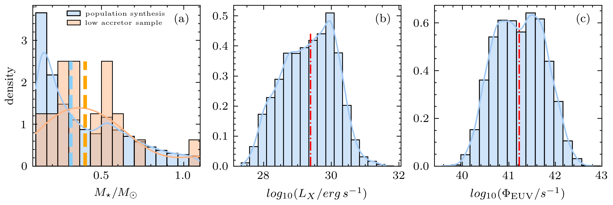
Figure 1: Panel a: histogram of the stellar mass distribution in our population synthesis (in blue) compared with the one from the sample of T23 in orange, where the KDE is overplotted with a solid blue and orange line respectively, and the median value ($0.3$ M_⊙) is marked with a dashed blue line for our sample and with a dashed orange line for the observed sample ($0.4$ M_⊙). Panel b: histogram of the X-ray luminosity density distribution in the X-ray population synthesis, where the KDE is overplotted with a blue solid line and the median value of $29.4$ is marked with a dotted dashed red line. Panel c: histogram of the ionizing flux density distribution in the EUV population synthesis, where the KDE is overplotted with a blue solid line and the median value of $41.2$ is marked with a dotted dashed red line.

We use the one-dimensional viscous evolution code SPOCK (Ercolano & Rosotti, 2015) which evolves the gas following

$$\frac{\partial{\Sigma}}{\partial{t}}=\frac{1}{R}\frac{\partial}{\partial{R}}\left[3R^{1/2}\frac{\partial}{\partial{R}}(\nu\Sigma R^{1/2})\right]-\dot{\Sigma}_{w}(R,t)\,,$$ (1)

where the first term on the right hand side describes the viscous disc evolution (Lynden-Bell & Pringle, 1974), and the second one is a sink term modelling the mass-loss due to internal disc photoevaporation.

We consider either an EUV, FUV, or X-ray mass-loss rate internal photoevaporation profile as they are well-studied in the literature, and simple 1D prescriptions of the disc mass-loss rates are provided.

2.1 X-ray photoevaporation

The X-ray surface mass-loss rate is given following equations 2 and 3 of Picogna et al. (2019), with the parameters for the different stellar masses being provided in Table 1 of Picogna et al. (2021). The mass-loss rate as a function of X-ray luminosity and stellar mass can be described by (Ercolano et al., 2021; Picogna et al., 2021)

$$\dot{M}_{\mathrm{XEUV}}(M_{\star},L_{X,\mathrm{soft}})=\dot{M}_{\mathrm{XEUV}}(M_{\star})\frac{\dot{M}_{\mathrm{XEUV}}(L_{X,\mathrm{soft}})}{\dot{M}_{\mathrm{XEUV}}(L_{X,\mathrm{soft,mean}})}\,,$$ (2)

where the mass-loss rate as a function of stellar mass is

$$\dot{M}_{\mathrm{XEUV}}(M_{\star})=3.93\times 10^{-8}\left(\frac{M_{\star}}{M_{\odot}}\right)$$ (3)

and the dependence on the soft component of the X-ray luminosity is given by

$$\dot{M}_{\mathrm{XEUV}}(L_{X,\mathrm{soft}})=10^{a_{L}\exp{\left(\frac{(\ln(\log(L_{X,\mathrm{soft}})-b_{L})^{2}}{c_{L}}\right)+d_{L}}}\,,$$ (4)

with $a_{L}=-1.947\cdot 10^{17}$, $b_{L}=-1.572\cdot 10^{-4}$, $c_{L}=-0.2866$, $d_{L}=-6.694$. The soft component of the X-ray luminosity is given by

$$L_{X,\mathrm{soft}}=10^{0.95\log{(L_{X})}+1.19}\,,$$ (5)

and was obtained by performing a linear fit between the nominal and soft X-ray luminosities listed in Table 4 of Ercolano et al. (2021). The mean component of the X-ray luminosity is the soft X-ray luminosity $L_{X,\mathrm{soft,mean}}$ of a star with a total X-ray luminosity given by the observational relation between stellar mass and X-ray luminosity (see eq. 15, Güdel et al., 2007).

2.2 EUV photoevaporation

We divided the EUV surface mass-loss rate in its diffuse and direct components following Alexander & Armitage (2007):

$$\dot{\Sigma}_{\mathrm{EUV}}(R)=\dot{\Sigma}_{\mathrm{diffuse}}(R)+\dot{\Sigma}_{\mathrm{direct}}(R,t)\cdot f(R)\,,$$ (6)

where $f(R)=1+\exp{(-\frac{R-R_{\mathrm{in}}}{H_{\mathrm{in}}})}$ is a smoothing function to avoid numerical problems close to the disc inner edge, $R_{\mathrm{in}}(t)$ is the radius of the inner disc edge and $H_{\mathrm{in}}(t)$ is the disc scale height at the inner edge.

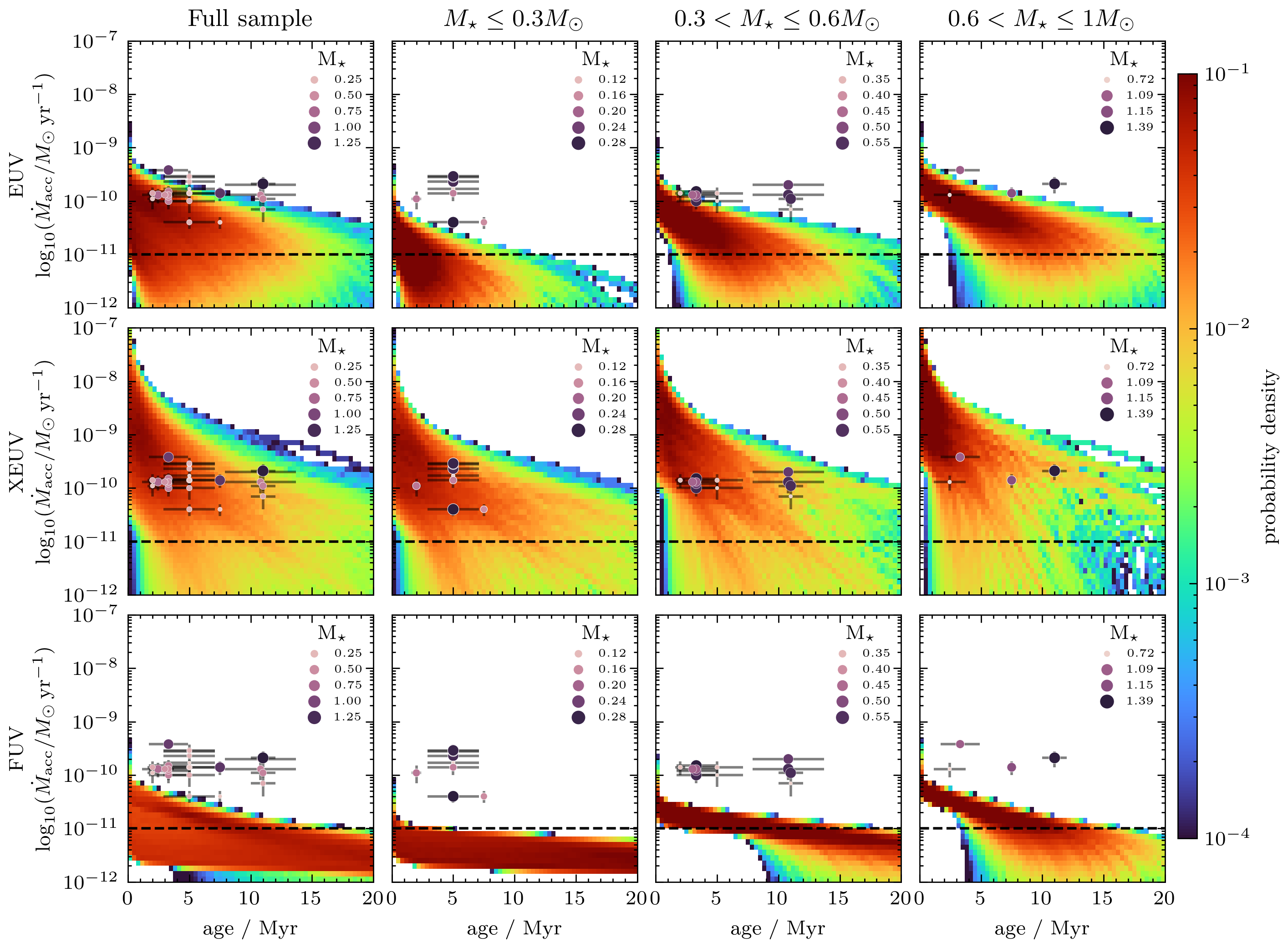
Figure 2: Synthetic populations showing the accretion rates as a function of age. The color mapping shows the probability of finding an object of a given age accreting at a given accretion rate (see text for details). Top row: discs are dispersed by EUV photoevaporation; bottom row: discs are dispersed by X-ray photoevaporation. The first column shows the full stellar mass sample, while the following columns show the result divided in three different stellar mass bins. The low-accretors population of T23 is overplotted with dots with variable size increasing by their stellar mass.

The diffuse component of the EUV surface mass-loss rate is then given by

$$\dot{\Sigma}_{\mathrm{diffuse}}(R)=2n_{0}(R)u_{l}(R)\mu m_{H}\\ \mathrm{for}\ R\geq 0.1R_{g}\,,$$ (7)

where the density at the base of the flow is

$$n_{0}(R)=C_{1}\left(\frac{3\Phi_{\mathrm{diff}}}{4\pi\alpha_{B}R_{g}^{3}}\right)^{1/2}\left(\frac{2}{(R/R_{g})^{15/2}+(R/R_{g})^{25/2}}\right)^{1/5}\,,$$ (8)

the wind launch velocity

$$u_{l}(R)=c_{s}A\exp{\left[B\left(\frac{R}{R_{g}}-0.1\right)\right]}\left(\frac{R}{R_{g}}-0.1\right)^{D}\,,$$ (9)

$\mu=1.35$ the mean molecular weight of the ionized gas, $m_{H}$ the mass of a hydrogen atom, $C_{1}\simeq 0.14$, $R_{g}$ the gravitational radius, $\alpha_{B}=2.6\cdot 10^{-13}$ is the Case B recombination coefficient for atomic hydrogen at $10^{4}$ K, $c_{s}=10$ km $\mathrm{s}^{-1}$ the sound speed of the ionized gas, $A=0.3423$, $B=0.3612$, $D=0.2457$, and the stellar diffuse ionizing EUV flux

$$\Phi_{\mathrm{diff}}=\begin{cases}\Phi_{\mathrm{EUV}}\left(\frac{R_{\mathrm{thin}}}{R_{\mathrm{in}}}\right)&\text{if }R_{\mathrm{thin}}<R_{\mathrm{crit}},\\ \Phi_{\mathrm{EUV}}&\text{otherwise},\end{cases}$$ (10)

where $\Phi_{\mathrm{EUV}}$ is the unattenuated stellar ionizing EUV flux (in photons s^-1), $R_{\mathrm{thin}}$ is the radius at which the disc becomes optically thin in the vertical direction

$$\Sigma_{g}(R_{\mathrm{thin}})=m_{H}\sigma_{\mathrm{13.6\,eV}}^{-1}\,,$$ (11)

$\sigma_{\mathrm{13.6\,eV}}=6.3\cdot 10^{-18}$ cm² is the absorption cross-section for ionizing photons, $R_{\mathrm{crit}}$ is the critical radius at which the gap opens

$$R_{\mathrm{crit}}=1.4\left(\frac{M_{\star}}{M_{\odot}}\right)\ \text{au}\,.$$ (12)

The direct component of the EUV surface mass-loss rate (defined only for $R>R_{\mathrm{in}}$) is given by

$$\dot{\Sigma}_{\mathrm{direct}}(R,t)=2C_{2}\mu m_{H}c_{s}\left[\frac{\Phi_{\mathrm{EUV}}}{4\pi\alpha_{B}(H/R)R_{\mathrm{in}}^{3}(t)}\right]^{1/2}\left[\frac{R}{R_{\mathrm{in}}(t)}\right]^{-a}\,,$$ (13)

where $C_{2}=0.235$, $a=2.42$, $H/R$ is the disc aspect ratio.

2.3 FUV photoevaporation

The combined X-ray/FUV component of the surface mass-loss rate has been defined in eq. A1 of Komaki et al. (2021) with coefficients from their Table 2 (as a function of stellar mass) and their Table 3 (as a function of X-ray/FUV luminosities). However, since in their prescription the FUV contribution is significantly more important than the X-ray one, we assume here a fixed X-ray luminosity and consider only the variation of the FUV component. To simplify the implementation we considered here only the coefficients for a 1 Solar mass star with varying FUV luminosities, and scale then the total mass-loss rate as a function of stellar mass by (Komaki et al., 2021)

$$\dot{M}_{\mathrm{FUV}}\propto\left(\frac{M_{\star}}{M_{\odot}}\right)^{2.06}\,.$$ (14)

2.4 Population synthesis

We assume an initial stellar mass function following Kroupa (2001), $\xi(m)\propto m^{-\alpha}$ , where $\alpha=1.3\pm 0.5$ for $0.08\leq m/M_{\odot}<0.5$ and $\alpha=2.3\pm 0.3$ for $0.5\leq m/M_{\odot}\leq 1$, from which we obtain the distribution shown in Figure 1 (a) for a sample of 10,000 stars with a median value of $\sim 0.3$ M_⊙. The population of observed low accretors from T23 is overplotted in orange, where one can see that the distribution is significantly different from the adopted one due to the low number statistics (24 sources), but the mean of the distribution ($0.4$ M_⊙, shown with a black dashed line) is consistent with the adopted sample.

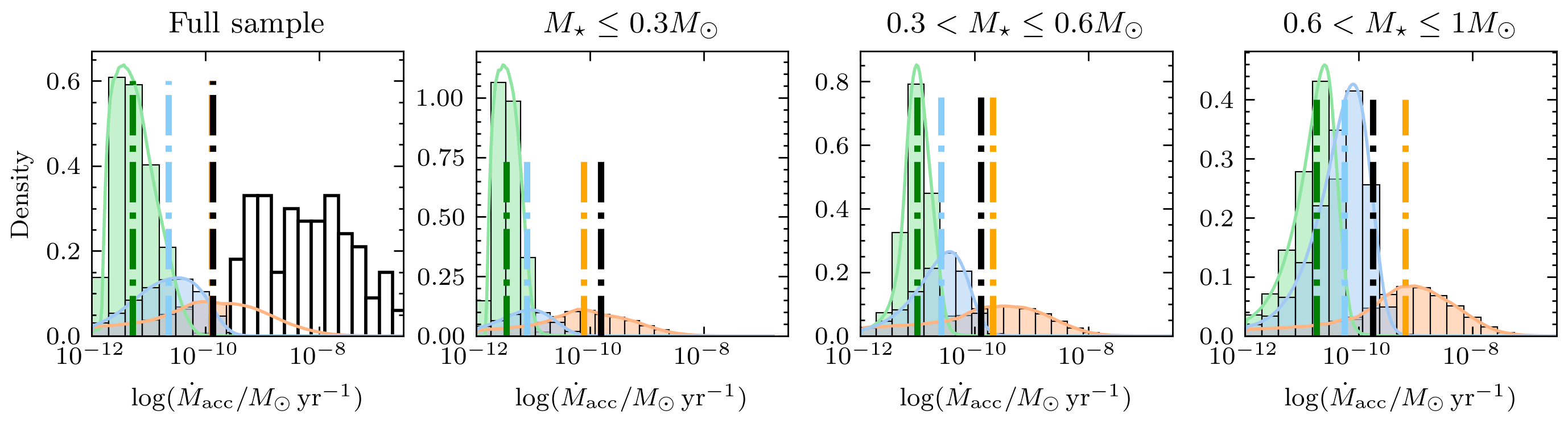
Figure 3: Histogram of the accretion rate density distribution in the EUV (blue), X-ray (orange), and FUV (green) population synthesis. The KDE is overplotted with a solid line for each distribution, and the median values are plotted with dotted-dashed lines. For direct comparison the median accretion rate of the low-accretors population is plotted with a black dotted-dashed line. The distribution of accretion rates from the sample of Manara et al. (2023) is added with a black histogram in the full sample for comparison.

Güdel et al. (2007) derived an observational relation between the median X-ray luminosities and stellar masses

$$\log_{10}(L_{X})=(1.54\pm 0.12)\log_{10}(M_{\star})+(30.31\mp 0.06)\,,$$ (15)

though a large spread is observed around the mean values, which becomes larger for small mass stars (e.g. Getman et al., 2022). Kuhn & Hillenbrand (2019) took a subsample of the Chandra Orion Ultradeep Project (COUP, cf. Getman et al., 2005) and stratified it in three stellar mass bins using the Baraffe et al. (1998) evolutionary models. From this sample one can derive an X-ray luminosity function (XLF) as a function of stellar mass. We then calculated the median stellar mass for the three stellar mass bins given the adopted IMF, and shifted the XLF distribution to match the given value of the stellar mass. We then sampled the X-ray luminosity given the probability density corrected for the stellar mass and obtained the X-ray luminosity distribution shown in Figure 1(b) from the 10,000 sampled stellar masses, with a median value of $10^{29.4}$ erg s^-1 and a spread over four orders of magnitude.

The EUV rates are shown to scale with the ratio of incoming ionising flux. Assuming a chromospheric origins of the EUV flux, we can then adopt the same scaling relation as eq. 15

$$\log_{10}(\Phi_{EUV})=1.54\log_{10}(M_{\star})+42\,$$ (16)

and consider a small dispersion around the mean value for each stellar mass of 0.25 dex, as shown in Figure 1 (c), which gives ionizing fluxes ranging from $10^{40}\,\mathrm{s^{-1}}$ to $10^{42.5}\,\mathrm{s^{-1}}$ with a median of $10^{41.2}\,\mathrm{s^{-1}}$.

Contributions to the FUV luminosity ($L_{\mathrm{FUV}}$) are believed to come both from the activity in the chromosphere ($L_{\mathrm{FUV,chr}}$) and accretion hotspots on the stellar surface (see e.g. Gorti et al., 2009, $L_{\mathrm{FUV,acc}}$). The accretion component, that is more important in the early stages of evolution, can be expressed as

$$L_{\mathrm{FUV,acc}}=10^{-2}\left(\frac{M_{\star}}{M_{\odot}}\right)\left(\frac{R_{\star}}{R_{\odot}}\right)^{-1}\left(\frac{\dot{M}_{\mathrm{acc}}}{10^{-8}\ \mathrm{M}_{\odot}\mathrm{yr}^{-1}}\right)\ \mathrm{L}_{\odot}\,,$$ (17)

assuming the accretion luminosity as a black-body with $T=9000$ K which has a fraction of $4\%$ in the FUV band (Gorti et al., 2009). The chromospheric component of the FUV flux is given by

$$L_{\mathrm{FUV,chr}}=10^{-3.3}L_{\star}\,,$$ (18)

obtained for non-accreting, weak-line T Tauri stars (Valenti et al., 2003).

We constrained the disc properties in order to match the observed mean disc lifetime of 2-3 Myr (see e.g. Ribas et al., 2014). For the EUV profile we sampled the viscous $\alpha$-parameter and scaling radius $R_{1}$ for disc masses ranging from $0.01$–$0.1M_{\star}$ for a typical star with median values from our distribution ($M_{\star}=0.3M_{\odot}$, $\Phi_{\mathrm{EUV}}=10^{41.2}$ s^-1) and then we selected those returning a disc life-time in agreement with observations and obtained a best linear fit given by:

$$R_{1}=60.4\log_{10}({\alpha})+3009.7M_{d}[M_{\star}]+226.6\\ \text{[au]}\,.$$ (19)

We then sampled the whole stellar mass range and obtained the full sampling of the parameter space. For the FUV profile, we did the same procedure, finding a new best fit:

$$\alpha=10^{-9.41+1.678\log_{10}(R_{1})-1.211\log_{10}(M_{d}[M_{\star}])}\,.$$ (20)

For the X-ray profile, the disc evolution is primarily driven by the internal photoevaporation rather than the disc properties, thus we sample uniformly the parameter space fixing only the disc mass to $0.1M_{\star}$, which is reasonable for non self-gravitating discs. We summarize the probed parameter space in Table 1.

Table 1: Parameters for the population synthesis calculations.

Name	Viscosity	$R_{1}$	Disc mass	Stellar mass	Stellar flux
	$\log_{10}(\alpha)$	au	$M_{\star}$	$M_{\odot}$	$(\Phi,\ L_{X})$
EUV	eq. 19	eq. 19	eq. 19	Fig. 1 (a)	Fig. 1 (c)
X	[-4, -2]	[10, 100]	0.1	Fig. 1 (a)	Fig. 1 (b)
FUV	eq. 20	eq. 20	eq. 20	Fig. 1 (a)	variable

3 Results

Figure 2 shows the accretion rates as a function of time for a population synthesis of 10,000 discs sampled as described in Section 2. Overplotted with dots of variable size (based on their stellar mass) is the population of low accretors from T23, and the observational limit of the He I $\lambda 10830$ marked with a black dashed line at $10^{-11}$ M_⊙ yr^-1. From the full sample, shown in the first column, one can immediately see that while the population of discs with the X-ray profile (second row) catches all the observed data points in the region with high density ($>10^{-2}$), the populations using the EUV and FUV photoevaporation profiles (first and last row) cannot explain the data for the older star-forming regions (Orion OB1a and Upper Sco). Furthermore the observational data points lie in the upper region of the distribution, even though they should be a sample of the population accreting at the lowest possible rates. This means that the bulk of the discs in the studied star forming regions covers a region not explained by the EUV or FUV photoevaporation profiles.

Low-mass stars (small dots) cover the lower part of the high density distribution while higher-mass stars the top part. This is expected from the observationally derived relation between accretion rate and stellar masses, that shows a sharp increase of the accretion rate as a function of stellar mass ($\dot{M}$-$M_{*}$) with a broken power law (e.g. Alcalá et al., 2017). Ercolano et al. (2014) proposed that the $\dot{M}$-$M_{*}$ distribution is also a consequence of discs being dispersed by X-ray photoevaporation, which fits well in this overall picture.

In Figure 3 we plot the histogram of the accretion rate distribution for the EUV (in blue) and X-ray (in orange) populations. Overplotted are the median accretion rates in dotted-dashed blue and orange lines respectively, and the median accretion rate for the observed population of low-accretors with a dotted-dashed black line. From this one can directly visualise how the median of the X-ray photoevaporating population and the observed low-accretors is very similar. On the other hand, for the population dispersing via EUV-photoevaporation the median accretion rate of the low-accretors population is close to the high-accretor wing of the EUV population, which is in tension with the observation that the observed objects should represent the lowest end of the mass accretion rate distribution.

Overplotted in Figure 3 (black hystogram) is the observed distribution of accretion rates from the sample of Manara et al. (2023) recently reported by Alexander et al. (2023). Our results show that the observations favour X-ray photoevaporation as the main dispersal mechanism over other models, as it represents well the low-accretor population.

We finally compared the distribution of disc fractions as a function of age, calculated as the time at which the accretion rate drops below the observational limit quoted by T23 ($10^{-11}$ M_⊙ yr^-1) in our population synthesis with the observed distribution of disc fraction (Figure 4, black lines). The EUV and X-ray distributions fit the observational data points perfectly by construction, as we choose the parameter space in order to fit them for the median stellar mass and EUV ionising field. The FUV distribution fits less well the observed population as the stellar luminosity (and thus the wind mass-loss rate) evolves with time (see eq. 17) inducing a stronger stellar mass dependance. The main difference between the models is the parameter space adopted to match the observations which is much more limited for the EUV and FUV profiles with respect to the X-ray one (see Table. 1).

3.1 Mass dependent results

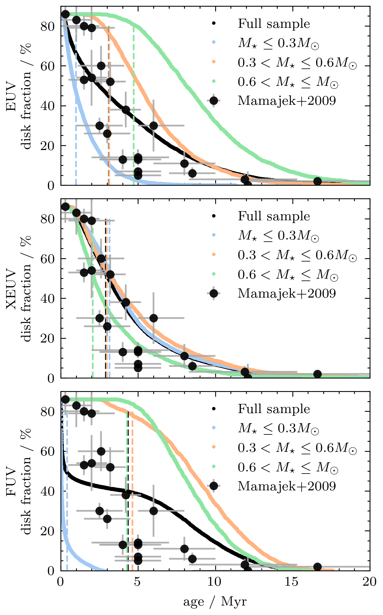
Figure 4: Disc fraction as a function of disc lifetime for the EUV (top panel), X-ray (middle panel) and FUV (bottom panel) synthetic populations compared with the observational data from Mamajek (2009), divided in three stellar mass bins. The median disc life-time increases with stellar mass for the EUV and FUV models, while it decreases for the X-ray models.

The results shown in the previous section assume a well-sampled IMF, which implies that objects at the lower end of the mass range are the most abundant. However the sample of low accretors from T23 includes objects with masses ranging between $0.1$ and $1.39$ M_⊙ and a mean of $0.4$ M_⊙, resulting in a slightly different stellar mass function with respect to the adopted IMF (see Figure 1, a). Despite the low number of objects in observational sample it is worth trying to decouple the effect of stellar mass from the analysis. To this aim we repeat the analysis for separate mass bins, as shown in columns 2 to 4 of Figures 2 and 3. The observed median of the observed accretion rate distribution is always close the median or the lower end of distribution predicted by the X-ray model. For the EUV and FUV distributions, in contrast, the median is always close to the higher end of the predicted distribution, for all mass bins, implying that the EUV and FUV models predict that objects with accretion rates one or two order of magnitude lower than observed should be more common.

Finally, in Figure 4 we explore the effect of stellar mass on the disc lifetimes. In the top panel the population with the X-ray profile profile shows little variation as a function of stellar mass, with a trend of decreasing lifetimes for increasing stellar masses, which is consistent with current observations (Ribas et al., 2015). In the bottom panel, the population with the EUV profile shows a much stronger dependence on the stellar mass, with an inverse trend of decreasing disc lifetime for smaller mass stars. The overall distribution in this case fits the observational data because of the adopted IMF, but it would overpredict the disc fractions for the stellar mass distribution studied in T23.

4 Conclusions

We conducted a population synthesis study of viscously evolving discs subjected to different photoevaporation prescriptions, in order to test these models against the recently published observations of the lowest accretion rates measured by T23. For the case of X-ray photoevaporation the probability of finding an object at a given accretion rate changes as a function of age of the population. However for objects older than approximately 1 Myr it is clearly not improbable to find objects at rates of order $10^{-10}M_{\odot}/yr$. In particular for objects older than about 5 Myr the probability distribution peaks indeed at these values. For lower accretion rates the probabilty decreases sharply for all ages, indicating that the lowest accretors of a population of discs being dissipated by X-ray photoevaporation is indeed expected to be observed accreting at rates of order $10^{-10}M_{\odot}/yr$.

Our findings can be synthesised as follows:

• EUV, FUV and X-ray photoevaporation predict objects with accretion rates as those observed in the low-accretor sample of T23.

• However, the low-accretors are part of the bulk or lower end of the distribution predicted by X-ray photoevaporation, while they fall in the upper end of the EUV and FUV driven populations, which thus would predict an overabundance of objects accreting at significantly lower rates, which is not observed.

• The constraints required by EUV and FUV internal photoevaporation to explain the observed disk lifetime are considerably more stringent than those of X-ray-driven disc evolution (see eq. 19).

• The relationship between disk fraction and stellar mass exhibits a strong dependence for EUV and in particular for FUV profiles, in contradiction with the observed low-accretor population that shows similar accretion rates across a wide range of stellar masses.

• The observed distribution of accretion rates favours X-ray photoevaporation as the main dispersal mechanism.

In light of the results of the population synthesis models shown here, we conclude that the recent low-accretor observations point to X-ray photoevaporation as driving the final stages of disc dispersal.

Data Availability

The data for the population synthesis calculations is available at https://github.com/GiovanniPicogna/low-accretors

References

- Alcalá et al. (2017) Alcalá J. M., et al., 2017, A&A, 600, A20
- Alexander & Armitage (2007) Alexander R. D., Armitage P. J., 2007, MNRAS, 375, 500
- Alexander & Pascucci (2012) Alexander R. D., Pascucci I., 2012, MNRAS, 422, L82
- Alexander et al. (2006) Alexander R. D., Clarke C. J., Pringle J. E., 2006, MNRAS, 369, 229
- Alexander et al. (2023) Alexander R., Rosotti G., Armitage P. J., Herczeg G. J., Manara C. F., Tabone B., 2023, MNRAS, 524, 3948
- Baraffe et al. (1998) Baraffe I., Chabrier G., Allard F., Hauschildt P. H., 1998, A&A, 337, 403
- Carrera et al. (2017) Carrera D., Gorti U., Johansen A., Davies M. B., 2017, ApJ, 839, 16
- Ercolano & Owen (2016) Ercolano B., Owen J. E., 2016, MNRAS, 460, 3472
- Ercolano & Pascucci (2017) Ercolano B., Pascucci I., 2017, Royal Society Open Science, 4, 170114
- Ercolano & Picogna (2022) Ercolano B., Picogna G., 2022, European Physical Journal Plus, 137, 1357
- Ercolano & Rosotti (2015) Ercolano B., Rosotti G., 2015, MNRAS, 450, 3008
- Ercolano et al. (2014) Ercolano B., Mayr D., Owen J. E., Rosotti G., Manara C. F., 2014, MNRAS, 439, 256
- Ercolano et al. (2017a) Ercolano B., Rosotti G. P., Picogna G., Testi L., 2017a, MNRAS, 464, L95
- Ercolano et al. (2017b) Ercolano B., Jennings J., Rosotti G., Birnstiel T., 2017b, MNRAS, 472, 4117
- Ercolano et al. (2021) Ercolano B., Picogna G., Monsch K., Drake J. J., Preibisch T., 2021, MNRAS, 508, 1675
- Getman et al. (2005) Getman K. V., et al., 2005, ApJS, 160, 319
- Getman et al. (2022) Getman K. V., Feigelson E. D., Garmire G. P., Broos P. S., Kuhn M. A., Preibisch T., Airapetian V. S., 2022, ApJ, 935, 43
- Gorti et al. (2009) Gorti U., Dullemond C. P., Hollenbach D., 2009, ApJ, 705, 1237
- Güdel et al. (2007) Güdel M., et al., 2007, A&A, 468, 353
- Jennings et al. (2018) Jennings J., Ercolano B., Rosotti G. P., 2018, MNRAS, 477, 4131
- Komaki et al. (2021) Komaki A., Nakatani R., Yoshida N., 2021, ApJ, 910, 51
- Kroupa (2001) Kroupa P., 2001, MNRAS, 322, 231
- Kuhn & Hillenbrand (2019) Kuhn M. A., Hillenbrand L. A., 2019, ApJ, 883, 117
- Lesur et al. (2022) Lesur G., et al., 2022, arXiv e-prints, p. arXiv:2203.09821
- Lynden-Bell & Pringle (1974) Lynden-Bell D., Pringle J. E., 1974, MNRAS, 168, 603
- Mamajek (2009) Mamajek E. E., 2009, in Usuda T., Tamura M., Ishii M., eds, American Institute of Physics Conference Series Vol. 1158, Exoplanets and Disks: Their Formation and Diversity. pp 3–10 (arXiv:0906.5011), doi:10.1063/1.3215910
- Manara et al. (2023) Manara C. F., Ansdell M., Rosotti G. P., Hughes A. M., Armitage P. J., Lodato G., Williams J. P., 2023, in Inutsuka S., Aikawa Y., Muto T., Tomida K., Tamura M., eds, Astronomical Society of the Pacific Conference Series Vol. 534, Astronomical Society of the Pacific Conference Series. p. 539 (arXiv:2203.09930), doi:10.48550/arXiv.2203.09930
- Monsch et al. (2019) Monsch K., Ercolano B., Picogna G., Preibisch T., Rau M. M., 2019, MNRAS, 483, 3448
- Pascucci et al. (2022) Pascucci I., Cabrit S., Edwards S., Gorti U., Gressel O., Suzuki T., 2022, arXiv e-prints, p. arXiv:2203.10068
- Picogna et al. (2019) Picogna G., Ercolano B., Owen J. E., Weber M. L., 2019, MNRAS, 487, 691
- Picogna et al. (2021) Picogna G., Ercolano B., Espaillat C. C., 2021, MNRAS, 508, 3611
- Ribas et al. (2014) Ribas Á., Merín B., Bouy H., Maud L. T., 2014, A&A, 561, A54
- Ribas et al. (2015) Ribas Á., Bouy H., Merín B., 2015, A&A, 576, A52
- Thanathibodee et al. (2022) Thanathibodee T., Calvet N., Hernández J., Maucó K., Briceño C., 2022, AJ, 163, 74
- Thanathibodee et al. (2023) Thanathibodee T., Molina B., Serna J., Calvet N., Hernández J., Muzerolle J., Franco-Hernández R., 2023, ApJ, 944, 90
- Valenti et al. (2003) Valenti J. A., Fallon A. A., Johns-Krull C. M., 2003, VizieR Online Data Catalog, p. J/ApJS/147/305
- Weber et al. (2020) Weber M. L., Ercolano B., Picogna G., Hartmann L., Rodenkirch P. J., 2020, MNRAS, 496, 223