Implicit Obstacle Map-driven Indoor Navigation Model for Robust Obstacle Avoidance

Abstract.

Robust obstacle avoidance is one of the critical steps for successful goal-driven indoor navigation tasks. Due to the obstacle missing in the visual image and the possible missed detection issue, visual image-based obstacle avoidance techniques still suffer from unsatisfactory robustness. To mitigate it, in this paper, we propose a novel implicit obstacle map-driven indoor navigation framework for robust obstacle avoidance, where an implicit obstacle map is learned based on the historical trial-and-error experience rather than the visual image. In order to further improve the navigation efficiency, a non-local target memory aggregation module is designed to leverage a non-local network to model the intrinsic relationship between the target semantic and the target orientation clues during the navigation process so as to mine the most target-correlated object clues for the navigation decision. Extensive experimental results on AI2-Thor and RoboTHOR benchmarks verify the excellent obstacle avoidance and navigation efficiency of our proposed method. The core source code is available at https://github.co
m/xwaiyy123/object-navigation.

1. Introduction

Indoor goal-driven navigation task is a vital task in computer vision and has been widely used in various real-world applications, such as  (Li et al., 2021; Chaplot et al., 2020; Luo et al., 2022). Given a predetermined target object, the objective of the navigation task is to enable the agent to automatically locate the target object in unseen indoor settings (Zhang et al., 2021; Du et al., 2020b; Dang et al., 2022a). Benefiting from the development of the reinforcement learning (RL), most navigation models focus on leveraging RL technique to realize the auto-navigation in a trial-and-error manner. Taking a sequence of RGB images obtained during the agent’s interaction with the environment as input, a policy network is trained to generate a series of actions that direct the agent toward the target object. However, due to unknown spatial layout and strong noise interference lying in the unseen scenes, robust indoor goal-driven navigation is still a challenging task.

The popular object navigation models can be categorized into two primary approaches: end-to-end navigation (Fukushima et al., 2022; Du et al., 2020a; Ye and Yang, 2021) and BEV (bird’s-eye view) semantics-based navigation (Chaplot et al., 2019, 2020). End-to-end navigation methods aim to learn reactive motion decisions based on the perceived environmental information, whereas BEV semantics-based navigation methods focus on utilizing the gathered scene information to construct a BEV (bird’s-eye view) scene map for route planning. Despite their effectiveness, these methods still struggle to achieve robust obstacle perception (e.g., table and wall) during the navigation process. Consequently, the agent is prone to get “stuck” (becoming immobilized) in a local area, ultimately resulting in navigation failure. For instance, if the obstacle distribution around the agent is not included in the image or the model does not recognize the obstacle information in the image, the model might erroneously believe that there are no obstacles in the current direction and repeatedly performs incorrect motion actions, leading to immobilization. Figure 1 depicts a typical scenario where the agent has identified the target object, namely garbage, but the obstacle, i.e., a table, is not included in the image. The agent presumes that it can approach the target object by moving forward, and repeatedly performs “moveforward” actions (as seen in $step_{7}\sim step_{10}$), leading to it getting stuck at its current position.

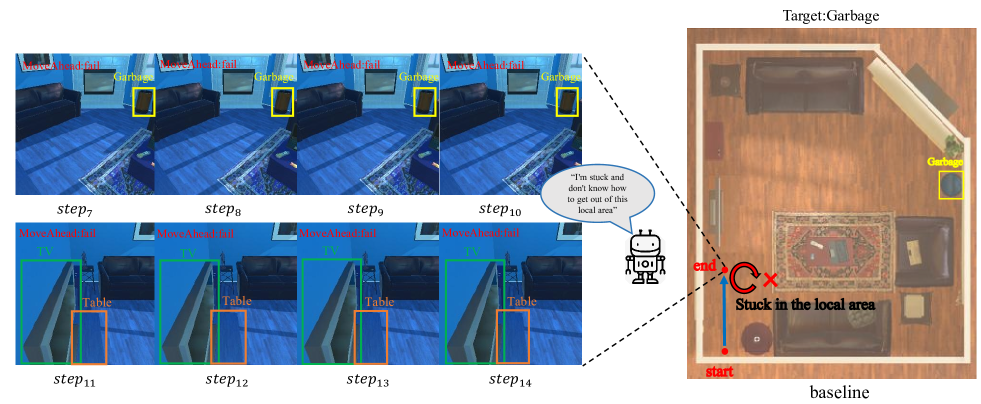
Figure 1. These consecutive frames are selected from an episode, no the obstacle is included in $\boldsymbol{step}_{7}\sim\boldsymbol{step}_{10}$, the agent believes it can move forward, and does not understand the obstacle distribution in $\boldsymbol{step}_{11}\sim\boldsymbol{step}_{14}$, which still believes that it can move forward.

To mitigate it, in this paper, we propose a novel and effective implicit obstacle map-driven indoor object navigation framework for robust obstacle avoidance during navigation process. By encoding “passable” or “impassable” direction as the obstacle distribution, the navigation model is expected to precisely recognize the surrounding obstacles so as to help agent choose the correct direction and escape from these obstacles. Specifically, our framework consists of two modules, i.e., an implicit obstacle map module and a non-local target memory aggregation module. In the implicit obstacle map module, it aims to learn an implicit layout representation that describes the potential obstacle distribution in the local area around the agent through trial-and-error. In detail, during the navigation process, when an obstacle is touched in the agent’s forward direction, the current direction is impassable and would be encoded as a “impassable” vector representation. Conversely, if no obstacle is touched, the current direction is passable and thus encoded as a “passable” vector representation. By aggregating these historical “impassable” and “passable” vector representations with an MLP network, we can learn an implicit representation about the potential obstacle layout around the agent for obstacle perception. Compared to previous visual image-based obstacle identification, our trial-and-error obstacle perception presents significant robustness to obstacle missing in the image or the issue of detection failure. In order to further accelerate the approaching speed of the agent towards the target object, the non-local target memory aggregation module employs a non-local module to conduct cross-attention between the target semantic and the collected target orientation clues during the navigation process. As such, the vital object clues that are highly correlated with the target object would be mined for navigation decisions, thereby significantly improving the navigation efficiency (that is reducing the path length).

To summarize, our main contributions are as follows:

1) We propose a novel implicit obstacle map-enhanced navigation framework for robust obstacle avoidance, where the implicit obstacle map is generated through a trial-and-error mechanism, presenting a significant advantage in robustness over the conventional visual image-based obstacle recognition methods.

2) To further improve the navigation efficiency, a non-local target memory aggregation module is proposed to mine the vital target object clues for navigation decisions through the cross-attention mechanism between the target orientation clues and the target semantic.

3) Extensive experimental results on AI2-Thor and RoboTHOR benchmarks verify our significant navigation advantages, in terms of the success ratio and efficiency, over previous methods.

2. Related works

The indoor goal-driven navigation model mainly consists of two parts, namely the feature extractor and policy network, the continuous improvement of these two parts has greatly improved the performance of the navigation model.

The image feature contains a lot of spatial layout information, so the end-to-end navigation model can be built by using the image feature (Zhu et al., 2017; Mayo et al., 2021; Gadre et al., 2022). A large number of experiments have verified that object feature obtained by object detector plays a key role in improving the performance of the navigation model (Du et al., 2020a), and more methods tend to use object features to construct navigation model (Fukushima et al., 2022; Ramakrishnan et al., 2022; Pal et al., 2021). Du et al. (Du et al., 2020a) and Zhang et al. (Zhang et al., 2021) used the relationship between objects to build graphs, graph feature helps the agent quickly find the target object location, which greatly improves the efficiency of the model. There are many similar methods (Dang et al., 2022a; Yang et al., 2018; Hu et al., 2021; Li et al., 2021; Ye and Yang, 2021; Campari et al., 2020). However, Frequent changes of objects in the agent’s view can destroy the graph structure and affect the stability of the model. Some works (Savinov et al., 2018; Zhu et al., 2019) built memory features to retain some important image features or object features. The transformer (Vaswani et al., 2017; Fukushima et al., 2022; Fang et al., 2019) and the graph (Savinov et al., 2018; Wu et al., 2019) are used to process the memory feature. But using the transformer or graph to process a large number of memory features may lead to a large amount of calculation and the inefficiency of the model. In our method, the size of the memory is limited, and the non-local aggregation with a simple structure is used for the target memory to reduce the amount of calculation and maintain the performance of the model.

The navigation method based on the semantic map (Chaplot et al., 2019) is an idea that combines deep learning with traditional SLAM (Snavely et al., 2008; Izadi et al., 2011). The construction process of semantic map is divided into two steps (Chaplot et al., 2020), the semantic segmentation model (Hu et al., 2019; He et al., 2017; Jiang et al., 2018) segments objects in the image, then both depth image and object semantic are projected to Bird’s Eye View(BEV) to get semantic map. The policy network outputs action distribution to complete obstacle avoidance and navigation only based on the semantic map, this method (Chaplot et al., 2019, 2020; Liang et al., 2021; Ramakrishnan et al., 2022) has a strong dependency on semantic map. However, a large amount of projection error and inaccurate representation of spatial layout results in an imprecise semantic map, which can lead to a decrease in the model performance. The implicit obstacle map we designed can get the obstacle distribution around the agent, its structure is simple, and the computational complexity is small.

Most navigation models combine RNN and Multilayer Perceptron(MLP) to model policy network (Zhu et al., 2017; Wortsman et al., 2019; Mayo et al., 2021; Zhang et al., 2022; Wu et al., 2019). There are also a few works that directly use CNN (Liang et al., 2021; Ye and Yang, 2021) or MLP (Yang et al., 2018) as policy networks. Most of the policy networks are trained by using reinforcement learning, including asynchronous advanced actor critical (Zhang et al., 2021; Zhu et al., 2017; Fukushima et al., 2022; Mnih et al., 2016) (A3C), proximal policy optimization (Maksymets et al., 2021; Schulman et al., 2017)(PPO), and Deep Q-learning (Liang et al., 2021; Ye and Yang, 2021; Mnih et al., 2015). Very few works (Ramakrishnan et al., 2022) use supervised learning to train models. Some models (Du et al., 2020b; Dang et al., 2022a; Du et al., 2020a) are trained using both supervised learning and reinforcement learning. The models based on semantic map (Chaplot et al., 2020; Ramakrishnan et al., 2022; Luo et al., 2022) use the traditional Fast Marching Method (Sethian, 1996) for path planning and don’t need to train.

3. Method

3.1. Problem Setting

In the context of the indoor object navigation task, given an unseen environment and a predetermined target object, the goal-driven indoor navigation method aims to control the moving of the agent so as to reach the spatial position of the target object. We formulate the indoor navigation task as a Markov decision process, consisting of 3 elements: a state set, an action set, and a reward function. The state set: observed RGB image; the action set: $\mathscr{A}=\{MoveAhead;\,RotateLeft;\,RotateRight;\,LookDown;\,LookUp;\\ \,Done\}$. During the navigation process, at each time step, given the current state $\boldsymbol{o}_{\boldsymbol{t}}$ and the target object $\boldsymbol{g}$, the agent makes the action decision $\boldsymbol{a}_{\boldsymbol{t}}$ based on the learned policy network $\pi\left(\boldsymbol{a}_{\boldsymbol{t}}|\boldsymbol{o}_{\boldsymbol{t}},\boldsymbol{g}\right)$ and achieves the corresponding reward $\boldsymbol{r}_{\boldsymbol{t}}$. The RL algorithm aims to learn the optimal navigation decision so as to maximize the rewards for reaching the location of the target object efficiently.

In order to ensure that the agent quickly learns to avoid obstacles and navigate to the target efficiently, we propose two new modules based on the existing feature extraction modules: implicit obstacle map (IOM) and non-local target memory aggregation module (NTMA). The overall structure of the designed model is shown in Figure 2. When the agent interacts with the environment, the image $\boldsymbol{o}_{\boldsymbol{t}}$, the implicit obstacle distribution feature $\boldsymbol{m}_{\boldsymbol{t}}$, and the target orientation feature $\boldsymbol{D}_{\boldsymbol{t}}$ are obtained. The $\boldsymbol{m}_{\boldsymbol{t}}$ and the $\boldsymbol{D}_{\boldsymbol{t}}$ are used to build implicit obstacle map and target memory respectively. Both the implicit obstacle map embedding feature $\boldsymbol{M}_{\boldsymbol{t}}$ and the target memory aggregation embedding feature $\boldsymbol{F}_{\boldsymbol{t}}$ outputed by non-local target memory aggregation are used as state representation $\boldsymbol{s}_{\boldsymbol{t}}$. Concatenating the image feature and object feature $\boldsymbol{i}_{\boldsymbol{t}}$, the policy network outputs the action distribution $\boldsymbol{a}_{\boldsymbol{t}}$ according to the state $\boldsymbol{s}_{\boldsymbol{t}}$.

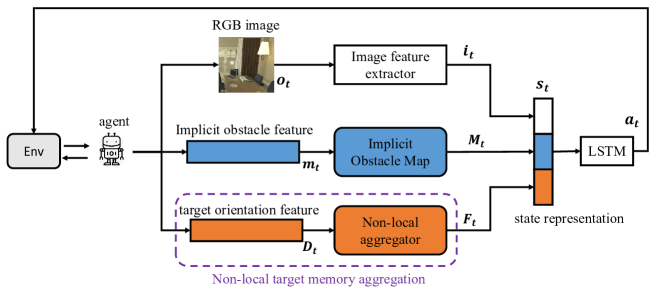
Figure 2. Model overview. The agent obtains RGB image $\boldsymbol{o}_{\boldsymbol{t}}$, implicit obstacle vector feature $\boldsymbol{m}_{\boldsymbol{t}}$, and target orientation feature $\boldsymbol{D}_{\boldsymbol{t}}$ when it interacts with the environment. Image feature extractor outputs image embedding and object feature $\boldsymbol{i}_{\boldsymbol{t}}$ (boundingbox, confidence, etc.) based on the RGB image $\boldsymbol{o}_{\boldsymbol{t}}$. The implicit obstacle distribution feature $\boldsymbol{m}_{\boldsymbol{t}}$ is put into the implicit obstacle map to get the implicit obstacle embedding feature $\boldsymbol{M}_{\boldsymbol{t}}$. The non-local aggregator outputs target orientation embedding feature $\boldsymbol{F}_{\boldsymbol{t}}$ based on the collected target orientation feature $\boldsymbol{D}_{\boldsymbol{t}}$. $\boldsymbol{i}_{\boldsymbol{t}}$, $\boldsymbol{M}_{\boldsymbol{t}}$, and $\boldsymbol{F}_{\boldsymbol{t}}$ are concatenated as the state representation $\boldsymbol{s}_{\boldsymbol{t}}$. Finally, the policy network LSTM outputs the action distribution according to $\boldsymbol{s}_{\boldsymbol{t}}$.

3.2. Implicit obstacle map generation

In the indoor scene, the obstacle distribution around the agent can be implicitly obtained according to the change of the agent’s coordinate when the agent moves forward. Assuming that the navigation model sends a “forward” command at the current moment, if the agent’s coordinate is not changed, there is an obstacle in the agent’s current direction, otherwise, the current direction is passable.

Based on the above characteristic, the implicit obstacle map module is proposed to construct the obstacle distribution around the agent. The working process of implicit obstacle map is shown in Figure 3. For each reachable position, the agent has $8$ forward directions, and every two adjacent directions differ by $45^{\circ}$. $\boldsymbol{z}_{\boldsymbol{t}}\in\mathbb{R}^{1\times 8}$ indicates whether the 8 directions of the current position are passable. The agent is orienting the direction of the red arrow and moves forward.

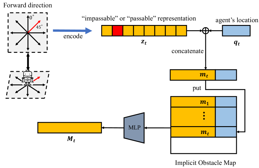
Figure 3. The “impassable” or “passable” representation are encoded as the feature vector $\boldsymbol{z}_{\boldsymbol{t}}$. $\boldsymbol{z}_{\boldsymbol{t}}$ and the agent’s coordinates $\boldsymbol{q}_{\boldsymbol{t}}$ are concatenated to get the implicit obstacle distribution feature $\boldsymbol{m}_{\boldsymbol{t}}$ of the current position. $\boldsymbol{m}_{\boldsymbol{t}}$ is input into the implicit obstacle map. After the implicit obstacle map is extracted by the MLP, the obstacle distribution embedding feature is obtained.

If the agent’s coordinate has not changed, the current direction is impassable, and the corresponding location (red square in Figure 3) of the vector feature $\boldsymbol{z}_{\boldsymbol{t}}$ is set to $-1$, otherwise, it is set to $1$. The other locations of $\boldsymbol{z}_{\boldsymbol{t}}$ are set to $0$. Then the agent’s current coordinate $\boldsymbol{q}_{\boldsymbol{t}}\in\mathbb{R}^{1\times 2}$ and $\boldsymbol{z}_{\boldsymbol{t}}$ are concatenated to construct the implicit obstacle distribution feature $\boldsymbol{m}_{\boldsymbol{t}}\in\mathbb{R}^{1\times 10}$. $\boldsymbol{m}_{\boldsymbol{t}}$ can implicitly represent the obstacle distribution around the agent’s current position, and it is also the basic unit of the implicit obstacle map. If the current direction is passable, $\boldsymbol{m}_{\boldsymbol{t}}$ is put into a fixed-size implicit obstacle map ($\boldsymbol{IOM}\in\mathbb{R}^{e\times 10}$) (The rest is filled with zeros). If the current direction is impassable or the agent’s current location has been reached before (The coordinate is same as the previous position), $\boldsymbol{z}_{\boldsymbol{i}}$ that included in the previous corresponding feature $\boldsymbol{m}_{\boldsymbol{i}}(i\leqslant t-1)$ continues to be encoded. When the number of the previous implicit features $\left\{\boldsymbol{m}_{\boldsymbol{i}}|i\leqslant t-1\right\}$ exceeds $e$, $e$ previous implicit obstacle distribution features $\left\{\boldsymbol{m}_{\boldsymbol{i}}|i\leqslant t-1\right\}$ that are closest to the current implicit obstacle distribution feature $\boldsymbol{m}_{\boldsymbol{t}}$ are retained. The features in the implicit obstacle map is then extracted by two linear layers:

(1) $$\boldsymbol{y_{1}}=\delta_{1}\left(Ln_{1}\left(\boldsymbol{IOM}\right)\right),$$

(2) $$\boldsymbol{y_{2}}=\delta_{2}\left(Ln_{2}\left(\boldsymbol{y}_{\boldsymbol{1}}^{T}\right)\right)^{T},$$

where $\delta_{1}$ and $\delta_{2}$ are activation function $Relu$. $\boldsymbol{y}_{\boldsymbol{1}}\in\mathbb{R}^{e\times 32}$ that has a higher dimension is obtained by the linear layer $Ln_{1}$, which helps the agent better understand the obstacle distribution. The role of $Ln_{2}$ is to compress the size of the implicit obstacle map embedding representation $\boldsymbol{y_{1}}$ so that the policy network can make full use of the feature information in the $\boldsymbol{y_{1}}$. Ultimately, implicit obstacle map embedding representation $\boldsymbol{M_{t}}=\boldsymbol{y_{2}}\in\mathbb{R}^{1\times 32}$ is the embedding representation needed by the policy network. Because $\boldsymbol{M_{t}}$ includes the obstacle distribution information around the current agent, the policy network can output reasonable actions to avoid obstacles according to $\boldsymbol{M_{t}}$.

3.3. Non-local target memory aggregation

The agent completes obstacle avoidance by rotating and moving forward. The insensitivity for target orientation makes the agent choose an unreasonable rotation direction only based on implicit obstacle map, which leads the agent to move away from the target object and creates inefficient navigation. Therefore, inspired by (Dang et al., 2022b), we design a non-local target memory aggregation module. The core idea of the non-local target memory aggregation is to perform a cross-attention between the multiple target orientation features in the target memory and the current target semantic, then target memory is aggregated into a weighted target orientation feature. The weighted target orientation feature provides important target orientation information for the agent.

As shown in Figure 4, for the current state, the target orientation feature $\boldsymbol{D_{t}}\in\mathbb{R}^{1\times 9}$ is obtained by concatenating object feature $\boldsymbol{d_{t}}\in\mathbb{R}^{1\times 5}$ (the bounding box and confidence of the target object) obtained by DETR and the agent’s pose $\boldsymbol{l_{t}}\in\mathbb{R}^{1\times 4}$ (plane coordinate $\boldsymbol{q_{t}}=(x,y)$, yaw angle $\boldsymbol{\theta_{r}}$, pitch angle $\boldsymbol{\theta_{h}}$). The $\boldsymbol{D_{t}}$ is then concatenated with previous target orientation features $\boldsymbol{D_{1}}\sim\boldsymbol{D_{t-1}}$ to construct the target memory $\boldsymbol{T}\in\mathbb{R}^{n\times 9}$, $n\leqslant\tau$ is the number of features currently accumulated, and $\tau$ is the maximum length of $\boldsymbol{T}$. If $n>\tau$, the previous feature $\boldsymbol{D_{i}}$ that is farthest from $\boldsymbol{D_{t}}$ will be discarded. After expanding the dimension by the two layers of MLP, $\boldsymbol{T}$ is converted to $\boldsymbol{\widehat{T}}\in\mathbb{R}^{n\times 32}$. The original target semantic $\boldsymbol{g}\in\mathbb{R}^{1\times k}$ is a one-hot vector ($k$ represents the number of object categories in all scenes). To keep the target semantics consistent with the current scene features, $\boldsymbol{g}$ is transformed into the current target semantic $\boldsymbol{p}\in\mathbb{R}^{1\times 64}$ by another two layers of MLP. The target semantic $\boldsymbol{p}$ is then concatenated with the agent’s pose $\boldsymbol{l_{t}}$ to enhance target semantic $\boldsymbol{p}$ and obtain target semantic feature $\boldsymbol{P}\in\mathbb{R}^{1\times 68}$. After reducing the dimension by the two layers of MLP, $\boldsymbol{P}$ is converted to $\boldsymbol{\widehat{P}}\in\mathbb{R}^{1\times 32}$.

In order to get the important target orientation embedding $\boldsymbol{F_{t}}$, $\boldsymbol{P}$ is treated as query, and $\boldsymbol{\widehat{T}}$ as key and value, which are then input into the non-local network for cross-attention:

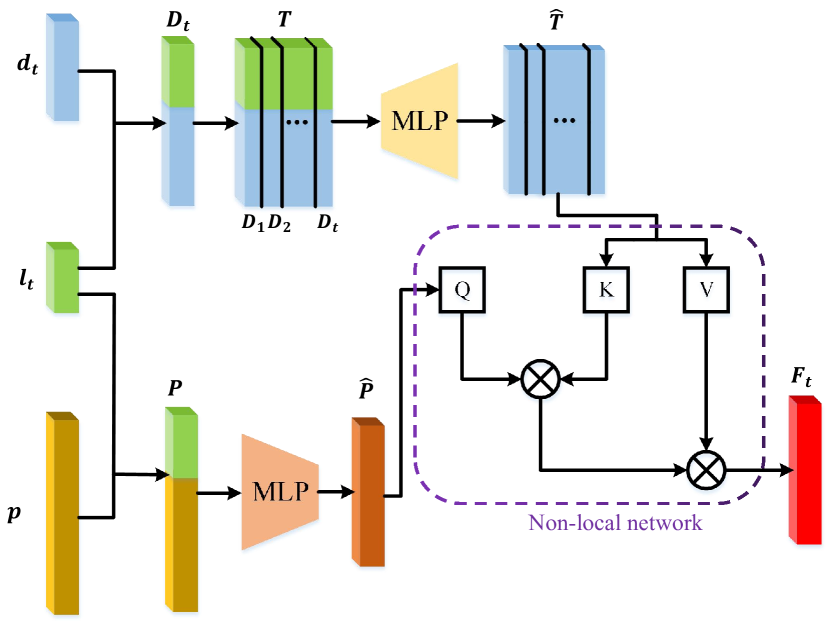
Figure 4. Target orientation features are accumulated to obtain target memory. The target memory feature and target semantic feature perform non-local aggregation to obtain the target orientation embedding feature.

(3) $$\boldsymbol{\widehat{Q}_{i}}=\boldsymbol{\widehat{P}\,\widehat{W}_{i}^{Q}},\,\,\,\boldsymbol{\widehat{K}_{i}}=\boldsymbol{\widehat{T}\,\widehat{W}_{i}^{K}},\,\,\,\,\boldsymbol{\widehat{V}}=\boldsymbol{\widehat{T}\,\widehat{W}^{V}},$$

$$\boldsymbol{\widehat{h}_{i}}=\mathrm{softmax}\left({{\boldsymbol{\widehat{Q}_{i}\widehat{K}_{i}^{T}}}\Bigg{/}{\sqrt{d_{k}}}}\right),\,\,\,\,i=1,2,\cdots,\widehat{Nh},$$

$$\boldsymbol{F_{t}}=cat\left(\boldsymbol{\widehat{h}_{1}},\boldsymbol{\widehat{h}_{2}},\cdots,\boldsymbol{\widehat{h}_{\widehat{Nh}}}\right)\boldsymbol{\widehat{W}^{O}\,\widehat{V}},$$

where $\boldsymbol{\widehat{h}_{i}}$ is the weight that represent which target orientation features are more important for the current target semantic $\boldsymbol{\widehat{P}}$. In $\boldsymbol{\widehat{V}}$, the features that are more correlated with $\boldsymbol{\widehat{P}}$ are assigned larger weights, so that $\boldsymbol{\widehat{h}_{i}}$ is used to weight and sum the features in $\boldsymbol{\widehat{V}}$, and target orientation embedding $\boldsymbol{F_{t}}\in\mathbb{R}^{1\times 32}$ is got by formula 3. Since important target orientation information is included in $\boldsymbol{F_{t}}$, the agent can choose a more reasonable rotation direction based on $\boldsymbol{F_{t}}$ to approach the target faster and improve navigation efficiency.

3.4. Navigation Decision Based on RL

3.4.1. Policy network

In the image feature extraction, the image feature $\boldsymbol{\widehat{i}_{t}}$ output by ResNet(He et al., 2016) and the weighted object feature $\boldsymbol{\widehat{r}_{t}}$(Dang et al., 2022a) output by DETR (Carion et al., 2020) are obtained, and they are adaptively fused with the implicit obstacle map embedding representation $\boldsymbol{M_{t}}$ and target orientation embedding representation $\boldsymbol{F_{t}}$. The state representation $\boldsymbol{s_{t}}$ is then obtained:

(4) $$\boldsymbol{s_{t}}=cat\left(\boldsymbol{\,\widehat{i}_{t}},\boldsymbol{\widehat{r}_{t}},\boldsymbol{M_{t}},\boldsymbol{F_{t}}\right)\boldsymbol{W_{a}}\,,$$

the LSTM(Hochreiter and Schmidhuber, 1997) module is treated as a policy network $\pi\left(\boldsymbol{a_{t}}|\boldsymbol{s_{t}}\right)$, and the asynchronous advantage actor-critic(A3C) algorithm(Mnih et al., 2016) is used to train the navigation model.

3.4.2. Reward Function

We also design a new reward mechanism to extend the positive impact of implicit obstacle map and non-local target memory aggregation on the model, the detail is as follows:

1) -0.01           Penalty reward for each time step;

2) 0.01           The agent does not find the object, and the agent moves forward;

3) 0.01             The agent finds the object, and the distance between the agent and the target decreases;

4) -0.01           The agent collides with an obstacle;

5) 0.02             The agent avoids the obstacle;

6) 5                   Success.

4. Experiment

4.1. Experimental Setting

4.1.1. Dataset.

The AI2-Thor(Kolve et al., 2017) and the RoboTHOR(Deitke et al., 2020) are selected to evaluate the performance of our method. Because their environment layout is very close to the real indoor scene, many works(Yang et al., 2018; Wortsman et al., 2019; Du et al., 2020a; Zhang et al., 2021) use them as the test environment. AI2-Thor includes 4 types of room layouts: kitchen, living room, bedroom, and bathroom, each room layout consists of 30 floorplans, of which 20 rooms are used for training, 5 rooms for validation, and 5 rooms for testing. RoboTHOR consists of 75 scenes, 60 of which are used for training and 15 for validation. The spatial layout of RoboTHOR is more complicated than that of AI2-Thor.

4.1.2. Evaluation Metrics.

Success rate (SR), success weighted by path length (SPL)(Anderson et al., 2018), and success weighted by action efficiency (SAE) (Zhang et al., 2021) metrics are used to evaluate our method. SR is the success rate of the agent in completing the goal-driven navigation task, and its formula is $SR=\frac{1}{K}\sum\nolimits_{i=1}^{K}{Suc_{i}}$, where $K$ is the number of episodes, and $Suc_{i}$ is indicates whether the $i$-th episode is successful. SPL indicates the efficiency of the agent to complete the task in the successful episodes, its formula is $SPL=\frac{1}{K}\sum\nolimits_{i=1}^{K}{Suc_{i}}\frac{L_{i}^{*}}{\max\left(L_{i},L_{i}^{*}\right)}$, where $L_{i}$ is the length of the path actually traveled by the agent. $L_{i}^{*}$ is the optimal path length provided by the simulator. SAE represents the proportion of forward actions in successful episodes, which reflects the efficiency of the agent from another perspective, its formula is $SAE=\frac{1}{K}\sum\nolimits_{i=1}^{K}{Suc_{i}}\frac{\sum\nolimits_{t=0}^{T}{\mathbb{I}\left(a_{t}^{i}\in\mathscr{A}_{change}\right)}}{\sum\nolimits_{t=0}^{T}{\mathbb{I}\left(a_{t}^{i}\in\mathscr{A}_{all}\right)}}$, where $\mathbb{I}$ is the indicator function, $a_{t}^{i}$ is the agent’s action at time $t$ in episode $i$. $\mathscr{A}_{all}$ is action space $\mathscr{A}$ in section 3.1. $\mathscr{A}_{change}$ represents move ahead.

4.1.3. Implementation Details.

Our model is trained by 14 workers on 2 RTX 2080Ti Nvidia GPUs. Similar to the previous method, we first use action label samples for pre-training and then use reinforcement learning for formal training. The total of the agent interacting with the environment is 3M episodes. The target confidence threshold $C$ that the agent can find the target is set to 0.4. In the Non-local Target Memory Aggregation, the dropout of attention is 0.1, the number of head is 4. The learning rate of the optimizer used to update the model parameters is $10^{-4}$. For evaluation, our test results are all experimented with 3 times and then taken the average. We show results for all targets (ALL) and a subset of targets ($L\geqslant 5$) whose optimal trajectory length is longer than 5.

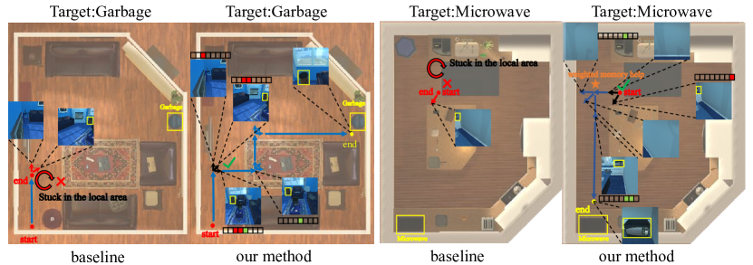
Figure 5. Visualization of the testing process. The target is selected by the yellow box. Some key frames are selected to illustrate the working process of our method.

4.2. Comparisons to the State-of-the-art

To demonstrate the superiority of our method, our method is compared with some recent methods. The results of the comparative experiments are shown in Table 1.

Table 1. Comparisons with the state-of-the-art methods on the AI2-Thor/RoboTHOR datasets

Method	ALL ($\%$)			$L\geqslant 5$ ($\%$)			Episode Time (s)
	SR	SPL	SAE	SR	SPL	SAE
SP(Yang et al., 2018)	62.59/23.73	37.91/15.94	24.55/17.81	52.36/19.47	33.61/14.27	22.67/15.39	0.33/1.37
SAVN(Wortsman et al., 2019)	63.34/25.82	37.16/16.68	20.55/15.69	52.23/20.55	34.94/14.37	23.15/15.79	0.31/1.40
SA(Mayo et al., 2021)	66.51/27.54	38.35/17.37	21.71/16.35	54.53/21.53	34.34/15.79	25.58/16.09	0.31/1.29
ORG(Du et al., 2020a)	67.84/29.87	36.94/18.34	26.18/16.78	58.58/22.43	35.61/17.58	27.34/15.23	0.25/1.30
HOZ(Zhang et al., 2021)	68.49/30.13	37.51/18.84	25.64/17.63	60.94/23.46	36.57/18.50	27.69/18.33	0.30/1.40
VTNet(Du et al., 2020b)	72.37/34.03	45.47/20.31	30.35/19.44	64.56/30.19	44.37/19.43	31.43/20.63	0.34/1.42
DOA(Dang et al., 2022a)	78.84/37.66	44.27/21.46	31.15/20.53	72.38/32.17	45.51/20.73	36.02/21.29	0.37/1.37
OMT(Fukushima et al., 2022)	70.54/33.81	30.43/19.31	26.14/18.16	59.78/29.47	26.31/19.63	24.37/19.14	0.68/1.53
SSCNav(Liang et al., 2021)	76.28/37.06	24.43/13.88	26.58/16.34	68.11/31.24	29.93/14.35	24.97/15.34	1.46/4.96
PONI(Ramakrishnan et al., 2022)	79.64/38.73	35.60/14.26	28.19/17.35	73.28/33.46	36.37/15.34	29.37/18.76	1.83/5.04
DAT(Dang et al., 2022b)	80.95/39.82	46.02/25.34	31.69/22.37	73.86/34.33	46.48/20.47	35.91/23.15	0.32/1.34
Our	82.99/42.07	47.40/27.47	33.04/24.42	77.95/37.26	48.78/22.23	37.69/25.04	0.38/1.35

It can be seen that the performance of our method shows a large advantage. Importantly, our method outperforms current SOTA method (DAT) with the gains of 2.04/2.25, 1.38/2.13, 1.35/2.05 (AI2-Thor/RoboTHOR, $\%$) in SR, SPL and SAE, this result demonstrates the effectiveness and efficiency of our proposed method. Compared with other end-to-end methods, although the semantic map-based methods show greater advantages in SR, these methods spend a lot of time exploring environment and constructing semantic map, which leads to their poor performance on SPL and SAE. And semantic map-based methods take much longer episode time (s), which is unacceptable in practical tasks. Although our method does not show a great advantage in terms of episode time (s), the episode time that the model takes is still acceptable. Moreover, our method obtains the gains of 3.35/3.34 (AI2-Thor/RoboTHOR, $\%$) in SR over the semantic map-based SOTA method PONI, which shows that the semantic map built on the depth image does not show great advantage due to noise interference, and also verifies that our method has good robustness.

4.3. Ablation Experiments

4.3.1. Baseline.

Our baseline is composed of an image feature extractor and target memory. As shown in Figure 2, the resnet18 and the DETR are included in the image feature extractor, and the object features obtained by DETR are assigned learnable weights (Dang et al., 2022a). The construction process of the target memory is detailed in Section 3.3. All the target orientation features in the target memory are averaged to obtain the target orientation embedding feature. The traditional sparse reward is used to train the model.

In order to study the impact of implicit obstacle map (IOM), non-local target memory aggregation (NTWA), and reward mechanism (RM) on the model, a series of ablation experiments are designed to demonstrate the effectiveness of these modules. The results of the ablation experiments on the AI2-Thor are shown in Table 2.

Table 2. Ablation experiment results for IOM, NTWA, and RM

IOM	NTWA	RM	ALL ($\%$)			$L\geqslant 5$ ($\%$)
			SR	SPL	SAE	SR	SPL	SAE
			78.51	46.50	30.09	71.45	46.42	34.07
✓			81.04	46.61	31.58	74.25	46.88	35.43
	✓		80.24	47.49	30.48	73.11	47.78	34.87
		✓	78.72	46.14	28.93	72.05	46.46	33.96
✓	✓		82.23	46.93	31.22	76.97	47.35	35.52
✓		✓	81.87	47.46	32.54	75.83	48.28	35.39
	✓	✓	80.59	47.48	31.20	73.17	47.53	34.88
✓	✓	✓	82.99	47.40	33.04	77.95	48.78	37.69

4.3.2. Implicit obstacle map.

Compared with the baseline, the performances of the IOM-based model are improved by 2.53/2.8, 1.49/
1.36 (ALL/$L\geqslant 5$, $\%$) in SR and SAE, which indicates that IOM does help the model improve performance. However, the improvement of the model in SPL is very small, which shows that the IOM-based model may avoid obstacles with the help of IOM, but the agent does not choose the optimal path to approach the target object. After introducing the RM on the IOM-based model, the SPL of the model is improved by 0.96/1.86 (ALL/$L\geqslant 5$, $\%$), which indicates that the RM increases the efficiency of IOM-based model. Most importantly, after using NTWA to process the target memory, the SR of the IOM-based model has been greatly improved. Compared with the baseline, SR is improved by 3.72/5.52 (ALL/$L\geqslant 5$, $\%$). Since NTWA assigns large weights to the important target orientation features, the cooperation between IOM and important target orientation features greatly improves the performance of the model. The IOM-NTWA-based model also encounters the same problem: compared with the IOM-based model, the performance improvement of SRL is very small, only 0.43/0.93 (ALL/$L\geqslant 5$, $\%$). After adding RM on the basis of IOM and NTWA, the performance of IOM-NTWA-based model has been greatly improved. Compared with the baseline, the IOM-NTWA-RM-based model is improved by 4.48/6.5, 0.9/2.36, 2.95/3.62 (ALL/$L\geqslant 5$, $\%$) in SR, SPL, and SAE, which proves that the introduction of RM makes the cooperation between IOM and NTWA more perfect, and allows our model to outperform existing SOTA methods.

4.3.3. Non-local Target Memory Aggregation.

After introducing the NTWA in the baseline, SR, SPL, and SAE are improved by 1.73/1.66, 0.99/1.36, 0.39/0.8 (ALL/$L\geqslant 5$, $\%$), which shows that the agent can understand important target orientation information through NTWA, and the ability of navigation is improved. And the experimental results of the NTWA-based model, IOM-NTWA-based model, and IOM-NTWA-RM-based model show that the role of NTWA is irreplaceable. It can be seen from Table 2 that RM has very little promotion effect on NTWA, the SR and SAE are only improved by 0.35/0.06, 0.72/0.01 (ALL/$L\geqslant 5$, $\%$), and even SPL shows a negative growth. This shows that RM is more helpful to IOM than to NTWA.

4.3.4. Reward Mechanism.

From the results in Table 2, it can be seen that only using RM does not greatly improve the performance of the model. Compared with the baseline, SR only improves by 0.1. In the absence of IOM and NTWA, the agent cannot understand the reward signal given by RM. Our proposed RM can only further amplify the positive influence of IOM and NTWA in the navigation model and cannot affect the performance of the model alone.

4.4. Importance Analysis of IOM and NTWA

4.4.1. Irreplaceability of IOM and NTWA

In order to demonstrate that the IOM and NTWA are important and irreplaceable, some other schemes are introduced in the baseline and then compared with the IOM-based model and NTWA-based model. Comparison experiments on the AI2-Thor are shown in Table 3 and Table 4.

Table 3. Comparison experiment results for IOM, TPN, and GM

Method	ALL ($\%$)			$L\geqslant 5$ ($\%$)
	SR	SPL	SAE	SR	SPL	SAE
baseline	78.51	46.50	30.09	71.45	46.42	34.07
GM	76.07	43.99	28.34	66.62	42.61	31.62
TPN	79.63	45.02	29.00	72.51	45.74	34.15
IOM	81.04	46.61	31.58	74.25	46.88	35.43

For the IOM, 1) Tentative policy network (TPN) (Du et al., 2020a) is introduced in the baseline for comparative experiments. TPN is to solve the problem that the agent is stuck in the deadlock state, which is similar to the problem that IOM needs to solve. 2) The grid map(GM) (Luo et al., 2022) is used to represent the free space of the agent. GM directly expresses the passable area of the agent to help the agent avoid obstacles. In our work, the size of GM is set to 40*40, and the CNN is used to extract the features of GM. The comparison results of the TPN-based method, the GM-based method, and the IOM-based method are shown in Table 3. It can be seen that the IOM-based method exceeds the TPN-based method and the GM-based method in all aspects of evaluation metrics. By the way, TPN is also a method that focuses on choosing the appropriate action from the experience pool. The pseudo-label actions output by TPN may still not be able to help the agent get out of the deadlock state. The IOM-based method can continuously correct errors according to the implicit obstacle distribution, and then completes obstacle avoidance, the model remains robust even in unseen environments. As can be seen from Table 3, the layout information included in GM is too sparse, making the agent difficult to obtain useful obstacle information, so the performance of the GM-Based model is not as good as that of the IOM-Based model.

For the NTWA, 1) baseline. In the baseline, all the target orientation features in the target memory are averaged, which is also a method to extract features. 2) Target-Aware Multi-Scale Aggregator (TAMSA) (Dang et al., 2022b), TAMSA uses multi-scale one-dimensional convolutions to extract target memory features. The results of the experiment are shown in Table 4.

Table 4. Comparison experiment results for NTWA, baseline, and TAMSA

Method	ALL ($\%$)			$L\geqslant 5$ ($\%$)
	SR	SPL	SAE	SR	SPL	SAE
baseline	78.51	46.50	30.09	71.45	46.42	34.07
TAMSA	79.22	46.48	30.21	72.65	46.53	34.62
NTWA	80.24	47.49	30.48	73.11	47.78	34.87

It can be seen that the performance of the NTWA-based method is better than the baseline and TAMSA-based method, which shows that assigning reasonable weights to the important target orientation features improve the ability of the agent locating the target. By the way, for the initial stage of an episode, in order to ensure that the size of the target memory is fixed, the target memory embedding features extracted by TAMSA include too many “0”, which limits the navigation capabilities of the model. Since attention is used in the NTWA-based method, there is no need to fill the target memory with “0” to fix its size, which ensures the reliability of embedding features.

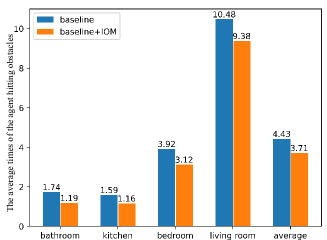
Figure 6. The figure represents the average times of the agent based on the different methods colliding with obstacles.

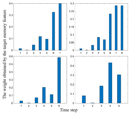
Figure 7. The figure represents the weights assigned by NTWA to different target orientation features.

4.4.2. Does IOM help the agent improve the obstacle avoidance ability?

If the IOM helps the agent to avoid obstacles, there should be two obvious phenomena: the rotation times of the agent are reduced; and the times of the agent colliding with obstacles in the scene are reduced. From Table 3, the SAE of the IOM-based method is 1.49/1.36 (ALL/$L\geqslant 5$, $\%$) higher than the baseline, which shows the frequency of agent’s rotation is reduced. For the 4 test room layouts(AI2-Thor), the average times of the IOM-base agent and baseline-base agent colliding with obstacles are shown in Figure 6. The times of the agent colliding with obstacles in the test scenes are also reduced. In a word, IOM does help the agent improve the ability to avoid obstacles.

4.4.3. How does the NTWA assign weights to target memory?

Taking an episode as an example, the weights assigned by NTWA to the target orientation features are shown in Figure 7. The larger the value of abscissa in the figure, the closer the time interval between the target orientation features and the current state. As can be seen from the figure, NTWA prefers to assign larger weights to the target orientation features that are closer to the current state, which indicates that the features that are closer to the current state are more important.

4.5. Qualitative Analysis

Two typical cases are chosen for visualization in Figure 5. The target of the first case is the “Garbage”. Since the baseline model cannot obtain the obstacle distribution information from the image, the agent is stuck in front of the table, failing in the navigation task. In our method, the implicit obstacle map encodes the obstacle distribution(Red squares indicate impassable directions, green squares indicate passable directions), so the agent quickly finds the passable direction and avoids the table, then navigates to the target object. The target of the second case is “Microwave”. Because the agent in the baseline cannot understand the surrounding obstacle distribution and stops at the initial position. Our method successfully avoids obstacles with the help of the implicit obstacle map. More importantly, since the agent obtains target orientation information by the non-local target memory aggregation, it finds the correct location of the target object when the target disappears in the its view, and completes the navigation task excellently.

5. Conclusion

In this paper, we first proposed an implicit obstacle map module to help the agent avoid obstacles, a non-local target memory aggregation was also designed to obtain target orientation embedding features and help the agent locate the target, and a new reward mechanism was then designed to maximize the potential of the implicit obstacle map and non-local target memory aggregation. A large number of experimental results showed that our model not only guided the agent well to avoid obstacles, but also improved the agent’s navigation efficiency under the cooperation of the implicit obstacle map, non-local target memory aggregation, and new reward mechanism.

- (1)
- Anderson et al. (2018) Peter Anderson, Angel Chang, Devendra Singh Chaplot, Alexey Dosovitskiy, Saurabh Gupta, Vladlen Koltun, Jana Kosecka, Jitendra Malik, Roozbeh Mottaghi, Manolis Savva, et al. 2018. On evaluation of embodied navigation agents. arXiv preprint arXiv:1807.06757 (2018).
- Campari et al. (2020) Tommaso Campari, Paolo Eccher, Luciano Serafini, and Lamberto Ballan. 2020. Exploiting scene-specific features for object goal navigation. In European Conference on Computer Vision. 406–421.
- Carion et al. (2020) Nicolas Carion, Francisco Massa, Gabriel Synnaeve, Nicolas Usunier, Alexander Kirillov, and Sergey Zagoruyko. 2020. End-to-end object detection with transformers. In European Conference on Computer Vision. 213–229.
- Chaplot et al. (2019) Devendra Singh Chaplot, Dhiraj Gandhi, Saurabh Gupta, Abhinav Gupta, and Ruslan Salakhutdinov. 2019. Learning to explore using active neural SLAM. In International Conference on Learning Representations.
- Chaplot et al. (2020) Devendra Singh Chaplot, Dhiraj Prakashchand Gandhi, Abhinav Gupta, and Russ R Salakhutdinov. 2020. Object goal navigation using goal-oriented semantic exploration. Advances in neural information processing systems 33 (2020), 4247–4258.
- Dang et al. (2022a) Ronghao Dang, Zhuofan Shi, Liuyi Wang, Zongtao He, Chengju Liu, and Qijun Chen. 2022a. Unbiased directed object attention graph for object navigation. In Proceedings of the 30th ACM International Conference on Multimedia. 3617–3627.
- Dang et al. (2022b) Ronghao Dang, Liuyi Wang, Zongtao He, Shuai Su, Chengju Liu, and Qijun Chen. 2022b. Search for or Navigate to? Dual Adaptive Thinking for Object Navigation. arXiv preprint arXiv:2208.00553 (2022).
- Deitke et al. (2020) Matt Deitke, Winson Han, Alvaro Herrasti, Aniruddha Kembhavi, Eric Kolve, Roozbeh Mottaghi, Jordi Salvador, Dustin Schwenk, Eli VanderBilt, Matthew Wallingford, et al. 2020. Robothor: An open simulation-to-real embodied ai platform. In Proceedings of the IEEE/CVF Conference on Computer Vision and Pattern Recognition. 3164–3174.
- Du et al. (2020a) H Du, X Yu, and L Zheng. 2020a. Learning Object Relation Graph and Tentative Policy for Visual Navigation. In European Conference on Computer Vision.
- Du et al. (2020b) Heming Du, Xin Yu, and Liang Zheng. 2020b. VTNet: Visual transformer network for object goal navigation. In International Conference on Learning Representations.
- Fang et al. (2019) Kuan Fang, Alexander Toshev, Li Fei-Fei, and Silvio Savarese. 2019. Scene memory transformer for embodied agents in long-horizon tasks. In Proceedings of the IEEE/CVF Conference on Computer Vision and Pattern Recognition. 538–547.
- Fukushima et al. (2022) Rui Fukushima, Kei Ota, Asako Kanezaki, Yoko Sasaki, and Yusuke Yoshiyasu. 2022. Object memory transformer for object goal navigation. In International Conference on Robotics and Automation. 11288–11294.
- Gadre et al. (2022) Samir Yitzhak Gadre, Kiana Ehsani, Shuran Song, and Roozbeh Mottaghi. 2022. Continuous scene representations for embodied AI. In Proceedings of the IEEE/CVF Conference on Computer Vision and Pattern Recognition. 14849–14859.
- He et al. (2017) Kaiming He, Georgia Gkioxari, Piotr Dollar, and Ross Girshick. 2017. Mask r-cnn. In Proceedings of the IEEE International Conference on Computer Vision. 2961–2969.
- He et al. (2016) Kaiming He, Xiangyu Zhang, Shaoqing Ren, and Jian Sun. 2016. Deep residual learning for image recognition. In Proceedings of the IEEE Conference on Computer Vision and Pattern Recognition. 770–778.
- Hochreiter and Schmidhuber (1997) Sepp Hochreiter and Jurgen Schmidhuber. 1997. Long short-term memory. Neural computation 9, 8 (1997), 1735–1780.
- Hu et al. (2021) Xiaobo Hu, Zhihao Wu, Kai Lv, Shuo Wang, and Youfang Lin. 2021. Agent-centric relation graph for object visual navigation. arXiv preprint arXiv:2111.14422 (2021).
- Hu et al. (2019) Xinxin Hu, Kailun Yang, Lei Fei, and Kaiwei Wang. 2019. Acnet: Attention based network to exploit complementary features for RGBD semantic segmentation. In IEEE International Conference on Image Processing. 1440–1444.
- Izadi et al. (2011) Shahram Izadi, David Kim, Otmar Hilliges, David Molyneaux, Richard Newcombe, Pushmeet Kohli, Jamie Shotton, Steve Hodges, Dustin Freeman, Andrew Davison, et al. 2011. Kinectfusion: real-time 3D reconstruction and interaction using a moving depth camera. In Proceedings of the 24th Annual ACM Symposium on User Interface Software and Technology. 559–568.
- Jiang et al. (2018) Jindong Jiang, Lunan Zheng, Fei Luo, and Zhijun Zhang. 2018. Rednet: Residual encoder-decoder network for indoor RGB-D semantic segmentation. arXiv preprint arXiv:1806.01054 (2018).
- Kolve et al. (2017) Eric Kolve, Roozbeh Mottaghi, Winson Han, Eli VanderBilt, Luca Weihs, Alvaro Herrasti, Matt Deitke, Kiana Ehsani, Daniel Gordon, Yuke Zhu, et al. 2017. Ai2-thor: An interactive 3D environment for visual ai. arXiv preprint arXiv:1712.05474 (2017).
- Li et al. (2021) Weijie Li, Xinhang Song, Yubing Bai, Sixian Zhang, and Shuqiang Jiang. 2021. ION: Instance-level object navigation. In Proceedings of the 29th ACM International Conference on Multimedia. 4343–4352.
- Liang et al. (2021) Yiqing Liang, Boyuan Chen, and Shuran Song. 2021. Sscnav: Confidence-aware semantic scene completion for visual semantic navigation. In IEEE International Conference on Robotics and Automation. 13194–13200.
- Luo et al. (2022) Haokuan Luo, Albert Yue, Zhang-Wei Hong, and Pulkit Agrawal. 2022. Stubborn: A strong baseline for indoor object navigation. In IEEE/RSJ International Conference on Intelligent Robots and Systems. 3287–3293.
- Maksymets et al. (2021) Oleksandr Maksymets, Vincent Cartillier, Aaron Gokaslan, Erik Wijmans, Wojciech Galuba, Stefan Lee, and Dhruv Batra. 2021. Thda: Treasure hunt data augmentation for semantic navigation. In Proceedings of the IEEE/CVF International Conference on Computer Vision. 15374–15383.
- Mayo et al. (2021) Bar Mayo, Tamir Hazan, and Ayellet Tal. 2021. Visual navigation with spatial attention. In Proceedings of the IEEE/CVF Conference on Computer Vision and Pattern Recognition. 16898–16907.
- Mnih et al. (2016) Volodymyr Mnih, Adria Puigdomenech Badia, Mehdi Mirza, Alex Graves, Timothy Lillicrap, Tim Harley, David Silver, and Koray Kavukcuoglu. 2016. Asynchronous methods for deep reinforcement learning. In International Conference on Machine Learning. 1928–1937.
- Mnih et al. (2015) Volodymyr Mnih, Koray Kavukcuoglu, David Silver, Andrei A Rusu, Joel Veness, Marc G Bellemare, Alex Graves, Martin Riedmiller, Andreas K Fidjeland, Georg Ostrovski, et al. 2015. Human-level control through deep reinforcement learning. nature 518, 7540 (2015), 529–533.
- Pal et al. (2021) Anwesan Pal, Yiding Qiu, and Henrik Christensen. 2021. Learning hierarchical relationships for object-goal navigation. In Conference on Robot Learning. 517–528.
- Ramakrishnan et al. (2022) Santhosh Kumar Ramakrishnan, Devendra Singh Chaplot, Ziad Al-Halah, Jitendra Malik, and Kristen Grauman. 2022. Poni: Potential functions for objectgoal navigation with interaction-free learning. In Proceedings of the IEEE/CVF Conference on Computer Vision and Pattern Recognition. 18890–18900.
- Savinov et al. (2018) Nikolay Savinov, Alexey Dosovitskiy, and Vladlen Koltun. 2018. Semi-parametric topological memory for navigation. In International Conference on Learning Representations.
- Schulman et al. (2017) John Schulman, Filip Wolski, Prafulla Dhariwal, Alec Radford, and Oleg Klimov. 2017. Proximal policy optimization algorithms. arXiv preprint arXiv:1707.06347 (2017).
- Sethian (1996) James A Sethian. 1996. A fast marching level set method for monotonically advancing fronts. Proceedings of the national academy of sciences 93, 4 (1996), 1591–1595.
- Snavely et al. (2008) Noah Snavely, Steven M Seitz, and Richard Szeliski. 2008. Modeling the world from internet photo collections. International journal of computer vision 80 (2008), 189–210.
- Vaswani et al. (2017) Ashish Vaswani, Noam Shazeer, Niki Parmar, Jakob Uszkoreit, Llion Jones, Aidan N Gomez, Lukasz Kaiser, and Illia Polosukhin. 2017. Attention is all you need. Advances in neural information processing systems 30 (2017).
- Wortsman et al. (2019) Mitchell Wortsman, Kiana Ehsani, Mohammad Rastegari, Ali Farhadi, and Roozbeh Mottaghi. 2019. Learning to learn how to learn: Self-adaptive visual navigation using meta-learning. In Proceedings of the IEEE/CVF Conference on Computer Vision and Pattern Recognition. 6750–6759.
- Wu et al. (2019) Yi Wu, Yuxin Wu, Aviv Tamar, Stuart Russell, Georgia Gkioxari, and Yuandong Tian. 2019. Bayesian relational memory for semantic visual navigation. In Proceedings of the IEEE/CVF International Conference on Computer Vision. 2769–2779.
- Yang et al. (2018) Wei Yang, Xiaolong Wang, Ali Farhadi, Abhinav Gupta, and Roozbeh Mottaghi. 2018. Visual semantic navigation using scene priors. arXiv preprint arXiv:1810.06543 (2018).
- Ye and Yang (2021) Xin Ye and Yezhou Yang. 2021. Hierarchical and partially observable goal-driven policy learning with goals relational graph. In Proceedings of the IEEE/CVF Conference on Computer Vision and Pattern Recognition. 14101–14110.
- Zhang et al. (2022) Sixian Zhang, Weijie Li, Xinhang Song, Yubing Bai, and Shuqiang Jiang. 2022. Generative meta-adversarial network for unseen object navigation. In European Conference on Computer Vision. 301–320.
- Zhang et al. (2021) Sixian Zhang, Xinhang Song, Yubing Bai, Weijie Li, Yakui Chu, and Shuqiang Jiang. 2021. Hierarchical object-to-zone graph for object navigation. In Proceedings of the IEEE/CVF International Conference on Computer Vision. 15130–15140.
- Zhu et al. (2019) Guangxiang Zhu, Zichuan Lin, Guangwen Yang, and Chongjie Zhang. 2019. Episodic reinforcement learning with associative memory. In International Conference on Learning Representations.
- Zhu et al. (2017) Yuke Zhu, Roozbeh Mottaghi, Eric Kolve, Joseph J Lim, Abhinav Gupta, Li Fei-Fei, and Ali Farhadi. 2017. Target-driven visual navigation in indoor scenes using deep reinforcement learning. In IEEE International Conference on Robotics and Automation. 3357–3364.