Tunable quantum criticality in multi-component Rydberg arrays
Abstract
Arrays of Rydberg atoms have appeared as a remarkably rich playground to study quantum phase transitions in one dimension. One of the biggest puzzles that was brought forward in this context are chiral phase transitions out of density waves. Theoretically predicted chiral transition out of period-four phase is still pending experimental verification mainly due to extremely short interval over which this transition is realized in a single-component Rydberg array. In this letter we show that multi-component Rydberg arrays with extra experimentally tunable parameters provide a mechanism to manipulate quantum critical properties without breaking translation symmetry explicitly. We consider an effective blockade model of two component Rydberg atoms. Weak and strong components obey nearest- and next-nearest-neighbor blockades correspondingly. When laser detuning is applied to either of the two components the system is in the period-3 and period-2 phases. But laser detuning applied to both components simultaneously stabilizes the period-4 phase partly bounded by the chiral transition. We show that relative ratio of the Rabi frequencies of the two components tunes the properties of the conformal Ashkin-Teller point and allows to manipulate an extent of the chiral transition. The prospects of multi-component Rydberg arrays in the context of critical fusion is briefly discussed.
pacs:
75.10.Jm,75.10.Pq,75.40.MgIntroduction. Understanding the nature of quantum phase transitions in low-dimensional systems is a central topic of condensed matter physicsGiamarchi (2004); Tsvelik (2003). One of the most debated and long-standing problem in the theory of phase transitions is a chiral melting of the density-wave order that roots back to the study of adsorbed monolayersden Nijs (1988); Schreiner et al. (1994); Abernathy et al. (1994); Selke and Yeomans (1982); Huse and Fisher (1982); Huse et al. (1983); Huse and Fisher (1984). Recent experiments on Rydberg atoms attracts new attention to this problem now in the context of one-dimensional (1D) quantum chainsKeesling et al. (2019); Chepiga and Mila (2019a, b); Maceira et al. (2022); Giudici et al. (2019); Chepiga and Mila (2021); Whitsitt et al. (2018); Samajdar et al. (2018); Rader and Läuchli (2019). The microscopic Hamiltonian of a Rydberg array can be formulated in terms of hard-core bosons:
| (1) |
where is a Rabi frequency and is the van der Waals potential. The competition between the laser detuning that keeps atom in a Rydberg state and strong van der Waals interaction that blocks simultaneous excitation of multiple atoms within a certain radius realizes a sequence of density-wave lobes with integer periodicities Keesling et al. (2019); Rader and Läuchli (2019). These ordered phases are surrounded by the disordered phase with incommensurate short-range order. Incommensurability signals chiral perturbations in a system that have a drastic effect on the nature of quantum phase transitionsHuse and Fisher (1982); Ostlund (1981); Huse and Fisher (1984).
For chiral perturbations do not appear and the transition, if continuous, is in the Ising universality class. For the transition takes place via an incommensurate Luttinger liquid phase (also known as a floating phase)Rader and Läuchli (2019). The transition out of phase is more complicated. Inside the disordered phase chiral perturbations vanish along commensurate lines with wave-vectors . At the point where a commensurate line hits the boundary of the period-3 phase the transition is conformal in the three-state Potts universality class. Away from this point chiral perturbations are relevant and the transition is believed to be in the Huse-Fisher chiral universality classHuse and Fisher (1984); Samajdar et al. (2018); Chepiga and Mila (2019b); Giudici et al. (2019); Maceira et al. (2022). When chiral perturbations are strong a chiral transition is eventually replaced by a floating phaseChepiga and Mila (2019b); Rader and Läuchli (2019); Maceira et al. (2022).
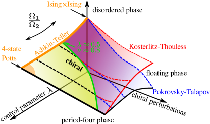
The most intriguing case is . Along the commensurate line the transition is conformalChepiga and Mila (2021) however the underlying Ashkin-Teller critical theory forms a weak universality classKohmoto et al. (1981); Di Francesco et al. (1997). This implies that critical exponents, for instance that describes a divergence of the correlation length, can be continuously tuned by an external parameter Kohmoto et al. (1981). The Ashkin-Teller model interpolates between two decoupled Ising chains at and the symmetric four-state Potts point at (see Fig.1). The exponent as a function of is known exactlyKohmoto et al. (1981); O’Brien et al. (2015):
As sketched in Fig.1 the effect of chiral perturbations that appear in Rydberg arrays away from the commensurate line change the nature of the transitionHuse and Fisher (1984); den Nijs (1988); Nyckees and Mila (2022); Lüscher et al. (2023). When chiral perturbations immediately open a floating phase; when chiral perturbations are also relevant but for a while the transition is direct in the chiral universality classNyckees and Mila (2022); Lüscher et al. (2023); finally, when chiral perturbations are irrelevant and for a certain interval the transition is in the Ashkin-Teller universality class that upon increasing chiral perturbations is followed first by the chiral transition and then by the floating phaseSchulz (1983); Lüscher et al. (2023). In the single-component Rydberg array the conformal Ashkin-Teller point has critical exponent and the second scenario is realizedChepiga and Mila (2021). However, as illustrated in Fig.1, the closer is the Ashkin-Teller point to the shorter is the interval of the chiral transition. As a consequence, the chiral transition in a Rydberg array appears only very close to the conformal pointMaceira et al. (2022) making its experimental investigation extremely difficult.
In this letter we directly address this problem and show how to manipulate quantum critical properties and to enlarge an extent of the chiral transition with two-component bosonic Rydberg array (see below). We show that the ratio between Rabi frequencies of the two components tunes the properties of the Ashkin-Teller multicritical point that in turn controls an appearance and an extent of the chiral transition.
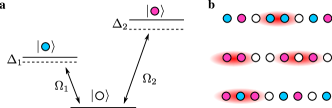
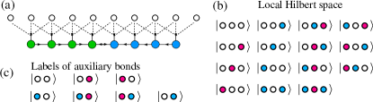
Multi-component Rydberg atoms. Rydberg arrays defined in Eq.1 have two independent parameters while the phase diagram of the chiral Ashkin-Teller modelLüscher et al. (2023) sketched in Fig.1 requires at least three. In recent years there were several proposals aiming to extend the set of control parameters in Rydberg atomsSingh et al. (2022); Sheng et al. (2022); Levi et al. (2015); Lan et al. (2016); Eck and Fendley (2023); Beradze et al. (2023); Fromholz et al. (2022). Among them the multi-speciesSingh et al. (2022); Sheng et al. (2022) and the multi-componentLevi et al. (2015); Lan et al. (2016) Rydberg arrays seems the most promising. In multi-species setup a certain arrangements of Cs and Rb atoms is prepared. Rabi frequency, laser detuning and van der Waals potential can be individually controlled for each individual specimen in addition to the inter-species interaction, so the effective model spans over six-dimensional parameter space. In multi-component Rydberg atoms, only one type of atoms is used but each atom can be excited to one of the two Rydberg levels - components as sketched in Fig.2. The levels can be selected such that (i) first-component interaction is much stronger than the second component one; and (ii) all other interactions including those between different components are negligibly small. This model has five independent parameters: inter-atomic spacing, two Rabi frequencies and and two individually controlled laser detunings and (see Fig.2). Between two set-ups - multi-species and multi-component arrays - the latter has one significant advantage in the context of quantum phase transition and chiral melting: it preserves translation symmetry.
The blockade model. Because of the very fast increase of the van der Waals potential at short distances simultaneous occupation of atoms within certain blockade radius is essentially excluded. It allows us to approximate long-range interactions of two components with two types of Rydberg blockade: nearest-neighbor blockade for the weak and next-nearest-neighbor one for the strong components. This effectively fixes two parameters - relative interaction strength of two species and an interatomic distance. The resulting model is defined by the following microscopic Hamiltonian acting in a constrained Hilbert space:
| (2a) | |||
| (2b) |
Here brings an atom at site from the ground-state to a first or second Rydberg level if or correspondingly. This model has three independent parameters that we define as , , and . We study the model with state-of-the-art DMRG algorithmWhite (1992); Schollwöck (2005); Östlund and Rommer (1995); Schollwöck (2011) with up to sites keeping up to 2500 states and performing up to 8 sweeps (see Supplemental materialsSM for details).
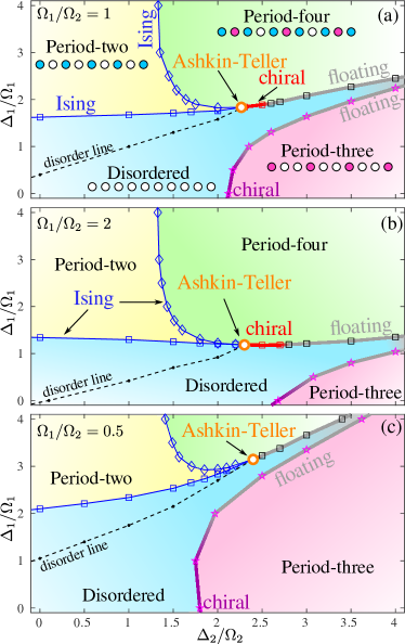
Phase diagram. Our main results are summarized in three phase diagrams in Fig.3. When laser detunings are small the system is in the disordered phase and translation symmetry is not broken. For the system is populated with the strong component that due to next-nearest-neighbor Rydberg blockade leads to a period-three phase separated from the disorder phase by either chiral transition or the floating phaseSM . In the opposite limit the system is in the period-two phase with every other site occupied by a weak component; the transition to the disordered phase is in the Ising universality phaseSM . Upon increasing the detuning the system undergoes the second Ising transitionSM where the translation symmetry is spontaneously broken once again and every other empty site of the period-2 phase is occupied by the strong component resulting in the period-four phase (sketched in Fig.3(a)) with broken symmetry (see Supplemental materialsSM for further details). Upon increasing two Ising lines come closer and eventually merge into a multicritical point in the Ashkin-Teller universality clasDi Francesco et al. (1997). Beyond this point the transition from the disordered to the period-four phases is either direct in the chiral universality class or via the floating phase as shown in Fig.3. This is further suported by incommensurate correlations that weak component develops beyond the disorder lineSM .
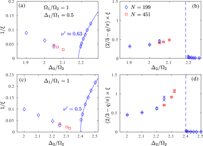
We distinguish three types of transitions - Ashkin-Teller, chiral and floating phase - by looking at the product , where is incommensurate wave-vector approaching its commensurate value with the critical exponent and is a correlation length diverging with the critical exponent . To the best of our knowledge for the Ashkin-Teller criticality the exact value of is not known but according to Huse and Fisher Huse and Fisher (1982, 1984). Then for the Ashkin-Teller point the product is expected to vanish. By contrast, at the chiral transition the equality should hold and takes some finite value. In case of the floating phase, it is separated from the disordered phase by the Kosterlitz-Thouless transitionKosterlitz and Thouless (1973) characterized by the stretch-exponential divergence of correlation length, at the same time the wave-vector remains incommensurate across the transition, therefore diverges.
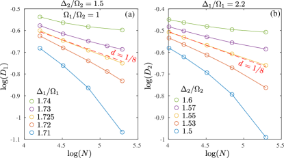
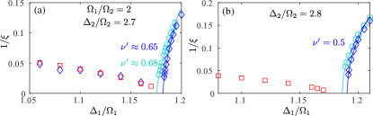
In Fig.4 we show the inverse of the correlation length and the product across different cuts through the transition. For and presented in Fig.4(a),(b) the divergence of the correlation length is symmetric and numerically extracted critical exponent is consistent with the Ashkin-Teller critical theory; the product vanishes. This Ashkin-Teller point belongs to the interval where chiral perturbations results into a chiral transitionNyckees and Mila (2022); Lüscher et al. (2023). Indeed, already at the product shown in Fig.4(c) takes some finite value at the transition. This picture remains valid up to . The location of the transition is extracted by fitting the correlation length in the period-four phaseSM . For presented in Fig.4(d) we see a sign of divergence of signaling the opening of the floating phase.
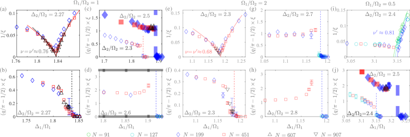
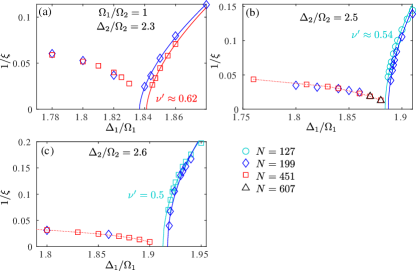
For the larger ratio of Rabi frequencies the location of the Ashkin-Teller point is almost the same but the extracted critical exponent is noticeably smaller (see Fig.4(e),(f)). Beyond this point we detect the chiral transition that extends at least up to as shown in Fig.4(g). In Fig.4(h) for one can clearly see a divergence of upon approaching the floating phase. The larger interval of the chiral transition compare to the previous case with is fully consistent with smaller critical exponent at the Ashkin-Teller point(see Fig.4(e)). In other words, by increasing one can tune the multicritical Ashkin-Teller point towards larger and smaller , that in turns lead to a longer chiral transition as sketched in Fig.1. Note also that the difference between the chiral transition and floating phase is more pronounced for .
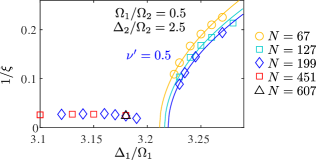
For the multicritical point is very close to the period-three phase and the floating phase surrounding it, as a consequence the correlation length is very large all over the narrow window of the disordered phase. This prevents us from fitting the divergence of the correlation length inside the disordered phase but the product computed locally remains a valid measure: it goes to zero at the Ashkin-Teller point at (see Fig.4(i)-(j)), while for it already shows a signature of divergence suggesting the presence of the floating phase. The latter is further supported by the divergence of the correlation length with the Pokrovsky-Talapov critical exponent (see Supplemental materials SM ). The picture is completed by the observation that along the cut through the Ashkin-Teller point the correlation length diverges with the critical exponent that lies outside of the interval where chiral transition is possible. Of course, neither this interval nor the critical exponents are exact and we cannot exclude a possibility of a short chiral transition between and . But what we observe here is a very important tendency of the Ashkin-Teller critical exponent to increase with decreasing such that the chiral transition shrinks to the point when it eventually disappears.
Discussion. To summarize, our results offer a novel approach to manipulate quantum criticality in Rydberg atoms that, in particular, overcomes the bottleneck associated with the short extent of the chiral transition. In addition, we formulate a protocol to probe the complete phase diagram of the chiral Ashkin-Teller model. Altogether, these provides an opportunity to explore universal and non-universal properties of chiral transitions - a necessary step towards a formal definition of the chiral universality class. We expect our results obtained for the blockade approximation to be qualitatively correct for the model with potential as soon as the selected Rydberg levels and the lattice spacing are such that detuning of weak and strong components alone leads to stable period-two and period-three phases correspondingly. Multi-component Rydberg arrays opens a unique opportunity to explore fusion rules of quantum criticalities directly on a lattice. Here we focused on the simplest case: fusion of two Ising transitions into the Ashkin-Teller point followed by the chiral transition. Playing with different interaction regimes and longer blockades one can realize, for instance, a fusion of chiral transitions. Further generalization to three and more components is conceptually straightforward and introduces a new class of models with multi-component Hilbert space. Multiple individually controllable parameters enables a fine-tuning, for instance, to points with higher symmetries.
I Acknowledgments
I thank Bernhard Lüscher, Samuel Nyckees and Frederic Mila for insightful discussions on the chiral Ashkin-Teller model and to Jiri Minar for inspiring discussion on multi-component Rydberg arrays. This work has been supported by the Delft Technology Fellowship and it was performed in part at Aspen Center for Physics, which is supported by National Science Foundation grant PHY-2210452. Numerical simulations have been performed at the DelftBlue HPC and at the Dutch national e-infrastructure with the support of the SURF Cooperative.
References
- Giamarchi (2004) T. Giamarchi, Quantum physics in one dimension, Internat. Ser. Mono. Phys. (Clarendon Press, Oxford, 2004).
- Tsvelik (2003) A. M. Tsvelik, Quantum Field Theory in Condensed Matter Physics, 2nd ed. (Cambridge University Press, 2003).
- den Nijs (1988) M. den Nijs, Phase Transitions and Critical Phenomena 12, 219 (1988).
- Schreiner et al. (1994) J. Schreiner, K. Jacobi, and W. Selke, Phys. Rev. B 49, 2706 (1994).
- Abernathy et al. (1994) D. L. Abernathy, S. Song, K. I. Blum, R. J. Birgeneau, and S. G. J. Mochrie, Phys. Rev. B 49, 2691 (1994).
- Selke and Yeomans (1982) W. Selke and J. M. Yeomans, Zeitschrift für Physik B Condensed Matter 46, 311 (1982).
- Huse and Fisher (1982) D. A. Huse and M. E. Fisher, Phys. Rev. Lett. 49, 793 (1982).
- Huse et al. (1983) D. A. Huse, A. M. Szpilka, and M. E. Fisher, Physica A: Statistical Mechanics and its Applications 121, 363 (1983).
- Huse and Fisher (1984) D. A. Huse and M. E. Fisher, Phys. Rev. B 29, 239 (1984).
- Keesling et al. (2019) A. Keesling, A. Omran, H. Levine, H. Bernien, H. Pichler, S. Choi, R. Samajdar, S. Schwartz, P. Silvi, S. Sachdev, P. Zoller, M. Endres, M. Greiner, Vuletić, V. , and M. D. Lukin, Nature (London) 568, 207 (2019).
- Chepiga and Mila (2019a) N. Chepiga and F. Mila, SciPost Phys. 6, 33 (2019a).
- Chepiga and Mila (2019b) N. Chepiga and F. Mila, Phys. Rev. Lett. 122, 017205 (2019b).
- Maceira et al. (2022) I. A. Maceira, N. Chepiga, and F. Mila, Phys. Rev. Res. 4, 043102 (2022).
- Giudici et al. (2019) G. Giudici, A. Angelone, G. Magnifico, Z. Zeng, G. Giudice, T. Mendes-Santos, and M. Dalmonte, Phys. Rev. B 99, 094434 (2019).
- Chepiga and Mila (2021) N. Chepiga and F. Mila, Nature Communications 12, 1 (2021).
- Whitsitt et al. (2018) S. Whitsitt, R. Samajdar, and S. Sachdev, Phys. Rev. B 98, 205118 (2018).
- Samajdar et al. (2018) R. Samajdar, S. Choi, H. Pichler, M. D. Lukin, and S. Sachdev, Phys. Rev. A 98, 023614 (2018).
- Rader and Läuchli (2019) M. Rader and A. M. Läuchli, “Floating phases in one-dimensional rydberg ising chains,” (2019), arXiv:1908.02068 [cond-mat.quant-gas] .
- Ostlund (1981) S. Ostlund, Phys. Rev. B 24, 398 (1981).
- Kohmoto et al. (1981) M. Kohmoto, M. den Nijs, and L. P. Kadanoff, Phys. Rev. B 24, 5229 (1981).
- Di Francesco et al. (1997) P. Di Francesco, P. Mathieu, and D. Sénéchal, Conformal Field Theory, Graduate Texts in Contemporary Physics (Springer, New York, 1997).
- O’Brien et al. (2015) A. O’Brien, S. D. Bartlett, A. C. Doherty, and S. T. Flammia, Phys. Rev. E 92, 042163 (2015).
- Nyckees and Mila (2022) S. Nyckees and F. Mila, Physical Review Research 4, 013093 (2022).
- Lüscher et al. (2023) B. Lüscher, F. Mila, and N. Chepiga, arXiv e-prints , arXiv:2308.07144 (2023).
- Schulz (1983) H. J. Schulz, Phys. Rev. B 28, 2746 (1983).
- Singh et al. (2022) K. Singh, S. Anand, A. Pocklington, J. T. Kemp, and H. Bernien, Phys. Rev. X 12, 011040 (2022).
- Sheng et al. (2022) C. Sheng, J. Hou, X. He, K. Wang, R. Guo, J. Zhuang, B. Mamat, P. Xu, M. Liu, J. Wang, and M. Zhan, Phys. Rev. Lett. 128, 083202 (2022).
- Levi et al. (2015) E. Levi, J. Minář, J. P. Garrahan, and I. Lesanovsky, New Journal of Physics 17, 123017 (2015).
- Lan et al. (2016) Z. Lan, W. Li, and I. Lesanovsky, Phys. Rev. A 94, 051603 (2016).
- Eck and Fendley (2023) L. Eck and P. Fendley, Phys. Rev. B 108, 125135 (2023).
- Beradze et al. (2023) B. Beradze, M. Tsitsishvili, E. Tirrito, M. Dalmonte, T. Chanda, and A. Nersesyan, Phys. Rev. B 108, 075146 (2023).
- Fromholz et al. (2022) P. Fromholz, M. Tsitsishvili, M. Votto, M. Dalmonte, A. Nersesyan, and T. Chanda, Phys. Rev. B 106, 155411 (2022).
- White (1992) S. R. White, Phys. Rev. Lett. 69, 2863 (1992).
- Schollwöck (2005) U. Schollwöck, Rev. Mod. Phys. 77, 259 (2005).
- Östlund and Rommer (1995) S. Östlund and S. Rommer, Phys. Rev. Lett. 75, 3537 (1995).
- Schollwöck (2011) U. Schollwöck, Annals of Physics 326, 96 (2011).
- (37) See Supplemental Material, which includes Refs. White (1992); Schollwöck (2005); Östlund and Rommer (1995); Schollwöck (2011); Di Francesco et al. (1997); Ornstein and Zernike (1914); Maceira et al. (2022); Calabrese and Cardy (2009); Chepiga and Mila (2021, 2019a), for details about the algorithm, further details on various phases, additional numerical results supporting Ising transitions, the extraction of the correlation length and the wave-vector, the transition out of period-three phase, the location of the disorder line, and additional results for the transition out of period-four phase.
- Kosterlitz and Thouless (1973) J. M. Kosterlitz and D. J. Thouless, Journal of Physics C: Solid State Physics 6, 1181 (1973).
- Ornstein and Zernike (1914) L. Ornstein and F. Zernike, Koninklijke Nederlandse Akademie van Wetenschappen Proceedings Series B Physical Sciences 17, 793 (1914).
- Calabrese and Cardy (2009) P. Calabrese and J. Cardy, J. Phys. A: Math. Theor. 42, 504005 (2009).
Supplemental matherial to ”Tunable quantum criticality in multi-component Rydberg arrays”
II Details about the algorithm
We perform numerical simulations with DMRG algorithm in the form of variational optimization of the matrix product states (MPS)White (1992); Schollwöck (2005); Östlund and Rommer (1995); Schollwöck (2011). We implement the blockade by applying a strong penalty terms . We choose the penalty to be : this value is sufficiently strong to keep expectation value of any of the three terms listed above below even in the vicinity of the transition, while this value is not too large to cause instabilities and convergence issues. We also benchmarked our algorithm with constrained DMRG with explicitly implemented blockadesChepiga and Mila (2021, 2019a): the two sets of results do not have any noticeable differences. Quite surprisingly the unconstrained DMRG with the penalty terms turns out to be more efficient for numerical simulations of multi-component Rydberg arrays than the constrained version of the algorithm that by construction obeys a block-diagonal structure. In order to implement constrained DMRG for multi-component system, we generalize the implementation of next-nearest-neighbor blockade described in details Ref.Chepiga and Mila (2021). We span local degrees of freedom over three consecutive Rydberg atoms as sketched in Fig.5(a). This increase the local Hilbert space to listed in Fig.5(b), note that out of total states 10 states violating the blockades were excluded. In this construction, every pair of consequtive MPS have share two Rydberg atoms, therefore one can use the state of these atoms as quantum labels that create one-to-one correspondence between auxiliary legs of MPS. Thes seven labels are listed in Fig.5(c).
Contracting the networks block-by-block allows to reduce the memory cost significantly, however an auxiliary bond of tensors having seven different labels leads to a large number of rather small blocks such that an over-head for a block-by-block operation turns out to be higher than the gain from the lower memory cost. In DMRG simulations we reach the convergence of the systems with up to sites keeping up to 2500 states and performing up to 8 sweeps; we generically discard singular values below .
III Additional details on various phases and boundary conditions
In this section we provide further details on various phases and on the used boundary conditions. As explained in the main text, there are four gapped phases: disordered, and period-2, 3 and 4. Fig.6 present local density profiles along a chain with sites at various characteristic points of the phase diagram for . Fig.6(a) shows the density profile at and in the disordered phase. One can clearly see that in the bulk the density of each component is uniform. Note that the microscopic model does not preserve the number of particles in the weak/strong component, so the density of each component changes continuously all over the disordered phase.
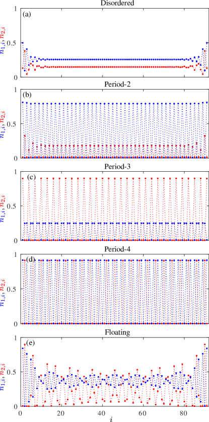
Fig.6(b) presents the density profile at and in the period-2 phase where every other site is occupied by a weak (blue) component. In the thermodynamic limit this phase is two-fold degenerate - weak component can occupy either even or odd sites. In addition one can still detect a small density of the strong (red) component uniformly distributed among sites that are not occupied by a weak component.
Fig.6(c) shows the period-3 phase at and . Every third site is occupied by the strong (red) component, while the remaining sites host a certain density of the weak component uniformly distributed over unoccupied sites. This phase breaks symmetry and in the thermodynamic limit it has three-fold degenerate ground-state.
The density of the period-4 phase taken at and is shown in Fig.6(d). One can see that every second site is occupied by the weak (blue) component, while every other of the remaining sites are occupied by the strong (red) component. This phase spontaneously breaks symmetry and has a four-fold degenerate ground-state in the thermodynamic limit.
Finally, in Fig.6(e) we also present a typical density profile of the floating phase taken in the vicinity of the period-4 phase at and . Note that in the thermodynamic limit the density in this critical phase is uniform and the presence of incommensurability can only be detected via correlation functions. Oscillations in local density that we observe in Fig.6(e) are visible because of explicitly broken translation symmetry due to open boundary conditions.
As one can see in Fig.6(b)-(d), ordered phases favor occupied sites at the edges. This impose boundary conditions to be respected in numerical simulations: for the period-2 phase the total number of sites should satisfy with integer . Period-3 phase requires . In the period-4 phase the edges favor weak-strong-weak cluster over the first and last three sites implying that the chain length should satisfy . As one can easily check used in this paper satisfy all three conditions.
IV Location of the Ising transitions
In order to locate Ising transitions we look at the finite-size scaling of the density oscillations - a local measure of spontaneously broken translation symmetry. In the period-two phase the translation symmetry is broken by the weak component and by two sites, so the relevant operator is defined as that we compute in the middle of the chain. We look at this quantity in the log-scale and associate the transition with the separatrix that separates disordered phase (concave curves) and the symmetry broken phase (convex ones) as shown in Fig.7(a). The slope of the separatrix corresponds to the scaling dimension that is in excellent agreement with the conformal field theory prediction for the Ising transition Di Francesco et al. (1997).
At the transition to the period-four phase the translation is again spontaneously broken: every other site that was not occupied by the weak component in the period-two phase becomes occupied by the strong component in the period-four phase. So the local order parameter can be defined as , where are sites that are not occupied by the weak component. As previously, we associate the transition with the separatrix and its slope is in excellent agreement with the Ising scaling dimension (see Fig.7(b)).
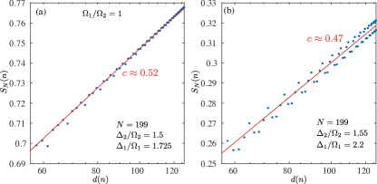
We cross-check the nature of these two transitions by extracting the central charge. The entanglement entropy is extracted from the eigenvalues of the reduced density matrix . We extract central charge numerically from the finite-size scaling of the entanglement entropy in an open chain that on a finite chain with sites scales with the size of the subsystem () asCalabrese and Cardy (2009):
| (3) |
where is the conformal distance and is a non-universal term that includes, in particular, the boundary entanglement entropy. The scaling of the entanglement entropy for the two critical points identified in Fig.7(a),(b) are presented in Fig.7(a) and (b) correspondingly. In both cases the numerically extracted values are in a good agreement with the theory predictions . Small discrepancy is due to a finite resolution of the location of the critical point.
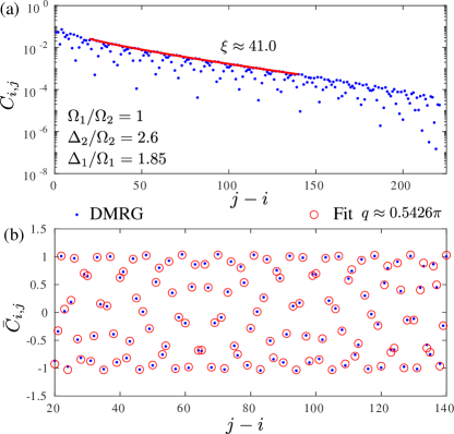
V Extraction of the correlation length and of the wave-vector
In order to extract the correlation length and the wave-vector , we fit the connected correlation function for the strong component to the Ornstein-Zernicke formOrnstein and Zernike (1914):
| (4) |
where the correlation length , the wave vector , and the initial phase are fitting parameters. We extract the correlation length and the wave-vector in two steps. First, we discard the oscillations and fit the main slope of the decay as shown in Fig.9(a) such that the fit can be performed in a semi-log scale . This provides more accurate estimates of the correlation length on a long scale. In fact, there are two very similar strategies to perform this fit: either to fit all the points assuming that oscillations are fast enough to cancel; or to fit only top of the arcs assuming that there are enough arcs for a reliable fit. Here we use the second method and include the point into a fit if it exceeds two points on its left and two points on its right. Let me emphasize here that both methods are equivalent and affect only an amplitude and a centering of a cosine function in the next step.
In the second step we fit the reduced correlation function
| (5) |
with a cosine as shown in Fig.9(b). The agreement between the DMRG data (blue dots) and the fit (red circles) is almost perfect. We estimate error in caused by finite-size effects as , where is a natural step in due to fixed boundary conditions and assuming for infinite correlation length, an additional factor reflect the possibility to adjust at the edges when correlation length is finite.
VI Transition out of period-three phase
In order to locate the boundary of the period-three phase and to identify the nature of the transition we follow a similar procedure as for the boundary of the period-four phase. We look at the product that is expected to take a finite value if transition is chiral and diverge in the case of intermediate floating phase. Here we expect conformal Potts point only in the limit . We also look at the scaling of the correlation length in the period-three phase. In Fig.10 we provide an example of two typical cuts through the transition for : when it is chiral in Huse-Fisher universality class in Fig.10(a),(b); and when it goes through an intermediate floating phase in Fig.10(c),(d). Small increase of in Fig.10(b) indicates its proximity to the Lifshitz point, where the floating phase opens.
Following the same procedure we identified the boundaries of the period-three phase for and . For our results at are consistent with chiral transition, while already at we see a presence of the floating phase. For chiral transition is stable up to and the floating phase is detected at .
VII Disorder line
Chiral perturbations usually manifest itself in incommensurate correlations. The line where real-space correlations switch from commensurate to incommensurate regimes is usually called in the literature the disorder line. In order to locate this line in the disordered phase we look at the connected correlations of the weak component. A few examples of commensurate and incommensurate scalings are shown in Fig.11; we associate the disorder line with the point where incommensurability disappear. Calculations were performed with sites deep inside the disordered phase and with in the vicinity of the multicritical point.
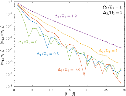
It is not always clear whether the system is commensurate or incommensurate (see, for instance, the data for in Fig.11) and for this reason there is an uncertainty in the location of disorder line. However, our results are consistent with the disorder line hitting the period-four phase at multi-critical point. This agree with expectation that system is commensurate on both sides of the Ising transition. In fact the situation is more subtle here. There are two components and two commensurate Ising transitions. At the transition between the disordered and the period-two phase the weak component breaks translation symmetry and this particular component has to be commensurate in the vicinity of the transition, however the strong component can remain incommensurate across this Ising transition. But at the second Ising transition from period-two to period four phases it is now the strong component that breaks the translation symmetry and thus it has to be commensurate in the vicinity of the transition. It implies that in principle there must be a second disorder line where incommensurability develops in the strong component; this line can be located in the period-two or in the disordered phase and also expected to end at the multicritical Ashkin-Teller point.
VIII Divergence of the correlation length at the transition to the period-four phase
In the main text we distinguished three critical regimes - Ashkin-Teller, chiral and floating phase - by looking at the product . In addition we also extract the critical exponent that controls the divergence of the correlation length upon approaching the boundary of the period-four phase. At the Ashkin-Teller transition and the corresponding results have been presented in Fig.4 (a),(e) and (i) in the main text. For the Pokrovsky-Talapov transition this critical exponent is expected to take the value . For chiral transition the value of this exponent is not known. For and for the two cuts that we identified as a chiral transition based on the extracted critical exponents noticeably exceeds the value of the Pokrovsky-Talapov transition. The results are presented in Fig.12(a),(b). By contrast, at that we identified as a cut through the floating phase the DMRG results are in excellent agreement with .
For and that we associated with chiral transition the critical exponent is about (for smaller system sizes we see ), while for we already see an excellent agreement with the expected square-root divergence. This further supports our conclusion that the Lifshitz point is located in the interval .
Finally, for already at we see that the correlation length diverges with the critical exponent as presented in Fig.14.
For all cuts we see a finite-size effect in the location of the transition. This effect is very common in Rydberg atomsMaceira et al. (2022).