Estimation of equilibration time scales from nested fraction approximations

Abstract

We consider an autocorrelation function of a quantum mechanical system through the lens of the so-called recursive method, by iteratively evaluating Lanczos coefficients, or solving a system of coupled differential equations in the Mori formalism. We first show that both methods are mathematically equivalent, each offering certain practical advantages. We then propose an approximation scheme to evaluate the autocorrelation function, and use it to estimate the equilibration time $\tau$ for the observable in question. With only a handful of Lanczos coefficients as the input, this scheme yields an accurate order of magnitude estimate of $\tau$, matching state-of-the-art numerical approaches. We develop a simple numerical scheme to estimate the precision of our method. We test our approach using several numerical examples exhibiting different relaxation dynamics. Our findings provide a new practical way to quantify the equilibration time of isolated quantum systems, a question which is both crucial and notoriously difficult.

I Introduction

How do many-body quantum systems approach equilibrium? The question to quantify this behavior goes back to the advent of quantum mechanics. Considerable progress has been made in the past decades, with concepts like typicality and the eigenstate thermalization hypothesis having been discovered (and sometimes rediscovered) [1]. However, even the question if an expectation value $\langle O(t)\rangle=\text{Tr}\{O(t)\rho\}$ will reach a certain equilibration value after some time $T$ and never depart from it thereafter (until the Poincaré recurrence time, which is usually parametrically much larger than $T$), for any concrete few-body observable $O$, Hamiltonian $H$, and an initial state $\rho$, can not currently be answered with certainty. An often used concept in this context is the “equilibration on average” [2]. Here, schematically, the frequency of instants in time at which $\langle O(t)\rangle$ significantly deviates from its temporal average, is considered. There are well developed rigorous theorems, asserting this frequency is very small for most practical situations. However, it is very hard (c.f. below) to put a bound on the time interval for which this frequency statement applies. Available rigorous bounds are usually too conservative, exceeding physically observed thermalization time by many orders of magnitude. Furthermore, very odd dynamics that are nevertheless in full accord with the principle of equilibration on average have been demonstrated [3]. While it has been shown that for random Hamiltonians or observables, these equilibration times are typically very short [4, 5, 6, 7, 8, 9, 10, 11], it is easy to construct setups for which they are exceedingly long [4, 5]. There is an extensive literature establishing bounds on equilibration times, both upper bounds [12, 11], as well as lower bounds (often called speed limits) [13]. While these attempts certainly advance the field, many problems limiting their practical applicability remain [14].

In this paper we take a different approach to estimate equilibration time of an isolated quantum system. We focus on the dynamics of autocorrelation functions at infinite temperature, i.e., $C(t)=\text{Tr}\{O(t)O\}$. The latter is in close relation with the dynamics of the expectation values $\langle O(t)\rangle$ for a great variety of initial out of equilibrium states $\rho$ [15, 16]. The time dynamics of $C(t)$ can be expressed using the recursion method or in the Mori formalism. Both approaches parametrize $C(t)$ in terms of a sequence of positive numbers $b_{n}$, called the Lanczos coefficients, which are defined by the pair $O$, $H$. We show that these numbers are the same in both pictures and further elaborate on the relation between these two methods. We then propose an approximation scheme and define $C^{R}(t)$, an approximation to $C(t)$, defined in terms of the first $R$ Lanczos coefficients. Technically, $C^{R}(t)$ is defined by leaving first $R$ coefficients $b_{n}$ intact and declaring $b_{n}=b_{R}$ for $n\geq R$. Strictly speaking $C^{R}(t)$ becomes $C(t)$ only in the limit $R\rightarrow\infty$, but importantly it gives a reasonable approximation for a wide range of times already for modest values of $R$. We develop an indirect quantitative test of accuracy, which can signal that a reasonable approximation of $\tau$ is reached without the need to know the actual $C(t)$. We then use $C^{R}(t)$ to estimate the thermalization time for a number of standard observables and Hamiltonians and find that our method yields reasonable accuracy across the board already with $R<10$. Since computing first $10$ or so Lanczos coefficients for local observables and Hamiltonians with local interactions is usually a straightforward and simple numerical task, our approach readily provides a practical way to estimate the equilibration time for many quantum systems and observables. To summarize, our estimate is not a rigorous bound, but turns out to be very reasonable in all considered examples.

This manuscript is organized as follows. First, in Sec. II, we introduce the recursion method to evaluate the autocorrelation functions. Afterwards, in Sec. III, we give a brief overview of the so-called Mori formalism for correlation functions and show the relation to the Lanczos formulation. We then present a scheme to obtain an approximation for the autocorrelation function within the Mori picture, define suitable equilibration times and establish a convergence criterion based on a pertinent area measure in Sec. IV. Finally, we numerically test our approach for different types of quantum dynamics in Sec. V.

II Recursive method and
Lanczos coefficients

Lanczos coefficients emerge as a part of the so-called recursion method. The object of interest is the autocorrelation functions of the form

$$C(t)=\text{Tr}\{O(t)O\}$$ (1)

with some pertinent observable $O$. Here, $O(t)$ denotes the time dependence in the Heisenberg picture, $O(t)=e^{iHt}\,O\,e^{-iHt}$, induced by corresponding Hamiltonian $H$ ($\hbar$ set to $1$).

In Liouville space, i.e., the Hilbert space of observables, the elements $O$ can be denoted as states $|O)$. The time evolution is then induced by the Liouville superoperator defined as $\mathcal{L}|O)=|[H,O])$. A suitable inner product is given by $(O_{1}|O_{2})=\text{Tr}\{O_{1}^{\dagger}O_{2}\}$, which in turn defines a norm $\|O\|=\sqrt{(O|O)}$. The correlation function $C(t)$ may then be written as $C(t)=(O|e^{i\mathcal{L}t}|O)$.

Now, one may iteratively construct a set of observables $O_{n}$ starting with the “seed” $O_{0}=O$, where $O$ is assumed to be normalized, i.e., $(O_{0}|O_{0})=1$. We set $b_{1}=\|\mathcal{L}O_{0}\|$ and $|O_{1})=\mathcal{L}|O_{0})/b_{1}$. One can now employ the (infinite) iteration scheme

$$|Q_{n}) = \mathcal{L}|O_{n-1})-b_{n-1}|O_{n-2})\ ,$$ (2)

$$b_{n} = \|Q_{n}\|\ ,$$ (3)

$$|O_{n}) = |Q_{n})/b_{n}\ ,$$ (4)

where $\{|O_{n})\}$ constitute the Krylov basis and $b_{n}$ are the Lanczos coefficients, which are real and positive and the crucial constituent in our analysis [17].

Using the Lanczos algorithm, one may cast the time evolution of the components of a vector $\vec{x}$, defined as $x_{n}(t)=i^{-n}(O_{n}|O(t))$, into the form

$$\dot{\vec{x}}=L\,\vec{x}$$ (5)

with the matrix $L$,

$$L=\begin{pmatrix}0&-b_{1}&0&0&\cdots\\ b_{1}&0&-b_{2}&0&\cdots\\ 0&b_{2}&0&-b_{3}&\cdots\\ \vdots&\vdots&\vdots&\vdots&\ddots\end{pmatrix}\,,$$ (6)

which is similar to the standard Schrödinger equation. Then, the first component of $\vec{x}$ is the correlation function of interest, $x_{0}(t)=C(t)$. The initial condition is always given by $x_{n}(0)=\delta_{0n}$.

Note that $L$ is here an anti-Hermitian tridiagonal matrix, but the components $x_{n}$ are all real numbers which is very convenient for the following analysis.

For clarity, the above set of equations may also be written as

$$\dot{x}_{0}(t) = -b_{1}x_{1}(t)\,,$$ (7)

$$\dot{x}_{n}(t) = b_{n}x_{n-1}(t)-b_{n+1}x_{n+1}(t)\,,\quad n\geq 1\,.$$ (8)

That is, the dynamics of the correlation function $C(t)$ may be calculated as occupation amplitude of the “first” site in a one-dimensional non-interacting hopping model without specifying any details of $H$ and $A$.

In the following, we assume that the final Lanczos coefficient $b_{m+1}$ is equal to $0$ (for possibly large $m$). This is always the case for systems with a finite-dimensional Hilbert space. Doing so closes the infinite set of equations in the Lanczos formulation (5), which in turn allows us performing the Laplace transform of the now finite set of equations to arrive at the following finite “continued” fraction expansion. Say, when $m=3$ and $b_{4}=0$ we have explicitly

$$\tilde{x}_{0}(s)=\frac{1}{s+\frac{b_{1}^{2}}{s+\frac{b_{2}^{2}}{s+\frac{b_{3}^{2}}{s}}}}$$ (9)

Here, $\tilde{x}_{0}(s)$ is the Laplace transform of $x_{0}(t)$.

The continued fraction representations of the equations of motion Eq.(8) was given in [18].

In practice the complexity of evaluating $b_{n}$ numerically quickly grows with $n$, such that only a handful first $b_{n}$ are usually available. For a local operator $O$ and a Hamiltonian with local interactions the first coefficients $b_{n}$, up to $n$ of order of the system size, are system size independent. This is an important observation allowing us later to estimate the thermalization time of $C(t)$ in the thermalization limit, when the system is taken to infinity.

III Mori formulation of dynamics

In the previous section we presented the description the correlation function in terms of the recursive method and the Lanczos algorithm. There is an alternative approach of Mori ([19, 20]), with the time evolution specified by a set of functions $C_{n}(t)$ satisfying a coupled series of Volterra equations,

$$\dot{C}_{n}(t)=-\Delta_{n+1}^{2}\int_{0}^{t}C_{n+1}(t-t^{\prime})C_{n}(t^{\prime})dt^{\prime}\ ,$$ (10)

where $C_{0}(t)=x_{0}(t)=C(t)$ is the correlation function itself. Each function satisfies $C_{n}(0)=1$ and $\Delta_{n+1}^{2}C_{n+1}(t)$ acts as a memory kernel for the dynamics of $C_{n}(t)$. The value of constants $\Delta_{n+1}^{2}$ define the value of the memory kernels at time $t=0$.

Both dynamical descriptions are equivalent [21] and as we show momentarily the constants $\Delta_{n}$ are equal to the Lanczos coefficients $b_{n}$.

Within the Mori formulation (10) the condition $b_{m+1}=0$ is equivalent to the condition that the normalized memory kernel $C_{m}(t)$ is a right-continuous Heaviside step function $\Theta(t)$, i.e., $C_{m}(t)$ decays arbitrarily slowly or rather not at all. In this case, Laplace transforming (10) (assuming $m=3$ and $C_{3}(t)=\Theta(t)$) yields

$$\tilde{C}_{0}(s)=\frac{1}{s+\frac{\Delta_{1}^{2}}{s+\frac{\Delta_{2}^{2}}{s+\frac{\Delta_{3}^{2}}{s}}}}\,,$$ (11)

where $\tilde{C}_{0}(s)=\tilde{x}_{0}(s)$ is again the Laplace transform of the autocorrelation function. Continued fraction representations in the context of Mori approach has been formulated in [22].

Comparing the Laplace transforms (9) and (11) readily yields that both dynamical descriptions are equivalent and that $\Delta_{n}=b_{n}$.

The recursive and Mori methods can both be understood from the lens of completely integrable dynamics, see [23].

As a spin-off observation, not related to the following analysis, we note that the time evolution of $C_{n}(t)$ ($n\geq 1$) corresponds to the time evolution of $x_{n}(t)$ but with a time evolution operator obtained by deleting the first $n$ rows and columns of $L$. (Also, the initial conditions are different, $C_{n}(0)=1$ and $x_{n}(0)=0$ for $n\geq 1$.)

IV Approximation of dynamics

IV.1 Memory-kernel approximation

In what follows we assume a thermodynamic limit such that $m$ is either exponentially large or infinite, rendering (9) and (11) infinite continuous fraction expansion.

Our main proposal is that exact dynamics for $C_{0}(t)$ may be reasonably approximated by a suitably “truncated” continuous fraction, not in the sense that the resulting approximate correlation function is very close to $C_{0}(t)$ for all $t$, but that it has approximately the same early $t$ behavior and hence equilibration time (defined below).

Our “truncation” scheme does not assume rendering the sequence of $b_{n}$ finite, but rather we propose to leave the first $R$ coefficients $b_{n}$ intact, while setting all subsequent Lanczos coefficients to be constant $b_{n}=b_{R}$ for all $n\geq R$. Although this may seem to be a radical step from the Lanczos algorithm point of view, it yields a good approximation, as we see below.

From the Mori viewpoint, rendering all $\Delta_{n}=b_{R}$ constant for $n\geq R$ results in a successive application of the same map

$$\tilde{C}_{n-1}(\omega)=\frac{1}{i\omega+b_{R}^{2}\tilde{C}_{n}(\omega)}$$ (12)

Here, instead of $s$ we used $s=a+i\omega$ and note that knowing $\tilde{C}_{n}(s)$ along the imaginary axis is sufficient to perform the inverse Fourier transform and determine $C_{n}(t)$. Successive application of the same transform makes all $\tilde{C}_{n}(\omega)$ for $n\geq R-1$ to be the same, and equal to a fixed point of the map $\tilde{C}_{n}(\omega)=\tilde{S}_{R}(\omega)$ for $n\geq R-1$, where

$$\tilde{S}_{R}(\omega)=-i\frac{\omega}{2b_{R}^{2}}+\frac{1}{b_{R}}\sqrt{1-\left(\frac{\omega}{2b_{R}}\right)^{2}}$$ (13)

for $|\omega|\leq 2b_{R}$, and

$$\tilde{S}_{R}(\omega)=i\left(-\frac{\omega}{2b_{R}^{2}}+\text{sgn}(\omega)\frac{1}{b_{R}}\sqrt{\left(\frac{\omega}{2b_{R}}\right)^{2}-1}\right)$$ (14)

otherwise. Here $\text{sgn}(\omega)$ is the sign function. This result already first appears in [18].

As a result we get the following approximation $\tilde{C}_{R}(\omega)$ to the original exact $\tilde{C}_{0}(\omega)$: with all kernels $\tilde{C}_{n}(\omega)$ being equal to each other for $n\geq R-1$ the continued fraction expansion becomes finite, e.g., for $R=3$,

$$\tilde{C}_{0}^{R=3}(\omega)=\frac{1}{i\omega+\frac{b_{1}^{2}}{i\omega+\frac{b_{2}^{2}}{i\omega+b_{3}^{2}\tilde{S}_{3}(\omega)}}}.$$ (15)

Overall, this approximation is expected to be more accurate as $R$ increases. However, our main point is that in many practical situations it yields a reasonably accurate approximation already for small $R$ ($\leq 10$). In such a case, the Fourier transform of $\tilde{C}_{0}^{R}(\omega)$ can be readily evaluated numerically, giving rise to $C^{R}(t)$. The resulting approximation is therefore determined by a very small number of Lanczos coefficients, $b_{n}$ with $n\leq R$, but, as we see below, gives a good approximation to $C_{0}(t)$ for a wide range of $t$.

IV.2 Equilibration time

We define the equilibration time $\tau$ as the time when the absolute value of $C(t)$ drops below some threshold value $g$ and never exceeds it again, i.e., $\left|C(t)\right|\leq g$ for $t\geq\tau$. Similarly, we denote the equilibration time of $C^{R}$ by $\tau_{a}$ (approximate equilibration time), $\left|C^{R}(t)\right|\leq g$ for $t\geq\tau_{a}$. Our definition differs from other definitions of equilibration time in the literate, e.g., [12]. It is best suited for situations when $C(t)$ decays sufficiently fast. Physically, $\tau$ is characterizing local equilibration. Indeed in most cases $\tau$ is finite in the thermodynamic limit, while global thermalization time, i.e., diffusion time associated with $C(t)\sim t^{-1/2}$ in 1D systems would increase indefinitely with the system size.

Put differently, the definition above is not sensitive to functional behavior of $C(t)$ for large $t$, see the discussion in [24, 25]. Thus even if there is a slow decaying long tail, e.g., $\propto 1/t^{\alpha}$, $\alpha>0$, which is known to be sensitive to $b_{n}$ with very large $n$, the equilibration time $\tau$ may still be sensitive only to a handful of first $b_{n}$.

Our approach is to estimate $\tau$ by evaluating $\tau_{a}$. To characterize the resulting discrepancy we introduce a relative error defined as

$$\varepsilon_{\tau,R}=\left|\frac{\tau_{a}-\tau}{\text{min}(\tau_{a},\tau)}\right|\,.$$ (16)

IV.3 Area estimate and equilibration time

Since the evaluation of $\varepsilon_{\tau,R}$ is not possible without knowledge of the exact $\tau$, below we propose an indirect method to control the precision. Namely, we introduce another measure of precisions and to determine the minimal suitable value of $R$.

To assess the precision, we introduce the “area measure” defined as the area under $C^{R}(t)$,

$$A_{R}=\int_{0}^{\infty}C^{R}(t)dt=\tilde{C}^{R}_{0}(0)\ .$$ (17)

This measure is easily to calculate analytically, yielding

$$A_{R}=\frac{1}{b_{1}}\Pi_{n=1}^{R-1}\left(\frac{b_{n}}{b_{n+1}}\right)^{\left(-1\right)^{n}}\,.$$ (18)

In a similar way we introduce the area under the exact $C(t)$, $A=\tilde{C}_{0}(0)$.

The approximated correlation function $C^{R}(t)$ can only be a good description of $C(t)$ so far the area measures for both are not significantly different from each other. When $R$ increases, $A_{R}$ will converge to $A$ (this statement is intuitive but mathematically subtle, see [26]). We intend to choose $R$ as small as possible, so that $A_{R}$ will not be too different from $A$. As a measure of convergence we can use the relative error

$$\varepsilon_{A,R}=\frac{1}{2}\left(\frac{\left|A_{R}-A_{R+1}\right|}{A_{R}}+\frac{\left|A_{R}-A_{R+2}\right|}{A_{R}}\right)\,,$$ (19)

and choose the smallest $R$, for which $\varepsilon_{A,R}$ falls below some predefined threshold $a$.

We emphasize, that evaluating the area measure (18) is easy and only requires a small number of Lanczos coefficients.

As a consistency check of our proposal we note that for typical quantum systems satisfying the universal operator growth hypothesis of [24] and exhibiting linear growth of Lanczos coefficients $b_{n}=c\,n+d$, the area measure $A_{R}$ converges with the rate $1/R$. We consider an example of a system exhibiting such a behavior below.

There are certainly examples where the area $A$ and hence the approximation (18) diverges, e.g., autocorrelation functions of on-site spin operators in a diffusive $1$-d spin systems, which decay as $\propto 1/\sqrt{t}$. In this case our area-based indirect measure of accuracy is not applicable, although the approach of estimating $\tau$ using $C^{R}(t)$ may still hold.

In the following, our goal is to demonstrate that there is a correlation between the relative area error $\varepsilon_{A,R}$ and the relative equilibration-time error $\varepsilon_{\tau,R}$ such that if $\varepsilon_{A,R}$ is reasonably small, then $\varepsilon_{\tau,R}$ is relatively small as well, which in turn means that $\tau_{a}$ is a reasonable approximation for $\tau$. We show this numerically for several models with different archetypal dynamics.

IV.4 Example: SYK model

First, to illustrate the approach above we consider a standard example of a quantum chaotic system, the SYK model describing $N$ interacting Majorana fermions [27]. This case can be treated semi-analytically. In the large $q$ limit, where $q$ is the number of fermions in the interacting term, the correlation function and the Lanczos coefficients can be described analytically

$$C(t)={1\over\cosh^{\eta}(\alpha t)},\quad b_{n}^{2}=\alpha^{2}n(n+\eta-1),$$ (20)

with some positive $\alpha,\eta$. The same $C(t)$ and $b_{n}$ appear in the context of 2d conformal field theories, with $\alpha$ being related to inverse temperature and $\eta$ to operator’s dimension [28]. The correlation function (20) is decaying exponentially, with the “area measure” (17)

$$A={\Gamma(1/2)\Gamma(\eta/2)\over 2\alpha\Gamma((1+\eta)/2)}$$ (21)

and thermalization time $\tau\approx-\ln g/(\alpha\eta)$.

Now we use our approximation scheme by changing all $b_{n}$ for $n\geq R$ to be $b_{n}=b_{R}$. This behavior is very accurately describing actual Lanczos coefficients in a model of a 1D free scalar field, with a UV cutoff of order $b_{R}$, see [29]. As one may expect, a UV cutoff does not significantly affect the 2-point function until the times inversely proportional to its value. Accordingly, the area measure of the new correlation function (18), which can be evaluated analytically, converges to the true result with the $1/R$ rate,

$$A_{R}=\frac{\sqrt{\pi}\,\Gamma\left(\frac{\eta}{2}\right)\sqrt{\frac{\eta+R-1}{R}}\Gamma\left(\frac{R+1}{2}\right)\Gamma\left(\frac{R+\eta}{2}\right)}{2\Gamma\left(\frac{\eta+1}{2}\right)\Gamma\left(\frac{R}{2}\right)\Gamma\left(\frac{1}{2}(R+\eta+1)\right)}=$$

$$A\left(1-\frac{1}{2R}+\frac{2\eta-1}{8R^{2}}+\dots\right).$$ (22)

This confirms that taking $R\approx 10$ would provide a reasonably good accuracy for the estimation of the area measure. Similarly, $\tau_{a}$ will give a reasonable approximation to $\tau$, as follows from the numerical plot of $C^{R}(t)$ in Fig. 1.

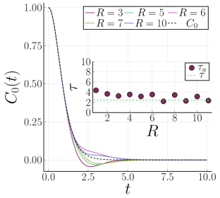
Figure 1: Actual and approximated correlation functions for different values of $R$ for the SYK model with $\eta=2$. Inset shows equilibration times of approximated correlation functions for different values of $R$ with equilibration-time threshold $g=0.03$.

V Numerics

V.1 Tilted-field Ising model

In the following, we test our approach numerically for several typical quantum models. We begin with the tilted-field Ising model, with the Hamiltonian

$$H=H_{0}+B_{x}\sum_{l}\sigma_{x}^{l}\ ,$$ (23)

$$H_{0}=\sum_{l}J\sigma_{x}^{l}\sigma_{x}^{l+1}+B_{z}\sigma_{z}^{l}\ ,$$ (24)

where $\sigma_{x,z}$ are the respective spin components, $J$ is the spin coupling constant, and $B_{x,z}$ are the components of the applied magnetic field. We set $J=1.0$, $B_{z}=-1.05$ and use $B_{x}$ as tunable parameter. For $B_{x}=0$ the magnetic field is not tilted and the model is integrable, whereas for $B_{x}\neq 0$ the model becomes non-integrable. As observable of interest, we consider a fast mode [30]

$$O\propto\sum_{l}\text{cos}(\pi l)h_{l}\,,$$ (25)

with $h_{l}$ being the local energy, i.e., $H=\sum_{l}h_{l}$,

$$h_{l}=J\sigma_{l}^{x}\sigma_{l+1}^{x}+\frac{B_{x}}{2}(\sigma_{l}^{x}+\sigma_{l+1}^{x})+\frac{B_{z}}{2}(\sigma_{l}^{z}+\sigma_{l+1}^{z})\ .$$ (26)

For the calculation, we choose a system with $L=24$ spins and periodic boundary conditions. The dynamics of this observable is the case of a rather fast decaying correlation function, for a further discussion see [31]. The finite length $L$ is only relevant for the numerical calculation of the actual correlation function.

Corresponding Lanczos coefficients are depicted in Fig. 2. These coefficients are system size-independent. Their values are obtained by increasing the length $L$ to be large enough such that finite size effects vanish. (For this model the first $L/2$ Lanczos coefficients correspond to infinite-system values.)

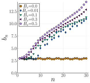
Figure 2: Numerically calculated Lanczos coefficients for the tilted-field Ising model.

V.2 Spin-$1/2$ coupled to an Ising spin bath

Next, we consider a model of a single spin-$1/2$ coupled to a bath, which consists of an Ising spin model with an applied magnetic field. The corresponding Hamiltonian reads

$$H=H_{S}+\lambda H_{I}+H_{B}$$ (27)

with

$$H_{S}=\omega\sigma_{z}^{S}\ ,$$ (28)

$$H_{I}=\sigma_{x}^{S}\sigma_{x}^{0}\ ,$$ (29)

$$H_{B}=\sum_{l}J\sigma_{z}^{l}\sigma_{z}^{l+1}+B_{x}\sigma_{x}^{l}+B_{z}\sigma_{z}^{l}\ .$$ (30)

The parameters are chosen to be

$$\omega=1,\,J=1,\,B_{x}=1,\,B_{z}=0.5\,.$$ (31)

The length of the bath is $L=20$ and we use periodic boundary conditions. Finite $L$ effects are only important for the exact $C(t)$, all evaluated $b_{n}$ are universal. Here $H_{S}$ is the Hamiltonian of the single spin, $H_{B}$ is the bath Hamiltonian, and $H_{I}$ introduces a coupling of the single spin to the first spin of the bath via the corresponding $x$ components. We investigate different scenarios for this model by varying the coupling strength $\lambda$. As observables of interest for the correlation function, we analyze here the $z$-component of the single spin, $O=\sigma_{z}^{S}$, and the respective $x$-component, $O=\sigma_{x}^{S}$.

The Lanczos coefficients are shown in Figs. 3 and 4.

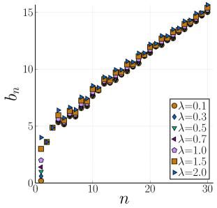
Figure 3: Numerically calculated Lanczos coefficients for $\sigma_{z}^{S}$ in the model of a spin-1/2 coupled to a bath.

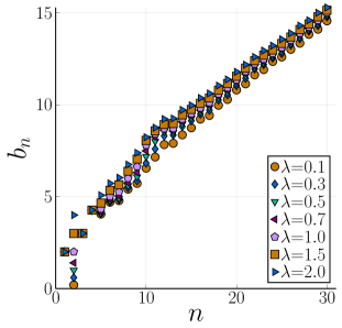
Figure 4: Numerically calculated Lanczos coefficients for $\sigma_{x}^{S}$ the model of a spin-1/2 coupled to a bath.

Note that for both observables all Lanczos coefficients, except for the first one, are very similar. For the observable $\sigma_{z}^{S}$, the first Lanczos coefficient $b_{1}$ is much smaller compared to the others $b_{n}$’s. It decreases for smaller interaction strength $\lambda$. For the observable $\sigma_{x}^{S}$, similar behavior is exhibited by the second Lanczos coefficient $b_{2}$. This feature has an immediate consequence for the value of $A_{R}$. For small coupling strengths $\lambda$, the observable $\sigma_{z}^{S}$ exhibits a slow exponential decay and $\sigma_{x}^{S}$ exhibits a slow, exponentially damped oscillation [32], see Fig. 10. Numerically calculated exact correlation functions for two sets of parameters are shown further below in Figs. 10,11. The curves are obtained using a numerical approach based on quantum typicality [32].

V.3 Numerical equilibration times

We now study how the area estimation criterion can be used to determine the relevant $R$ to achieve a reasonable approximation of $\tau$. In figures 5 and (6) we show the relaxation-time error $\varepsilon_{\tau,R}$ versus the area error $\varepsilon_{A,R}$, for the area-error thresholds $a=0.25$ and $a=0.1$. In both cases, we choose $g=0.03$ as threshold value to define equilibration times $\tau$, $\tau_{a}$ from the numerically calculated curves [32]. While there is no functional dependence visible between $\varepsilon_{A,R}$ and $\varepsilon_{\tau,R}$, one may conclude that, for all cases shown, whenever the area error is below a reasonably small threshold, this assures that $\varepsilon_{\tau,R}$ is also sufficiently small, allowing to estimate $\tau$ from $\tau_{a}$, at lest within an order of magnitude. (A factor $12$ for $a=0.25$ and factor $5$ for $a=0.1$.) Note that points corresponding to, e.g., the largest $R$ do not systematically correspond to smallest $\varepsilon_{\tau,R}$ or $\varepsilon_{A,R}$. Therefore, the area estimation appears to be a useful and easily accessible tool to determine a minimal $R$ for a satisfactory approximation of the correlation function in terms of a finite fraction (11).

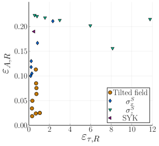
Figure 5: Relative area error $\varepsilon_{A,R}$ (with threshold $a=0.25$) versus relaxation time error $\varepsilon_{\tau,R}$ (with threshold $g=0.03$) for all models considered. All $R$ lie between $1$ and $4$.

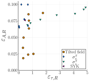
Figure 6: Relative area error $\varepsilon_{A,R}$ (with threshold $a=0.1$) versus relaxation time error $\varepsilon_{\tau,R}$ (with threshold $g=0.03$) for all models considered. All $R$ lie between $1$ and $8$.

Figures 7 and 8 show exact versus approximated relaxation times for all models considered, again for the $R$ determined by the area threshold $a=0.25$ and $a=0.1$. As already visible in Figs. 5 and 6, one finds that approximated and exact relaxation times do not differ substantially from each other. Figures 7 and 8 also show that our models cover a quite large range of equilibration time scales, from fast decay for the tilted field model to slow (exponential) relaxation and oscillation for the spin coupled to a bath model [32]. To further demonstrate the strength of our approach, we compare our approximation of the equilibration time with an estimate of an upper bound of the equilibration time derived in [12], which is depicted in Fig. 9. In [12], this bound $p$ is specified to be proportional to $1/\sqrt{\partial^{2}C_{0}(t=0)/\partial t^{2}}$, which in the Lanczos or Mori formulation amounts to $\propto 1/b_{1}$. (For simplicity, we assume the proportionality constant to be $1$.) We also note that a somewhat similar approach to describe the autocorrelation function with help of the first few coefficients $b_{n}$ with the emphasis on $b_{1}$ was recently undertaken in [33].

Although there are limitations to this comparison, partly because in [12] a rather different definition of equilibration time is employed, one may observe that our estimated equilibration times are systematically much closer to the solid line, which represents the case when actual equilibration time and the approximate one coincide. For the spin coupled to a bath model, the approximation from [12] yields a constant for the $\sigma_{x}^{S}$ component and a square root dependence in the double logarithmic plot for the $\sigma_{z}^{S}$ component, for the small-coupling/large equilibration-time cases. Note that the slow oscillation for the $\sigma_{x}^{S}$ case [32] is basically excluded in [12], because the frequency distribution is not unimodal.

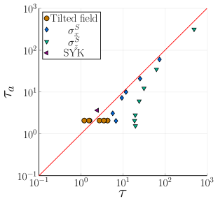
Figure 7: Correct equilibration time $\tau$ versus approximated equilibration time $\tau_{a}$, with $R$ from area threshold $a=0.25$ and equilibration-time threshold $g=0.03$, for all models considered. All $R$ lie between $1$ and $4$.

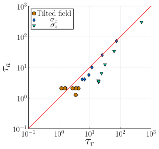
Figure 8: Correct equilibration time $\tau$ versus approximated equilibration time $\tau_{a}$, with $R$ from area threshold $a=0.1$ and equilibration-time threshold $g=0.03$, for all models considered. All $R$ lie between $1$ and $8$.

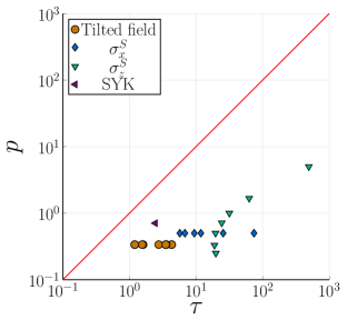
Figure 9: Correct equilibration time $\tau$ versus bound $p$ from [12], with equilibration-time threshold $g=0.03$, for all models considered.

Beyond a mere estimation of equilibration time, we propose that the “terminated” continued fraction (15) may give a reasonable approximation for the actual correlation function itself. To analyze this feature, we show in Figs. 10,11 approximated correlation functions for different values of $R$ for examples that represent cases where our estimation for the equilibration time works best and worst, i.e., $\sigma_{x}^{S}$ for $\lambda=0.5$ (best) and $\sigma_{z}^{S}$ for $\lambda=1.0$ (worst) for the model of a spin-1/2 coupled to a bath. (The examples are chosen according to the smallest and largest relaxation time error $\varepsilon_{\tau,R}$ for area error threshold $a=0.1$ and equilibration-time threshold $g=0.03$.) One finds a very good agreement even for small values of $R$ for the good case, and there is no severe qualitative difference in the behavior in the worst case. For both cases one may deduce that the disagreement becomes smaller for growing $R$ and that there is a convergence for large $R$, although this behavior is not robust for small $R$.

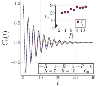
Figure 10: Actual and approximated correlation functions for different values of $R$ for $\sigma_{x}^{S}$, $\lambda=0.5$ in the model of a spin-1/2 coupled to a bath. Inset shows equilibration times of approximated correlation functions for different values of $R$ with equilibration-time threshold $g=0.03$.

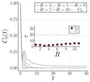
Figure 11: Actual and approximated correlation functions for different values of $R$ for $\sigma_{z}^{S}$, $\lambda=1.0$ in the model of a spin-1/2 coupled to a bath. Inset shows equilibration times of approximated correlation functions for different values of $R$ with equilibration-time threshold $g=0.03$.

VI Conclusion

We have demonstrated that descriptions of the autocorrelation dynamics in the recursive (Lanczos algorithm) and Mori formulations are equivalent and, with help of Laplace transforms, can be recast in terms of a continued fraction expansion. Using this technique we introduced an approximation $C^{R}(t)$ to the autocorrelation function $C(t)$ that is fully determined by a small number of the first $R$ Lanczos coefficients and therefore easy to evaluate numerically in most situations. We have compared suitably defined equilibration times for an actual exact correlation function and the approximation, and found that the latter gives a reasonable estimation for the former. In order to control the precision of our approximation, we introduced an indirect “area measure” which evaluates the area under $C(t)$. This measure is very simple to evaluate and should be considered beforehand to determine the minimal necessary number $R$ of Lanczos coefficient, to achieve the desired level of accuracy. We have numerically validated this approach by comparing how the quality of equilibration time estimation is correlated with the precision in estimating the area measure. We numerically considered several archetypal quantum models that exhibit a variety of different relaxation behavior and a broad range of equilibration time scales.

We envision our approximation scheme for $C(t)$ in terms of $C^{R}(t)$ to be useful for various applications beyond an equilibration time estimation.

References

- Gogolin and Eisert [2016] C. Gogolin and J. Eisert, Equilibration, thermalisation, and the emergence of statistical mechanics in closed quantum systems, Rep. Prog. Phys. 79, 056001 (2016).
- Reimann [2008] P. Reimann, Foundation of statistical mechanics under experimentally realistic conditions, Phys. Rev. Lett. 101, 190403 (2008).
- Knipschild and Gemmer [2020] L. Knipschild and J. Gemmer, Modern concepts of quantum equilibration do not rule out strange relaxation dynamics, Phys. Rev. E 101, 062205 (2020).
- Goldstein et al. [2013] S. Goldstein, T. Hara, and H. Tasaki, Time scales in the approach to equilibrium of macroscopic quantum systems, Phys. Rev. Lett. 111, 140401 (2013).
- Malabarba et al. [2014] A. S. L. Malabarba, L. P. García-Pintos, N. Linden, T. C. Farrelly, and A. J. Short, Quantum systems equilibrate rapidly for most observables, Phys. Rev. E 90, 012121 (2014).
- Reimann [2016] P. Reimann, Typical fast thermalization processes in closed many-body systems, Nat. Commun. 7, 10821 (2016).
- Vinayak and Žnidarič [2012] Vinayak and M. Žnidarič, Subsystem dynamics under random hamiltonian evolution, J. Phys. A: Math. Theor. 45, 125204 (2012).
- Brandão et al. [2012] F. G. S. L. Brandão, P. Ćwikliński, M. Horodecki, P. Horodecki, J. K. Korbicz, and M. Mozrzymas, Convergence to equilibrium under a random Hamiltonian, Phys. Rev. E 86, 031101 (2012).
- Masanes et al. [2013] L. Masanes, A. J. Roncaglia, and A. Acín, Complexity of energy eigenstates as a mechanism for equilibration, Phys. Rev. E 87, 032137 (2013).
- Goldstein et al. [2015] S. Goldstein, T. Hara, and H. Tasaki, Extremely quick thermalization in a macroscopic quantum system for a typical nonequilibrium subspace, N. J. Phys. 17, 045002 (2015).
- Alhambra et al. [2020] A. M. Alhambra, J. Riddell, and L. P. García-Pintos, Time evolution of correlation functions in quantum many-body systems, Phys. Rev. Lett. 124, 110605 (2020).
- García-Pintos et al. [2017] L. P. García-Pintos, N. Linden, A. S. L. Malabarba, A. J. Short, and A. Winter, Equilibration time scales of physically relevant observables, Phys. Rev. X 7, 031027 (2017).
- Hamazaki [2022] R. Hamazaki, Speed limits for macroscopic transitions, PRX Quantum 3, 020319 (2022).
- Heveling et al. [2020] R. Heveling, L. Knipschild, and J. Gemmer, Comment on “Equilibration time scales of physically relevant observables”, Phys. Rev. X 10, 028001 (2020).
- Richter et al. [2019a] J. Richter, J. Gemmer, and R. Steinigeweg, Impact of eigenstate thermalization on the route to equilibrium, Phys. Rev. E 99, 050104 (2019a).
- Richter et al. [2019b] J. Richter, M. H. Lamann, C. Bartsch, R. Steinigeweg, and J. Gemmer, Relaxation of dynamically prepared out-of-equilibrium initial states within and beyond linear response theory, Phys. Rev. E 100, 032124 (2019b).
- Cyrot-Lackmann [1967] F. Cyrot-Lackmann, On the electronic structure of liquid transitional metals, Advances in Physics 16, 393 (1967).
- Haydock [1980] R. Haydock, The recursive solution of the schrödinger equation, Computer Physics Communications 20, 11 (1980).
- Mori [1965a] H. Mori, Transport, collective motion, and Brownian motion, Prog. Theor. Phys. 33, 423 (1965a).
- Joslin and Gray [1986] C. Joslin and C. Gray, Calculation of transport coefficients using a modified Mori formalism, Mol. Phys. 58, 789 (1986).
- Moro and Freed [1981] G. Moro and J. H. Freed, Classical time-correlation functions and the Lanczos algorithm, Journal of Chemical Physics 75, 3157 (1981).
- Mori [1965b] H. Mori, A continued-fraction representation of the time-correlation functions, Progress of Theoretical Physics 34, 399 (1965b).
- Dymarsky and Gorsky [2020] A. Dymarsky and A. Gorsky, Quantum chaos as delocalization in krylov space, Physical Review B 102, 10.1103/physrevb.102.085137 (2020).
- Parker et al. [2019] D. E. Parker, X. Cao, A. Avdoshkin, T. Scaffidi, and E. Altman, A universal operator growth hypothesis, Phys. Rev. X 9, 041017 (2019).
- Viswanath and Müller [2008] V. S. Viswanath and G. Müller, The Recursion Method: Application to Many-body Dynamics (Springer, New York, 2008).
- Viswanath and Müller [1990] V. S. Viswanath and G. Müller, Recursion method in quantum spin dynamics: The art of terminating a continued fraction, Journal of Applied Physics 67, 5486 (1990).
- Maldacena and Stanford [2016] J. Maldacena and D. Stanford, Remarks on the Sachdev-Ye-Kitaev model, Phys. Rev. D 94, 106002 (2016), arXiv:1604.07818 [hep-th] .
- Dymarsky and Smolkin [2021] A. Dymarsky and M. Smolkin, Krylov complexity in conformal field theory, Phys. Rev. D 104, L081702 (2021), arXiv:2104.09514 [hep-th] .
- Avdoshkin et al. [2022] A. Avdoshkin, A. Dymarsky, and M. Smolkin, Krylov complexity in quantum field theory, and beyond, (2022), arXiv:2212.14429 [hep-th] .
- Wang et al. [2022] J. Wang, M. H. Lamann, J. Richter, R. Steinigeweg, A. Dymarsky, and J. Gemmer, Eigenstate thermalization hypothesis and its deviations from random-matrix theory beyond the thermalization time, Phys. Rev. Lett. 128, 180601 (2022).
- Heveling et al. [2022] R. Heveling, J. Wang, and J. Gemmer, Numerically probing the universal operator growth hypothesis, Phys. Rev. E 106, 014152 (2022).
- [32] The numerical calculation of the correct autocorrelation function is done by the use dynamical quantum typicality, see, e.g. [34].
- Zhang and Zhai [2023] R. Zhang and H. Zhai, Universal hypothesis of autocorrelation function from krylov complexity (2023), arXiv:2305.02356 [cond-mat.stat-mech] .
- Heitmann et al. [2020] T. Heitmann, J. Richter, D. Schubert, and R. Steinigeweg, Selected applications of typicality to real-time dynamics of quantum many-body systems, Z. Naturforsch. A 75, 421 (2020).