TrafficMCTS: A Closed-Loop Traffic Flow Generation Framework with Group-Based Monte Carlo Tree Search

Abstract

Digital twins for intelligent transportation systems are currently attracting great interests, in which generating realistic, diverse, and human-like traffic flow in simulations is a formidable challenge. Current approaches often hinge on predefined driver models, objective optimization, or reliance on pre-recorded driving datasets, imposing limitations on their scalability, versatility, and adaptability. In this paper, we introduce TrafficMCTS, an innovative framework that harnesses the synergy of group-based Monte Carlo tree search (MCTS) and Social Value Orientation (SVO) to engender a multifaceted traffic flow replete with varying driving styles and cooperative tendencies. Anchored by a closed-loop architecture, our framework enables vehicles to dynamically adapt to their environment in real time, and ensure feasible collision-free trajectories. Through comprehensive comparisons with state-of-the-art methods, we illuminate the advantages of our approach in terms of computational efficiency, planning success rate, intent completion time, and diversity metrics. Besides, we simulate highway and roundabout scenarios to illustrate the effectiveness of the proposed framework and highlight its ability to induce diverse social behaviors within the traffic flow. Finally, we validate the scalability of TrafficMCTS by showcasing its prowess in simultaneously mass vehicles within a sprawling road network, cultivating a landscape of traffic flow that mirrors the intricacies of human behavior.

I Introduction

Rapid advances in intelligent transport systems and autonomous driving technology have ushered in a revolutionary era in urban transport. Amidst this transformative surge, a key challenge emerges: understanding the complex dynamics of traffic flows. This understanding is crucial for enhancing transportation efficiency, safety, and adaptability. However, obtaining natural driving data from real-world situations is both expensive and time-consuming, often falling short [1, 2, 3]. Real-world traffic encompasses diverse scenarios, making it a formidable obstacle. In light of these challenges, a compelling alternative emerges the concept of generating diverse and human-like traffic patterns within carefully crafted virtual environments. Simulations offer the advantage of providing rich and controllable traffic data that serve multiple purposes [4, 5]. By circumventing the constraints of real-world data collection, simulations promise a dynamic and efficient way of understanding traffic dynamics, fine-tuning strategies, and pushing the boundaries of innovation.

Delving deeper into the studies of traffic simulations, their effectiveness hinges on their ability to replicate the interactive and diverse nature of real-world vehicular environments [6]. The main goal is to achieve a smooth and logical interaction between the ego car and its surroundings vehicles, while also imitating the subtle behaviors of human drivers. However, translating the intricate rhythms of real-world traffic into the realm of simulation presents a considerable challenge [7, 8]. This challenge involves multiple dimensions, including the intricate interplay of road layouts and vehicle dynamics, as well as the subtleties of driver preferences and social interactions. The complexity intensifies when coordinating numerous vehicles while maintaining a balance between consistency and diversity, emphasizing the high demands on traffic flow generation algorithms. In this context, it’s crucial to develop accurate and efficient algorithms to ensure that simulated traffic scenarios authentically capture the intricate dynamics of real-world driving.

Existing open-source traffic simulation tools like SUMO [5] and CARLA [9] have proven useful in generating traffic flows, but they do exhibit certain limitations. These tools rely on simplistic driving models with deterministic parameters, which fail to capture the complexity and variability of human driving behaviors. Consequently, the simulated traffic flows tend to display homogeneous driving behaviors, lacking the necessary nuance. Furthermore, these tools are not adequately refined to handle vehicle lateral dynamics [10]. To solve this problem, multi-vehicle trajectory planning gets much attention in these years, which often optimizes specific objective functions, such as minimizing travel time or maximizing safety for multiple vehicles [11, 12, 13]. However, the existing multi-vehicle trajectory planning methods struggle to handle a large number of vehicles in more complex traffic scenarios, which limits these methods to scale up to large-scale traffic flow generation because of overloaded computing resources and time, making them impractical for real-time traffic simulation. Recent studies, such as InterSim [14], have relied heavily on pre-recorded trajectory datasets, hampering their potential to generate dynamic traffic flow over long periods due to the limited duration of the trajectories in the datasets.

To address these limitations, we propose a novel framework for generating diverse traffic flow with group-based Monte Carlo tree search (MCTS), called TrafficMCTS. Our framework can generate realistic, diverse, and human-like traffic flow within various road conditions under large road networks. Our framework can also efficiently generate traffic flows containing a large number of vehicles. The main contributions of this paper are as follows:

• We propose a novel approach called group-based MCTS, which makes decisions in groups formed based on the possibility of interaction between vehicles. This approach can avoid the exponential increase in exploration difficulty in the MCTS and greatly improve computational efficiency. In comparison to other methods, our approach significantly reduces search time while also maintaining a higher planning success rate and shorter intent completion time.

• We incorporate Social Value Orientation (SVO) to adapt the cooperative tendency of each vehicle to different values, leading to different driving styles within the same scenario. This approach allows us to introduce diversity into the traffic flow at the social interaction level while maintaining interpretability and controllability.

• We present a closed-loop architecture for traffic flow generation that allows vehicles to react to the dynamic environment in real-time while providing collision-free and constraint-satisfying trajectories. Unlike SUMO, our approach takes into account vehicle kinematics and offers flexible right-of-way priorities to vehicles, resulting in more realistic traffic flows. Our architecture is capable of handling up to 80 vehicles simultaneously planning on a road network while maintaining an overall simulation acceleration ratio of over 110%.

II Related Work

This section presents a review of the relevant literature on traffic flow generation. We first introduce some mainstream traffic simulators and then summarize the research work on decision-making and planning for vehicles.

II-A Traffic Simulator

Traffic simulators can provide an effective means of studying traffic phenomena and facilitating the development of autonomous driving technologies. Over the years, some traffic simulators have gained widespread attention and have their characteristics.

II-A1 Simulation for Traffic Management

Traffic simulations have been developing for decades. Typically, PTV Vissim is a commercial microscopic traffic simulation system for modeling highway and urban traffic [15], which can be used to study private and public transport, especially pedestrian traffic. SUMO is an open-source traffic simulator including the simulation itself as well as network import and demand modeling [5], which provides high-performance simulation from a single intersection to an entire city, along with a “remote control” interface. These simulators for traffic management can improve traffic efficiency by exploring adjustments to traffic strategies, such as optimizing signal timing schemes. However, the depictions of fine-grained vehicle motion processes were too simplistic and lacked authenticity.

II-A2 Simulation for Vehicle Dynamics

CarSim provided high-fidelity vehicle dynamics models for virtual testing, simulating braking, handling, ride, stability, and acceleration [16]. TNO’s PreScan and ITS Modeller could form a suite of tools for the design and evaluation of connected vehicle systems [17], where PreScan worked with dedicated vehicle dynamics packages for hardware-in-the-loop simulation and the ITS Modeller was a microscopic traffic simulator where each group of vehicles had its driver behavior, both on a tactical and strategic level. PreScan has been used by over a hundred OEMs and Tier 1 suppliers worldwide for over twenty years. AirSim was an open-source, cross-platform simulator for autonomous cars and drones, built on Unreal Engine to enable real-time hardware-in-the-loop simulation [18], which was also designed as a platform to experiment with deep learning, computer vision and reinforcement learning algorithms for autonomous vehicles. CARLA simulator was an open-source software dedicated to automatic driving research [9], which provided 3D urban environments with a wide range of weather conditions created by a team of digital artists. The traffic manager module of the CARLA simulator generated viable commands for all vehicles in the vehicle registry according to the simulation state. Overall, these simulators could provide realistic simulation environments or vehicle dynamics simulations, but the generation of traffic flow often relied on external tools or model integration.

II-A3 Simulation for Closed-loop Evaluation

Recently, data-driven and learning-based simulators have demonstrated great potential for imitating real-world driving behaviors and reactions through natural driving data. TrafficSim was a multi-agent behavioral model for realistic traffic simulation that captures a variety of driver behaviors from human demonstration [19]. It parameterized a joint actor policy that generates socially-consistent tracks for all vehicles in the scene. Heter-Sim represented a heterogeneous multi-agent simulation system, corresponding to human crowds, traffic, vehicles, or combinations of agents with different dynamics [20], which estimated motion states from real-world datasets and optimizes states considering continuity, collision avoidance, attraction, and direction control. SimNet framed the simulation problem as a Markov process and predicted the vehicle’s motion directly by observing the bird’s eye view, without requiring kinematic models [21]. It trained a simple end-to-end machine learning system that responded to the ego car’s behavior. InterSim is an interactive traffic simulator designed to test autonomous driving planners [14], which adopted a machine learning method to explain the interaction relationships between the agents in the scene and generates trajectories for each agent that responds to the test trajectory of the ego vehicle. Flow was a benchmark for Reinforcement Learning (RL) in traffic management, which integrated SUMO with the deep reinforcement learning library and enabled the development of reliable controllers for complex problems, such as the control of mixed-autonomy traffic [22]. LimSim was a long-term interactive multi-scenario traffic simulator, which aimed to provide a continuous simulation capability under the complex urban road network [23]. Although closed-loop evaluation has received sufficient attention in recent years, data-driven or learning model-based simulations are helpless for traffic flow generation without the support of natural driving data.

II-B Decision-making and Planning

The decision-making and planning methods in the autonomous driving area have been widely studied, which is another way to generate vehicle flow. These methods are aimed to present feasible and efficient trajectories for vehicles passing through specific traffic scenarios.

II-B1 Decision-making and Planning for Single Vehicles

A simple but effective approach is applying single vehicle trajectory planning for each vehicle in the flow. Hybrid A* algorithm was a practical path-planning algorithm used in the DARPA Urban Challenge [24]. It took into account the kinematic constraints of the vehicle and captures the continuous vehicle state in the discrete nodes of A* search, which could further improve the quality of the solution through non-linear optimization. Urmson et al. proposed a 3-layer planning system for urban driving including mission, behavioral, and motion planning [25]. Mission planning determines the street-level route, behavioral planning controls lane-changings and intersection right-of-way priorities, while motion planning selected obstacle-avoidance actions. Howard and Kelly proposed an approach that efficiently searches the continuum of control space for an optimal trajectory using parameterized controls and nonlinear programming, which was applied to arbitrary terrain shapes and vehicle models actuated in arbitrary ways [26]. EM planner introduced a real-time hierarchical motion planning system that covered both highway and lower-speed city scenarios [13]. It employed the Frenét frame for lane-level motion planning and optimizing path and speed simultaneously based on an EM-type iterative algorithm. EPSILON focused on planning trajectories in complex urban environments containing semantic elements [27]. They presented a spatiotemporal semantic corridor structure to uniformly define different types of semantic elements such as obstacle, constraint, and path cost, and then solved a general quadratic programming problem to generate a safe and constraint-satisfied trajectory.

II-B2 Decision-making and Planning for Multiple Vehicles

As traffic flows consist of large numbers of heterogeneous vehicles, multi-vehicle planning can make greater contributions, which are achieved by various methods. Fisac et al. explored the idea that interactions between autonomous vehicles and other drivers were better understood by dynamic game theory [12]. The paper proposed a game-theoretic trajectory planning algorithm that decomposes the dynamic game into a long-horizon “strategic” game and a short-horizon “tactical” game for real-time performance. To realize human-like driving and personalized decision-making, Hang et al. presented a decision-making framework using a differential game approach to resolve the driving conflicts at unsignalized intersections [28]. They adopt a Gaussian potential field model for collision risk assessment and an event-triggered collision risk assessment model to reduce computational complexity. Lenz et al. proposed a cooperative motion planning algorithm based on the MCTS method, which did not require inter-vehicle communication [11]. The algorithm introduced simultaneous decisions and a cooperative cost function, together with the use of the Intelligent Driver Model (IDM) as a microscopic traffic simulation. Cai et al. used cubic polynomials to generate multiple candidate trajectories for vehicles and used Desired Safety Margin (DSM) to select the best one [29]. The application of DSM simulated the driver’s behavior of trajectory planning from the perspective of safety. Li et al. proposed an efficient MCTS-based planning algorithm by incorporating a prediction algorithm as a heuristic [30]. A social-compliant reward and Bayesian inference algorithm were also designed to generate diverse driving behaviors and to identify the other driver’s driving preferences. IntentNet presented a novel deep neural network that reasons high-level behavior and long-term trajectories simultaneously [31]. The framework exploited motion and prior knowledge about road topology in the form of semantic maps and allows uncertainty to be propagated through different components. Chen et al. introduced a system to train the ego car’s driving policy using experiences from all vehicles observed [32]. The approach not only created diverse driving scenarios without additional data but also helped to predict behavior and avoid collisions. Peng et al. employed multi-agent reinforcement learning (MARL) to simulate the multi-vehicle flow [33]. They proposed a method called coordinated policy optimization, which learned the neural controller using the principle of social psychology, allowing the trained vehicles to exhibit complex and diverse social behaviors. M2I exploited the underlying relations between interacting vehicles in the traffic flow and decoupled the joint trajectory prediction problem into marginal prediction problems [34]. It classified interacting agents as pairs of influencers and reactors and then leveraged a marginal prediction model and a conditional prediction model to predict trajectories for the influencers and reactors, respectively. For these existing studies, the efficiency and practicality of multi-vehicle decision-making are currently urgent issues that need to be addressed.

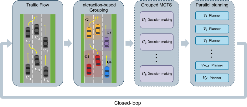
Figure 1: The architecture of TrafficMCTS. The yellow arrows indicate the driving intentions of each vehicle.

III Overview

III-A Problem Formulation

We first clarify the setup and goal of the vehicle traffic flow generation problem. Let $\mathcal{E}$ denote the scenario through which the traffic flow is traveling. Suppose there are $n$ vehicles inside scenario $\mathcal{E}$ for our system to control, denoted as $\mathcal{V}=\{V_{1},V_{2},\cdots,V_{n}\},n>0$. Meanwhile, there could be $m$ vehicles driving independently in the scenario, which manipulated by other algorithms or controlled by humans, $m\geq 0$.

Routing information plays a crucial role in defining efficient routes for vehicles to reach their destinations while avoiding traffic congestion. It is assumed that routing information is available in the problem, and this information is used to establish a driving intention for each vehicle. The driving intentions can be classified into several types, as illustrated in Table I.

TABLE I: Driving intentions for vehicles.

Driving intention	Description
Keep_Lane	Maintain the current lane
Change_Lane_Left	Drive into the left lane
Change_Lane_Right	Drive into the right lane
Merge_In	Merge in from the ramp
Drive_out	Drive out into the ramp
Overtake	Overtake the vehicle ahead and return the current lane

The goal of the problem is to generate feasible trajectories for each vehicle $V_{i}\in\mathcal{V}$. These trajectories should follow the vehicles’ routing information and make lane-changings or turns where appropriate, so that all vehicles can travel long distances to reach their destinations. The vehicles in the traffic flow are required to avoid collisions with each other and drive independently. They should also exhibit diverse but reasonable social interaction behavior. Considering a vehicle $V_{i}\in\mathcal{V}$, $\mathbf{x}^{i}_{t}$ denotes its state at time $t$, such as position and heading angle, etc. A feasible trajectory of vehicle $V_{i}$ should:

• Be defined as $\pi_{i}=\left[\mathbf{x}^{i}_{0},\mathbf{x}^{i}_{1},\cdots,\mathbf{x}^{i}_{T}\right]$ , where $T$ is the total duration of simulation. The final state at the end of simulation $\mathbf{x}^{i}_{T}$ must on the vehicle’s destination or on its way to its destination.

• Satisfy the vehicle dynamics $\mathbf{x}_{t+1}^{i}=f\left(\mathbf{x}_{t}^{i},u^{i}_{t}\right)$, where $u^{i}_{t}$ is the control input at time $t$ of $V_{i}$, such as throttle and steering angle, and $f$ represents vehicle’s dynamic function.

• Not collide with each other at any time, $\textit{shape}\left(\mathbf{x}_{t}^{i}\right)\cap\textit{shape}\left(\mathbf{x}_{t}^{j}\right)=\emptyset,i\neq j,\forall t\in\left[0,T\right]$, where $\textit{shape}()$ denotes the curve function of the vehicle body.

III-B System Architecture

To solve the traffic flow generation problem mentioned above, we propose TrafficMCTS, a closed-loop traffic flow generation framework that considers different behavioral preferences among vehicles. As shown in Fig. 1, the architecture includes four key modules and they form a closed loop generation of traffic flow: scenario cognition based on driving intentions, interaction-based grouping, grouped MCTS, and parallel planning.

The TrafficMCTS framework takes as input the states of the entire traffic flow and the driving intentions of each vehicle. The core of the framework is first to make a rough but long-term joint decision for vehicles, followed by parallel trajectory planning based on that decision. However, the large number of vehicles in the traffic flow leads to a large search space and low computational efficiency for simultaneous joint decision-making. To address this, we propose a group-based MCTS method that divides the traffic flow into several decision groups based on the potential interaction of the vehicles. For each decision group, the vehicles make joint decisions without priority, and the decision order between groups is classified into two types: sequential and parallel. After this process, each vehicle possesses a decision based on its state, and the TrafficMCTS framework uses a parallel trajectory planner to generate an optimal trajectory that guarantees safety. Finally, the vehicle positions within the traffic flow are updated according to the planned trajectories, and the above steps are repeated to complete the closed loop of the traffic flow generation.

We first describe the details of the group-based MCTS approach in Section IV-A. Secondly, the closed-loop process of TrafficMCTS is more intricate than described above. It involves distinct closed-loop frequencies for the decision-making process and the planning process, which will be elaborated further in Section IV-B. In addition, the architecture of TrafficMCTS supports the setting of unique driving preferences for vehicles to increase the diversity of traffic flows, which will be further discussed in Section IV-C.

The source code of our proposed traffic flow generation framework is available as part of open-sourced project LimSim [23]. Please refer to github.com/PJLab-ADG/LimSim/tree/master/trafficManager/decision_maker.

IV Methodology

IV-A Group-based Monte Carlo Tree Search

Multi-vehicle decision-making is always a challenging problem, because as the number of vehicles increases, the computational performance and decision success rate decrease. To address this issue, we propose a novel approach that groups vehicles based on their interaction and makes decisions separately for each group. In this section, we first introduce the multi-vehicle MCTS algorithm, which can handle decision-making problem among multiple vehicles in traffic flow. We then describe our vehicle grouping design based on interaction analysis, which aims to reduce the computational complexity of the decision-making process. Finally, we present our approach to making decisions in groups, which enables each group to make MCTS decisions separately and efficiently.

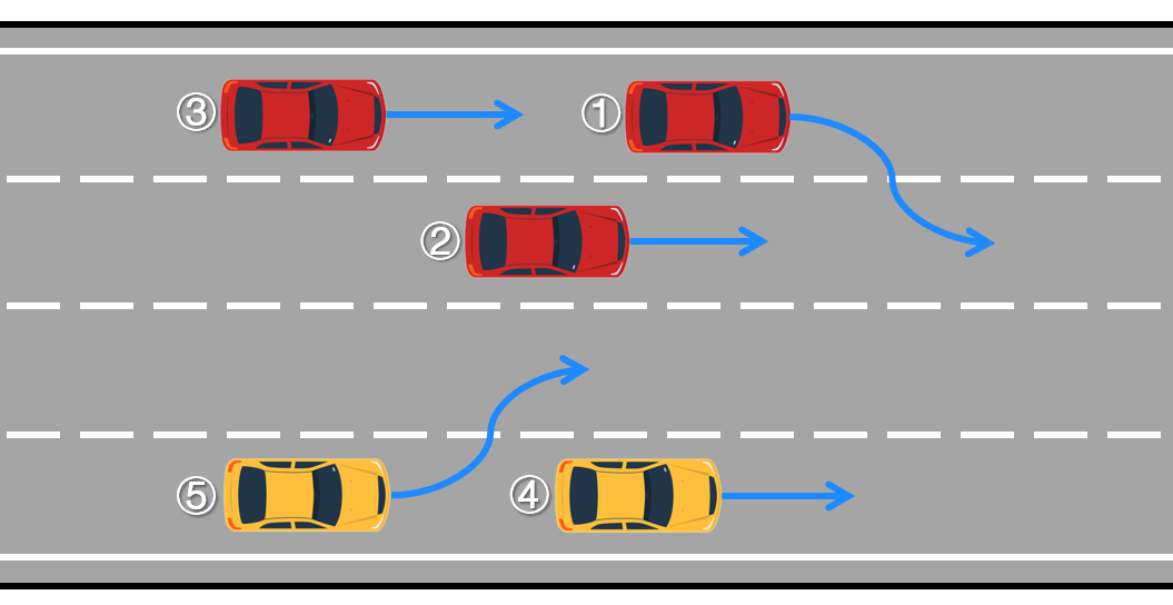
Figure 2: Schematic of the multi-vehicles with driving intentions in the highway scenario.

IV-A1 Multi-vehicle MCTS

The MCTS method can effectively solve the problems with huge exploration space. Starting from the initial node at $t=0$, the general MCTS algorithm performs $k$ iterations with four phases: selection, expansion, simulation, and back-propagation [35]. The selection phase adopts the UCT algorithm to address the exploration-exploitation dilemma. In the expansion phase, a collision check will be performed to prune the conflict child node. From a valid node, the algorithm uses a default policy to perform the simulation until it reaches a terminal node. In the back-propagated phase, the rewards from the simulation sample will be used to update the traversed nodes’ rewards. After a certain number of iterations, the search tree returns the node with the best reward. When applying the MCTS method to multi-vehicle joint decision-making, the prevailing methodology follows the approach of setting priorities for vehicles. Vehicles with higher priorities make decisions first, and those with lower priorities obey previous decisions.

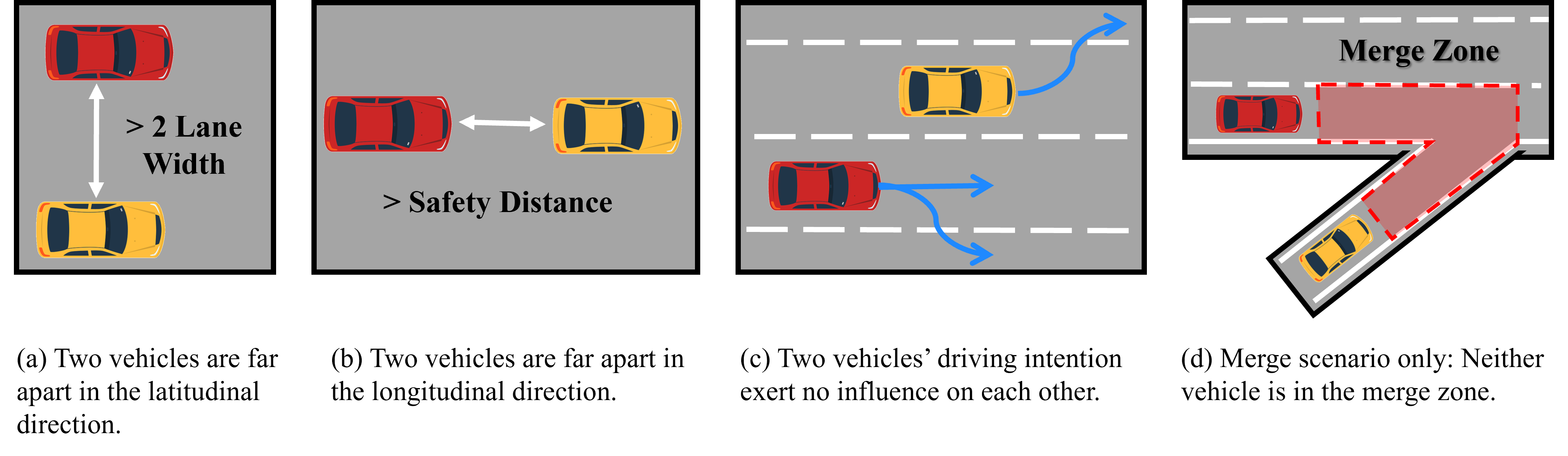
Figure 3: Cases in which vehicles are not considered to interact with each other.

TABLE II: Actions available for vehicles in one time step

Action	State change	Description
KS	$\left[v\Delta t,0,0\right]$	Maintain the current velocity
AC	$[v\Delta t+a_{acc}\Delta t^{2}/2,0,a_{acc}\Delta t]$	Increase the current velocity with a fixed acceleration $a_{acc}$
DC	$[v\Delta t-a_{dec}\Delta t^{2}/2,0,-a_{dec}\Delta t]$	Decrease the current velocity with a fixed deceleration $a_{dec}$
LCL	$\left[v\Delta t,-\Delta d,0\right]$	Make a partial left lane-changing with a width of $\Delta d$
LCR	$\left[v\Delta t,\Delta d,0\right]$	Make a partial right lane-changing with a width of $\Delta d$

In our previous work [36], we presented a multi-vehicle decision-making method based on the MCTS. This method eliminates the need for priority assignment during the decision-making process and effectively handles interactions between autonomous vehicles (AVs) and human-driven vehicles (HVs) in traffic flow. The method demonstrates robustness in dynamic environments while maintaining strong interpretability of the decision outcomes. To enhance its capabilities, we introduced the concept of metanode to replace the standard node in the general MCTS. This metanode enables the generation of simultaneous actions for multiple vehicles. As shown in Table II, there are five available actions for vehicles at each time step. At time step $t$, all controlled vehicles within the metanode select one of the five actions, while uncontrolled vehicles in the flow are assumed to perform a lane-keeping (KL) action. These chosen actions induce changes in the state of the traffic flow, leading to the formation of a new metanode. A terminal metanode indicates either all controlled vehicles within it have completed their intentions or that no feasible solution could be found within the decision period.

Using such a search method, all controlled vehicles can perform their intended driving actions based on the provided routing details, demonstrating impressive performance even in complex traffic scenarios. However, as the number of vehicles in the scenario increases, the search tree in the metanode of MCTS expands exponentially due to the joint consideration of all vehicles’ possible behaviors. Consequently, this expansion leads to a significant reduction in computational efficiency and overall success rate. To enhance the performance of the multi-vehicle MCTS algorithm for large-scale traffic flows in complex scenarios, additional measures should be taken to reduce the size of the solution space. We propose a novel group-based multi-vehicle decision-making method as below.

IV-A2 Vehicle Grouping based on Interaction Analysis

It is neither practical nor efficient to require each vehicle to be aware of all other vehicles, especially for vehicles that are too far apart to interfere with one another. For instance, considering the traffic flow depicted in Fig. 2. Vehicle 1, with the intention to change lanes to the right, will primarily interact with its neighboring vehicles 2 and 3 within a certain decision horizon. However, the available actions of vehicle 1, such as maintaining the current lane (AC) or executing a lane-changing to the right (LCR), have little effect on vehicles 4 and 5. Even in scenarios where human-driven vehicles (HVs) and autonomous vehicles (AVs) coexist, human drivers are limited by their visual perception and attention span, and they typically focus on the surrounding vehicles. This observation inspires us to divide the global interaction problem into a set of sub-problems. We partition the traffic flow into local groups based on the possibility of interaction, allowing for separate decision-making within each group. This approach enables us to maintain the benefits of the multi-vehicle MCTS algorithm, including high interpretability and interactivity, while significantly reducing the size of the solution space.

Several grouping methods have been developed to address the complexity of the joint multi-vehicle decision-making problem. Desiraju et al. divided the problem of maximizing safe lane-changings on an highway with multiple lanes into subproblems on a three-lane highway [37]. Within each subproblem, a grouping of vehicles is conducted based on the separation distances between vehicles, which were evaluated according to vehicles’ positions and speeds. Li et al. proposed a grouping method to meet the mandatory lane-changing demands for connected and automated vehicles [38]. This method primarily considered the distances between vehicles and imposes a maximum limit on the number of vehicles within each group. Although these approaches considered interactions between vehicles, they were limited to highway scenarios and can only make lane-changing decisions. Due to the simple grouping strategies, they did not fully exploit the potential benefits of grouping, leading to the over-filtering of feasible solutions.

In this paper, we propose a grouping algorithm based on interaction analysis, aiming to group vehicles that are likely to interact with each other into the same group whenever possible. This approach takes into account the vehicles’ intentions mentioned in Table I, allowing for a more refined assessment of the possibility of interaction between vehicles. The grouping method based on the interaction judgment goes beyond the highway scenario and offers a more reasonable solution. By utilizing the driving intentions derived from the routing information, the interaction between vehicles can be detected more accurately. We discuss the possibility of interaction between two vehicles $V_{i}$ and $V_{j}$ in the next several time steps. In some cases, they may not interact with each other, because they are far from each other or their actions taken based on their driving intentions will exert little influence on each other. These cases are summarized and listed in Fig. 3. Especially, the Merge Zone is defined as the section of the ramp and its nearest lane on the main road, extending a distance of $l$ ahead of the merge point. To avoid the potential collision in the next $k$ time steps, vehicles $V_{i}$ and $V_{j}$ should maintain the safety distance $s_{d}$, which is defined by

$$s_{d}\!=\!\begin{cases}\!&\!(v_{j}-v_{i})\!\cdot\!kt+\frac{1}{2}(a_{\text{acc}}+a_{\text{dcc}})\!\cdot\!(kt)^{2}+MSD,\\ &\!\quad\text{if }v_{j}\geq v_{i}\\ \!&\!MSD,\!\quad\text{if }v_{j}<v_{i}\end{cases}$$ (1)

where $MSD>0$ is constant, representing the minimum safe distance. This distance is calculated based on the assumption that the leading vehicle $V_{i}$ consistently performs a DC (Decelerate and Change lane) action with $a_{\text{dcc}}$, while the following vehicle $V_{j}$ consistently performs an AC (Accelerate and Continue in the same lane) action with $a_{\text{acc}}$ within the next $k$ time steps.

We use an adjacency matrix to record the information about the interaction possibilities between vehicles, which is called the interaction matrix. For a given traffic flow $\mathcal{V}$ consisting of $n$ vehicles, the interaction matrix $\Phi$ has a size of $n\times n$. Especially, if $\Phi_{i,j}=\Phi_{j,i}=1$, it indicates that vehicles $V_{i}$ and $V_{j}$ are likely to interact with each other. Conversely, if $\Phi_{i,j}=\Phi_{j,i}=0$, it suggests that there is no expected interaction between them. Since exchanging subscripts does not affect the determination of conflicting relationships, we only consider $\Phi_{i,j}$ in the following text and assume that $\Phi_{j,i}$ can be automatically updated with $\Phi_{i,j}$.

1 Initialize The interaction matrix $\Phi$ with all elements as 0;

2 $\mathcal{V}\leftarrow$ Sort vehicles by their longitudinal coordinates decreasingly;

3 for $V_{i}\leftarrow\mathcal{V}_{1}$ to $\mathcal{V}_{n}$ do

4       for $V_{j}\leftarrow\mathcal{V}_{i+1}$ to $\mathcal{V}_{n}$ do

             // Judge the relationship by the driving intentions

5             if $\left(V_{i},V_{j}\right){\rm\ in\ No\ Interaction\ Cases}$  then

6                   $\Phi_{i,j}\leftarrow 0$;

7            else

8                   $\Phi_{i,j}\leftarrow 1$;

9             end if

            // Overtaking intention requires additional consideration

10             if $\left(V_{i},V_{j}\right){\rm\ is\ an\ Overtake\ Pair}$  then

11                   $\Phi_{i,j}\leftarrow 1$;

12             end if

13            

14       end for

15      

16 end for

Result: The interaction matrix $\Phi$.

Algorithm 1 Judge_Interaction($\mathcal{V},\Psi$)

Algorithm 1 outlines the procedure for constructing the interaction matrix $\mathcal{V}$, which takes the vehicle flow $\mathcal{V}$ and the driving intentions $\Psi$ of the vehicles as input. The algorithm begins by sorting the flow in non-increasing order based on the vehicles’ longitudinal coordinates. This ensures that for any vehicles $V_{i}$ and $V_{j}$ in $\mathcal{V}$, if $i<j$, then $s_{i}\geq s_{j}$. It is important to note that since different lanes have different Frenét coordinate systems, all vehicles are converted to the same Frenét coordinate system by default in this algorithm. Next, starting from $V_{i}$, the algorithm determines whether $V_{i}$ and $V_{j}$ fall into any of the cases listed in Fig. 3. If a match is found, indicating no interaction between the vehicles, the corresponding element in the interaction matrix is set to 0. Otherwise, $\Phi_{i,j}$ are set to 1, indicating a potential interaction between the vehicles. It is important to highlight that an overtake pair, consisting of one vehicle with the intention to overtake and the other being overtaken, must be marked as having a possibility of interaction. This ensures that they can be grouped together later to facilitate the decision-making process for the Overtake intention.

1 $\textbf{Initialize}~{}\mathcal{V}_{1}.group\_idx\leftarrow 1$, $G_{1}\leftarrow\left\{V_{1}\right\}$, and $\mathcal{G}\leftarrow\left\{G_{1}\right\}$;

2 for $V_{i}\leftarrow\mathcal{V}_{2}$ to $\mathcal{V}_{n}$ do

       // Initialize the index of the group for $V_{i}$ as 0

3       ${V}_{i}.group\_idx\leftarrow 0$;

       // Reverse traversal to ensure adjacently grouping

4       for $V_{j}\leftarrow\mathcal{V}_{i-1}$ to $\mathcal{V}_{1}$ do

             // Do not be grouped together if the group is full

5             if ${\rm len}\left({G}_{V_{j}.group\_idx}\right)\geq N_{limit}$ then

6                   continue;

7             end if

            // Do not be grouped together if no interaction

8             if $\Phi_{i,j}$ is $0$ then

9                   continue;

10            else

                   // Put $V_{i}$ into the group to which $V_{j}$ belongs

11                   $V_{i}.group\_idx\leftarrow V_{j}.group\_idx$;

12                   $G_{V_{i}.group\_idx}\leftarrow G_{V_{i}.group\_idx}\cup\left\{V_{i}\right\}$;

13                   break;

14             end if

15            

16       end for

      // Form a new group

17       if $V_{i}.group\_idx$ is 0 then

18             $V_{i}.group\_idx\leftarrow{\rm len}(\mathcal{G})+1$;

19             $G_{V_{i}.group\_idx}\leftarrow\left\{V_{i}\right\}$;

20             $\mathcal{G}\leftarrow\mathcal{G}\cup\left\{G_{V_{i}.group\_idx}\right\}$;

21            

22       end if

23      

24 end for

Result: The grouping result $\mathcal{G}$ composed of several groups.

Algorithm 2 Grouping($\mathcal{V}_{s},\Phi$)

With the aid of the interaction matrix, the grouping of vehicles can be achieved, enabling us to efficiently solve the multi-vehicle decision-making problem. Algorithm 2 outlines the steps involved in the vehicle grouping process. The algorithm takes the sorted vehicle flow $\mathcal{V}$ and the interaction matrix $\Phi$ as input. The maximum number of vehicles allowed in a single group is limited to $N_{limit}$ to control the size of the search tree constructed for each group. The selection of the parameter $N_{limit}$ will be discussed later in Section IV-A3.

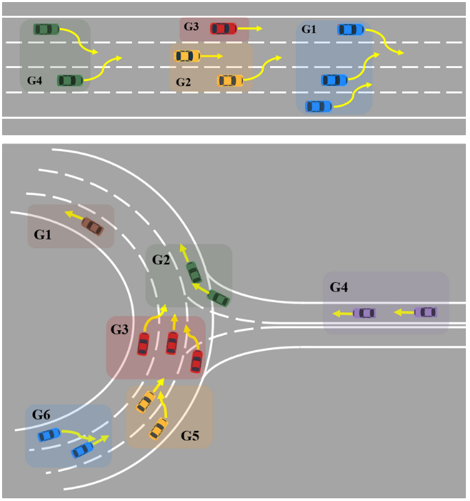
Figure 4: The results of grouping in freeway and roundabout scenario.

Algorithm 2 begins by initializing a group containing the first vehicle $V_{1}$ in $\mathcal{V}$. For each subsequent vehicle $V_{i}$, the algorithm iterates through the vehicles $V_{j}$ that are located in front of $V_{i}$, with $j$ ranging from $i-1$ to 1. Traversing from back to the front ensures that $V_{i}$ is grouped with its closest interacting vehicle. By examining the interaction matrix $\Phi$, if there is a possibility of interaction between $V_{i}$ and $V_{j}$, and the number of vehicles in the group to which $V_{j}$ belongs does not exceed $N_{limit}$, $V_{i}$ will be grouped with $V_{j}$. After the traversal, if $V_{i}$ has not been grouped yet, a new group will be created for it. The output of Algorithm 2 is a set of groups $\mathcal{G}$, where each group contains no more than $N_{limit}$ vehicles. It is worth noting that due to the limit of the maximum number of vehicles in a group, Algorithm 2 does not guarantee that vehicles with interaction possibilities are all grouped together. For two groups $G_{1}$and $G_{2}$ in $\mathcal{G}$, if there is no possibility of interaction between vehicles in $G_{1}$ and vehicles in $G_{2}$, the decision-making process can be conducted in parallel on them. Otherwise, the decision-making process should be sequential for them.

Fig. 4 illustrates the results of grouping in scenarios such as freeways and roundabouts. Our grouping algorithm takes into account detailed vehicle driving intentions, thus grouping vehicles that may interact with each other into the same group as much as possible. Moreover, vehicles without the possibility of interaction will be divided into different groups, which can improve computing efficiency through parallel decision-making and planning.

IV-A3 Making decision in Groups

Once the grouping process is completed, the decision-making process is conducted. As mentioned before, some groups can be considered in parallel, while others will make decisions in ascending order of group numbers. After Algorithm 2, the group with a smaller group number is located in front of the road segment. This decision-making order is reasonable since the preceding group has the initiative of passage and might have an impact on the following groups. If vehicle interaction exists in two adjacent groups, then the decision-making process of the following group should take the decision result of the preceding group into consideration; Otherwise, parallel decision-making is allowed for groups, where a sub-problem is created and the multi-vehicle MCTS method can be used separately for each group. Fig. 5 displays a traffic flow segmented into six distinct groups, Due to the interdependence of the vehicles in group 2 on the decisions made by group 1, a sequential approach to decision-making is essential. Similarly, sequential decision-making is required for vehicles in groups 3, 4, and 5. In contrast, vehicles in group 6 make decisions independent of the decisions of any other group, allowing it to engage in parallel decision-making alongside the above groups.

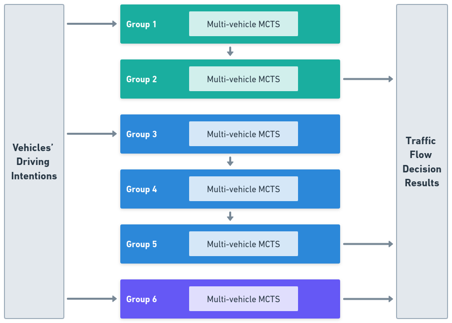
Figure 5: An example of making decision for a traffic flow with 6 groups of vehicles. Groups 1 and 2, as well as groups 3, 4, and 5, have inter-dependencies and require sequential decision-making. Group 6 has no inter-dependencies and can be directly decided upon. Therefore, group 6 can parallel perform decision-making simultaneously alongside group 1 and group 3.

For the $k$-th group in the sequential decision-making process, the multi-vehicle MCTS method takes the flow $\mathcal{V_{k}}$ as input, encompassing vehicles within the current group $G_{k}$ as well as those from all preceding groups $G_{1},G_{2},\dots,G_{k-1}$. The time taken by vehicle $V_{i}$ in the earlier flow to finalize its decision is denoted as $t_{i}$. As the tree expands up to time step $t$, actions and states of $V_{i}$ from the previous group’s decision results are directly retrieved if $t\leq t_{i}$. Conversely, if $t$ surpasses $t_{i}$, actions and states of $V_{i}$ are acquired from the prediction module. The states of all vehicles in the metanode are also obtained via the prediction module. Once the search tree concludes the decision-making for $G_{k}$, the outcomes and time steps for accomplishing driving intentions are documented. Following this, vehicles within $G_{k}$ are integrated into the previous flow. This iterative process persists until decisions are made for all groups within the sequential decision-making process.

Before utilizing the aforementioned approach for decision-making, it is crucial to determine the appropriate maximum vehicle number $N_{limit}$ within each group. We test the group-based MCTS algorithm in a freeway scenario containing a four-lane expressway to explore the effect of the selection of $N_{limit}$ on the algorithm performance. In this scenario, there are a total of 10 vehicles distributed across a 70-meter section, with at least six of them having the intention to change lanes. The decision module operates with a time step of 1.5 $s$, and the assessment of interaction possibilities considers the subsequent two time steps ($k=2$ in Eq. (1). The maximum of time steps is set as 10, which means that the search tree can expand up to the state at a maximum of 15 $s$. As $N_{limit}$ changes from 1 to 5, each test is repeated ten times under the same experimental setup. The results are shown in Fig. 6.

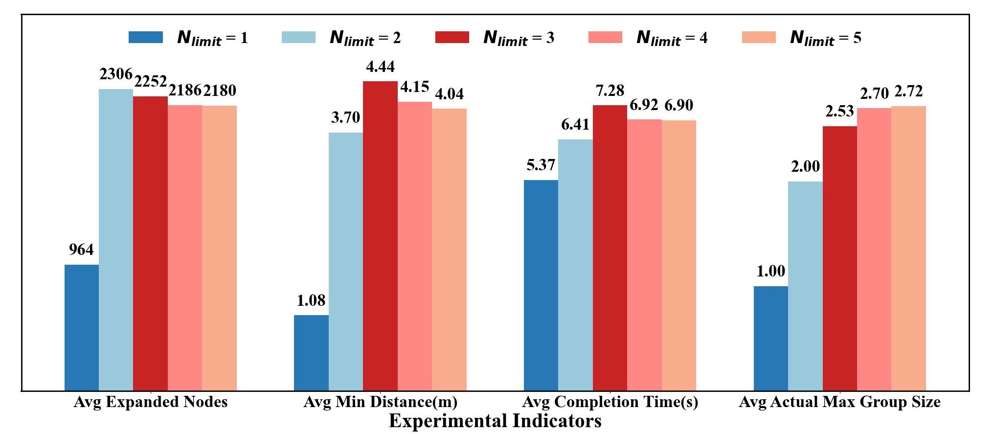
Figure 6: Experimental indicators of the test at different maximum group size limitation. The indicators in the horizontal axis (from left to right) are: (1) average expanded nodes in MCTS, (2) average minimum distance between vehicles, (3) average time taken for all AVs to complete their driving intentions, (4) average actual maximum size of the groups.

As $N_{limit}$ increases, the average number of expended nodes of the search tree increases firstly, then gradually decreases and tends to stabilize. Similarly, the average time taken for each group to complete their driving intentions follows the same trend. This can be attributed to the fact that when the number of vehicles in a group is small, especially when $N_{limit}=1$, the search tree terminates quickly. However, during the search process, interactions between vehicles are ignored, resulting in a very small average minimum distance between vehicles in the decision results. This means that the vehicles adopt extremely dangerous driving actions when completing their driving intentions. Furthermore, it is observed that as $N_{limit}$ increases, the average maximum number of vehicles in one group also increases but does not exceed 3. This indicates that setting $N_{limit}$ to 3 can meet the requirement for grouping those possible interacting vehicles together as much as possible. At the same time, indicators such as the average expansion nodes and the average minimum distance perform well at $N_{limit}=3$. Therefore, $N_{limit}$ is set to be 3 in our implementation of the group-based MCTS algorithm.

IV-B Closed-loop Decision-making and Planning

In this section, we focus on the closed-loop decision-making and planning process in our proposed framework. This process involves two key components: re-decision and replanning. These two components enable our framework to adapt to dynamic traffic scenarios and make real-time decisions and plans for safe and efficient traffic generation.

IV-B1 Re-decision

In Section IV-A, we propose a group-based MCTS method to generate long-term coarse decisions for large-scale traffic flows with complex interactions. The method consists of two main steps: grouping and multi-vehicle MCTS. The grouping algorithm focuses on the interactions between vehicles in certain time steps. However, for a flow dynamically changing, the interactions between vehicles also change constantly, so the grouping results need to be updated regularly. Furthermore, in some scenarios where the interactions between vehicles are complex, the group-based MCTS may not provide a feasible solution for all vehicles to complete their driving intentions within the decision interval. Therefore, re-decision is particularly necessary for the decision module to respond to the dynamic environment.

The interval of re-decision, denoted as $T_{update}$, plays a crucial role in the effectiveness of the decision-making process. If $T_{update}$ is too small, frequent updates of groupings and decisions may disrupt the vehicle’s execution of former decisions, leading to discontinuous driving behavior. This can lead to a reduced success rate for the flow in completing their driving intentions. Conversely, if $T_{update}$ is too large, the grouping results may no longer match the interactions between vehicles after several time steps. In this situation, the expansion node of the search tree cannot focus on handling the interaction between adjacent vehicles, which also reduces the search efficiency and decision success rate. A better choice is to make $T_{update}$ vary with the success rate of the decision results, instead of making it a fixed time interval. The decision success rate $\gamma$ refers to the ratio of the number of controlled vehicles completing their driving intention $N_{finish\_decision}$ to the number of controlled vehicles $N_{need\_decision}$. Mathematically, we difine that

$$\gamma=N_{finish\_decision}/N_{need\_decision}.$$ (2)

Then, we define the re-decision period $T_{update}$ as

$$T_{update}=T_{min}+\gamma\cdot\left(T_{max}-T_{min}\right),$$ (3)

where $T_{min}$ and $T_{max}$ represent the lower and upper limits of $T_{update}$, respectively. It indicates that when $\gamma$ is high, our framework tends to ensure that the vehicles can coherently execute the decision results. Conversely, when $\gamma$ is low, the loop can run frequently to find the feasible solutions as soon as possible in the dynamic environment.

In our group-based MCTS method, we check whether each controlled vehicle completes its driving intention. For a controlled vehicle $V_{i}$, if its driving intention is to change lane, merge or leave the main road, then the intention can be achieved when it is located in the target lane. If the intention is to overtake, it must also be ahead of the target vehicle $V_{aim}$ to complete the intention. For the vehicles successfully completing their driving intentions in a decision loop, the action sequences will be sent to the planning module to obtain the final feasible trajectories. Vehicles with the intention of keeping lanes or vehicles that have completed their intentions are keeping driving to provide trajectories for others until the end of the simulation.

IV-B2 Replanning

The planning module with a parallel architecture is proposed by [36] to generate continuous, kinematic-feasible, and collision-free trajectories. For each vehicle $V_{i}$ under our control, the single-vehicle trajectory planner receives an action sequence from the decision module. After predicting the future trajectories of other vehicles in the flow, it splits the different actions in the sequence and a sub-trajectory planner connects all trajectories for each action segment to obtain the final feasible and continuous vehicle trajectory.

The sub-trajectory planner expands the predefined constant state change described in Table II to form a continuous region of target states. In particular, for vehicles executing lane-keeping actions, particularly controlled vehicles that were unable to complete their driving intentions during the decision-making process, the planner generates a larger target state region to facilitate rational in-lane decisions. Subsequently, a set of target states is sampled within this predefined region.

We adopt quintic polynomial curves in the Frenét frame to generate the jerk-optimal connections between the start state and all sampled target states of the sub-trajectory. These alternative sub-trajectories are calculated with a cost function, which is detailed in Section IV-C2. The sub-trajectory with the lowest cost that satisfies the kinematic constraints and tests collision-free with other vehicles is selected, and the final state of this sub-trajectory is set as the initial state for the next sub-trajectory.

The above process is repeated in the fixed time interval $T_{planning}$ to avoid a potential collision. In each loop, the current state of $V_{i}$ will be set as the initial state for the next trajectory. In addition, the driving intention completion judgment mentioned in Section IV-B1 is conducted in every re-planning loop based on the vehicles’ current states. In this way, the driving intentions of the flow are updated timely when entering the next decision-making loop.

IV-C Generation of Diverse flow

One of the key objectives of our multi-vehicle decision-making and planning framework is to foster traffic flows with increased diversity. This is achieved by integrating the SVO [39] into the decision module and introducing the trajectory weight set within the planning module. By considering various cooperative tendencies and driving habits among vehicles and appropriately setting the SVO values and trajectory weight sets, we can effectively capture and reflect their individual characteristics. In this way, while attaching diversity to the flow, we can also control the behaviors of vehicles.

IV-C1 Decision Reward with SVO Embedded

During the simulation phase of group-based MCTS, the algorithm continues to select the valid metanode to extend the next time step until the simulation terminates. Then a reward will be calculated for this simulation from the result. We designed an embedded SVO reward function that guides vehicles to efficiently complete their driving intentions while characterizing their cooperative tendencies. Inspired by [39], the reward $R_{i}$ for $V_{i}$ in the traffic flow consists of reward to self $R_{self}$ and reward to other vehicles $R_{others}$, which are weighted by SVO angular preference $\varphi_{i}$. The definition of reward $R_{i}$ is shown as

$$R_{i}=\cos\left(\varphi_{i}\right)\cdot R_{self}+\sin\left(\varphi_{i}\right)\cdot R_{others},$$ (4)

where the orientation $\varphi_{i}\in[0,2\pi]~{}rad$. In the traffic flow, each vehicle would possess its unique factor $\varphi_{i}$. Some common definitions of the social preferences are

• Altruistic ($\varphi_{i}\approx\pi/2$): Maximize the others’ rewards, without consideration of their own outcomes.

• Prosocial ($\varphi_{i}\approx\pi/4$): Behave with benefiting the whole group and maximize the joint reward.

• Individualistic/egoistic ($\varphi_{i}\approx 0$): Maximize their own outcomes, without concern of others’ rewards.

The reward to self $R_{self}$ focuses on the efficient and safe completion of $V_{i}$’s driving intention, which includes two parts: the reward for the terminal state $R_{terminal}$ and the reward for the process states $R_{process}$. The former only concentrates on the leaf metanodes of the search tree, while the latter focuses on the path from the initial metanode to the terminal metanode.

$$R_{self}=R_{terminal}+R_{process},$$ (5)

where $R_{terminal}$ is exclusively acquired when $V_{i}$ completes its driving intention in the terminal metanode. $R_{process}$ is obtained by evaluating the state of the flow in each time step from multiple perspectives and adding them up. To improve travel efficiency, $V_{i}$ receives higher rewards when its speed approaches its target speed. To ensure rational driving behavior, $V_{i}$ receives higher rewards for continuous actions and staying on the center line of the lane. Furthermore, to enhance safety, $V_{i}$ receives higher rewards for maintaining a larger distance from its surrounding vehicles.

The reward $R_{others}$ is concerned with the interaction between $V_{i}$ and other vehicles in the flow. It is a negative value, i.e., it is the penalty caused by improper interactions. Improper interactions encompass actions such as recklessly lane-changing behavior, on-ramp vehicles rushing to merge into the main road, and main road vehicles refusing to yield to on-ramp vehicles. For $V_{i}$ with the intention of Overtake, Change_Lane_Left or Change_Lane_Right, it receives a penalty when its lane-changing actions force the rear vehicle in the target lane to decelerate. That is, $V_{i}$ chooses LCL or LCR action and the rear vehicle chooses DC action simultaneously in a metanode. Vehicles within the Merge Zone are also penalized if they perform improper interactions, such as on-ramp vehicles attempting to merge while main road vehicles refuse to yield.

After calculating $R_{self}$ and $R_{other}$, the reward $R_{i}$ for $V_{i}$ can be obtained by Eq. (4). It’s worth noting that the reward $R_{i}$ should meet in the range of 0 to 1. As the search tree in group-based MCTS handles all vehicles in the same group, the reward of the simulation is obtained by combining all rewards of vehicles within the terminal metanode as

$$R_{group}=\frac{1}{K}\underset{1\leq i\leq K}{\sum}R_{i},$$ (6)

where $K$ is the number of vehicles in the group and $R_{group}$ is the average reward of vehicles. Since $R_{i}\in[0,1]$, the distribution of $R_{group}$ is also guaranteed to stay in $[0,1]$. Finally, $R_{group}$ is used to update the average rewards of all traversed metanodes in the back-propagation phase.

IV-C2 Cost Function for Planning

The planner we employ bears resemblance to the one suggested by [40]. It employs uniform sampling of target states determined by the chosen action and generates jerk-optimal trajectories by utilizing quintic polynomial curves connecting the initial state to all the sampled target states. To assess the safety and comfort of each alternative trajectory, it is essential to calculate a corresponding cost function.

In particular, there are several cost terms for the vehicle $V_{i}$ in the function:

• Curve energy cost: $J_{i,cur}=\sum_{t\in\Gamma}\left(\kappa_{i}(t)\right)^{2}$, $\kappa_{i}(t)$ denotes the curvature of a point in the trajectory $\Gamma$. It penalizes the trajectory with sharp turns.

• Heading difference cost: $J_{i,\phi}=\sum_{t\in\Gamma}\left|\phi_{i}(t)-\phi_{r}\right|^{2}$,$\phi_{i}(t)$ denotes the orientation angle of the vehicle at a point in the trajectory $\Gamma$ and $\phi_{r}$ indicates the road’s direction at the point.

• Out of line cost: $J_{i,out}=\sum_{t\in\Gamma}\left|d_{i}(t)\right|^{2}$, $d_{i}(t)$ denotes the lateral offset in Frenét frame at a point in the trajectory $\Gamma$. This term is only active for actions except for lane-changing ones.

• Acceleration cost: $J_{i,acc}=\sum_{t\in\Gamma}\left(a_{i}(t)\right)^{2}$, $a_{i}(t)$ denotes vehicle’s acceleration at a point in the trajectory $\Gamma$.

• Jerk cost: $J_{i,jerk}=\sum_{t\in\Gamma}\left(j_{i}(t)\right)^{2}$, $j_{i}(t)$ denotes vehicle’s jerk (derivative of acceleration) at a point in the trajectory $\Gamma$. This term and the acceleration cost both contribute to the comfort of the trajectory.

• Dynamic obstacle cost: $J_{i,obs}$. This term serves to avoid the vehicle from being too close to the surrounding vehicles, which is described in detail below.

The dynamic obstacle cost takes into account the distance between a vehicle following a trajectory and dynamic obstacles on the road, such as surrounding vehicles. The cost for vehicle $V_{i}$ is defined as

$$J_{i,obs} = \sum_{t\in\Gamma}\sum_{\forall j\neq i}J_{i,obs}(t,j),$$ (7)

where $J_{i,obs}(t,j)$ represents the cost related to the position of vehicle $V_{j}$ relative to the current vehicle $V_{i}$ at time step $t$. In this study, we classify the position of vehicle $V_{j}$ relative to $V_{i}$ into three categories: 1) outside the alert zone; 2) inside the alert zone without collisions; 3) experiencing collisions with the current position of $V_{i}$. When vehicle $V_{j}$ is located outside the alert zone of $V_{i}$, it is considered safe and incurs no additional cost. Conversely, direct collisions with the trajectory of $V_{i}$ are deemed unacceptable. Within the alert zone, the cost increases as vehicle $V_{j}$ approaches closer to $V_{i}$.

The aforementioned terms are combined into a cost function as

$$J_{i} = \sum~{}w_{(\cdot)}~{}J_{i,(\cdot)},$$ (8)

where $J_{i,(\cdot)}\in\left\{J_{i,cur},~{}J_{i,\phi},~{}J_{i,out},~{}J_{i,acc},~{}J_{i,jerk},~{}J_{i,obs}\right\}$ represents the various cost components mentioned earlier, and $w_{(\cdot)}$ denotes the weight parameter corresponding to each cost component.

We observe that different drivers in a traffic flow may select different trajectories based on their driving preferences. In other words, drivers assign varying weights to these trajectory cost components. For example, some drivers may prioritize driving comfort, while others may prefer maintaining a greater safe distance from other vehicles. To account for this, we define a set of trajectory weights, denoted as $\mathcal{W}$, which includes $M$ weight vectors based on driver habits:

$$\mathcal{W}=\left\{\mathbf{w}_{1},\mathbf{w}_{2},\cdots,\mathbf{w}_{M}\right\}.$$ (9)

Each weight vector $\mathbf{w}_{k}\in\mathcal{W}$ contains a unique combination of weights for all the cost components, namely $\mathbf{w}_{k}=\left[w_{cur},~{}w_{\phi},~{}w_{out},~{}w_{acc},~{}w_{jerk},~{}w_{obs}\right]$. Each vehicle within the traffic flow individually selects a unique weight vector from the set $\mathcal{W}$ to generate its customized trajectories.

V Experiments

The simulation experiments are conducted to assess the performance of our proposed framework. First, a case study is presented to show the improvement of our group-based MCTS algorithm to other relevant approaches. Then, we illustrate how our closed-loop framework can bring diversity to AVs and manage the scenarios involving a mix of AVs and HVs. Finally, long-term simulations are conducted to demonstrate our framework’s ability to generate realistic large-scale traffic flows with complex interactions. In particular, a comparative experiment with SUMO displays the framework’s efficient decision-making ability in ramp scenarios.

In the first two experiments, the initial states of the vehicle flow is derived from real-world driving records obtained from the CitySim dataset [41]. Driving intentions such as lane-changings, entering or exiting ramps, and overtaking leading vehicles may be assigned to the vehicles. These driving intentions serve as inputs to the framework. The proposed framework is implemented under the environment of Python 3.10 on a PC with Intel Core i7-11700 @ 2.50GHz. To facilitate the discussion, the parameters of the vehicles in all experiments are listed in Table III. The time step is set to 1.5 $s$ in the decision module and 0.1 $s$ in the planning module. The grouping algorithm deals with interaction possibilities within the next two decision time steps. Besides, we set the minimum safe distance $MSD=2~{}m$ in Eq. (1). The maximum decision horizon is 9 $s$. In the closed-loop framework, the re-planning period is set to 0.3 $s$, and the lower and upper limits of the re-decision period are set to 1.5 $s$ and 6 $s$, respectively. For the sake of convenience, the weight of the cost function for vehicle planning remains unchanged across all experiments. The detailed experiment video can be found on YouTube with the URL of https://youtu.be/Tr0QWCasO54.

TABLE III: Parameters of the vehicles in the tests.

Symbol	Definition	Value
$w$	width of the vehicle	$2~{}m$
$l$	length of the vehicle	$5~{}m$
$a_{acc}$	acceleration for available actions	$0.6~{}m/s^{2}$
$a_{dec}$	deceleration for available actions	$0.6~{}m/s^{2}$
$\varphi$	SVO angular preference	$\pi/4~{}rad~{}\rm{(by~{}default)}$

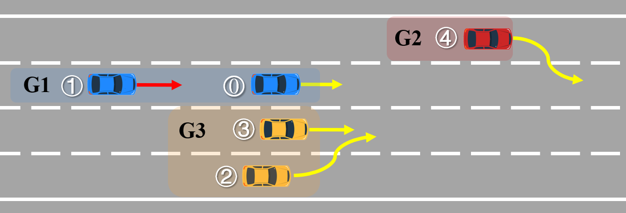
Figure 7: The four-lane freeway scenario of the test.

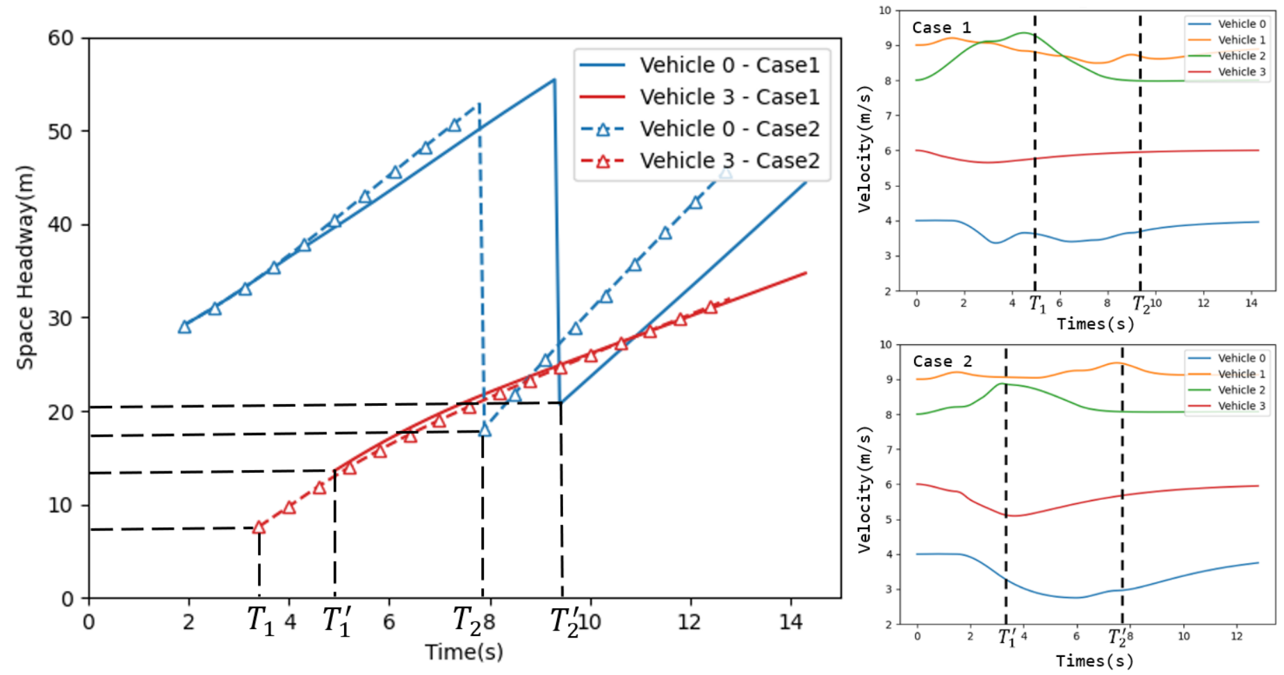
Figure 8: Distances to leading vehicles and the velocity profiles of certain vehicles in the test.

V-A Comparison of Method Performance

In this subsection, the performance of the group-based MCTS method is tested in a ramp scenario, which includes a three-lane main road with an on-ramp merging into it. All the vehicles in the traffic flow are controllable AVs. The number of AVs is set to 3, 6, and 9. To make the situation more complex, vehicles on the side lane of the main road will change lanes towards the middle lane, and vehicles on the middle lane are randomly assigned the driving intentions of Change_Lane_Right or Change_Lane_Left. The driving intentions of the on-ramp vehicles are Merge_in.

We use the sequential MCTS approach [30] as a comparison to evaluate the effectiveness of our proposed method. This method makes decisions for vehicles in order of priority within each decision time step. In this experiment, vehicles ahead possess a higher decision priority. The longitudinal acceleration in sequential MCTS is chosen from $\{1,0,1\}~{}m/s^{2}$, and the lateral velocity is chosen from $\{-1.2,0,1.2\}~{}m/s$. Moreover, to verify the effectiveness of the grouping algorithm, we also implement an MCTS approach based on the random grouping strategy. This approach does not take into account the possibility of interaction between vehicles during the grouping process. Instead, it assigns each vehicle a group index by randomly selecting a value between 1 and the total number of vehicles in the traffic flow $n$. It ensures that each group possesses at least one vehicle.

The time step and the maximum decision horizon are set the same for all three methods. Under different vehicle numbers, the maximum iteration number of MCTS is set to 2000, 4000, and 6000, respectively. For the group-based MCTS and the random-grouped MCTS, the sum of MCTS iterations for each group should not exceed the maximum iteration number. Each method is repeated ten times under the same experimental setup. The results of the decision-making method will be sent to the planning module with a planning horizon of 12 $s$ for all three methods. After that, the success rate of each method, the average number of expansion nodes in MCTS, the average number of available actions for each node in the search tree, the average time to finish the vehicles’ driving intentions, and the minimum inter-vehicle distance in the generated solutions are measured. The results are shown in Table IV.

TABLE IV: Comparative experiments with 3/6/9 vehicles in the ramp scenarios.

Method	Avg. Expanded Nodes	Avg. Available Actions for Each Node	Success rate (%)	Min. Distance $(m)$	Avg. Finish Time $(s)$
Sequential MCTS	$4924.7/9228.5/13033.2$	$167.3/91501.7/12674568.9$	$96.7/56.7/31.1$	$17.04/\textbf{5.07}/\textbf{3.62}$	$2.88/8.80/11.73$
Random-grouped MCTS	$2712.1/4137.1/5592.9$	$28.6/35.4/42.0$	$100.0/80.0/81.1$	$20.38/4.25/1.52$	$2.46/5.69/5.68$
TrafficMCTS	$\textbf{867.9}/\textbf{3001.2}/\textbf{3529.8}$	$\textbf{7.9}/\textbf{24.5}/\textbf{28.7}$	$\textbf{100.0}/\textbf{95.0}/\textbf{88.9}$	$\textbf{20.39}/4.25/2.45$	$\textbf{2.32}/\textbf{3.57}/\textbf{4.64}$

All three methods achieved high success rates in the ramp scenarios with three controlled AVs. However, when the number of AVs reaches 6, the success rate of the sequential MCTS method plummeted to $56.7\%$, and the random-group-based MCTS can only attain a success rate of $80\%$, while our method maintains a success rate of $95\%$. When $n$ reaches 9, the vehicle flow in the scenario is relatively congested and the interaction relationship is complex. Our method still manages to achieve a success rate of $88.9\%$, which is significantly better than the success rate of $31.1\%$ of the sequential MCTS method at this time. That is because the priority defined by sequential MCTS prevents higher-priority vehicles from yielding to the lower-priority vehicles, thereby filtering out some feasible solutions. On the other hand, as the number of vehicles increases, the search tree without grouping strategy grows exponentially, making it difficult to find a solution within a limited number of iterations.

The search efficiency can be reflected in the average number of expansion nodes. Under three sets of experimental parameters, our method is always the fastest to find a feasible solution among the three methods. Especially when $n=9$, under the same search iteration number limit, the sequential MCTS method expands nearly four times nodes than our method, but the success rate of its solution is far inferior to ours. By adopting the grouping strategy, the average number of available actions for each node maintains small with the increase in the number of vehicles. However, this indicator grows exponentially for the method without a grouping strategy. When $n=9$, this indicator of the sequential MCTS exceeds ten million, reaching an intolerable order of magnitude and leading to a huge decrease in search efficiency and success rate. Besides, compared to the random-group-based MCTS, the expansion nodes of our method focus on handling the interactions between adjacent vehicles. Therefore, even under the same order of magnitude of the average number of available actions for each node, our method can find a feasible solution faster.

In terms of the quality of the solutions, the average time for vehicles to complete their driving intentions is always the shortest in the solutions generated by our method. Meanwhile, the minimum inter-vehicle distances of our method are always good and hence ensure the safety of the vehicle flow. For $n=6$ and $n=9$, this value of our method is slightly smaller than that of the sequential MCTS. It is because in congested cases, the sequential MCTS often fails in decision-making and the vehicle defaults to keep driving in their current lane. But our method can still guide the vehicles safely to complete their lane-changing intentions. It is worth noting that the planning module refines the trajectory further, bringing all these three methods to collision-free trajectories.

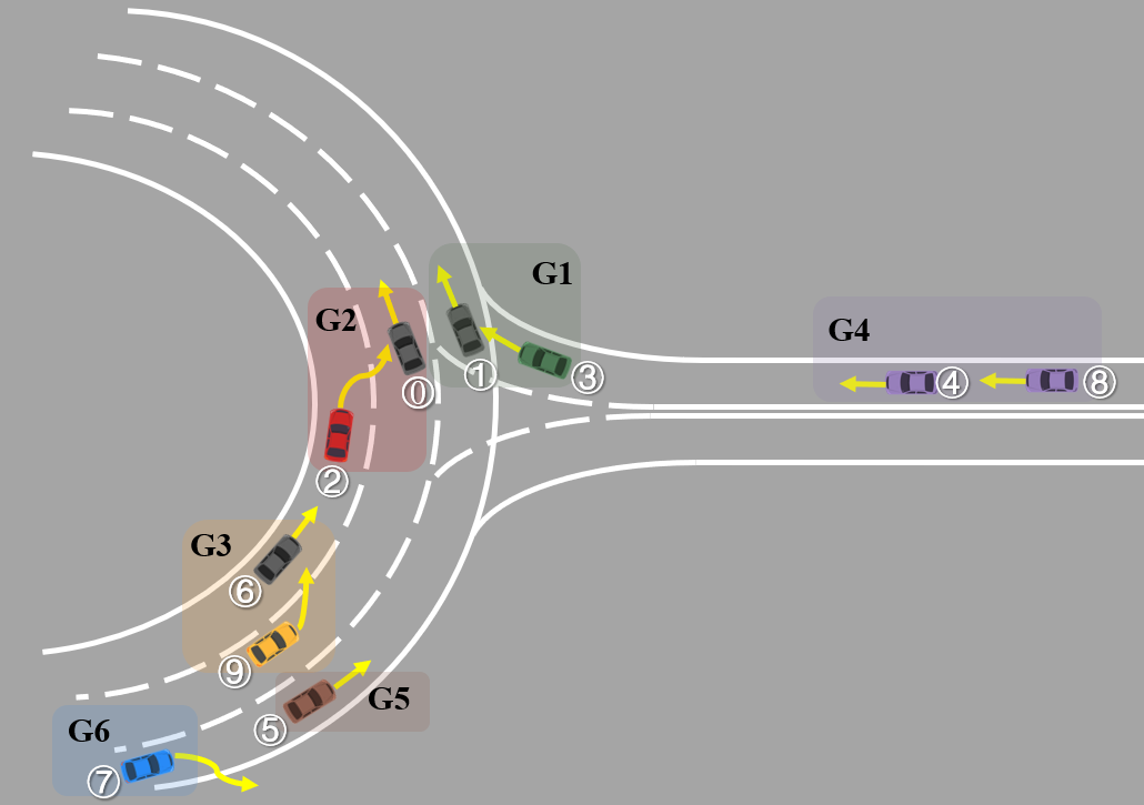
Figure 9: The roundabout scenario of the test.

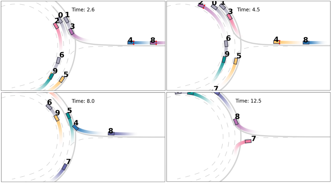
Figure 10: Snapshots of the simulation process for Roundabout-Case 1.

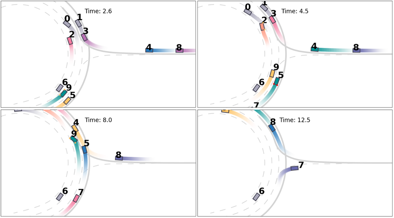
Figure 11: Snapshots of the simulation process for Roundabout-Case 2.

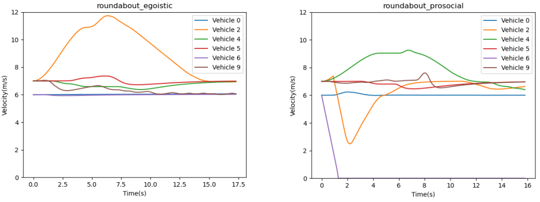
Figure 12: The velocity profiles of vehicle flow in the simulation process for Roundabout-Case 1 and 2.

V-B Illustration of Traffic Flow Diversity

We conduct several closed-loop simulations in the freeway and roundabout scenario to illustrate how our proposed framework can bring diversity to the vehicle flow at the social levels. Meanwhile, we demonstrate the framework’s ability to complete the Overtake driving intention and the responsiveness when facing other vehicles’ unanticipated actions.

V-B1 Four-lane Expressway

The first test scenario is shown in Fig. 7. In this freeway scenario containing a four-lane expressway, there are five AVs of $V_{i}~{}(i=0,1,2,3,4)$ controlled by our framework. $V_{0}$ and $V_{3}$ keep driving in their current lane. $V_{2}$ and $V_{4}$ intent to change to the adjacent lane. $V_{1}$ aims to overtake $V_{0}$. In the initial state of the vehicle flow, $V_{2}$ and $V_{3}$ are driving side by side in the adjacent lanes, so $V_{3}$ will interfere with $V_{2}$’s lane-changing intention. $V_{0}$ and $V_{1}$ constitute a overtake pair. Since $V_{4}$ is far away from $V_{0}$ and $V_{1}$, it does not affect the driving behavior of $V_{0}$ and $V_{1}$. The output of our grouping algorithm is consistent with the above analysis, which divides the vehicle flow into three groups: the first group only has $V_{4}$, the second group contains $V_{0}$ and $V_{1}$, and the third group contains $V_{2}$ and $V_{3}$.

In Freeway-Case 1, all the vehicles maintain their default SVO angular preferences with $\varphi_{i}=\pi/4~{}(i=0,1,2,3,4)$, which means they behave in a prosocial manner. In Freeway-Case 2, we change the manners of $V_{1}$ and $V_{2}$ to be egoistic with the SVO angular preferences modified as $\varphi_{i}=0~{}(i=1,2)$, whereas the other vehicles remain unchanged. The distances to leading vehicles (space headway) and the velocity profiles of $V_{0}$ to $V_{3}$ in each case are shown in Fig. 8. $T_{1}$ and $T_{2}$ indicate the moment $V_{2}$ and $V_{1}$ complete their driving intentions in Freeway-Case 1. $T_{1}^{\prime}$ and $T_{2}^{\prime}$ indicate the moment $V_{2}$ and $V_{1}$ complete their driving intentions in Freeway-Case 2. Thus, after $T_{1}$ and $T_{1}^{\prime}$, $V_{2}$ becomes the leading vehicle of $V_{3}$ through lane-changing; after $T_{2}$ and $T_{2}^{\prime}$, $V_{1}$ becomes the leading vehicle of $V_{0}$ through overtaking. It is shown that in Freeway-Case 1, $V_{1}$ and $V_{2}$ take more time to complete their driving intentions. Even though the speeds of $V_{0}$ and $V_{3}$ are relatively slow, $V_{1}$ and $V_{2}$ still choose to change their lanes after being far away from $V_{0}$ and $V_{3}$ to ensure safety and least influence on other vehicles. While in Freeway-Case 2, since $V_{1}$ and $V_{2}$ are only concerned about their rewards, the search trees provide the solutions for them to complete their driving intentions as quickly as possible. Thus, $V_{3}$ must slow down to make space for $V_{2}$ to complete its lane-changing at $T_{1}$, and $V_{1}$ does not accelerate that much as in Freeway-Case 1 to keep a large distance from $V_{0}$. Therefore, the velocities of $V_{0}$ and $V_{3}$ shown in Fig. 8 exhibit a rapid decrease, indicating that their driving behaviors are significantly influenced by $V_{1}$ and $V_{2}$.

TABLE V: Results of cases with different SVO settings for traffic flow diversity.

Case	Min. Space Headway $(m)$	Avg. Finish Time $(s)$	Max. Finish Time $(s)$	Avg. Flow Velocity $(m/s)$
Freeway-Case 1	$13.54$	$5.3$	$9.3$	$6.77$
Freeway-Case 2	$7.59$	$4.3$	$7.8$	$6.68$

The experimental indicators of the simulation process are shown in Table V, which are consistent with the above analysis. In Freeway-Case 2, the average time taken by vehicles to complete their driving intentions is shorter. However, due to the egoistic driving behaviors, the minimum distance between vehicles in the flow is smaller, which is prone to risks.

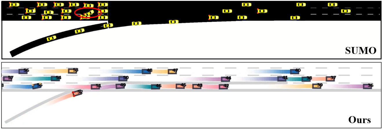
Figure 13: Snapshots of the simulation process at 58.0 $s$. The input traffic volume is set as 3600 $veh/h$.

V-B2 Unsignalized Three-lane Roundabout Entrance

The second test scenario is shown in Fig. 9. In this roundabout scenario with an unsignalized three-lane roundabout entrance, there are three uncontrolled HVs, $V_{0}$, $V_{1}$, and $V_{6}$. The remaining seven AVs are controlled by our framework. In the initial state of the vehicle flow, $V_{3}$, $V_{4}$, and $V_{8}$ are on the ramp and intent to merge into the main road. $V_{2}$ and $V_{5}$ are assigned with the driving intention of Change_Lane_Right and Change_Lane_Left respectively. $V_{7}$ is intent to exit the main road and enter the ramp. It should be mentioned that $V_{4}$ and $V_{5}$ almost simultaneously reach the intersection point of the main road and ramp, resulting in an interaction game between these two vehicles in the following time steps. Our grouping algorithm divides this initial flow into six groups.

In Roundabout-Case 1, all the HVs follow the predicted trajectories, which means they keep driving in their current lane. The SVO angular preference of $V_{5}$ is set as 0, and other vehicles maintain the default value, which means $V_{5}$ behaves in an egoistic manner. The traffic trajectories generated by our framework are shown in Fig. 10, where the controlled AVs in the flow are denoted by colored trajectories and uncontrolled HVs by grey trajectories. Except for HVs, vehicles with the same color belong to the same group. As shown in Fig. 10, the closed-loop experimental results show that $V_{2}$ and $V_{9}$ successfully complete their driving intentions in their interactions with HVs. Fig. 12 illustrates the change in the velocity of vehicles. Due to the slow speed of $V_{0}$ and the fact that the human driver does not slow down to make space for $V_{2}$, $V_{2}$ takes acceleration actions and completes the lane-changing after being far away from $V_{0}$. $V_{9}$ completes its lane-changing by slowing down and follows after $V_{6}$. As for the interaction game between $V_{4}$ and $V_{5}$, due to the egoistic driving behavior of $V_{5}$, it does not slow down to give way to $V_{4}$. Thus, $V_{4}$ decelerates in advance and follows behind $V_{5}$ after merging into the main road.

In Roundabout-Case 2, the driving behavior of $V_{4}$ is altered to be egoistic, and other vehicles maintain the default. Besides, we explore what happens when the uncontrollable HVs’ trajectories are inconsistent with the predicted trajectories input into the decision-making module. We modify the trajectory of $V_{0}$ to change to the left lane and bring $V_{6}$ an emergency stop, which simulates the abrupt lane-changing without a turn signal and sudden vehicle failure in the real scene respectively. Through the above case, the initial decision-making results will guide $V_{2}$ to accelerate and $V_{9}$ to turn left, creating quite dangerous situations.

The traffic trajectories generated by our closed-loop framework are shown in Fig. 11. Thanks to the high-frequency replanning in our planning module, $V_{2}$ and $V_{9}$ abort their original actions from the decision module when they realize that the adjacent vehicles do not cooperate with them to avoid the potential collision. $V_{2}$ performs a deceleration to make space for $V_{0}$, and continues to complete its lane-changing in the next decision-making loop. $V_{9}$ keeps its original lane, and changes to the left lane after being far away from $V_{6}$. As for the interaction game between $V_{4}$ and $V_{5}$, despite $V_{4}$’s backward initial position, to obtain higher rewards, $V_{4}$ accelerates to enter the Merge Zone first. Unlike Roundabout-Case 1, this time $V_{5}$ must yield to $V_{4}$. Thus, $V_{5}$ decelerates in advance and follows behind $V_{4}$ after $V_{4}$ merging into the main road.

The comparison between Roundabout-Cases 1 and 2 emphasizes the importance of integrating the planning module into the framework, which can quickly respond to changes in the road and resolve potential collisions between vehicles. Besides, the cases above demonstrate that by adjusting the vehicles’ social behaviors, our framework can bring interpretable diversity to the traffic flow and even generate extremely dangerous interaction scenarios.

V-C Long-term Closed-loop Simulation

With the help of the two-stage closed-loop modules, our framework ensures a real-time response to the dynamic environment, which is of great significance for long-term multi-vehicle simulation. In this subsection, we conduct a comparative experiment with SUMO [5] to display the efficient long-term decision-making ability of our framework. We also construct a road network containing multiple scenarios to demonstrate how our framework can be used to generate realistic large-scale traffic flows with complex interactions.

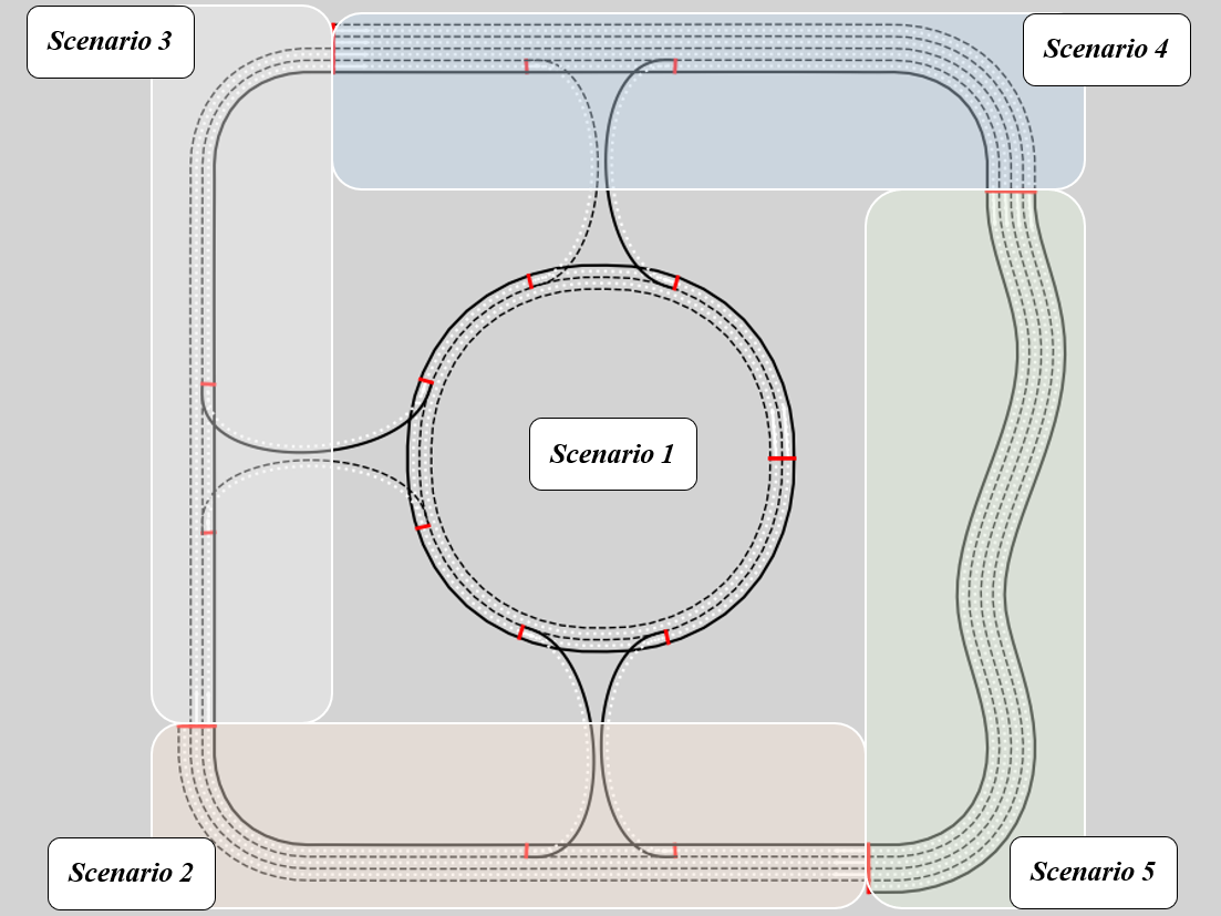
Figure 14: The road network containing five scenarios designed for the long-term large-scale traffic flows simulation.

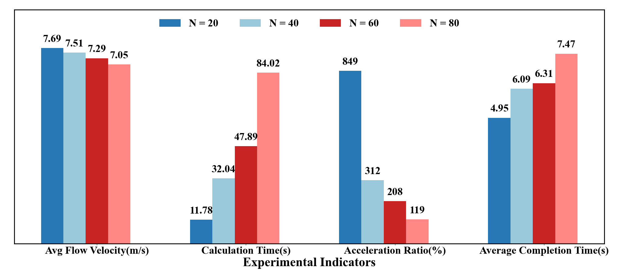
Figure 15: Experimental indicators of the simulation in the road network at different number of vehicles. The indicators in the horizontal axis (from left to right) are: (1) average flow velocity, (2) calculation time, (3) acceleration ratio, (4) average time taken for AVs to complete their driving intentions.

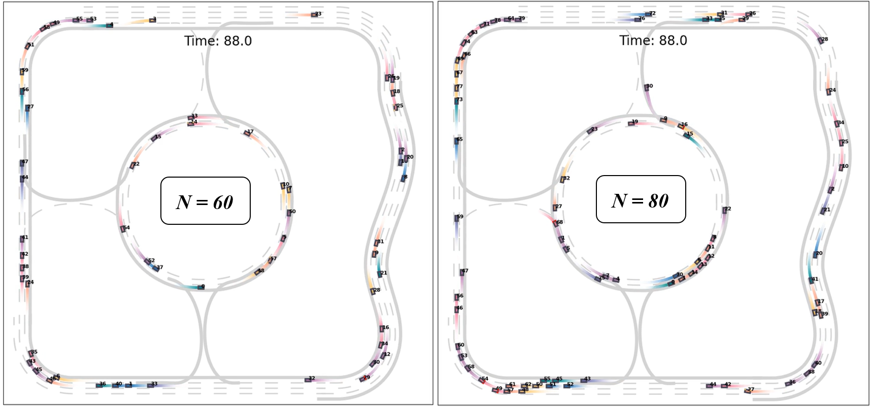
Figure 16: Snapshots of the simulation process at simulation time 88 $s$ with 60 and 80 vehicles.

V-C1 Comparison with SUMO

The first test is conducted in the same ramp scenario as Section V-A under different input traffic volumes. The traffic volume is set to 1800, 2400, and 3600 $veh/h$, which means that vehicles enter the scenario with time gaps of 2.0 $s$, 1.5 $s$, and 1.0 $s$, respectively. For a generated vehicle, it will randomly depart from the beginning of one of the three main road lanes or the ramp lane with the same probability. Its initial velocity is randomly and evenly selected from $[5,7]~{}m/s$, and its target speed is 9 $m/s$. The total length of the main road is 200 $m$, and the vehicles’ travel time is defined as the time they take from entering the scenario to arriving at the end of the main road. In addition, vehicles generated on the main road have the probability of 20% to be assigned the intention to change to the adjacent lane, thus constituting vehicle flow with complex interactions.

Besides the implement of our proposed framework, we also construct the above scenario in SUMO and generate vehicle routing information under different traffic volumes based on the above settings. Priority needs to be set for the main road and ramp in SUMO, which is an abstract ordinal number that determines right-of-way rules. We assign higher priority to the vehicles in the ramp by allowing vehicles to enter the main road as much as possible to ensure fairness. The longitudinal car-following model and the lateral lane-changing model of SUMO are the default. The simulation is implemented with SUMO 1.16.0. The total simulation time is 100 $s$.

TABLE VI: Results of the comparative experiment with SUMO.

Flow Volume $(veh/h)$	Avg. Flow Velocities $(m/s)$		Avg. Space Headway $(m)$		Avg. Travel Time $(s)$
	Ours	SUMO	Ours	SUMO	Ours	SUMO
1800	8.57	7.28	37.41	10.33	23.08	26.54
2400	8.57	4.84	34.73	7.89	22.87	34.03
3600	8.40	4.33	36.91	4.99	23.54	38.92

Table VI shows the the comparison between our framework and SUMO to simulate the same ramp scenario by several evaluating indicators. The results show that our framework outperforms SUMO in all experimental indicators under different input traffic volumes. In our framework, with the increase of the input traffic volume, the average vehicle velocity remains above 8.4 $m/s$, indicating that most vehicles achieve their target speed. Meanwhile, the average travel time keeps around 23 $s$ and the average space headway between vehicles maintains safe values. While in SUMO, when the traffic volume increases, the average vehicle velocity significantly decreases, resulting in longer average travel time. Average space headway between vehicles drops below 5 $m$, indicating a very congested and dangerous vehicle flow.

Fig. 13 shows the snapshots of the vehicle flow generated by SUMO and our framework under the input traffic volume of 3600 $veh/h$ when the simulation time is 58 $s$. The right-of-way priorities setting in SUMO requires that main road vehicles must stop waiting for on-ramp vehicles to merge into the main road, leading to congestion and even collision on the main road. Moreover, on the middle lane of the main road, the vehicle in the red circle performed a lane-changing trajectory that violated kinematics constraints and collided with another vehicle. By contrast, our framework offers flexible right-of-way priorities to vehicles in different lanes, avoiding unnecessary waiting of vehicles on the main road, thereby generating a more realistic and interpretable vehicle flow.

V-C2 Large-scale Road Network

The second test is conducted in a road network containing five scenarios shown in Fig. 14. There is a two-lane roundabout with three entrances and exits in the center, which is labeled as Scenario 1. These entrances and exits connect to the three-lane, two-lane, and four-lane expressways, respectively, which are labeled as Scenario 2, 3 and 4. Scenario 5 is a four-lane expressway connecting Scenario 2 and 4. There are two lane-drop bottleneck sections and six on-ramp merging sections in this road network.

Vehicles are generated in these five scenarios randomly to form the initial flow. Their initial velocities are randomly selected from $[6,8]~{}m/s$, and their target speeds are randomly selected from $[8,10]~{}m/s$. In the initial state, whenever a vehicle enters a new scenario, it will be assigned a driving intention randomly. For vehicles in the lanes of the main road of these five scenarios, their optional driving intentions include changing to the adjacent lane, overtaking the front vehicle and entering the ramp. It should be mentioned that the vehicles facing the lane-drop bottleneck are definitely intent to change to the right lane.

The simulation is conducted four times under different number of vehicles for 100 $s$. The vehicles’ average velocity and the average time to complete the driving intentions are analyzed to evaluate the performance of our framework. The results are presented in Fig. 15. As the number of vehicles increases from 20 to 80, the road network becomes congested, leading to the decrease of average velocity. And the interactions between vehicles become more and more complex, causing vehicles taking much time to complete their driving intentions. But the average velocity remains above 7 $m/s$ in all the tests, indicating that no severe congestion is formed in the simulation process. And the average time spent completing the driving intention keeps within a reasonable range, which is attributed to the closed-loop architecture of our framework. Even if the decision-making fails in certain complex scenarios, subsequent re-decision and re-planning procedures can always help the vehicle efficiently complete its decision intention. We also present the actual calculation time to generate the trajectories of the vehicle flows. The acceleration ratio in Fig. 15 refers to the ratio of simulation time to the calculation time. By adopting the group-based MCTS algorithm, our framework achieves high computational efficiency in large-scale traffic flow.

The snapshots of the simulation process are provided in Fig. 16. All the tests generate long-term and collision-free trajectories successfully, which can be used to generate the diverse traffic flows for various scenarios. Since all the vehicles actions are interpretable and can be adjusted at both the social interaction and individual habit levels, our framework can also be utilized to perform data augmentation of the existing traffic datasets with various driving styles.

VI Conclusion

In this paper we present TrafficMCTS, a novel framework for generating realistic and diverse traffic flows in a closed-loop manner. Our framework employs a novel group-based MCTS method that enhances computational efficiency by grouping vehicles according to their interaction potential. Furthermore, our framework incorporates Social Value Orientation (SVO) to model the social preferences and behaviors of different vehicles. TrafficMCTS ensures that the generated traffic flows are safe, kinematic-feasible, and adaptive to dynamic environments. Through experiments, we have shown that our approach surpasses existing methods in terms of computing time, planning success rate, and intent completion time. Our framework can generate a real-time traffic flow with up to 80 vehicles on the road network running on a single thread. In the future, we expect TrafficMCTS to serve as a traffic flow generator for digital twins and interactive simulations of intelligent transportation systems.

References

- [1] B. Coifman and L. Li, “A critical evaluation of the Next Generation Simulation (NGSIM) vehicle trajectory dataset,” Transportation Research Part B: Methodological, vol. 105, pp. 362–377, 2017.
- [2] H. Caesar, V. Bankiti, A. H. Lang, S. Vora, V. E. Liong, Q. Xu, A. Krishnan, Y. Pan, G. Baldan, and O. Beijbom, “nuScenes: A multimodal dataset for autonomous driving,” in IEEE/CVF Conference on Computer Vision and Pattern Recognition (CVPR), 2020, pp. 11 621–11 631.
- [3] P. Sun, H. Kretzschmar, X. Dotiwalla, A. Chouard, V. Patnaik, P. Tsui, J. Guo, Y. Zhou, Y. Chai, B. Caine et al., “Scalability in perception for autonomous driving: Waymo open dataset,” in IEEE/CVF Conference on Computer Vision and Pattern Recognition (CVPR), 2020, pp. 2446–2454.
- [4] J. Barceló, Fundamentals of traffic simulation. Springer, 2010, vol. 145.
- [5] P. A. Lopez, M. Behrisch, L. Bieker-Walz, J. Erdmann, Y.-P. Flötteröd, R. Hilbrich, L. Lücken, J. Rummel, P. Wagner, and E. Wießner, “Microscopic traffic simulation using SUMO,” in International Conference on Intelligent Transportation Systems (ITSC), 2018, pp. 2575–2582.
- [6] P. Hidas, “Modelling vehicle interactions in microscopic simulation of merging and weaving,” Transportation Research Part C: Emerging Technologies, vol. 13, no. 1, pp. 37–62, 2005.
- [7] M. Zhu, X. Wang, and Y. Wang, “Human-like autonomous car-following model with deep reinforcement learning,” Transportation Research Part C: Emerging Technologies, vol. 97, pp. 348–368, 2018.
- [8] Y. Tong, L. Wen, P. Cai, D. Fu, S. Mao, and Y. Li, “Human-like decision-making at unsignalized intersection using social value orientation,” arXiv preprint arXiv:2306.17456, 2023.
- [9] A. Dosovitskiy, G. Ros, F. Codevilla, A. Lopez, and V. Koltun, “CARLA: An open urban driving simulator,” in Conference on Robot Learning, 2017, pp. 1–16.
- [10] Q. Zhang, Y. Gao, Y. Zhang, Y. Guo, D. Ding, Y. Wang, P. Sun, and D. Zhao, “TrajGEN: Generating realistic and diverse trajectories with reactive and feasible agent behaviors for autonomous driving,” IEEE Transactions on Intelligent Transportation Systems, vol. 23, no. 12, pp. 24 474–24 487, 2022.
- [11] D. Lenz, T. Kessler, and A. Knoll, “Tactical cooperative planning for autonomous highway driving using monte-carlo tree search,” in IEEE Intelligent Vehicles Symposium (IV), 2016, pp. 447–453.
- [12] J. F. Fisac, E. Bronstein, E. Stefansson, D. Sadigh, S. S. Sastry, and A. D. Dragan, “Hierarchical game-theoretic planning for autonomous vehicles,” in International Conference on Robotics and Automation (ICRA), 2019, pp. 9590–9596.
- [13] H. Fan, F. Zhu, C. Liu, L. Zhang, L. Zhuang, D. Li, W. Zhu, J. Hu, H. Li, and Q. Kong, “Baidu Apollo EM motion planner,” arXiv preprint arXiv:1807.08048, 2018.
- [14] Q. Sun, X. Huang, B. C. Williams, and H. Zhao, “InterSim: Interactive traffic simulation via explicit relation modeling,” in IEEE/RSJ International Conference on Intelligent Robots and Systems (IROS), 2022, pp. 11 416–11 423.
- [15] M. Fellendorf, “VISSIM: A microscopic simulation tool to evaluate actuated signal control including bus priority,” in Institute of Transportation Engineers Annual Meeting, vol. 32, 1994, pp. 1–9.
- [16] J. D. J. Lozoya-Santos, R. Morales-Menendez, and R. A. Ramírez Mendoza, “Control of an automotive semi-active suspension,” Mathematical Problems in Engineering, vol. 2012, p. 218106, 2012.
- [17] M. Tideman and M. Van Noort, “A simulation tool suite for developing connected vehicle systems,” in IEEE Intelligent Vehicles Symposium (IV), 2013, pp. 713–718.
- [18] S. Shah, D. Dey, C. Lovett, and A. Kapoor, “AirSim: High-fidelity visual and physical simulation for autonomous vehicles,” in Field and Service Robotics: Results of the 11th International Conference. Springer, 2018, pp. 621–635.
- [19] S. Suo, S. Regalado, S. Casas, and R. Urtasun, “TrafficSim: Learning to simulate realistic multi-agent behaviors,” in IEEE/CVF Conference on Computer Vision and Pattern Recognition (CVPR), 2021, pp. 10 400–10 409.
- [20] J. Ren, W. Xiang, Y. Xiao, R. Yang, D. Manocha, and X. Jin, “Heter-Sim: Heterogeneous multi-agent systems simulation by interactive data-driven optimization,” IEEE Transactions on Visualization and Computer Graphics, vol. 27, no. 3, pp. 1953–1966, 2019.
- [21] L. Bergamini, Y. Ye, O. Scheel, L. Chen, C. Hu, L. Del Pero, B. Osiński, H. Grimmett, and P. Ondruska, “Simnet: Learning reactive self-driving simulations from real-world observations,” in IEEE International Conference on Robotics and Automation (ICRA), 2021, pp. 5119–5125.
- [22] C. Wu, A. Kreidieh, K. Parvate, E. Vinitsky, and A. M. Bayen, “Flow: Architecture and benchmarking for reinforcement learning in traffic control,” arXiv preprint arXiv:1710.05465, vol. 10, 2017.
- [23] L. Wen, D. Fu, S. Mao, P. Cai, M. Dou, and Y. Li, “LimSim: A long-term interactive multi-scenario traffic simulator,” arXiv preprint arXiv:2307.06648, 2023.
- [24] M. Montemerlo, J. Becker, S. Bhat, H. Dahlkamp, D. Dolgov, S. Ettinger, D. Haehnel, T. Hilden, G. Hoffmann, B. Huhnke et al., “Junior: The stanford entry in the urban challenge,” Journal of field Robotics, vol. 25, no. 9, pp. 569–597, 2008.
- [25] C. Urmson, J. Anhalt, D. Bagnell, C. Baker, R. Bittner, M. Clark, J. Dolan, D. Duggins, T. Galatali, C. Geyer et al., “Autonomous driving in urban environments: Boss and the urban challenge,” Journal of field Robotics, vol. 25, no. 8, pp. 425–466, 2008.
- [26] T. M. Howard and A. Kelly, “Optimal rough terrain trajectory generation for wheeled mobile robots,” The International Journal of Robotics Research, vol. 26, no. 2, pp. 141–166, 2007.
- [27] W. Ding, L. Zhang, J. Chen, and S. Shen, “EPSILON: An efficient planning system for automated vehicles in highly interactive environments,” IEEE Transactions on Robotics, vol. 38, no. 2, pp. 1118–1138, 2021.
- [28] P. Hang, C. Huang, Z. Hu, and C. Lv, “Driving conflict resolution of autonomous vehicles at unsignalized intersections: A differential game approach,” IEEE/ASME Transactions on Mechatronics, vol. 27, no. 6, pp. 5136–5146, 2022.
- [29] P. Cai, J. Zhang, X. Zhao, and Y. Li, “General driving behavior model based on the desired safety margin for vehicle flow simulation,” in International Conference on Intelligent Transportation Systems (ITSC), 2022, pp. 743–748.
- [30] C. Li, T. Trinh, L. Wang, C. Liu, M. Tomizuka, and W. Zhan, “Efficient game-theoretic planning with prediction heuristic for socially-compliant autonomous driving,” IEEE Robotics and Automation Letters, vol. 7, no. 4, pp. 10 248–10 255, 2022.
- [31] S. Casas, W. Luo, and R. Urtasun, “IntentNet: Learning to predict intention from raw sensor data,” in Conference on Robot Learning, 2018, pp. 947–956.
- [32] D. Chen and P. Krähenbühl, “Learning from all vehicles,” in IEEE/CVF Conference on Computer Vision and Pattern Recognition (CVPR), 2022, pp. 17 222–17 231.
- [33] Z. Peng, Q. Li, K. M. Hui, C. Liu, and B. Zhou, “Learning to Simulate Self-Driven Particles System with Coordinated Policy Optimization,” Advances in Neural Information Processing Systems, vol. 34, pp. 10 784–10 797, 2021.
- [34] Q. Sun, X. Huang, J. Gu, B. C. Williams, and H. Zhao, “M2I: From factored marginal trajectory prediction to interactive prediction,” in IEEE/CVF Conference on Computer Vision and Pattern Recognition (CVPR), 2022, pp. 6543–6552.
- [35] C. B. Browne, E. Powley, D. Whitehouse, S. M. Lucas, P. I. Cowling, P. Rohlfshagen, S. Tavener, D. Perez, S. Samothrakis, and S. Colton, “A survey of monte carlo tree search methods,” IEEE Transactions on Computational Intelligence and AI in games, vol. 4, no. 1, pp. 1–43, 2012.
- [36] L. Wen, P. Cai, D. Fu, S. Mao, and Y. Li, “Bringing diversity to autonomous vehicles: An interpretable multi-vehicle decision-making and planning framework,” in International Conference on Autonomous Agents and Multiagent Systems (AAMAS), 2023, pp. 2571–2573.
- [37] D. Desiraju, T. Chantem, and K. Heaslip, “Minimizing the disruption of traffic flow of automated vehicles during lane changes,” IEEE Transactions on Intelligent Transportation Systems, vol. 16, no. 3, pp. 1249–1258, 2015.
- [38] T. Li, J. Wu, C.-Y. Chan, M. Liu, C. Zhu, W. Lu, and K. Hu, “A cooperative lane change model for connected and automated vehicles,” IEEE Access, vol. 8, pp. 54 940–54 951, 2020.
- [39] W. Schwarting, A. Pierson, J. Alonso-Mora, S. Karaman, and D. Rus, “Social behavior for autonomous vehicles,” Proceedings of the National Academy of Sciences, vol. 116, no. 50, pp. 24 972–24 978, 2019.
- [40] M. Werling, J. Ziegler, S. Kammel, and S. Thrun, “Optimal trajectory generation for dynamic street scenarios in a frenet frame,” in IEEE International Conference on Robotics and Automation (ICRA), 2010, pp. 987–993.
- [41] O. Zheng, M. Abdel-Aty, L. Yue, A. Abdelraouf, Z. Wang, and N. Mahmoud, “Citysim: A drone-based vehicle trajectory dataset for safety oriented research and digital twins,” arXiv preprint arXiv:2208.11036, 2022.