Practical limitations on robustness and scalability of quantum Internet

Abstract

As quantum theory allows for information processing and computing tasks that otherwise are not possible with classical systems, there is a need and use of quantum Internet beyond existing network systems. At the same time, the realization of a desirably functional quantum Internet is hindered by fundamental and practical challenges such as high loss during transmission of quantum systems, decoherence due to interaction with the environment, fragility of quantum states, and other factors. We study the implications of these constraints by analyzing the limitations on the scaling and robustness of the quantum Internet. Considering quantum networks, we present practical bottlenecks for secure communication, delegated computing, and resource distribution among end nodes. Motivated by the power of abstraction in graph theory (in association with quantum information theory), that allows us to consider the topology of a network of users spatially separated over long distances around the globe or separated as nodes within the small space over a processor or circuit within a same framework, we consider graph-theoretic quantifiers to assess network robustness and provide critical values of communication lines for viable communication over quantum Internet.

In particular, we begin by discussing limitations on the usefulness of isotropic states as a base for device-independent quantum key repeaters which otherwise could be useful for device-independent quantum key distribution. We consider some quantum networks of practical interest, ranging from satellite-based networks connecting far-off spatial locations to currently available quantum processor architectures within computers, and analyze their robustness to perform quantum information processing tasks. Some of these tasks form primitives for delegated quantum computing, e.g., entanglement distribution and quantum teleportation, that are desirable for all scale of quantum networks, be it quantum processors or quantum Internet. For some examples of quantum networks, we also present algorithms to perform different quantum network tasks of interest such as constructing the network structure, finding the shortest path between a pair of end nodes for routing of resources, and optimizing the flow of resources at a node.

I Introduction

The quantum Internet Dowling and Milburn (2003); Kimble (2008); Wehner et al. (2018) is a network of users who are enabled to perform desired quantum information processing and computing tasks among them. Some of the important communication and computing tasks that we envision to be possible in full-fledged quantum Internet are cryptographic tasks against quantum adversaries of varying degree Bennett and Brassard (1984); Ekert (1991); Acín et al. (2007); Renner (2008); Barrett et al. (2013); Lucamarini et al. (2018); Arnon-Friedman et al. (2018); Das (2019); Xu et al. (2020); Das et al. (2021), quantum computation Shor (1994); Jozsa (1997); Grover (1996); Knill et al. (2001); Childs et al. (2003); Braunstein and van Loock (2005); Menicucci et al. (2006); Aaronson and Arkhipov (2011), distributed quantum computing Cirac et al. (1999); Fitzi et al. (2001); Raussendorf and Briegel (2001); Beals et al. (2013); Lim et al. (2005); Liu et al. (2023), delegated quantum computing Childs (2001); Giovannetti et al. (2008); Broadbent et al. (2009); Das and Siopsis (2021), quantum sensing Bollinger et al. (1996); Giovannetti et al. (2004, 2006); Budker and Romalis (2007); Taylor et al. (2008); Degen et al. (2017); Meyer et al. (2023), quantum clock synchronization Chuang (2000); Jozsa et al. (2000); Giovannetti et al. (2001), quantum communication Bennett and Wiesner (1992); Bennett et al. (1996a); Schumacher (1996); Mattle et al. (1996); van Enk et al. (1997); Bose (2003); Braunstein and van Loock (2005); van Loock et al. (2006); Zhang et al. (2017); Das et al. (2020); Kaur et al. (2019); Bhaskar et al. (2020); Cheong et al. (2022), superdense coding Bennett and Wiesner (1992); Mattle et al. (1996); Liu et al. (2002); Das and Wilde (2019), quantum teleportation Bennett et al. (1993); Bouwmeester et al. (1997); Furusawa et al. (1998); Horodecki et al. (1996); van Loock and Braunstein (2000), randomness generation and distribution Pironio et al. (2010); Colbeck and Kent (2011); Acín et al. (2012); Colbeck and Renner (2012); Yang et al. (2019), and others. Some of the crucial primitives for many of the quantum information and computing tasks are the distribution of resources like entanglement Schrödinger (1935); Braunstein and van Loock (2005); Horodecki et al. (2009a); Pan et al. (2012); Das et al. (2018a); Bäuml et al. (2018); Friis et al. (2019); Xing et al. (2023); Das et al. (2021); Khatri (2022a), nonlocal quantum correlations Bell (1964); Clauser et al. (1969); Brunner et al. (2014); Tavakoli et al. (2022); Aspect et al. (1982); Hensen et al. (2015); Giustina et al. (2015); Home et al. (2015); Braunstein and van Loock (2005); Luo (2022); Bjerrum et al. (2023), or quantum coherence Streltsov et al. (2015); Yao et al. (2015); Singh et al. (2021); Streltsov et al. (2017), etc.

Recent technological advancements have made it possible to realise quantum networks with fewer users at small distances Valivarthi et al. (2020); Wang et al. (2014); Stucki et al. (2011), however, the short lifetime of physical qubits (in some coherent states or quantum correlations) Ofek et al. (2016); Das et al. (2018b); Wang et al. (2022); Kim et al. (2023), the high loss experienced during the distribution of quantum systems across different channels Azuma et al. (2015); Ecker et al. (2022); Lu et al. (2022); Liu et al. (2022); Kaur et al. (2022); Das et al. (2021), and the use of imperfect measurement devices Briegel et al. (1998); Buscemi et al. (2016); Len et al. (2022); Sadhu and Das (2023); Das (2019) limits the realization of quantum networks for practical purposes. It is important to study the limitations of the quantum Internet, be it network connecting nodes in a quantum processor (or quantum computer) or network connecting users in different spatial locations to allow quantum information processing tasks among them. In this work, we use tools and techniques from graph (network) theory and quantum information theory to shed light on the limitations on the robustness and scalability of the quantum Internet.

Unlike classical signals, the losses associated with the transmission of quantum states between two parties via a lossy channel cannot be reduced by using amplifiers since the measurement will disturb the system Fuchs and Peres (1996) and unknown quantum states cannot be cloned Wootters and Zurek (1982). An alternative approach is to use quantum repeaters Briegel et al. (1998); Dür et al. (1999); Zhan et al. (2023) to enable entanglement distribution Das et al. (2018a); Wehner et al. (2018); Khatri et al. (2019); Shchukin and van Loock (2022) and perform cryptographic tasks Das et al. (2021); Xie et al. (2022); Horodecki et al. (2022); Li et al. (2023); Kamin et al. (2023); Li et al. (2022) over lossy channels. The quantum repeater-based protocols use entanglement swapping Zukowski et al. (1993); Pan et al. (1998); Bose et al. (1998); Sen (De) and optionally entanglement purification Bennett et al. (1996a); Deutsch et al. (1996); Bose et al. (1999); Hu et al. (2021) at intermediate points along the quantum channel. Advances in satellite-based quantum communication networks Ecker et al. (2022); Wang et al. (2021); Aspelmeyer et al. (2003); Bedington et al. (2017), improving system designs Śliwa and Banaszek (2003); Azuma et al. (2021); Bopp et al. (2022); You et al. (2022), and developing post-processing techniques Bennett et al. (1992a); Scarani and Renner (2008); Cai and Scarani (2009); Pearson (2004); Yin et al. (2020) are considerable efforts towards overcoming constraints on realizing the quantum Internet. With the assumption that some repeater-based schemes may improve the transmissivity of quantum channels connecting nodes in a network, we highlight instances to illustrate the limitations of current technology in implementing scalable quantum communication and DI-QKD networks.

If we focus on the topology of the quantum Internet, certain important questions arise: What is the effective structure of the underlying network to enable different parties to perform information processing tasks? Once a network structure is established, a significant concern is regarding its susceptibility to node and edge failures. A resilient network should possess the ability to carry out different information-processing tasks even if a substantial portion of its nodes becomes inactive. Consequently, it is desirable that the realization of the quantum Internet withstands the failure of a fraction of its nodes and links. This naturally leads to the question of how to evaluate the resilience of the quantum Internet and identify the nodes that are most crucial to its overall functioning. Having designed robust networks to enable different parties to perform desired information processing tasks, it is important to ask what strategies can be employed to optimize the flow of resources at the buffer nodes.

I.1 Motivation and main results

The power of abstraction in graph (network) theory West (2000); Tutte (2001) that provides a general formalism to analyze networks without getting into specific details of implementation Barnes and Harary (1983), motivates the use of graph-theoretic tools in analyzing the scalability and robustness of a global scale quantum Internet. Focusing on the robustness of networks, we present figures of merit for comparing different network topologies. We also apply ideas from percolation theory Broadbent and Hammersley (1957); Stauffer and Aharony (2018); Beffara and Sidoravicius (2005) to discuss the robustness of networks formed when performing a class of information processing tasks over any lattice network (sufficiently large graph).

One might find the level of abstraction quite high. However it is justified by the fact that we consider a system be it network or processor as the one after any technological improvement involving repeater techniques or fault tolerant quantum computing. No matter how they are defined, resulting output state will never be ideal but can only at best be close to ideal. For example, in some cases of practical interests, these final states can be modelled (in the case of links) as an isotropic state: ideal maximally entangled state mixed with the maximally mixed state (a useless noisy state) with some non-zero probability.

Considering the currently available quantum processors by Google AI (2021), IBM (2022) (2022); Begušić et al. (2023) and Rigetti Computing (2020) as real-world instances of graphical networks, we observe that the 54-qubit square topology of the Sycamore processor developed by Google AI (2021) has the highest node connection strength (see Fig. 1) and the lowest link sparsity. With the possibility of having a 1024-qubit quantum processor in the future, we extend the 54-qubit Sycamore processor layout to include 1024 qubits and present its figures of merit.

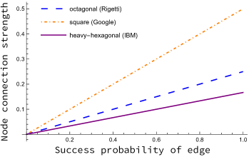
Figure 1: In this figure, we consider three processor designs by (a) Rigetti Computing (2020) (octagonal lattice), (b) Google AI (2021) (square lattice), and (c) IBM (2022) (2022); Begušić et al. (2023) (heavy-hexagonal lattice) as quantum networks and plot the connection strength of the nodes (see Eq. (31)) as a function of success probability of edge. It is assumed that the network have uniform distribution of edge success probability. (Color online)

The information-processing tasks that will be implemented using the quantum Internet will determine its structure. The building blocks for the structure of any network are the elementary links connecting two nodes of the network. It is therefore important to assess the limitations at the elementary link scale. To do this, we present the critical success probability of the elementary links for performing some desired information processing tasks. Extending to a more general repeater-based network with memory, we present a trade-off between the channel length and time spent at the nodes such that the state shared by the end nodes remains useful for various tasks.

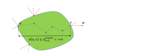
Figure 2: A network of point-to-point connections made of isotropic states is depicted. Any two nodes can be made directly connected via entanglement swapping to generate DI-QKD key along connecting path if and only if they are in a finite distance less than a critical one $\leq d_{crit}^{DIQKD}$. E.g. nodes $u$ and $w$ cannot be connected as they are too far. Only in the green area any pair of vertices can be made directly connected in device-independent way. In graph-theoretical language, the diameter of any fully connected subgraph is finite, bounded by $d_{crit}^{DIQKD}$. The same fact limits distance of connecting nodes with pure entanglement needed for faithful teleportation which enables e.g. delegated quantum computing. (Color online)

There is a strong motivation to enable remote places to securely access quantum processors via the quantum Internet and perform delegated quantum computing Childs (2001); Giovannetti et al. (2008); Broadbent et al. (2009) over the quantum Internet as it is less resource extensive on the individual user. To illustrate this, we may assume an instance where a user with limited computing resources in Bangalore requests to securely access the IBM Quantum Hub at Poznań Maciag-Kruszewska and ibmblogs via the quantum Internet. Enabling secure access requires the sharing of entangled states among distant nodes Das et al. (2018a); Halder et al. (2022); Khatri (2022a); Iñesta et al. (2023); Bugalho et al. (2023); Khatri (2021); Lee et al. (2022) along with performing secure cryptographic tasks against adversaries. We present limitations involved in implementing these tasks. In particular, we present limitations on using isotropic state Horodecki and Horodecki (1999) for distilling secret keys via DI-QKD protocols Ekert (1991); Acín et al. (2007) over the quantum Internet. We provide upper bounds on the number of elementary links between the end nodes for performing secure communication and information-processing tasks (see Fig. 2).

We show that a region of a (possibly infinite) network has a bounded size (graph-theoretically bounded diameter). Namely, any two nodes can be connected by entanglement swapping to produce a device-independent key by so-called standard protocols only if the nodes are closer to each other than the critical distance $d_{crit}^{DIQKD}$, which is always finite. It is a consequence of the recently discovered fact that even states exhibiting quantum non-locality may have zero device-independent key secure against quantum adversary Farkas et al. (2021). Our result can be phrased as no-percolation for DI-QKD networks in graph-theoretic language.

Let us recall here that we consider only the Bell measurements in the nodes since any technique improving the quality of the links, such as entanglement distillation or quantum error correction, is assumed to be performed beforehand.

Assuming there exists some scheme that can mitigate losses and improve transmittance over a quantum channel (see Assumption 1), we present limitations on the scalability of networks for performing quantum communication and implementing DI-QKD protocols. In particular, we present limitations on performing DI-QKD between two end nodes at a continental scale of distances and connected by repeater-based elementary links of metropolitan scale (see Example 1). Considering performing quantum communication over a lattice with optical fiber-based elementary links, we present limitations on its scalability (see Observation 2). These illustrate how far is the current technology from designing quantum networks for information processing tasks.

For long-distance communication over the continental scale of (order of $1000$ km) distances, the losses in transmission of optical signals over free space are significantly lower as compared to an optical fiber (see Fig. 28) making it better suited for distributing entangled states between far-off places. In this work, we present practical bottlenecks in realising such networks (see Fig. 17 and 18). As a potential application of the satellite-based network, we present the entanglement yield (see Fig. 21) and figures of merit of a global mesh network having $3462$ major airports across the globe as nodes and $25482$ airplane routes as edges connecting the major airports in the world. For such an airport network, we present the entanglement yield considering currently available and desirable technology available in the future. Looking at short-distance communication over the regional scale of (order of $100$ km) we present an instance of secure communication between a central agency and end parties. It may be desirable here for the central agency to prevent direct communication between the end parties. We consider a fiber-based star network for this task and present bottlenecks in its implementation (see Fig. 22).

To implement secure communication and share entanglement between the end nodes there are certain underlying network tasks that are needed to be performed. We present algorithms for implementing these network tasks. An important task is constructing the network structure to connect groups of network nodes. Once we obtain the network structure, we need the network path connecting two end nodes to enable the sharing of resources among them. In a general network, buffer nodes connecting multiple input and output channels may be present. The input channels may request to store resources at the buffer nodes while the output channels may request to extract resources stored in it. It is required to have a strategy to allocate resources to and from the buffer nodes in the network. We provide algorithms to perform these network tasks.

The structure of the paper is as follows. We introduce notations and review basic concepts and standard definitions in Sec. II. In Sec. III, we present limitations on using isotropic states in networks for device-independent secret key distillation. We present an upper bound on the number of elementary links between the end nodes such that the state shared by them remains entangled and is useful for different information-processing tasks. In Sec. IV, we analyze the robustness and scalability of the quantum Internet using graph (network) theoretic tools. Specifically, we present a graph theoretic framework for networks performing various tasks in Sec. IV.1 and present conditions for no percolation in a lattice network. In Sec. IV.2, we present the critical success probability of elementary links and critical length scales for various tasks over a repeater-based network. In Sec. IV.3, we present limitations on the scalability of networks for quantum communication assuming some hypothetical scheme can improve the transmission of channels connecting the nodes of the network. In Sec. IV.4 we present figures of merit to compare robustness of network topologies and in observe them for different networks in Sec. IV.5. In Sec. IV.6 we present measures to identify the critical nodes in a given network. In Sec. V, we present limitations on the potential uses of the quantum Internet for real-world applications. In particular, we present practical bottlenecks in the distribution of entangled states between far-off cities using a satellite-based network in Sec. V.1. Considering different quantum processor architectures as networks, we observe their figures of merit in Sec. V.2. In Sec. V.3, we first consider the task of connecting major airports across the globe via the satellite-based network and present the yield of the network. Then we present practical bottlenecks in connecting a central agency to the end parties via a star-based network. In Sec. VI, we present algorithms that are primitives for implementing different information-processing tasks using the quantum Internet. In particular, we consider the tasks of finding the shortest network path between a pair of nodes, resource allocation at a node with multiple input and output channels and constructing the network structure for connecting different end nodes. We provide concluding remarks in Sec. VII.

II Preliminaries

In this section, we introduce notations and review basic concepts and standard definitions that will be used frequently in later sections. We consider quantum systems associated with the separable Hilbert spaces. The Hilbert space of a quantum system $A$ and a composite system $AB$ are denoted as $\mathscr{H}_{A}$ and $\mathscr{H}_{AB}\coloneqq\mathscr{H}_{A}\otimes\mathscr{H}_{B}$ respectively. Let the dimension of the Hilbert space $\mathscr{H}_{A}$ be denoted as $|A|\coloneqq\dim(\mathscr{H}_{A})$. A quantum state of $A$ is represented by the density operator defined on $\mathscr{H}_{A}$. The density operator $\rho$ defined on $\mathscr{H}$ satisfies three necessary conditions: (i) $\rho\geq 0$, (ii) $\rho=\rho^{\dagger}$, (iii) $\operatorname{Tr}[\rho]=1$. A pure state is a rank-one density operator given by $\psi_{A}\coloneqq\outerproduct{\psi}{\psi}_{A}$ where $\ket{\psi}_{A}\in\mathscr{H}_{A}$. The set of density operators of $A$ is denoted by $\mathscr{D}(\mathscr{H}_{A})$. We denote the density operator of a composite system $AB$ as $\rho_{AB}\in\mathscr{D}(\mathscr{H}_{AB})$; $\operatorname{Tr}_{B}[\rho_{AB}]=\rho_{A}\in\mathscr{D}(\mathscr{H}_{A})$ is the reduced state of $A$. Separable states are those that can be expressed as a convex combination of product states

$$\rho_{AB}=\sum_{x}p_{x}\rho_{A}^{x}\otimes\rho_{B}^{x},$$ (1)

where $p_{x}\in[0,1]$ and $\sum_{x}p_{x}=1$. States that cannot be expressed in the form of Eq. (1) are said to be entangled. If $\rho_{AB}$ is an entangled state and one user has system $A$ and the user has system $B$, then we say that these two users share entangled pair.

A maximally entangled state of bipartite system $AB$ is defined as $\Psi_{AB}^{+}\coloneqq\outerproduct{\Psi^{+}}{\Psi^{+}}_{AB}$ where

$$\ket{\Psi^{+}}_{AB}=\frac{1}{\sqrt{d}}\sum_{i=0}^{d-1}\ket{ii}_{AB},$$ (2)

$d=\min\{|A|,|B|\}$ is the Schmidt-rank of the state $\Psi_{AB}^{+}$, and $\{\ket{i}\}_{i=0}^{d-1}$ forms an orthonormal set of vectors (kets). We next discuss families of states called isotropic states and Werner states.

Definition 1.

(Isotropic state Horodecki and Horodecki (1999)) An isotropic state $\rho_{AB}^{I}(p,d)$ is $U\otimes U^{\ast}$ invariant for an arbitrary unitary $U$. For $p\in[0,1]$, such a state can be written as

$$\rho_{AB}^{I}(p,d)\coloneqq p\Psi^{+}_{AB}+(1-p)\frac{\mathbbm{1}_{AB}-\Psi^{+}_{AB}}{d^{2}-1}$$ (3)

where $\Psi^{+}_{AB}$ is a maximally entangled state of Schmidt rank $d$. An Isotropic state $\rho_{AB}^{I}(p,d)$ written as in Eq. (3) is separable iff $p\in[0,1/d]$.

Remark 1.

We can also express isotropic states (Eq. (3)) as

$$\rho^{I}_{AB}\bigg{(}p(\lambda),d\bigg{)}=\lambda\Psi^{+}_{AB}+(1-\lambda)\frac{\mathbbm{1}_{AB}}{d^{2}}$$ (4)

for $p(\lambda)=[\lambda(d^{2}-1)+1]/d^{2}$ and $\lambda\in[-1/(d^{2}-1),1]$. We note that $\lambda^{n}\geq 0$ for all even $n\in\mathbb{N}$. For our purposes in this work, we will be restricting $\rho^{I}_{AB}\bigg{(}p(\lambda),d\bigg{)}$ to the case $\lambda\in[0,1]$ without loss of generality. We call $\lambda$ as the visibility of the state $\rho^{I}_{AB}\bigg{(}p(\lambda),d\bigg{)}$.

Definition 2.

(Werner state Werner (1989)) A Werner state $\rho_{AB}^{W}(p,d)$ is $U\otimes U$ invariant for an arbitrary unitary $U$. For $p\in[0,1]$, such a state can be written as

$$\rho_{AB}^{W}(p,d):=p\frac{2}{d(d+1)}\Pi_{AB}^{+}+(1-p)\frac{2}{d(d-1)}\Pi_{AB}^{-}$$ (5)

where $\Pi_{AB}^{\pm}:=(\mathbb{I}\pm F_{AB})/2$ are the projections onto the symmetric and anti-symmetric sub-spaces of $\mathscr{H}_{A}$ and $\mathscr{H}_{B}$. $F_{AB}=\sum_{ij}\ket{i}\bra{j}_{A}\otimes\ket{j}\bra{i}_{B}$ is the SWAP operator on $A$ and $B$. A Werner state $\rho_{AB}^{W}(p,d)$ written as in Eq. (5) is separable iff $p\in[1/2,1]$.

A quantum channel $\mathcal{M}_{A\to{B}}:\mathscr{D}(\mathscr{H}_{A})\to\mathscr{D}(\mathscr{H}_{B})$ is a completely positive, trace-preserving map. A measurement channel $\mathcal{M}_{A^{\prime}\to{AX}}$ is a quantum instrument whose action is defined as

$$\mathcal{M}_{A^{\prime}\to{AX}}(.):=\sum_{x}\mathcal{E}_{A^{\prime}\to{A}}^{x}(.)\otimes\outerproduct{x}{x}_{X},$$ (6)

where each $\mathcal{E}^{x}_{A^{\prime}\to{A}}$ is a completely positive, trace nonincreasing map such that $\mathcal{M}_{A^{\prime}\to{AX}}$ is a quantum channel and $X$ is a classical register that stores the measurement outcomes. A classical register $X$ is represented by a set of orthogonal quantum states $\{\outerproduct{x}{x}_{X}\}$ defined on the Hilbert space $\mathscr{H}_{X}$. We define qubit Bell measurement with success probability $q$ as

$$\mathcal{M}_{A_{1}A_{2}\to{X}}(.):= q\sum_{j=1}^{4}\operatorname{Tr}[\Psi^{(j)}(.)\Psi^{(j)}]\outerproduct{j}{j}_{X}$$ (7)

$$+(1-q)\operatorname{Tr}[.]\otimes\outerproduct{\perp}{\perp}_{X},$$

where $\{\Psi^{(j)}_{A_{1}A_{2}}\}_{j=1}^{4}$ denotes projective measurements on the set of maximally entangled states $\{\Psi^{+}_{A_{1}A_{2}},\Psi^{-}_{A_{1}A_{2}},\Phi^{+}_{A_{1}A_{2}},\Phi^{-}_{A_{1}A_{2}}\}$ (see Appendix B for details) and $\ket{\perp}\perp\ket{j}$.

Definition 3.

(Max-heap data structure Leiserson et al. (2009)) A max heap is a tree-based data structure that satisfies the following heap property: for any given node Y, if X is a parent of Y, then the key (the value) of X is greater than or equal to the key of Y.

In Fig. 3, we present the tree and array representations of a max heap data structure with $9$ nodes.

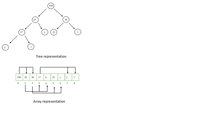
Figure 3: In this figure, we present the tree and array representations of a max-heap data structure with 9 nodes. In the tree representation, the nodes are shown in circles with the node values written inside them. In the array representation, the nodes are stored in continuous memory allocations (shown in green boxes numbered 0 to 9). The relation between the nodes is shown using arrows. We see that it satisfies the heap property: the value (or key) of a parent is always greater than its children. (Color online)

In the bipartite Bell scenario where there are two observables $\{x_{1},x_{2}\}$ for Alice and $\{y_{1},y_{2}\}$ for Bob, the family of tilted CHSH operators introduced in Acín et al. (2012) is given by

$$I_{\alpha}^{\beta}\coloneqq\beta~{}x_{1}+\alpha~{}x_{1}y_{1}+\alpha~{}x_{1}y_{2}+x_{2}y_{1}-x_{2}y_{2},$$ (8)

where $\alpha\geq 1$ and $\beta\geq 0$. The choice of $\beta=0$ and $\alpha=1$ corresponds to the CHSH operator Clauser et al. (1969). The local upper bound of the tilted CHSH operator is given by $\beta+2\alpha$. The quantum upper bound of the tilted CHSH operator is given by $2\sqrt{(1+\alpha^{2})(1+\frac{\beta^{2}}{4})}$.

Note 1.

In general, the logarithmic function can have base as the natural exponent $e$ or some natural number greater than or equal to $2$. In this paper, we consider the logarithmic function $\log$ to have base $2$ and natural logarithm $\ln$ to have base $e$ unless stated otherwise.

III Limitations on the network architecture with repeaters

A method for perfectly secure communication between a receiver and a sender requires sharing cryptographic keys between the parties Bennett and Brassard (1984). The secret keys can be shared between the receiver and the sender using quantum key distribution (QKD) protocols. For these protocols, the transmission of quantum states from one party to another is an important step. However, the transmission of quantum states from a sender to a receiver via a lossy channel inevitably degrades the state being transmitted. The overlap of the shared state with the intended state typically decreases monotonically with the length of the channel. Unlike a classical signal, for quantum states this loss cannot be reduced using amplifiers since the measurement will disturb the system Fuchs and Peres (1996) and also quantum states cannot be cloned Wootters and Zurek (1982). The degradation of the quantum states when transmitted over a quantum channel places limitations on the distance over which there can be secure communication Das et al. (2021). This limitation may be overcome by using entanglement-based QKD protocols Ekert (1991); Bennett et al. (1992b) along with quantum repeaters Briegel et al. (1998); Bäuml et al. (2015); Sangouard et al. (2011).

In classical computing, there is a strong motivation to use delegated computation in the form of cloud computing as it is less resource extensive on the individual user. Now, given that there is no full clarity regarding the path along which quantum computing will develop, delegated quantum computing Childs (2001); Giovannetti et al. (2008); Broadbent et al. (2009) is a vision aheadFitzsimons (2017). This vision has been supported by efforts to provide access to quantum processors over the Internet Steffen et al. (2016). The recent developments in the field of QKD and the current high-speed global communication networks only increase the scope for early adoption of delegated quantum computing.

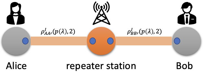
(a) Alice and Bob each send halves of isotropic state of visibility $\lambda$ to a repeater station which performs Bell measurement of the received qubits. After the Bell measurement, Alice and Bob share an isotropic state of visibility $\lambda^{2}$.

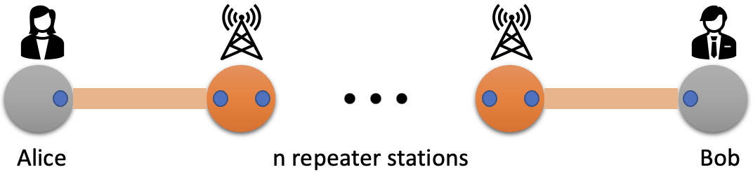
(b) Alice and Bob with n repeater stations in between them. After the repeater stations have performed Bell measurement, Alice and Bob share isotropic state of visibility $\lambda^{n+1}$.

Figure 4: In this figure, we present a repeater-based network to share isotropic states between Alice and Bob. The shared state is then used to perform DI-QKD protocols. The blue circles in the figure depict qubits. We assume all the repeater stations are equidistant and identical. (Color online)

Let us consider the task of sharing secret key between two distant parties over a repeater-based network. The parties say Alice and Bob each have two-qubit isotropic states given by $\rho_{AA^{\prime}}^{I}(p(\lambda),2)$ and $\rho_{BB^{\prime}}^{I}(p(\lambda),2)$ respectively and $\lambda\in[0,1]$. Alice and Bob send halves of their isotropic states to a repeater station. The repeater station performs a noisy Bell measurement on the halves of the isotropic states with success probability $q$ (see Fig. 4(a)). The action of the noisy Bell measurement is described by Eq. (66) (see Appendix C for details.) Assuming that error correction is possible post-Bell measurement, then from a single use of the repeater Alice and Bob with a probability $q$ share the two-qubit isotropic state

$$\rho_{AB}^{I}(p(\lambda^{2}),2)=\lambda^{2}~{}\Psi^{+}_{AB}+\frac{1}{4}(1-\lambda^{2})\mathbbm{1}_{AB}$$ (9)

of visibility $\lambda^{2}$ and $q$ being the success probability of performing the successful Bell measurement by the repeater station. The state $\rho_{AB}^{I}(p(\lambda^{2}),2)$ is separable if $\lambda\leq 1/\sqrt{3}$. All two-qubit states are entanglement distillable if and only if they are entangled Horodecki et al. (1998). All entanglement distillable states have non-zero rates for secret-key distillation Horodecki et al. (2009b). Alice and Bob can use the shared state $\rho_{AB}^{I}(p(\lambda^{2}),2)$ to perform a DI-QKD protocol based on the tilted CHSH inequality Acín et al. (2012) or the modified standard CHSH inequality Schwonnek et al. (2021). It was shown in Farkas et al. (2021) that for such protocols, the device-independent secret key distillation rate is zero when the visibility $\lambda^{2}$ of isotropic state $\rho_{AB}^{I}(p(\lambda^{2}),2)$ is below the critical threshold

$$\gamma_{\text{crit}}^{\theta}=\frac{\gamma_{L}^{\theta}+1}{3-\gamma_{L}^{\theta}},$$ (10)

where $\gamma_{L}^{\theta}=1/(\cos\theta+\sin\theta)$ and $\theta\in(0,\pi/2)$. The standard CHSH-based DI-QKD protocols use settings with $\theta=\pi/4$, which gives $\gamma_{\text{crit}}^{\pi/4}\approx 0.7445$. The DI-QKD rate is known to be non-zero for $\lambda^{2}\geq 0.858$ Acín et al. (2007). For $n$ repeater stations in between them (see Fig. 4(b)), Alice and Bob with probability $q^{n}$ share the two-qubit isotropic state

$$\rho_{AB}^{I}(p(\lambda^{n+1}),2)=\lambda^{n+1}~{}\Psi^{+}_{AB}+\frac{1}{4}(1-\lambda^{n+1})\mathbbm{1}_{AB}$$ (11)

of visibility $\lambda^{n+1}$ and $q$ being the success probability of performing a Bell measurement by the individual repeater stations. In the following proposition we present limitations on the use of isotropic states for distilling secret keys via DI-QKD protocols.

Proposition 1.

Consider the repeater relay network with an elementary link formed by node pair $\{v_{i},v_{j}\}$ and an intermediate repeater station. The nodes $v_{i}$ and $v_{j}$ share a two-qubit isotropic state $\rho_{ij}^{I}(p(\lambda^{2}),2)$. The end nodes of such a network share the state $\rho_{AB}^{I}(p(\lambda^{n+1}),2)$ of visibility $\lambda^{n+1}$ with probability $q^{n}$. For $\lambda\in(\sqrt{\gamma_{\text{crit}}^{\theta}},(\gamma_{\text{crit}}^{\theta})^{1/(n+1)})$, device-independent secret key distillation rate is zero among the end nodes even though $v_{i}$ and $v_{j}$ can distill device-independent secret keys at non-zero rate.

Proof.

The end nodes can use the shared state $\rho_{AB}^{I}(p(\lambda^{n+1}),2)$ to perform a DI-QKD protocol based on the tilted CHSH inequality Acín et al. (2012) or the modified standard CHSH inequality Schwonnek et al. (2021). The device-independent secret key rate for such protocols becomes zero for $\lambda^{n+1}\in(0,\gamma_{\text{crit}}^{\theta})$. This limits $\lambda$ to the range

$$\lambda\in\bigg{(}0,(\gamma_{\text{crit}}^{\theta})^{1/(n+1)}\bigg{)}$$ (12)

when no secret key can be distilled. For the elementary link formed by the node pair $\{v_{i},v_{j}\}$ having one repeater station between them, the key rate is zero for

$$\lambda\in\bigg{(}0,\sqrt{\gamma_{\text{crit}}^{\theta}}\bigg{)}.$$ (13)

It follows from Eq. (12) and (13) that for $\lambda$ in the range $\bigg{(}\sqrt{\gamma_{\text{crit}}^{\theta}},(\gamma_{\text{crit}}^{\theta})^{1/(n+1)}\bigg{)}$ the device-independent secret key distillation rate is zero for the end nodes even though end nodes of an elementary link of the network can distill secret keys at non-zero rates. ∎

For non-zero key rates from tilted CHSH inequality-based and the modified standard CHSH inequality-based DI-QKD protocols we require

$$n<\lfloor\frac{\log(1/\gamma^{\theta}_{\text{crit}})}{\log(1/\lambda)}-1\rfloor,$$ (14)

where $\lfloor.\rfloor$ denotes the floor function. For values of $n$ below the above threshold, we will have secure keys with a probability $q^{n}$. We plot in Fig. 5, the dependence of $n$ on $\lambda$ for performing DI-QKD protocol with non-zero key rate based on the tilted and modified standard CHSH inequality. In the plot, we have set $\gamma^{\theta}_{\text{crit}}$ to be 0.7445.

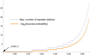
Figure 5: In this figure, we plot the allowed number of repeater stations and the success probability of performing a DI-QKD protocol with non-zero key rates by Alice and Bob as a function of the isotropic state parameter $\lambda$ when the critical threshold from Eq. (10) is $\gamma^{\theta}_{\text{crit}}=0.7445.$ (Color online)

In Fig. 5, we observe that the neighbouring nodes of a repeater chain network sharing a two-qubit isotropic state $\rho_{AB}^{I}(p(\lambda^{2}),2)$ with high visibility allows a large number of repeater stations between the end nodes for performing a DI-QKD protocol with non-zero key rates. However, the success probability of the DI-QKD protocol decreases with the increase in the number of repeater stations. In the bipartite scenario with two binary inputs and two binary outputs, there is a region where the device is nonlocal but has zero key Winczewski et al. (2022). Results similar to Proposition 1 and Eq. (14) would apply to such a scenario if considered appropriately.

We present in Appendix H bounds on the number of repeater stations such that the state shared by the end nodes of the network is useful for various information processing tasks. The repeater network discussed in this section can be generalised to a network structure with multiple pairs of end nodes.

Graph theory provides a framework to assess the topology of networks having spatially separated users across the globe, as well as networks with nodes within a small space over a processor or circuit without getting into specific details of implementation. Motivated by the power of abstraction, we analyze the robustness and scalability of the quantum Internet using graph theoretic tools in the following section.

IV Graph Theoretic analysis of networks

In this section, we first present a graph theoretic framework for networks. Using such a framework, we analyze the limitations on the scalability of repeater-based networks for different information processing tasks. Looking into the robustness of network topologies, we present tools for measuring network robustness and identifying the critical components. Using such measures, we compare the robustness of different network topologies.

IV.1 Graph theoretic framework of networks

Let us consider networks represented as graph $G(\mathbb{V},\mathbb{E})$ classified as weighted and undirected. A graph is a mathematical structure that is used to define pairwise relations between objects called nodes. The set of nodes, also called vertices is denoted by $\mathbb{V}$ and $\mathbb{E}$ denotes the set of edges which are pairs of nodes of the graph that connect the vertices. We denote $|\mathbb{V}|$ as $N_{v}$ and $|\mathbb{E}|$ as $N_{e}$, where $|\mathbb{X}|$ denotes the size of the set $\mathbb{X}$. The vertices of the graph $G$ are denoted as $v_{i}\in\mathbb{V}$ and the edges connecting the nodes $\{v_{i},v_{j}\}\in\mathbb{V}$ as $e_{ij}\in\mathbb{E}.$ We denote the path connecting two distant nodes $v_{i}$ and $v_{k}$ as ${\cal P}(v_{i},v_{k})$ having length $len(\cal P)$. The shortest shortest network path between $v_{i}$ and $v_{k}$ is denoted as $dist(v_{i},v_{k})$. The shortest path length between the most distant nodes of a graph is called the diameter of the graph. A value $w_{ij}\in\mathbb{R}$ assigned to an edge $e_{ij}$ of the graph is called the edge weight. The graph $G$ together with $w_{ij}$ is called a weighted graph. A graph where the edges do not have a direction is called an undirected graph. The edges of an undirected graph indicate a bidirectional relationship where each edge can be traversed from both directions.

In general, the nodes, edges, and edge weights of a network can change with time (see Appendix I for details). In this work, we will deal with undirected, weighted graphs depicting networks for communication tasks among multiple users. The edges in the graph are representative of links in the corresponding network, where links between nodes are formed due to quantum channels (or gates) over which resources are being transmitted between connected nodes. We denote labelled graphs as $G(\mathbb{V},\mathbb{E},\mathbb{L})$ where $\mathbb{L}$ denotes the set of labels associated with the vertices and edges of the graph.

We denote the nodes of the graph that are present between the end nodes when traversing along a path from one end node to another as the virtual nodes associated with the path. While analysing the network for different tasks, it may be possible that all the virtual nodes of the network are secure and cooperate in the execution of the task. We call this the cooperating strategy. It may also be possible that some virtual nodes of the network may be compromised and are not available for the task. We call this the non-cooperating strategy. We next define the weights for the edges of a network performing different tasks.

Definition 4.

Let a network depicted by an undirected, weighted graph $G(\mathbb{V},\mathbb{E})$, where $v_{i}\in\mathbb{V}$ for $i\in[N_{v}]$, be given by $\mathscr{N}(G(\mathbb{V},\mathbb{E}))$. The success probability of transmitting a desirable resource $\chi$ between any two different nodes $v_{i},v_{j}$ (i.e., when $i\neq j$) connected with edge $e_{ij}$ is given by $p_{ij}$; we assume $p_{ii}=1$ for an edge $e_{ii}$ connecting a node $v_{i}$ with itself. The weight $\mathrm{w}(e_{ij})$ for each edge $e_{ij}$ is given by $-\log p_{ij}$. We define an effective weight $\mathrm{w}_{\ast}(e_{ij})$ of an edge $e_{ij}$ over which the resource $\chi$ is transmitted between $v_{i}$ to $v_{j}$ for a particular information processing task ($\mathrm{Task}_{\ast}$) as, for all $i,j\in[N_{v}]$

$$\mathrm{w}_{\ast}({e_{ij}})\coloneqq\begin{cases}-\log p_{ij}&\text{if $p_{ij}\geq p_{\ast}$},\\ \infty&\text{otherwise},\end{cases}$$ (15)

where $p_{\ast}$ is the critical probability below which the desired information processing task ${\rm Task}_{\ast}$ fails. Since $G(\mathbb{V},\mathbb{E})$ is undirected, we have $p_{ij}=p_{ji}$, $\mathrm{w}(e_{ij})=\mathrm{w}(e_{ji})$, $\mathrm{w}_{\ast}(e_{ij})=\mathrm{w}_{\ast}(e_{ji})$.

Observation 1.

The weight $\mathrm{w}(e_{ij})$ for an edge is path-dependent and additive across connecting edges. If a resource $\chi$ is being transmitted between nodes $v_{i}$ and $v_{l}$ by traversing the virtual nodes $v_{j}$ and $v_{k}$ in an order $v_{i}\to{v_{j}}\to{v_{k}}\to{v_{l}}$, i.e., through a connecting path $e_{ij}\to{e_{jk}}\to{e_{kl}}$, then the weight $\mathrm{w}({e_{i\to{j}\to{k}\to{l}}})=\mathrm{w}(e_{ij})+\mathrm{w}({e_{jk}})+\mathrm{w}({e_{kl}})=-\log p_{ij}p_{jk}p_{kl}$. The effective weight $\mathrm{w}_{\ast}(e_{ij})$ is also path-dependent. The effective weight $\mathrm{w}_{\ast}({e_{i\to{j}\to{k}\to{l}}})=\mathrm{w}_{\ast}(e_{ij})+\mathrm{w}_{\ast}({e_{jk}})+\mathrm{w}_{\ast}({e_{kl}})=-\log p_{ij}p_{jk}p_{kl}$ if $p_{ij}p_{jk}p_{kl}\geq p_{\ast}$, else $\mathrm{w}_{\ast}({e_{i\to{j}\to{k}\to{l}}})=\infty$. If any of the $p_{ij},p_{jk},p_{kl}$ is strictly less than $p_{\ast}$ then $p_{ij}p_{jk}p_{kl}<p_{\ast}$. To maximize the success probability of transmitting the resource $\chi$ between any two nodes of the network, it is desirable to select the path between these two nodes that has the minimum weight.

The critical success probability for performing $\mathrm{Task}_{\ast}$ over a network limits its diameter. This motivates the following definition of critically large networks for $\mathrm{Task}_{\ast}$.

Definition 5 (Critically large network).

We define a network $\mathscr{N}_{\text{crit}}(G(\mathbb{V},\mathbb{E}))$ as critically large network for $\mathrm{Task}_{\ast}$ if

$$\forall_{e_{ij}\in\mathbb{E}}\,~{}p_{ij}\leq c,~{}\text{where}~{}c\in(0,1),$$ (16)

and it contains at least two vertices $x_{0},y_{0}\in\mathbb{V}$ which are at distance

$$dist(x_{0},y_{0})\geq\left\lceil\frac{\log p_{*}}{\log c}\right\rceil+1,$$ (17)

where $p_{\ast}$ is the critical probability for successful transmission of resource $\chi$ (Definition 4).

In the following proposition we show that there are at least two vertices in critically large network that cannot perform $\mathrm{Task}_{\ast}$ over all paths of length larger or equal to the distance between the vertices.

Proposition 2.

Assume that it is possible to perform ${\rm Task}_{\ast}$ between any two distinct nodes $v_{i},v_{j}$ of the network $\mathscr{N}_{\text{crit}}(G(\mathbb{V},\mathbb{E}))$ if and only if nodes $v_{i},v_{j}$ can share resource $\chi$ over the network path ${\cal P}(v_{i},v_{j})$ having success probability $s({\cal P}(v_{i},v_{j}))\geq p_{\ast}>0$. Then

$$\exists_{n_{0}<\infty}\forall_{\{v_{i},v_{j}\}\in\mathbb{V}}\, \bigg{[}dist(v_{i},v_{j})\geq n_{0}$$ (18)

$$\Rightarrow\forall_{{\cal P}(v_{i},v_{j})}\,\,s({\cal P}(v_{i},v_{j}))<p_{\ast}\bigg{]}.$$

In other words, there will be at least two vertices in this network, that cannot share resource $\chi$ by $\mathrm{Task}_{\ast}$.

Proof.

We begin with an observation that the success probability of sharing a resource between vertices $\{v_{i},v_{j}\}$ along the path ${\cal P}(v_{i},v_{j})$ is given by $s({\cal P}(v_{i},v_{j}))\coloneqq p_{ik}...p_{mj}$. The vertices $v_{i}$ and $v_{j}$ cannot share a resource along the path ${\cal P}(v_{i},v_{j})$ if $s({\cal P}(v_{i},v_{j}))<p_{\ast}$.

Let us choose $n_{0}$ such that $c^{n_{0}}<p_{\ast}$. Consider now any two vertices $v_{i}$ and $v_{j}$ be such that $dist(v_{i},v_{j})>n_{0}$ (the set of such vertices is non-empty since $dist(x_{0},y_{0})>n_{0}$ by assumption in Eq. (17)). Then any path ${\cal P}(v_{i},v_{j})$ has length $l\geq dist(v_{i},v_{j})$. The success probability of sharing resource along the path ${\cal P}(v_{i},v_{j})$ is given by $s({\cal P}(v_{i},v_{j}))=p_{ik}p_{kl}...p_{mj}\leq(\max\{p_{ik},p_{kl},...,p_{mj}\})^{l}\leq c^{l}\leq c^{n_{0}}<p_{\ast}$. Thus for any $\{v_{i},v_{j}\}$ at distance $\geq n_{0}$, there does not exist a path ${\cal P}(v_{i},v_{j})$ with $s({\cal P}(v_{i},v_{j}))\geq p_{\ast}$. ∎

Consider a $d$-dimensional lattice $G_{lat}(\mathbb{V},\mathbb{E})$ having $|\mathbb{V}|\rightarrow\infty$. The vertex set $\mathbb{V}$ is defined as the set of elements of $\mathbb{R}^{d}$ with integer coordinates. Let us denote $G_{sg}(\mathbb{V}_{sg},\mathbb{E}_{sg})$ as a finite subgraph of $G(\mathbb{V},\mathbb{E})$ from which the entire graph can be constructed by repetition and

$$\exists_{N_{sg}\ll|V|}:\forall_{v_{j}\in\mathbb{V}_{sg}}~{}\mathrm{degree}(v_{j})\leq N_{sg}.$$ (19)

A percolation configuration $\omega_{p}=(\omega_{ij}:e_{ij}\in\mathbb{E})$ on the graph $G(\mathbb{V},\mathbb{E})$ is an element of $\{0,1\}^{|\mathbb{E}|}$. If $\omega_{ij}=1$, the edge is called open, else closed. A configuration $\omega_{p}$ is a subgraph of $G(\mathbb{V},\mathbb{E})$ with vertex set $\mathbb{V}$ and edge-set $\mathbb{E}_{p}\coloneqq\{e_{ij}\in\mathbb{E}:\omega_{ij}=1\}$ (cf. Duminil-Copin (2018)). For performing $\mathrm{Task}_{\ast}$ over lattice network, we next present a theorem that describes conditions for which there is no percolation in a lattice network.

Theorem 1.

Let us consider performing $\mathrm{Task}_{\ast}$ (Definition 4) over the lattice $G_{lat}(\mathbb{V},\mathbb{E})$ where each edge is open with probability $p_{ij}$ and $0<p_{\ast}\leq p_{ij}<1$. Then the network arising among nodes from this task does not form a percolation configuration, i.e., a connected component of length $N_{c}$ such that $N_{c}/|\mathbb{V}|>0$.

The above theorem follows from the facts that there are periodic repetitions of the finite subgraph $G_{sg}(\mathbb{V}_{sg},\mathbb{E}_{sg})$ in $G_{lat}(\mathbb{V},\mathbb{E})$ and there exists at least two subgraphs whose distance is greater than critical threshold for inter-subgraph nodes to remain connected for $\mathrm{Task}_{\ast}$ with some desirable probability (see Proposition 2). See also (Stauffer and Aharony, 2018, Page 20) for discussion on 1-dimensional lattice and condition for percolation Beffara and Sidoravicius (2005) to exist. Theorem 1 implies limitations on the scalability of quantum communication (see Observation 2) and DI-QKD (see Example 1) over networks.

Let us next define the adjacency matrix and the effective success matrix of a network in terms of the success probability of transmitting a desirable resource $\chi$ between two nodes of the network.

Definition 6.

Consider a network $\mathscr{N}(G(\mathbb{V},\mathbb{E}))$ with $|\mathbb{V}|=N_{v}$ and ${\mathrm{w}(e_{ij})}_{i,j}$. The adjacency matrix $\mathbf{A}$ of the network is a $N_{v}\times N_{v}$ matrix such that for all $i,j\in[N_{v}]$ we have

$$[\mathbf{A}]_{ij}={\rm w}(e_{ij}),$$ (20)

and the effective adjacency matrix $\mathbf{A}_{\ast}$ of the network is given by

$$[\mathbf{A}_{\ast}]_{ij}={\rm w}_{\ast}(e_{ij}).$$ (21)

The effective success matrix of any network $\mathscr{N}(G(\mathbb{V},\mathbb{E}))$ for the transmission of a desirable resource $\chi$ (associated with ${\rm Task}_{\ast}$) between its nodes is an $N_{v}\times N_{v}$ matrix $\mathbb{f}_{\ast}$ such that for all $i,j\in[N_{v}]$ we have

$$[\mathbb{f}_{\ast}]_{ij}\coloneqq\begin{cases}p^{\rm max}_{ij}&\text{if $p^{\rm max}_{ij}\geq p_{\ast}$ for $i\neq j$},\\ 0&\text{otherwise},\end{cases}$$ (22)

where $p^{\rm max}_{ij}$ is the maximum success probability of transmitting the desirable resource $\chi$ between nodes $v_{i}$ and $v_{j}$ over all possible paths between the two nodes.

The elements $[\mathbb{f}_{\ast}]_{ij}$ of the success matrix provide the highest probability with which $\chi$ can be shared between the nodes $v_{i}$ and $v_{j}$ thus corresponds to the path having minimum cumulative effective weight. Let us consider a graph of diameter $2$ as shown in Fig. 6. The adjacency matrix and the success matrix for this graph are different as $[\mathbf{A}]_{14}=[\mathbb{f}_{\ast}]_{14}=0.79$ while $[\mathbf{A}]_{12}=0.198$ and $[\mathbb{f}_{\ast}]_{12}=0.54173.$ We observe that the success probability of transferring $\chi$ between nodes $v_{1}$ and $v_{2}$ via a non-cooperating strategy leads to a lower success probability $p_{1\to{2}}$ as compared to that via a cooperative strategy $p_{1\to{3}\to{2}}.$

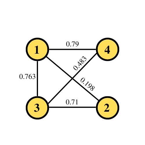
Figure 6: A partially connected mesh network with $4$ nodes. In this graph the adjacency matrix $\mathbf{A}$ and the success matrix $\mathbb{f}$ are different. While performing an information processing task using this network say transferring a resource $\chi$ from $v_{1}\to{v_{2}}$, it is preferable to use a cooperative strategy $v_{1}\to{v_{3}}\to{v_{2}}$ over a non-cooperative strategy $v_{1}\to{v_{2}}$ as it has a higher success probability. (Color online)

Note 2.

Henceforth, we will be dealing with communication over networks where the success probability of transmitting resources from a node $a$ to node $c$ via node $b$ is less than or equal to the multiplication of the success probability of resource transmission from $a$ to $b$ and $b$ to $c$.

IV.2 Limitations on repeater networks

In this subsection, we present the critical success probability of the elementary links for implementing different information processing tasks. Extending to a linear repeater-based network, we present the critical time and length scales for implementing different information processing tasks.

Critical success probability for repeater networks

Consider a network $\mathscr{N}(G(\mathbb{V},\mathbb{E}))$ for performing a particular information processing task denoted by the symbol $\mathrm{Task}_{\ast}$. As examples, we let the $\mathrm{Task}_{\ast}$ be sharing of entanglement, or implementing teleportation protocol between the nodes $\{v_{i},v_{j}\}\in\mathbb{V}$. Let $v_{i},v_{j}$ share an isotropic state given by

$$\rho_{ij}^{I}(p,d)=p_{ij}\Psi^{+}_{ij}+(1-p_{ij})\frac{\mathbbm{1}_{ij}-\Psi^{+}_{ij}}{d^{2}-1},$$ (23)

via a qudit depolarising channel (cf. Das et al. (2021); Kaur et al. (2022)). Following Eq. (15), let us denote $p_{\ast}$ as the critical success probability below which the task $\mathrm{Task}_{\ast}$ fails. The quantum state shared by nodes $v_{i}$ and $v_{j}$ become separable for $p_{ij}<1/d$, this implies a critical success probability $p_{\ast}^{\text{ent}}\geq 1/d$. The singlet fraction of the state shared between $v_{i}$ and $v_{j}$ is given by $f_{ij}=p_{ij}$. The maximum achievable teleportation fidelity of a bipartite $d\times d$ system in the standard teleportation scheme is given by $F=\frac{f_{ij}d+1}{d+1}$ Horodecki et al. (1999). The maximum fidelity achievable classically is given by $F_{cl}=\frac{2}{d+1}$ Horodecki et al. (1999). Thus the shared state between $v_{i}$ and $v_{j}$ is useful for quantum teleportation if $f_{ij}>1/d$. The critical success probability $p_{\ast}^{\text{tel}}$ for performing teleportation protocol over $\mathscr{N}(G(\mathbb{V},\mathbb{E}))$ is $p_{\ast}^{\text{tel}}>1/d$.

Critical time and length scales for repeater networks

Consider an entanglement swapping-based repeater network. Let there be two sources $S_{1}$ and $S_{2}$ producing dual-rail encoded entangled pairs (for details see Appendix A) in the state $\Psi^{+}$ with probability $\eta_{s}$ and with probability $1-\eta_{s}$ produces a vacuum state. The source $S_{1}$ sends one qubit from its entangled pair to Alice and the other to the repeater station via optical fibers of length $l$. Similarly, $S_{2}$ sends one qubit from its entangled pair to Bob and the other to the repeater station via optical fibers of length $l$ (see Fig. 7). Let the qubits be stored in quantum memories at the repeater station and the stations of Alice and Bob for time $t$.

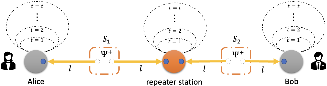
Figure 7: In this figure, we present an entanglement swapping-based repeater network. There are sources $S_{1}(S_{2})$ producing state $\Psi^{+}$ and sending it to a repeater station and Alice (Bob) via optical fibers of length $l$ (shown in yellow). The qubits are stored in quantum memories at the repeater station and the stations of Alice and Bob for $t$ time steps (shown as self-loops). The repeater station performs Bell measurement on its share of qubits. (Color online)

We model the evolution of the qubits through the fiber and at the quantum memory as a qubit erasure channel (see Sec. E.2) with channel parameter $\eta_{e}=\mathrm{e}^{-(\alpha l+\beta t)}$, where $\alpha$ and $\beta$ are respectively the properties of the fiber and the quantum memory. The repeater station performs a Bell measurement on its share of qubits with success probability $q$. After the repeater station has performed the Bell measurement, Alice and Bob share the state $\Psi^{+}$ with probability $q~{}\eta_{s}^{2}~{}\mathrm{e}^{-2(\alpha l+\beta t)}$ (cf. (Das et al., 2021, Eq. (64))). Let $p_{\ast}$ be the critical probability below which the shared state becomes useless for some $\mathrm{Task}_{\ast}$ (Definition 4), we then require

$$q~{}\eta_{s}^{2}~{}\mathrm{e}^{-2(\alpha l+\beta t)}>p_{\ast}.$$ (24)

We observe that Eq. (24) bounds the length of the optical fibers and the time till which the qubits can be stored in the quantum memories. This motivates the definition of the critical length of the fibers $l_{c}$ and the critical storage time at the nodes $t_{c}$ above which the shared state becomes useless for information processing tasks. These two critical parameters are related via the expression

$$\alpha~{}l_{c}+\beta~{}t_{c}<\frac{1}{2}\ln\bigg(\frac{q~{}\eta_{s}^{2}}{p_{\ast}}\bigg{missing}).$$ (25)

We plot in Fig. 8 the critical fibre length $l_{c}$ and the critical storage time $t_{c}$ for different qubit architectures and set $p_{\ast}=0.5$ for some desired $\mathrm{Task}_{\ast}$.

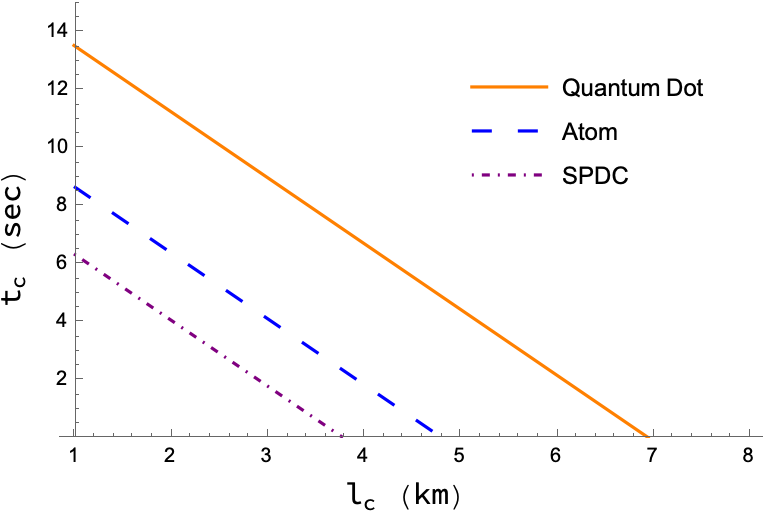
Figure 8: In this figure, we consider a repeater-based network and plot the critical storage time $t_{cr}$ as a function of critical fiber length $l_{cr}$ for different qubit architectures. The single photon architectures have efficiencies (a) $\eta_{s}$ = 0.97 (Quantum Dots Press et al. (2007)) (b) $\eta_{s}=0.88$ (Atoms Barros et al. (2009)) and (c) $\eta_{s}=0.84$ (SPDC Altepeter et al. (2005)). We set $p_{\ast}=0.5$, $q=1$, $\alpha=1/22\text{ km}^{-1}$ and $\beta=1/50\text{ sec}^{-1}$. (Color online)

Let us introduce a finite number of repeater stations between the two end nodes, each performing Bell measurements on its share of qubits. The network is useful for $\mathrm{Task}_{\ast}$ when

$$q^{r}~{}\eta_{s}^{r+1}~{}\mathrm{e}^{-2r(\alpha l+\beta t)}>p_{\ast},$$ (26)

where $r$ denotes the number of repeater stations between the end nodes. Let $l_{cr}$ and $t_{cr}$ denote the critical length of the fiber and the critical storage time of the quantum memory. These two critical parameters are then related via the expression

$$\alpha~{}l_{cr}+\beta~{}t_{cr}<\frac{1}{2r}\ln\bigg(\frac{q^{r}\eta_{s}^{r+1}}{p_{\ast}}\bigg{missing}).$$ (27)

We plot in Fig. 9 the critical fiber length $l_{cr}$ and the critical storage time $t_{cr}$ such that Eq. (27) holds for different values of $r$. The bounds on $l_{cr}$ and $t_{cr}$ for other values of $r$ not shown in Fig. 9 can be obtained from Eq. (27). We observe that for a given information processing task, increasing the number of repeater stations allows shorter fiber lengths and quantum memory storage times.

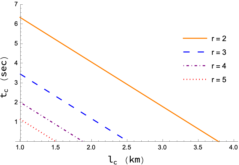
Figure 9: In this figure, we consider a repeater-based network and plot the critical storage time $t_{cr}$ as a function of critical fiber length $l_{cr}$ for the different numbers of repeater stations. We set $p_{\ast}=0.5$, $\alpha=1/22\text{ km}^{-1}$, $\beta=1/50\text{ sec}^{-1}$, $q=1$ and $\eta=0.999$. (Color online)

We note that the optimal rate of two-way assisted quantum communication or entanglement transmission (i.e., in an informal way, it is the maximum number of ebits per use of the channel in the asymptotic limit of the number of uses of the channel) over an erasure channel, also called LOCC (local operations and classical communication)-assisted quantum capacity of an erasure channel, is given by $\eta_{e}\log_{2}d$ Bennett et al. (1997), where $1-\eta_{e}$ is the erasing probability and $d$ is the dimension of the input Hilbert space. Two-way assisted quantum and private capacities for erasure channel coincide Goodenough et al. (2016); Pirandola et al. (2017) (see Wilde et al. (2017) for strong-converse capacity). Two-way assisted private and quantum capacities for a qubit erasure channel is $\eta_{e}$ Goodenough et al. (2016); Pirandola et al. (2017).

In the following section, we present limitations on the scalability of networks for quantum communication tasks assuming some hypothetical scheme can improve the transmittance of quantum channels connecting the nodes of the network.

IV.3 Limitations on quantum network topologies

Let us consider an equilateral triangle-mesh network having the set of nodes as $\mathbb{V}$ (see Fig. 10(a) for $n=3$). The nodes of the triangle network are connected by qubit erasure channels having transmittance $\eta=\mathrm{e}^{-(\alpha l+\beta t)}$, where $l$ denotes the distance between the nodes and $t$ is the time it takes for some resource $\chi$ to pass through the channel.

Let us introduce a repeater scheme in the form of a star network (see Fig. 10(b) for $n=3$) to effectively mitigate the losses due to transmission. The star network has virtual channels connecting the repeater node $v_{R}$ to the node $v_{i}\in\mathbb{V}$. The transmittance of the virtual channels $\eta_{R}=\eta^{1/\sqrt{3}}$ is greater than $\eta$.

We now consider the transmittance of channels connecting pairs of nodes with a hypothetical scheme in a network that would lead to the following assumption.

Assumption 1.

Let us assume there exist repeater-based quantum communication or quantum key distribution schemes that can mitigate the loss due to transmittance of a quantum channel such that the rate of communication (ebits or private bits per channel use Das et al. (2021)) is effectively of the order

$$\eta_{R}=\eta^{1/f}$$ (28)

in some regime (distance), where $\eta$ is the transmittance of the channel and for some $f\geq 1$ (cf. Lucamarini et al. (2018); Wang et al. (2018); Ma et al. (2018); Zeng et al. (2020)).

To illustrate Assumption 1, let us consider a regular polygon network with $n$ nodes having vertex set $\mathbb{V}$ and edge set $\mathbb{E}$ as shown in Fig. 10(a). For $e_{ij}\in\mathbb{E}$ the nodes $\{v_{i},v_{j}\}$ are connected by erasure channels having transmittance $\eta=\mathrm{e}^{-\alpha l}$, where $l$ is the distance between the nodes. Let us introduce a repeater scheme in the form of a star network as shown in Fig. 10(b) having the vertex set $\mathbb{V}_{s}\coloneqq\mathbb{V}\cup\{v_{R}\}$ where $v_{R}$ denotes the repeater node and the edge set is denoted by $\mathbb{E}_{s}$. For $e_{kR}\in\mathbb{E}_{s}$ the channel connecting nodes $\{v_{k},v_{R}\}\in\mathbb{V}_{s}$ have transmittance $\eta_{R}=\mathrm{e}^{-\alpha l/2\sin(\pi/n)}$, where $n=|\mathbb{V}|$. Comparing with Eq. (28) we observe that the star network provides an advantage of $f=2\sin(\pi/n)$ over a repeater-less scheme for $n<6$. For the triangle network discussed previously, we have $f=\sqrt{3}$. There may be other repeater-based schemes which uses entanglement distillation and error-correction techniques to further mitigate the transmission loss and enhance the rate of communication between end nodes.

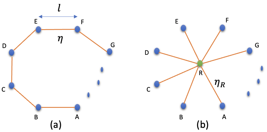
Figure 10: In this figure, we show (a) repeater-less regular polygon network with $n$ nodes and (b) star-repeater network with $n$ nodes. (Color online)

In Eq. (28), the case of $f=1$ has been shown in  Das et al. (2021) for measurement-device-independent quantum key distribution (see Pirandola et al. (2017); Wilde et al. (2017) for quantum key distribution over point-to-point channel) and the case of $f=2$ has been shown in Lucamarini et al. (2018); Wang et al. (2018); Ma et al. (2018); Zeng et al. (2020); Xie et al. (2023) for twin-field quantum key distribution and asynchronous measurement-device-independent quantum key distribution Xie et al. (2022); Zhou et al. (2023). In Fig. 11, we set $\beta=0$ and plot the variation of $\eta_{R}$ as a function of the channel length $l$ for different values of $f$.

Consider the task of sending ebits or private bits over the qubit erasure channel at a rate greater than $p_{\ast}$. To successfully perform the task, the critical length $l_{c}$ and the critical time $t_{c}$ are related via the expression

$$\alpha l_{c}+\beta t_{c}\leq-f\ln p_{\ast}.$$ (29)

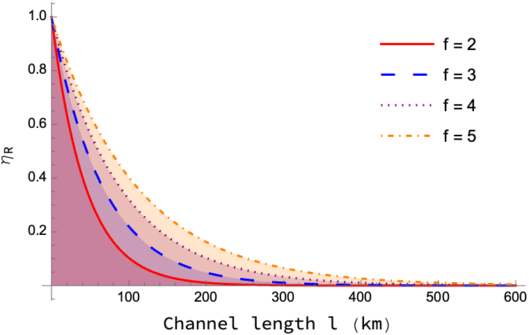
Figure 11: In this figure, we plot the variation of $\eta_{R}$ as a function of the channel length $l$ (km) (setting $\beta=0$) for different values of $f$. (Color online)

We see from Eq. (29) that using repeaters provides $f-$fold advantage over repeater-less networks. We plot in Fig. 12 the critical length $l_{c}$ and critical time $t_{c}$ for sending ebits or private bits over the channel at a rate $p_{\ast}=0.5$ for different values of $f$. In the plot, we have set $\alpha=1/22$ km^-1, and $\beta=1/10$ s^-1.

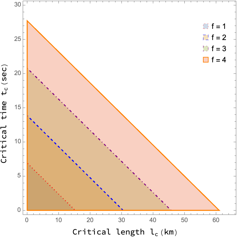
Figure 12: In this figure, we plot the critical length $l_{c}$ (km) and critical time $t_{c}$ (sec) for sending ebits or private bits over the channel at a rate of $p_{\ast}=0.5$ for different values of $f$. We have considered $\alpha=1/22$ km^-1 and $\beta=1/10$ sec^-1. (Color online)

We next consider performing quantum communication over a lattice network with fiber-based elementary links and present limitations on its scalability.

Observation 2.

Let us require to perform $\mathrm{Task}_{\ast}$ over the lattice $G_{lat}(\mathbb{V},\mathbb{E})$ having open edges with probability $p_{ij}$ and $0<p_{\ast}\leq p_{ij}<1$. It follows from Theorem 1 that for any vertex $v\in\mathbb{V}$, the set of vertices connected to it via a network path is finite. This implies $G_{lat}$ has a finite diameter. We may assume the elementary link formed by edge $e_{ij}\in\mathbb{E}$ connecting nodes $\{v_{i},v_{j}\}\in\mathbb{V}$ to be optical fibers of length $L$ having attenuation factor of $\alpha_{dB/km}=0.22$ dB/km. The fibers having transmittance $\eta=\mathrm{e}^{-\alpha L}$ where $\alpha=0.051$/km. Let there be some repeater-based scheme that increases the transmittance from $\eta$ to $\eta^{1/f}$ (see Assumption 1). Assuming that performing $\mathrm{Task}_{\ast}$ by the nodes $\{v_{i},v_{j}\}$ requires transmittance of at least $\epsilon(=0.5)$ bounds the length of the fiber to $L\leq(f/\alpha)\ln(1/\epsilon)\approx 27$ km for $f=2$. If there are $r=10$ elementary links each of length $L=27$ km between two nodes separated by a distance $l=rL=270$ km, then performing $\mathrm{Task}_{\ast}$ requires $f\geq rL\alpha/\ln(1/\epsilon)\approx 20$.

In the following example, we present limitations on the scalability of DI-QKD networks assuming there exists some scheme that can mitigate loss due to transmittance over a quantum channel.

Example 1.

Let us consider the task of connecting end nodes separated by the continental scale of (order of $1000$ km) distance. To enable such a task, let there be a repeater-based network with $t=10$ elementary links connecting two virtual nodes separated by metropolitan distances (order of $100$ km). Each elementary link has two sources say $S_{i}$ and $S_{j}$ producing dual-rail encoded entangled pairs (for details see Appendix A) in the state $\Psi^{+}$. The sources $S_{i}$ and $S_{j}$ send one qubit from its entangled pair to the nearest virtual node and the other to the repeater station via optical fibers of length $l=25$ km having attenuation factor $\alpha=0.04$ km^-1. Let the qubits evolve through the fiber as a qubit erasure channel (see Sec. E.2) with channel parameter $\eta_{e}=\mathrm{e}^{-(\alpha l/f)}$, where we assume that some technique allow us to increase the transmissivity of optical fiber by factor $1/f$ for $f>1$. After passing through the optical fiber, the qubits are stored in identical quantum memories at the repeater station, the virtual nodes, and the end nodes for $n=2$ time steps. We model the evolution of the qubits in the quantum memory as depolarising channel (see Sec. E.1) having channel parameter $p=0.01$. Assuming the repeater station performs ideal Bell measurement on its share of qubits, the singlet fidelity of the state shared by Alice and Bob is given by $\eta_{0.01}^{2}~{}\mathrm{e}^{-2\alpha lt/f}$. The state shared by the end nodes is useful for CHSH-based DI-QKD protocols if $\eta_{0.01}^{2}~{}\mathrm{e}^{-2\alpha lt/f}\geq 0.7445$ which requires $f\geq 37$.

Observation 2 and Example 1 illustrate how far is current technology from designing quantum networks for performing quantum communication and implementing DI-QKD protocols.

In the analysis of networks represented as graphs, it is important to analyze the robustness of the network for different information-processing tasks. In recent works, the robustness has been studied in the context of removal of network nodes Albert et al. (2000) and has been modelled as a percolation process on networks Callaway et al. (2000); Das et al. (2018a); Mohseni-Kabir et al. (2021) represented as graphs. In these studies, the vertices are considered present if the nodes connecting them are functioning normally. In the following subsection, taking motivations from degree centrality Freeman et al. (1979), betweenness centrality Freeman (1977) and Gini index Gini (1912) of network graphs we present figures of merit to compare the robustness of network topologies. We then compare different network topologies based on these measures.

IV.4 Robustness measure for networks

Networks that have a large number of edges are more tolerant to non-functioning nodes and edges as compared to those with fewer edges. Taking motivation from the degree centrality of a graph Freeman et al. (1979), we define the link sparsity of a network to assess the performance of a network.

Definition 7.

Consider a network $\mathscr{N}(G(\mathbb{V},\mathbb{E}))$ having the effective success matrix as $\mathbb{f_{\ast}}.$ Let the total number of entries and the number of non-zero entries in $\mathbb{f_{\ast}}$ be $m$ and $m_{\ast}$ respectively. The link sparsity of such a network is given by

$$\Upsilon(\mathscr{N})=1-\frac{m_{\ast}}{m}.$$ (30)

Typically it is desirable for the network to have low values of link sparsity. The networks represented as graphs can exist in different topologies and have the same number of nodes, edges and also the same weighted edge connectivity. These networks are said to be isomorphic to one another.

Definition 8.

(Graph isomorphism West (2000)) The graphs $G(\mathbb{V},\mathbb{E},\mathbb{L})$ and $G^{\prime}(\mathbb{V^{\prime}},\mathbb{E^{\prime}},\mathbb{L}^{\prime})$ are isomorphic iff there exists a bijective function $f:\mathbb{V}\to{\mathbb{V^{\prime}}}$ such that:

• $\forall u\in\mathbb{V},l\in\mathbb{L},l^{\prime}\in\mathbb{L}^{\prime},~{}l(u)=l^{\prime}(f(u))$

• $\forall u,v\in\mathbb{V},~{}(u,v)\in\mathbb{E}\leftrightarrow(f(u),f(v))\in\mathbb{E^{\prime}}$

• $\forall(u,v)\in\mathbb{E},l\in\mathbb{L},l^{\prime}\in\mathbb{L}^{\prime},~{}l(u,v)=l^{\prime}(f(u),f(v))$

It follows from Eq. (30) that isomorphic networks have the same value of link sparsity. Networks having the same value of link sparsity can differ in the distribution of edge weights. Taking motivation from the betweenness centrality of a graph Freeman (1977), we define the connection strength of the nodes in the network and the total connection strength of the network.

Definition 9.

Consider a network $\mathscr{N}(G(\mathbb{V},\mathbb{E}))$ with $|\mathbb{V}|=N_{v}$ having the adjacency matrix and the effective success matrix as $\mathbf{A_{\ast}}$ and $\mathbb{f_{\ast}}.$ The connection strength of a node $v_{i}$ in the network $\mathscr{N}$ is given by

$$\zeta_{i}(\mathscr{N})\coloneqq\begin{cases}\bigg{(}\sum_{\begin{subarray}{c}j\\ j\neq i\end{subarray}}2^{-[\mathbf{A}_{\ast}]_{ij}}\bigg{)}/N_{v}&\text{non-cooperative},\\ \bigg{(}\sum_{\begin{subarray}{c}j\\ j\neq i\end{subarray}}[\mathbb{f}_{\ast}]_{ij}\bigg{)}/N_{v}&\text{cooperative}.\end{cases}$$ (31)

The total connection strength of the network $\mathscr{N}$ in the (non-)cooperative strategy is obtained by adding the connection strengths of the individual nodes and is given by

$$\Gamma(\mathscr{N})=\sum_{j}\zeta_{j}(\mathscr{N}).$$ (32)

In the following subsection, we compare the robustness measures for different network topologies.

IV.5 Comparison of the robustness of network topologies

The topology of a network is defined as the arrangement of nodes and edges in the network. The information processing task that the network is performing decides the topology of the network. Two of the most commonly used network topologies are the star and mesh topologies.

A star network topology Stallings (1984) of $n$ nodes is a level 1 tree with 1 root node and $n-1$ leaf nodes. A star network with $8$ nodes is shown in Fig. 13. The root node labelled $1$ is the hub node and acts as a junction connecting the different leaf nodes labelled $2$ to $8$.

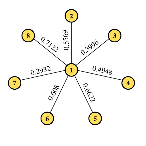
Figure 13: In this figure, we present a star network with $8$ nodes. The node $v_{1}$ is the hub and nodes $v_{2}$ to $v_{8}$ are the outer nodes. The functioning of the hub node is critical to the functioning of the network. (Color online)

Among all network topologies, this network typically requires the minimum number of hops for connecting two nodes that do not share an edge between them. The working of the hub is most critical to the functioning of the star network. The failure of a leaf node or an edge connecting a leaf node to the root does not affect the rest of the network. As an example of its use, this type of network finds application as a router or a switch connecting a ground station to different locations in an entanglement distribution protocol. In such a protocol, an adversary can attack the root node to prevent the proper functioning of the network. If the root node fails to operate, all leaf nodes connected to it become disconnected.

In a mesh network topology Green (1980), each node in the network shares an edge with one or more nodes, as can be seen from Fig. 14(a) and 14(b). There are two types of mesh topologies depending on the number of edges connected to each node. A mesh is called fully connected if each node shares an edge with every other node of the network, as shown in Fig. 14(a). A mesh is called partially connected if it is not fully connected, as shown in Fig. 14(b). A mesh where each node shares an edge with only one other node of the network is called a linear network.

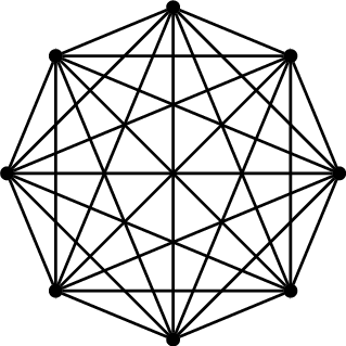
(a) Fully connected mesh with 8 nodes

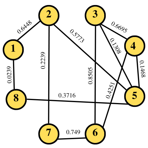
(b) A partially connected mesh with 8 nodes.

Figure 14: In this figure, we present (a) fully connected and (b) partially connected mesh networks with $8$ nodes. In a fully connected mesh network, there are edges between every pair of nodes. The presence of multiple paths between two nodes of the mesh network makes it more robust as compared to a star network with the same number of nodes. (Color online)

In a partially or fully connected mesh, the presence of multiple paths between two nodes of the network makes it robust. As an example of its use, a mesh network can be used for a satellite-based entanglement distribution, which we discuss in detail in a later section.

Let us consider a mesh network $\mathscr{N}_{m}(G_{m}(\mathbb{V},\mathbb{E}))$ of diameter $d$ with $|\mathbb{V}|=N_{v}$ and for $(v_{i},v_{j})\in\mathbb{E},$ $p_{ij}=p.$ Let there be a non-cooperating strategy for sharing resources between the nodes of the network. For such a strategy, the rows of the adjacency matrix of the network have $N_{z}$ number of zero entries where $0\leq N_{z}\leq N_{v}-1.$ Next, let there also exist a cooperating strategy for sharing resources between the nodes of this network. For such a strategy, the node $v_{i}$ of the network does not share an edge with $N^{\prime}_{z}$ number of nodes where $0\leq N^{\prime}_{z}\leq N_{z}\leq N_{v}-1.$ From the remaining nodes, there exists edges between $v_{i}$ and $(N_{v}-N^{\prime}_{z}-1)/d$ number of nodes with $p_{ij}=p^{j}$ where $1\leq j\leq d.$ For such a network, we have the link sparsity as

$$\Upsilon(\mathscr{N}_{m})\coloneqq\begin{cases}(N_{z}+1)/N_{v}&\text{non-cooperating,}\\ (N^{\prime}_{z}+1)/N_{v}&\text{cooperating.}\end{cases}$$ (33)

The connection strength of the node $v_{i}$ is given by

$$\zeta_{i}(\mathscr{N}_{m})\coloneqq\begin{cases}\big{[}1+p(N_{v}-N_{z})\big{]}/N_{v}&\text{non-cooperating,}\\ \big{[}1+\frac{p(p^{d}-1)(N_{v}-N^{\prime}_{z}-1)}{d(p-1)}\big{]}/N_{v}&\text{cooperating.}\end{cases}$$ (34)

The total connection strength of the network is given by $\Gamma(\mathscr{N}_{m})=N_{v}\times\zeta_{i}(\mathscr{N}_{m})$. It can be seen that for this network the sparsity index $\Xi(\mathscr{N}_{m})$ (see Eq. (68)) is the same as the connection strength of the node. This follows from the equal distribution of the weights in the network.

Next consider a star network $\mathscr{N}_{s}(G_{s}(\mathbb{V},\mathbb{E}))$ with $|\mathbb{V}|=N_{v}$ and for $(v_{i},v_{j})\in\mathbb{E}$ we have

$$p_{ij}\coloneqq\begin{cases}p&\text{if $i=1$ and $p\geq p_{\ast}$},\\ 0&\text{otherwise}.\end{cases}$$ (35)

The link sparsity of such a network is $\Upsilon(\mathscr{N}_{s})=1-(1/N_{v})$ for the cooperative strategy and $\Upsilon(\mathscr{N}_{s})=1-[(3N_{v}-2)/N_{v}^{2}]$ for the non-cooperative strategy. The connection strength of the root node is $\zeta_{i}(\mathscr{N}_{s})=(1+p(N_{v}-1))/N_{v},$ while for the leaf nodes is

$$\zeta_{i}(\mathscr{N}_{s})\coloneqq\begin{cases}(1+p)/N_{v}&\text{non-cooperative},\\ [1+p+p^{2}(N_{v}-2)]/N_{v}&\text{cooperative.}\end{cases}$$ (36)

The sparsity index (see Eq. (68)) of the network is

$$\Xi(\mathscr{N}_{s})\coloneqq\begin{cases}\big{[}N_{v}^{2}+p(N_{v}^{2}\\ \qquad\qquad\quad+N_{V}-2)\big{]}/N_{v}^{3}&\text{non-cooperative},\\ \big{[}N_{v}^{2}+p(N_{v}-1)(N_{v}+2)\\ \qquad+p^{2}(N_{v}-2)(N_{v}-1)\\ \qquad\qquad(N_{v}+1)\big{]}/N_{v}^{3}&\text{cooperative.}\end{cases}$$ (37)

As another example, consider a network $\mathscr{N}(G(\mathbb{V},\mathbb{E}))$ having $|V|=N_{v}$ number of nodes, and each node shares an edge with $d$ other nodes. The effective adjacency matrix $\mathbf{A}_{\ast}$ of such a network is a circulant matrix. Let the success probability of transferring a resource between the node $1$ and the node $n$ be given by,

$$p_{1n}\coloneqq\begin{cases}p^{n}&\text{if $n\leq d/2$ and d = even},\\ p^{d-n+1}&\text{if $n>d/2$ and d = even},\\ p^{n}&\text{if $n\leq(d+1)/2$ and d = odd},\\ p^{d-n+1}&\text{if $n>(d+1)/2$ and d = odd}.\end{cases}$$ (38)

The first row of the adjacency matrix is formed by calculating the weights $w_{\ast}(e_{1n})=-\log p_{1n}.$ The $k^{\text{th}}$ row is formed by taking the cyclic permutation of the first row with an offset equal to $k.$ In the non-cooperative strategy, the link sparsity of the network is then given by

$$\Upsilon(\mathscr{N})=1-\bigg{(}\frac{d+1}{N_{v}}\bigg{)},$$ (39)

and the connection strength of the node $v_{i}$ is given by

$$\zeta_{i}(\mathscr{N})\coloneqq\begin{cases}\frac{(1+p)(p^{(d+1)/2}-1)}{N_{v}(p-1)}&\text{if $d$ is odd},\\ \frac{1}{N_{v}}\bigg{[}1+\frac{2p(p^{d/2}-1)}{(p-1)}\bigg{]}&\text{if $d$ is even}.\end{cases}$$ (40)

In the following subsection, we introduce measures for identifying the critical nodes of a given network.

IV.6 Critical nodes in a network

The critical nodes of a network are the nodes that are vital for the proper functioning of the network. Removing any of these nodes can lead to some of the other nodes in the network being disconnected. Given a network $\mathscr{N}(G)$, we proceed to define a measure for the criticality of the nodes in $G$. For this, at first, taking motivation from Watts and Strogatz (1998), we define the clustering coefficient for the nodes of a given network.

Definition 10.

For a network $\mathscr{N}(G)$, let $G_{i}(\mathbb{V}_{i},\mathbb{E}_{i})$ be a sub-graph of $G$ formed by the neighbours of node $v_{i}\in\mathbb{V}.$ Let $n_{i}=|\mathbb{V}_{i}|$ be the number of nodes present in $G_{i}$ and $e_{i}=|\mathbb{E}_{i}|$ be the number of edges present in $G_{i}$ with $p_{ij}\geq p_{\ast}$. The clustering coefficient of the node $v_{i}$ is defined as

$$C_{i}=\frac{2~{}e_{i}}{n_{i}(n_{i}-1)}.$$ (41)

The average clustering coefficient of a network is calculated by taking the average of $C_{i}$ for all the nodes of the network. We next proceed to define the average effective weight of a network using Eq. (15).

Definition 11.

For a network $\mathscr{N}(G)$, the average effective weight of a network denoted by $\widetilde{\mathrm{w}}_{\ast}$ is defined as the mean of the effective weight between all the node pairs in the network and is expressed as

$$\widetilde{\mathrm{w}}_{\ast}(G)=\frac{1}{n(n-1)}\sum_{\begin{subarray}{c}v_{i},v_{j}\in\mathbb{V}\\ i\neq j\end{subarray}}\mathrm{w}_{\ast}({e_{i\to{...}\to{j}}}),$$ (42)

where $\mathrm{w}_{\ast}({e_{i\to{...}\to{j}}})$ is the effective weight associated with the path connecting the nodes $v_{i}$ and $v_{j}$.

When two nodes $(v_{i},v_{j})$ are disconnected, the effective weight $\mathrm{w}_{\ast}({e_{i\to{...}\to{j}}})$ becomes infinite. Small values of $\widetilde{\mathrm{w}}_{\ast}(G)$ indicate that the network performs the task with high efficiency.

Definition 12.

For a network $\mathscr{N}(G)$, let us denote the shortest path connecting the node pairs $(v_{i},v_{j})\in G$ as $d_{ij}\in\mathbb{D}$. We define the centrality $\tau_{i}$ of the node $v_{i}$ as the number of paths belonging to the set $\mathbb{D}$ in which the node $v_{i}$ appears as a virtual node. The critical parameter associated with the node $v_{i}$ is defined as

$$\nu=\frac{\tau_{i}}{C_{i}\widetilde{w}_{\ast}(G_{i})}.$$ (43)

The critical nodes of a graph have high values of $\nu$. These nodes of the network are essential for the proper functioning of the network. If one of these nodes is removed, it will lead to a decrease in the overall efficiency of the network. Quantum network architectures have potential applications in diverse fields ranging from communication to computing. In the following section, we present the bottlenecks of some potential use of quantum networks for real-world applications.

V Real World Instances

In this section, we first present practical bottlenecks in the distribution of entangled pairs between two far-off cities. We then consider different currently available as well as near-future quantum processor architectures as networks and observe their robustness parameters. Then we propose networks for (a) the major international airports to communicate via a global quantum network and (b) the Department of Energy (DoE) at Washington D.C. to communicate with the major labs involved in the National Quantum Initiative (NQI) by sharing entanglement. We present the practical bottlenecks for such models.

V.1 Entanglement distribution between cities

Consider a satellite-based network for sharing entangled pairs between two far-off cities. Let such a network be a two-layered model consisting of a global scale and a local scale. On a global scale, there are multiple ground stations located across different cities. Such ground stations are interconnected via a satellite network. Two ground stations share an entangled state using the network via the shortest network path between them (see Sec. VI.1 for details of the shortest path algorithm.)

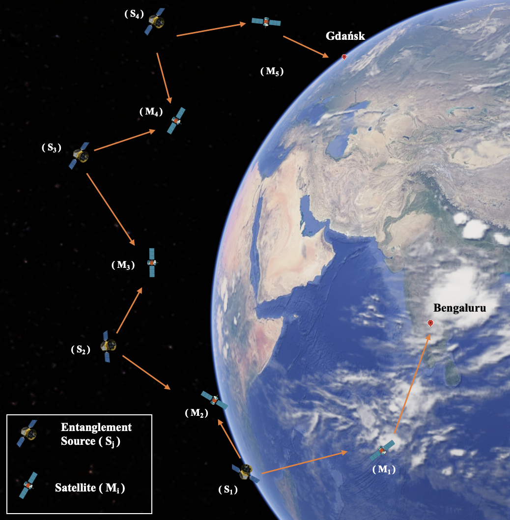
Figure 15: In this figure, we present the shortest network path between the ground stations at Bengaluru and Gdańsk via the global satellite network. The entangled sources are marked as $S_{i}$ and the satellite stations are marked as $M_{i}$. The shortest path has $6$ entangled sources and $5$ satellite stations. The image was created using the Google Earth software Google ([Online]). (Color online)

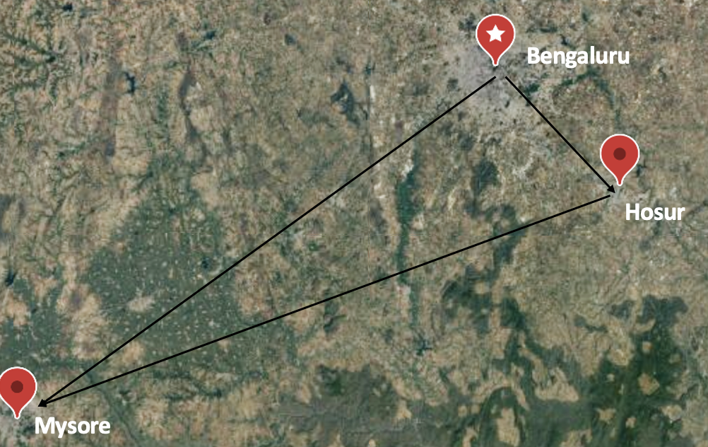
(a) Bengaluru ground station

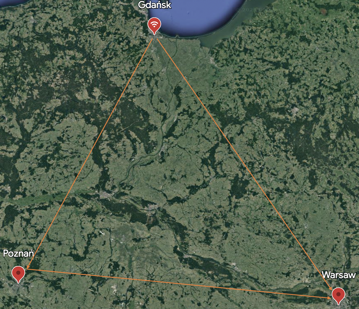
(b) Gdańsk ground station

Figure 16: In this figure, we present the local scale network architectures at (a) Bengaluru and (b) Gdańsk for sharing entangled pairs across nearby localities. The ground stations are connected to multiple localities via optical fibers (shown in black and orange lines). The images were created using Google Earth software Google ([Online]). (Color online)

As an example, we show in Fig. 15 the shortest path connecting the ISTRAC ground station located at Bengaluru to the ground station at Gdańsk via the global satellite network. On the local scale, different localities (end nodes) are connected to their nearest ground station via optical fibers. We show in Fig. 16 the local scale network for the ground station located at Bengaluru and Gdańsk. The ground station at Bengaluru is connected to the localities of Hosur and Mysore. The ground station at Gdańsk is connected to the localities of Poznań and Warsaw.

In the satellite network, there are sources $(S_{j})$ producing entangled photonic qubit pairs in the state $\Psi^{+}$. The source then sends the photons belonging to a pair to different neighbouring satellites via a quantum channel as shown in Fig. 15. We model the quantum channel between the ground station and the satellite at the limits of the atmosphere as a qubit thermal channel (see Sec. E.3 and Sec. F) and that between two satellites as an erasure channel (see Sec. E.2) having erasure parameter $\eta_{e}$. The erasure channel parameter is assumed to be identical throughout the network. The satellite stations $M_{j}$ outside the limits of the atmosphere perform Bell measurement on their share of the qubits that they received from their neighbouring source stations. The satellites at the boundary of the atmosphere transmit their share of qubit via the atmospheric channel to the ground stations (which we call local servers). The ground stations on receiving the state store it in a quantum memory. In the quantum memory, the state evolves via a depolarising channel (see Sec. E.1). The local servers distribute the quantum states to different localities (which we call clients) on request using optical fibers as can be seen in Fig. 16.

In future, it may be that India and Poland establish communication links that share each halves of the entangled pairs between a designated hub in each country so that they can perform desired quantum tasks in collaboration. Let us assume that the Indian Space Research Organization (ISRO) headquarter at Bengaluru would like to perform delegated quantum computing Childs (2001); Giovannetti et al. (2008); Broadbent et al. (2009); Fitzsimons (2017); Barz et al. (2012) by securely accessing the IBM Quantum Hub at Poznań Maciag-Kruszewska and ibmblogs . For this, the ISRO headquarter can share entangled system with the IBM Quantum Hub via the shortest route in the satellite-based network. For an illustration, let the shortest network path between the ground stations at Bengaluru and Gdańsk have $5$ satellites and $4$ entangled photon sources as shown in Fig. 15. The entanglement yield of the network is given by

$$\xi_{\text{avg}}=\eta_{t}^{G}(\eta_{e}^{2})^{4},$$ (44)

where $\eta_{t}^{G}$ is obtained from Eq. (86) and takes into account the local weather conditions at Bengaluru and Gdańsk. In the general network with $n$ satellite-to-satellite links between the two ground stations, the average entanglement yield is given by

$$\xi_{\text{avg}}=\eta_{t}^{G}(\eta_{e}^{2})^{n}.$$ (45)

The ground stations store the incoming qubits in different quantum memory slots and serve the receiving traffic requests from different local clients following queuing discipline (see Sec. VI.4). The total number of memory slots available in the quantum memory is fixed. The evolution of the stored qubits in the quantum memory is modelled via a depolarising channel with channel parameter $p$. We model the quantum memory as a max-heap data structure (see Definition 3) with the key as the fidelity of the stored quantum state. If the fidelity of any quantum state stored in the memory drops below a pre-defined critical value, $\eta_{\text{crit}}$, that state is deleted from the memory. The value of $\eta_{\text{crit}}$ is determined by the task or the protocol that the end parties may be interested in performing using their shared entangled state. On receiving a connection request from a single local client, the ground station transmits the latest qubit that it has received as outward traffic. Now when the ground station receives traffic requests from multiple local clients, there is the problem of optimizing the traffic flow. For such a flow problem, we introduce the following modified fair queuing algorithm.

Let us define $t_{p}^{(i)}$ as the time to process the $i^{\text{th}}$ quantum state in the memory, $t_{i}^{(i)}$ as the starting time for the transmission from the memory and $t_{f}^{(i)}$ as the time when the state has been transmitted from the memory. We then have,

$$t_{f}^{(i)}=t_{i}^{(i)}+t_{p}^{(i)}.$$ (46)

Now, there is a possibility that the state has arrived at the memory before or after the processing of $i-1$ states in this heap. In the latter case, the state arrives at an empty heap memory and is transmitted immediately if there is a traffic request. In the other case, it swims through the heap depending on its fidelity and is stored in the memory. Let us denote $t_{r}^{(i)}$ as the time required for the node to swim up to the root node from its current position in the heap. Then we have,

$$t_{f}^{(i)}=\max\bigg{(}t_{f}^{(i-1)},t_{r}^{(i)}\bigg{)}+t_{p}^{(i)},$$ (47)

where $t_{f}^{(i-1)}$ is the time required for processing $(i-1)^{\text{th}}$ quantum state. If there are multiple flows, the clock advances by one tick when all the active flows receive one state following the qubit-by-qubit round-robin basis. If the quantum state has spent $s$ time steps in the memory then the average entanglement yield is given by

$$\xi_{\text{avg}}\coloneqq\begin{cases}\eta_{d}^{s}\hskip 3.0pt\eta_{t}^{G}(\eta_{e}^{2})^{n}&\text{if }\eta_{d}^{s}>\eta_{\text{crit}},\\ 0&\text{otherwise,}\end{cases}$$ (48)

where $\eta_{d}$ is obtained from Eq. (74) and takes into account the loss in yield per time step in the quantum memory. Let us assume the ground station at Bengaluru and Gdańsk transmits the state via identical fibers to the ISRO headquarter and Poznań, respectively. Considering the fiber losses at the two ground stations given by $\mathrm{e}^{-\alpha l_{B}}$ and $\mathrm{e}^{-\alpha l_{M}}$, the sources producing the state $\Psi^{+}$ with probability $\eta_{s}$, and assuming that the quantum state has spent $s$ time steps in the memory, the average entanglement yield is given by

$$\xi_{\text{avg}}=\eta_{d}^{s}\hskip 3.0pt\eta_{t}^{G}(\eta_{e}^{2})^{n}(\eta_{s})^{n-1}\mathrm{e}^{-\alpha(l_{B}+l_{M})},$$ (49)

where $l_{B}$ and $l_{M}$ are the lengths of the fibers from ISRO headquarter and Poznań to the Bengaluru and Gdańsk ground stations respectively. Inserting $\eta_{t}^{G}$ from Eq. (86), we have the yield given by

$$\xi_{\text{avg}} =\mathrm{e}^{-\alpha(l_{B}+l_{M})}\left(\eta_{e}^{2}\right)^{n}\eta_{s}^{n-1}$$ (50)

$$\bigg{[}(1-p)^{2s}-\frac{1}{4}(p-2)p\left((s-1)(1-p)^{2(s-1)}+1\right)\bigg{]}$$

$$\qquad\qquad\bigg{[}(n_{1}-1)n_{1}(\eta_{1}-1)^{2}+\frac{1}{2}(1+\eta_{1}^{2})\bigg{]}$$

where $\eta_{1}$, $n_{1}$ take into account the local weather condition at Bengaluru and Gdańsk and $s$ is the number of applications of depolarising channel in the quantum memory.

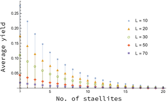
Figure 17: In this figure, we plot the average yield $\xi_{\text{avg}}$ (see Eq. (50)) as a function of the number of satellites in the network for different values of the total optical fiber length $L=l_{B}+l_{M}$ (shown figure inset). We set $\eta_{s}=0.9,s=1,p=0.1,\eta_{e}=0.95,\eta_{1}=0.5,n_{1}=0.5,\alpha=1/22$ km^-1. (Color online)

We plot in Fig. 17, the average entanglement yield $\xi_{\text{avg}}$ of the two end nodes connected by the network as a function of the number of satellite-to-satellite links $n$ between their nearest ground stations for different values of the total optical fiber length $L=(l_{B}+l_{M})$. We observe that for a fixed value of $L$, $\xi_{\text{avg}}$ decreases with an increase in $n$. Also, for a fixed value of $n$, $\xi_{\text{avg}}$ decreases with increase in $L$.

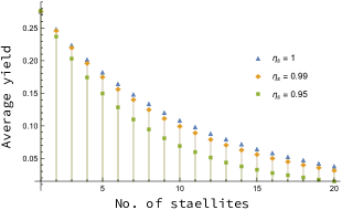
Figure 18: In this figure, we plot the average yield $\xi_{\text{avg}}$ (see Eq. (50)) as a function of the number of satellites in the network for single photon source architectures. The single photon source architectures have the source efficiencies (a) $\eta_{s}=0.95$ (b) $\eta_{s}=0.99$ and (b) $\eta_{s}=1.$ For this, we set $L=l_{B}+l_{M}=10$ km$,s=1,p=0.95,\eta_{e}=0.95,\eta_{1}=0.5,n_{1}=0.5,\alpha=1/22$ km^-1. (Color online)

Furthermore, we plot in Fig. 18 and 30 the variation in $\xi_{\text{avg}}$ as a function of $n$ for different values of $\eta_{s}$. We observe that for a given $\eta_{s}$, $\xi_{\text{avg}}$ decreases with increase in $n$. Also, we observe that Quantum dot-based, atom-based, and SPDC-based entangled photon sources are best suited for the entanglement distribution network.

Our methods in general apply to sharing multipartite entangled states among different ground stations distributed at different geographical locations across the globe. To observe this, note that if certain users of the network share bipartite entangled states, then such states can be used to distill multipartite entangled states with the use of ancilla and entanglement swapping protocols Zeilinger et al. (1997); de Bone et al. (2020); Das et al. (2021).

V.2 Quantum Processors

The currently available quantum processors (QPUs) use different technologies to implement the physical processor. The processors of IonQ and Honeywell utilize a trapped ion-based architecture, while IBM, Rigetti, and Google have a superconducting architecture. The superconducting architecture requires physical links between qubits that are to be entangled, while the trapped ion-based architecture does not have any topological constraint. In this section, we model the different quantum processor architectures as graphical networks (see Table 1) and present the robustness measures (defined in Sec. IV.4) for such networks.

Name	Layout	Fidelity	Qubits	$T_{1}$
Sycamore (Google) AI (2021)	square lattice	$96.9\%$ (RO) $99.85\%$ (1Q) $99.64\%$ (2Q)	54	15 $\mu s$
Eagle (IBM) (2022) (2022); Begušić et al. (2023)	heavy hexagonal	$99.96\%$ (RO) $99.99\%$ (1Q) $99.94\%$ (2Q)	127	95.57 $\mu s$
Aspen-M-2 (Rigetti) Computing (2020)	octagonal	$97.7\%$ (RO) $99.8\%$ (1Q) $90\%$ (2Q)	80	30.9 $\mu s$

Table 1: The performance details of different quantum processors. In the above table, the second column provides the arrangement of the qubits in the processor. The third column provides the 1 qubit (1Q), 2 qubits (2Q), and the readout (RO) fidelity of the processors. The fourth column provides the total number of qubits in the processor, and the fifth column provides the thermal relaxation time $(T_{1})$ of the qubits of the processor.

We consider different qubit quantum processor network architectures in square, heavy-hexagonal and octagonal layouts. The link sparsities of each unit cell for these different network layouts are given by

$$\Upsilon\mathscr{(}{N})\coloneqq\begin{cases}1-\big{(}\frac{16}{64}\big{)}\approx 0.75&\text{octagonal,}\\ 1-\big{(}\frac{8}{16}\big{)}\approx 0.5&\text{square,}\\ 1-\big{(}\frac{24}{144}\big{)}\approx 0.833&\text{heavy hexagonal.}\end{cases}$$ (51)

We observe that the square structure has the lowest link sparsity, followed by octagonal and heavy hexagonal structures. Next, let the edges present in these network layouts have success probability $p$.

The connection strength of the $i^{th}$ node in the unit cell of octagonal, heavy hexagonal and square network for a non-cooperative strategy is given by

$$\Gamma(\mathscr{N})\coloneqq\begin{cases}p/4&\text{octagonal,}\\ p/2&\text{square,}\\ p/6&\text{heavy hexagonal.}\end{cases}$$ (52)

We plot in Fig. 1 the connection strength of the $i^{th}$ node for different values of the success probability of edge. We observe that the connection strength for a given success probability of edge is highest for square networks, followed by octagonal and heavy-hexagonal networks.

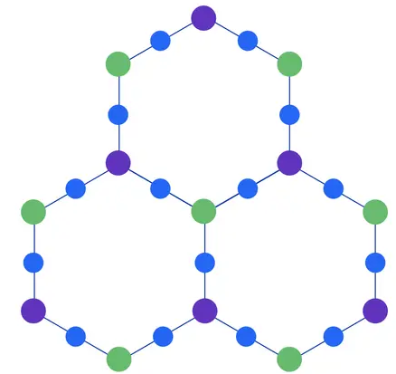
Figure 19: A slice of a quantum processor model based on heavy-hexagonal structure discussed in Nation et al. (2021). The link sparsity of the unit cells in the network is $0.833$, and the critical nodes of the network slice are shown in green and violet. (Color online)

We propose a 1024-node square lattice-based quantum processor network architecture represented as a $32\times 32$ lattice.

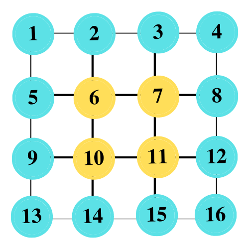
Figure 20: A $4\times 4$ slice of a $1024$ node quantum processor architecture based on square structure. The total network layout is represented as a $32\times 32$ lattice. The link sparsity of the network is $0.9962$, and the critical nodes of the network slice are shown in yellow. (Color online)

We show in Fig. 20 a $4\times 4$ slice of the lattice as a representation of the entire quantum processor. The link sparsity of the $1024$ node square network is $0.9962$. The nodes shown in yellow in Fig. 20 are identified as critical nodes. We observe in Fig. 20 that there are three types of nodes in the network based on the number of edges that are connected to the node. We call a node a corner node, edge node, and inner node if it shares an edge with two, three, and four other nodes, respectively. The connection strength of these three types of nodes is given by

$$\zeta_{i}(\mathscr{N})\coloneqq\begin{cases}p/256&\text{inner node,}\\ 3p/1024&\text{boundary node,}\\ p/512&\text{corner node.}\end{cases}$$ (53)

V.3 Network propositions

Let us first consider a network connecting all the major airports in the world. We say that two airports are connected if there exists at least one commercial airline currently operating between them. We consider a network consisting of 3463 airports all over the globe forming the nodes of the network and 25482 edges or airline routes between these airports Lawrence ([Online]). For such a network, we observe that the longest route is between Singapore, Changi International Airport, and New York John F. Kennedy International Airport, in the United States, with a distance of approximately 15331 km. The average distance between the airports in the network is approximately 1952 km. We propose a quantum network with airports as nodes and the connections between the airports as edges. We define the edge weight of the edge connecting the nodes $\{v_{i},v_{j}\}$ of the network as

$$\mathrm{w}(e_{ij})\coloneqq\begin{cases}\mathrm{e}^{-L_{ij}/22}&\text{if $L_{ij}<50$ km}\\ 0.8&\text{if $L_{ij}\geq 50$ km}\end{cases}$$ (54)

where $L_{ij}$ is the distance between two airports denoted by nodes $v_{i}$ and $v_{j}$. The link sparsity of such a network is 0.99575, and the total connection strength is given by 0.99787. We observe that the most critical airports present in this network are Istanbul International Airport, Dubai International Airport, Anchorage Ted Stevens in Alaska, Beijing Capital International Airport, Chicago O’Hare International Airport, and Los Angeles International Airport.

Let the airports of the network require to securely communicate with each other. The sharing of entangled states among the airports is a primitive for secure communication among them. Let us assume all these airports are located at the same altitude. Let the ground stations located at the airports share an entangled state using a global satellite-based mesh quantum network as described in Sec. V.1. The ground stations connect to the satellite network via the atmospheric channel modelled as a qubit thermal channel. The satellites of the network are interconnected via a qubit erasure channel. For two airports $a_{1}$ and $a_{2}$ requiring to connect, the average entanglement yield is given by

$$\xi_{\text{avg}} =\eta_{t}^{a}(\eta_{e}^{2})^{n}$$

$$=\left(\eta_{e}^{2}\right)^{\left\lfloor\frac{L}{L_{0}}\right\rfloor}\bigg{[}(n_{1}-1)n_{1}(\eta_{1}-1)^{2}+\frac{1}{2}(1+\eta_{1}^{2})\bigg{]},$$

where $L$ denotes the distance between $a_{1}$ and $a_{2}$. $L_{0}$ denotes the distance between the nodes of the satellite network. We assume identical atmospheric conditions at $a_{1}$ and $a_{2}$ and set $\eta_{e}=0.95,\eta_{1}=0.5$ and $n_{1}=0.5.$ With these choices of parameters, we present in Fig. 21 the average yield as a function of the distance between the nodes of the satellite network for different values of $L$. The entanglement yield between the airports for different channel parameters not considered in this section can be obtained from Eq. (LABEL:eq:yieldAirportNetwork).

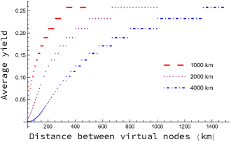
Figure 21: In this figure, we plot the average yield $\xi_{\text{avg}}$ (see Eq. (LABEL:eq:yieldAirportNetwork)) as a function of the distance between the virtual nodes for different lengths between the airports. For this, we set $\eta_{e}=0.95,\eta_{1}=0.5,n_{21}=0.5$. (Color online)

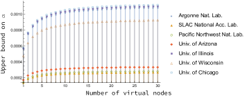
Figure 22: The upper bound on the channel parameter $\alpha$ for sharing entanglement between the U.S. Department of Energy (DoE) at Washington D.C. and some other labs Office of Science involved in The National Quantum Initiative (NQI). In this network, the DoE is the hub node while the labs are at the outer nodes. The edge connecting the hub to an outer node represents a repeater relay network. (Color online)

The quantum Internet can be used for secure communication between a central agency and end parties. It may be desirable here for the central agency to prevent direct communication between the end parties. As an example, consider the U.S. Department of Energy (DoE) in Washington D.C. require to securely communicate by sharing entangled states with the major labs Office of Science that are involved in The National Quantum Initiative (NQI) using the Star network. The DoE is at the hub node of such a network and the different labs are the leaf nodes. For each edge of the network, let there be independent fiber-based repeater chain networks (described in Sec. III.) Let each edge present in the network have a success probability $p=\mathrm{e}^{-\alpha L/n}$ where $\alpha$ is the channel loss parameter, $L$ is the total distance between the DoE and the lab, and $n$ is the number of virtual nodes. Using Eq. (95), we obtain the upper bound on $\alpha$ as

$$\alpha<\frac{\log(3)}{L(1+\frac{1}{n})}.$$ (56)

For different labs, we plot in Fig. 22 the upper bound on $\alpha$ for different values of $n$. In the figure, we have considered some of the major labs, which can be extended to all other labs involved in the NQI.

In the following section, we present graph algorithms that are primitives for implementing different information-processing tasks using the quantum Internet.

VI Algorithms

In Sec. VI.1, we provide an algorithm to find the shortest path between a pair of end nodes. We then provide an algorithm in Sec. VI.2 to constrict a network architecture for sharing resources between n two parties, each having multiple nodes. In Sec. VI.3, we provide an algorithm to identify the critical nodes of a given network. Then in Sec. VI.4, we provide an algorithm to optimize the flow of resources at a node having multiple input and output channels.

VI.1 Shortest path between a pair of nodes

For performing $\mathrm{Task}_{\ast}$ with maximum success probability, it is desirable to transmit resource $\chi$ between any two nodes via the shortest network path connecting them. Recent works have considered different network topologies Schoute et al. (2016); Chakraborty et al. (2019); Li et al. (2020) and limitations on current and near-term hardware Khatri (2021, 2022b); Iñesta et al. (2023) for routing resources over quantum networks. For a given network $\mathscr{N}$ represented as a graph $G$, we consider here the task of finding the path between two given nodes in $G$ that have the lowest effective weight for routing resources between them Schoute et al. (2016). We call a path connecting two nodes in the network and having the lowest effective weight as the shortest path between them. Finding the shortest path between two nodes of a network is important as longer paths are more vulnerable to node and edge failures. To find the shortest path between two nodes, we introduce a modified version of Dijkstra’s algorithm Dijkstra (1959) in Algorithm 1. In Algorithm 1, the shortest spanning tree is generated with the source node as the root node. Then the nodes in the tree are stored in one set and the other set stores the nodes that are not yet included in the tree. In every step of the algorithm, a node is obtained that is not included in the second set defined above and has a minimum distance from the source.

Algorithm 1 Modified Dijkstra’s algorithm

1:function dijkstra($G,S,\text{target}$)

2:     Initialize:

3:      $\text{pq}\leftarrow\text{empty min priority queue}$ $\text{dist}\leftarrow\varnothing$ $\text{pred}\leftarrow\varnothing$

4:     for every node in G do

5:         if node $=S$ then

6:              pq[node] $\leftarrow$ 0

7:         else

8:              pq[node] $\leftarrow$ infinite               

9:     for every node and minDist in pq do

10:         dist[node] $\leftarrow$ minDist

11:         if node = target then

12:              break          

13:         for every neigh of node do

14:              if neigh $\in$ pq then

15:                  score $\leftarrow$ dist[node] + $G[\text{node, neigh}][\text{weight}]$

16:                  if score $<$ pq[neigh] then

17:                       pq[neigh] $\leftarrow$ score

18:                       pred[neigh] $\leftarrow$ node                                               return dist, pred

To obtain the shortest path between any two nodes of a given graph, we apply Algorithm 2 to implement the modified Dijkstra’s algorithm. The algorithm returns the shortest path between the source node and the end node in the graph.

Algorithm 2 Obtaining the shortest path between the source and target nodes in a graph

1:Initialize:

2:      $source\leftarrow\text{starting node}$ $\text{target}\leftarrow\text{target node}$

3:G $\leftarrow$ the given graph

4:[dist, pred] $\leftarrow$ DIJKSTRA(G, source, target)

5:end $\leftarrow$ target

6:path $\leftarrow$ [end]

7:while end $\neq$ source do

8:     end = pred[end]

9:     path.append(end)

10:disp(path)

Example 2.

Let us consider a weighted graph with $8$ nodes as shown in Fig. 23.

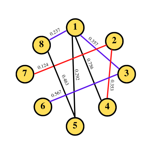
Figure 23: A network represented by a weighted graph with $8$ nodes. Multiple pairs of nodes can share resources using this network. As an example, nodes $(8,6)$ can share resource via the path $8\leftrightarrow 1\leftrightarrow 3\leftrightarrow 6$ (shown in blue), then nodes $(7,4)$ can share resource via the path $7\leftrightarrow 2\leftrightarrow 4$ (shown in red). (Color online)

A physical interpretation can be to consider the transfer of quantum states from node $v_{i}$ to node $v_{j}$ via quantum channels denoted by the edges. The edge weight between the nodes $v_{i}$ and $v_{j}$ is given by $-\log p_{ij}$ where $p_{ij}$ is the success probability of sharing the resource between these two nodes. The shortest path connecting the nodes would then provide the highest success probability for the task. If we consider the source as node $v_{8}$ and the target as node $v_{6}$, then the algorithm returns the shortest path as $v_{8}\leftrightarrow v_{1}\leftrightarrow v_{3}\leftrightarrow v_{6}.$ It may be desirable for another node say $v_{7}$ to share a resource with node $v_{4}$ using the same network. The node $v_{7}$ and $v_{4}$ can share resources via the path $v_{7}\leftrightarrow v_{2}\leftrightarrow v_{4}$ without involving the virtual nodes in the shortest path between $(v_{8},v_{6})$. We observe that multiple pairs of nodes can share resources using this network.

In the following subsection, we present an algorithm to construct a network for sharing resources between two parties each having multiple nodes.

VI.2 Network Construction

Let two parties Alice (denoted by $A$) and Bob (denoted by $B$) require to share a resource using a mesh network. We assume that $A$ and $B$ have $n_{A}$ and $n_{B}$ number of nodes respectively. We introduce Algorithm 3 to obtain the structure of the mesh that ensures there exist distinct paths between nodes of $A$ and $B$. In Algorithm 3, we impose the constraints that (a) at a time all nodes of $A$ shall be connected to distinct nodes of $B$ via the shortest available path with unique virtual nodes and (b) there exists a path between every nodes of $A$ and $B$.

Algorithm 3 Network construction algorithm

1:function network($n_{A},n_{B}$)

2:     Initialize:

3:      count $\leftarrow n_{A}+n_{B}$ g $\leftarrow$ complete graph (no. of nodes: count) g[weight] $\leftarrow$ mesh edge weights

4:     for every node $i$ of $A$ do

5:         add edge to g (i, count, weight)

6:         count $\leftarrow$ count + 1      

7:     for every node $i$ of $B$ do

8:         add edge to g (i, count, weight)

9:         count $\leftarrow$ count + 1      return g

Example 3.

Consider two geographically separated companies $A$ and $B$ requiring to connect to each other via a mesh network. We call the headquarters of the companies as hubs. In Fig. 24 we show the hubs of $A$ and $B$ in blue and orange respectively.

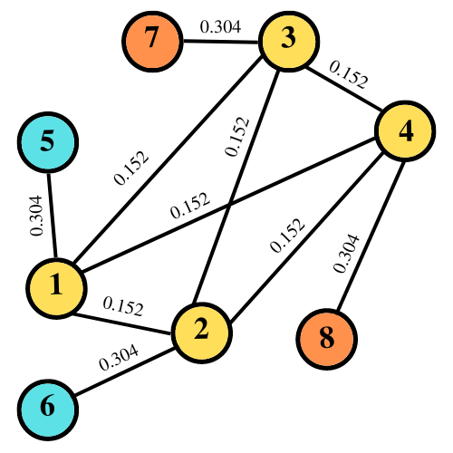
Figure 24: A $4$ node network (shown in yellow) constructed using Algorithm 3 for connecting the hubs $A$ and $B$. The hubs $A$ and $B$ each have two nodes and are shown in orange and blue respectively. (Color online)

Using Algorithm 3 we obtain the network topology for which there exists distinct paths for possible pairs of $(a_{i},b_{j})$ where $a_{i}\in A$ and $b_{j}\in B$.

In the following subsection, we consider a given network represented as a graph and present an algorithm to identify the critical nodes of the network.

VI.3 Identifying the critical nodes

The critical nodes of the network are essential for the proper functioning of the network. If one of these nodes is removed, it will lead to a decrease in the overall performance efficiency of the network. We present Algorithm 4 to obtain the critical parameter $\nu$ for the nodes of the network using Eq. (43). The nodes with the highest values of $\nu$ are identified as the critical nodes of the network. These are the nodes that are the most important for the proper functioning of the graphical network.

Algorithm 4 Finding the critical nodes in a given graph

1:G $\leftarrow$ the given graph

2:for every node in G do

3:     $C_{i}\leftarrow$ clustering coeff using Eq. (41)

4:     $\bar{\mathrm{w}}_{\ast}(G)\leftarrow$ avg cost using Eq. (42)

5:     $\tau_{i}\leftarrow$ centrality of the node

6:     $\nu_{i}\leftarrow\tau_{i}/C_{i}~{}\bar{\mathrm{w}}_{\ast}(G)$

7:critNodes $\leftarrow$ list of nodes with high values of $\nu_{i}.$

Example 4.

Let us use Algorithm 4 to obtain the critical nodes of the graph with $8$ nodes shown in Fig. 25.

Figure 25: A network represented by a weighted graph with $8$ nodes and $12$ edges. Node $v_{6}$ (shown in yellow) is the most critical node followed by nodes $v_{2}$ and $v_{5}$ (shown in orange). These nodes are the most critical for the proper functioning of the network. (Color online)

We have the critical parameter for different nodes in the network as

node number $(i)$	$\nu_{i}$	node number $(i)$	$\nu_{i}$
$v_{1}$	0.1714	$v_{5}$	1.5238
$v_{2}$	1.6667	$v_{6}$	2.5714
$v_{3}$	0.7619	$v_{7}$	0.1714
$v_{4}$	0.9523	$v_{8}$	0.5714

We observe that node $v_{6}$ is the most critical followed by node $v_{2}$ and node $v_{5}$. We label these nodes as the critical nodes of the network.

In the following subsection, we introduce an algorithm for optimizing the flow of resources at a node that has multiple input and output channels.

VI.4 Resource allocation at a node

The nodes of a network can have a buffer memory where resources such as incoming packets from different input channels can be stored and later distributed via different output channels to neighbouring nodes based on traffic request. We introduce Algorithm 5 for the optimal flow of resources at a node having multiple input and output channels.

Algorithm 5 Resource allocation at a node

Initialize:

      $\text{buffSize}\leftarrow\text{size of buffer}$ $\text{buffer}\leftarrow\varnothing$

procedure Producer(thread)

     while items produced and empty buffer slot do

         gain access to buffer

         store item at empty buffer slot

         update other memory slots as per task

         release the buffer      

procedure Consumer(thread)

     while buffer is not empty do

         gain access to buffer

         acquire item from the buffer

         update other memory slots as per task

         release the buffer      

create and start all producer threads

create and start all consumer threads

In Algorithm 5, the procedures CONSUMER threads are the instances of the output channels that extract packets from the buffer and the PRODUCER are the instances for the input channels that inputs packets to the buffer.

VII Discussion

We envision that the implementation of the quantum Internet will follow a task-oriented approach. The underlying network structure at any stage of implementation is expected to provide loose coupling, meaning end users can perform information processing tasks without requiring to know the details of implementation, thereby reducing dependencies between different tasks. This requires assessing the practical limitations for implementing different tasks.

Our work provides a step in that direction by taking a graph theory (and information theory-)based approach to analyze the scalability and robustness of the quantum Internet. Focusing on the latter part, we have provided measures for comparing the robustness and identifying the critical nodes of different network topologies. Identifying quantum processors as real-world mesh networks, we compared the robustness measures for the quantum processor architectures by Google, IBM, and Rigetti. With the vision of having a 1024-qubit quantum processor in the future, we extend the 54-qubit layout by Google to include 1024 qubits and observe the robustness of such a network.

The network structure of the quantum Internet is determined by the information processing tasks that are implemented using it. Looking at the elementary link level, we have obtained bounds on the critical success probability for performing different tasks. Extending to a more general repeater-based network, we have obtained a trade-off between the channel length and the time interval for which the states can be stored at the nodes such that the shared state is useful for different tasks.

Considering performing some desirable information processing tasks over lattice networks, we present a theorem specifying conditions that lead to the absence of percolation. As implications of the theorem, we highlight the constraints on network scalability and limitations of current technology for performing quantum communication and implementing DI-QKD protocols.

Looking at the specific details of implementation, considering repeater-based networks, we have provided the range of isotropic state visibility and an upper bound on the number of repeater nodes for distilling secret keys at non-zero rates via DI-QKD protocols. We have considered practical parameters like atmospheric conditions and imperfect devices in obtaining bottlenecks for implementing a satellite-based model distributing resources between far-off places. For such a network we have presented algorithms for implementing certain underlying network-related tasks such as obtaining the network layout, obtaining the network routing path and allocating resources at the network nodes. Overall, the assessment presented in this paper can be used in benchmarking the critical parameters involved in realizing the quantum Internet.

Appendix A Dual rail encoding of photons

In the dual rail encoding scheme Knill et al. (2001), the qubits are encoded using the optical modes of photons. The computational basis of the photonic qubit system $A$ encoded in the polarization modes $m_{1}$ and $m_{2}$ is given by

$$\ket{H}_{A}\rightarrow\ket{1,0}_{l_{1},l_{2}},~{}\ket{V}_{A}\rightarrow\ket{0,1}_{l_{1},l_{2}}.$$ (57)

A pure state $\ket{\psi}_{A}$ of the qubit system can be expressed in such a computational basis as

$$\ket{\psi}_{A} =\alpha\ket{1,0}_{l_{1},l_{2}}+\beta\ket{0,1}_{l_{1},l_{2}}$$ (59)

$$=\alpha\ket{H}_{A}+\beta\ket{V}_{A},$$

where $\alpha,\beta\in\mathbbm{C}$ and $|\alpha|^{2}+|\beta|^{2}=1.$ The bipartite entangled state $\Psi_{AB}^{+}$ is expressed as $\Psi_{AB}^{+}=\outerproduct{\Psi^{+}}{\Psi^{+}}_{AB}$ where $\ket{\Psi^{+}}_{AB}=\frac{1}{\sqrt{2}}(\ket{HH}_{AB}+\ket{VV}_{AB})$.

Appendix B Two-qubit states

The maximally entangled states for the two-qubit systems can be expressed as

$$\Phi^{\pm}_{AB}\coloneqq\outerproduct{\Phi^{\pm}}{\Phi^{\pm}}_{AB}$$

$$\Psi^{\pm}_{AB}\coloneqq\outerproduct{\Psi^{\pm}}{\Psi^{\pm}}_{AB}$$ (60)

where $\ket{\Psi}^{\pm}_{AB}$ and $\ket{\Phi}^{\pm}_{AB}$ are defined as

$$\ket{\Psi}^{\pm}_{AB}:=\frac{1}{\sqrt{2}}\bigg{(}\ket{00}_{AB}\pm\ket{11}_{AB}\bigg{)},$$ (61)

$$\ket{\Phi}^{\pm}_{AB}:=\frac{1}{\sqrt{2}}\bigg{(}\ket{01}_{AB}\pm\ket{10}_{AB}\bigg{)}.$$ (62)

Following from Eq. (3), a two-qubit isotropic state can be expressed as

$$\rho_{AB}^{I}(p,2)=\frac{1}{3}(4p-1)\Psi^{+}_{AB}+\frac{4}{3}(1-p)\frac{\mathbbm{1}_{AB}}{4}.$$ (63)

Similarly, following from Eq. (5), a two-qubit Werner state can be expressed as

$$\rho_{AB}^{W}(p(\lambda),2)=\lambda\Psi^{-}_{AB}+(1-\lambda)\frac{\mathbbm{1}_{AB}}{4},$$ (64)

where $\lambda\in[-1/3,1]$.

Appendix C Two qubit Bell measurement on isotropic states

Let there be a measurement station that performs Bell measurement on the halves of two-qubit isotropic states $\rho_{A_{1}A_{1}^{\prime}}^{I}(p^{\prime}(\lambda),2)$ and $\rho_{B_{1}B_{1}^{\prime}}^{I}(p^{\prime}(\lambda),2)$, where

$$\rho_{AB}^{I}(p^{\prime}(\lambda),2):=\lambda\Psi^{+}_{AB}+(1-\lambda)\frac{\mathbbm{1}_{AB}}{4}.$$ (65)

We call $\lambda$ the visibility of the isotropic state $\rho_{AB}^{I}(p^{\prime}(\lambda),2)$. Let the success probability of a Bell measurement be $q$. We denote the action of the noisy Bell measurement channel as

$$\mathcal{E}_{A_{1}^{\prime}B_{1}^{\prime}\to I_{A}I_{A}^{\prime}I_{B}I_{B}^{\prime}}\bigg{(}\rho_{A_{1}A_{1}^{\prime}}^{I}(p^{\prime}(\lambda),2)\otimes\rho_{B_{1}B_{1}^{\prime}}^{I}(p^{\prime}(\lambda),2)\bigg{)}$$

$$=~{} \frac{\lambda^{2}q}{4}\bigg{[}\Psi_{A_{1}B_{1}}^{-}\otimes\outerproduct{00}{00}_{I_{A}I_{B}}$$ (66)

$$+\Psi_{A_{1}B_{1}}^{+}\otimes\outerproduct{11}{11}_{I_{A}I_{B}}+\Phi_{A_{1}B_{1}}^{-}\otimes\outerproduct{22}{22}_{I_{A}I_{B}}$$

$$+\Phi_{A_{1}B_{1}}^{+}\otimes\outerproduct{33}{33}_{I_{A}I_{B}}\bigg{]}\otimes\outerproduct{00}{00}_{I_{A}^{\prime}I_{B}^{\prime}}$$

$$+(1-\lambda^{2})q\frac{\mathbbm{1}_{A_{1}B_{1}}}{4}\otimes\frac{1}{4}\sum_{i=0}^{3}\outerproduct{ii}{ii}_{I_{A}I_{B}}\otimes\outerproduct{00}{00}_{I_{A}^{\prime}I_{B}^{\prime}}$$

$$+(1-q)\frac{\mathbbm{1}_{A_{1}B_{1}}}{4}\otimes\outerproduct{\perp}{\perp}_{I_{A}I_{B}}\otimes\outerproduct{11}{11}_{I_{A}^{\prime}I_{B}^{\prime}}.$$

The flag state $\outerproduct{11}{11}_{I_{A}^{\prime}I_{B}^{\prime}}$ indicates error in the Bell measurement with a probability $(1-q)$ and the state $\frac{\mathbbm{1}_{A_{1}B_{1}}}{4}$ is left on $\mathscr{H}_{A_{1}B_{1}}$. The flag state $\outerproduct{00}{00}_{I_{A}^{\prime}I_{B}^{\prime}}$ indicates a successful Bell measurement with probability $q$. If error corrections are possible post-Bell measurement, then from a single use of repeater we have the state

$$\rho_{AB}^{W}(p(\lambda^{2}),2)=\lambda^{2}~{}\Psi^{+}_{AB}+(1-\lambda^{2})\frac{\mathbbm{1}_{AB}}{4}$$ (67)

with a probability $q$.

Appendix D Sparsity Index

Taking motivation from the Gini Index of network graphs Gini (1912) and using the definition of the connection strength of the nodes in a network, we define the sparsity index of the network.

Definition 13.

Consider the plot with the cumulative sum of the number of nodes in the network $\mathscr{N}(G(\mathbb{V},\mathbb{E}))$ along the horizontal axis and the cumulative sum of $\zeta_{i}(G)$s along the vertical axis. The sparsity index of the network $\mathscr{N}$ is given by

$$\Xi(\mathscr{N})=\frac{\text{area enclosed by the curve and x-axis}}{\text{area enclosed by the $45^{\circ}$ line}}.$$ (68)

As an example, the star network $\mathscr{N}_{s}(G_{s}(\mathbb{V},\mathbb{E}))$ (see Eq. (35)) with $N_{v}=8$ and $p=0.5$ have sparsity index $0.1934$ for non-cooperative strategy and $0.3779$ for cooperative strategy. The sparsity index $\Xi(\mathscr{N})$ of the network $\mathscr{N}$ measures the extent of inequality in the distribution of connection strength among the nodes of the network. High values of $\Xi$ indicate a high cumulative percentage of connection strength for the cumulative fractile of the nodes. Typically it is desirable for the network to have high values of sparsity index.

Appendix E Actions of some quantum channels

E.1 The qubit depolarizing channel

The action of a qubit depolarizing channel Bennett et al. (1996b) on the qubit density operator $\rho_{A}$ is given by

$$\mathcal{D}_{A\rightarrow B}(\rho_{A})=(1-p)\hskip 5.0pt\rho_{B}+p\hskip 5.0pt\frac{\mathbbm{1}_{B}}{2},$$ (69)

where $p\in[0,\frac{4}{3}]$ is the channel parameter and $\mathbbm{1}_{B}$ is the identity operator. In the formalism given by Kraus Kraus (1971) and Choi Choi (1975) the effect of the channel can be defined by the following operators Romero and Franco (2012),

$$\mathcal{K}_{0}=\sqrt{1-\frac{3p}{4}}\hskip 5.0pt\mathbbm{1}$$ (70)

and $$\mathcal{K}_{i}=\frac{\sqrt{p}}{2}\hskip 5.0pt\mathbbm{\sigma}_{i}\text{ with }i\in\{1,2,3\},$$ (71)

where $\sigma_{i}$ are the Pauli matrices. The action of the depolarizing channel on each of the systems $A$ and $\bar{A}$ is given by,

$$\mathcal{D}_{A\rightarrow B}\hskip 2.0pt\otimes\hskip 2.0pt\mathcal{D}_{\bar{A}\rightarrow\bar{B}}\left(\Psi_{A\bar{A}}^{+}\right)$$

$$=\sum_{i=0}^{4}\sum_{j=0}^{4}\left(\mathcal{K}_{i}\otimes\mathcal{K}_{j}\right)\Psi_{A\bar{A}}^{+}\left(\mathcal{K}_{i}\otimes\mathcal{K}_{j}\right)^{\dagger}$$ (72)

$$=(-1+p)^{2}~{}\Psi_{B\bar{B}}^{+}+\hskip 5.0ptp\hskip 5.0pt(2-p)\hskip 5.0pt\frac{\mathbbm{1}_{B\bar{B}}}{4}$$ (73)

Noting that $\mathbbm{1}_{B\bar{B}}$ can be expressed as the sum of four maximally entangled states, we have the fidelity of the final state to the starting state as $\eta_{d}=1-\frac{3}{4}\hskip 5.0ptp\hskip 5.0pt(2-p).$ Following the approach of Iñesta et al. (2023) and applying the depolarising channel $n$ times, the final state after the evolution through the channel is

$$\rho_{B\bar{B}}^{n}=\left(\mathcal{D}_{A\rightarrow B}\hskip 2.0pt\otimes\hskip 2.0pt\mathcal{D}_{A\rightarrow B}\right)^{\otimes n}\left(\Psi_{A\bar{A}}^{+}\right).$$

This state $\rho_{B\bar{B}}^{n}$ has a fidelity with $\Psi_{B\bar{B}}^{+}$ given by

$$\eta_{d}^{n}=(1-p)^{2n}-\frac{1}{4}(p-2)p\left((n-1)(1-p)^{2(n-1)}+1\right),$$ (74)

where it can be seen that $\eta_{d}^{1}=\eta_{d}$. We plot in Fig. 26, the variation of $\eta_{d}^{n}$ (using Eq. (74)) as a function of the number of applications $n$ of the depolarising channel and the depolarising channel parameter $p$.

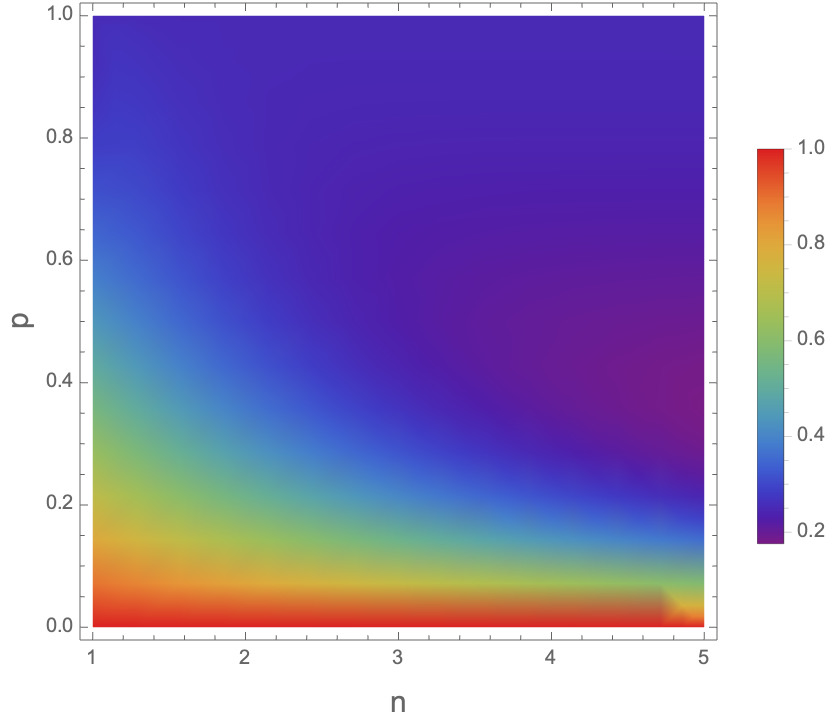
Figure 26: In this figure, we plot the variation of $\eta_{d}^{n}$ as a function of $n$ and $p$. (Color online)

E.2 The erasure channel

The action of a qubit erasure channel Grassl et al. (1997) on an input density operator $\rho_{A}$ is given by

$$\mathcal{E}_{A\rightarrow B}(\rho_{A})=\eta_{e}\rho_{B}+(1-\eta_{e})\operatorname{Tr}[\rho_{B}]\outerproduct{e}{e}_{B}.$$ (75)

The action of the erasure channel on the qubit system is such that it outputs the exact input state with probability $\eta$ or with probability $1-\eta$ replaces it with erasure state $\ket{e}$, where $\ket{e}$ is the vacuum state. The action of the channel on the maximally entangled state $\Psi_{A\bar{A}}^{+}$ in the two-qubit space $A\bar{A}$ is given by

$$\mathcal{E}_{A\rightarrow B}\hskip 5.0pt\otimes\hskip 5.0pt \mathcal{E}_{\bar{A}\rightarrow\bar{B}}\hskip 5.0pt(\Psi_{A\bar{A}}^{+})$$ (76)

$$=\eta_{e}^{2}\Psi_{B\bar{B}}^{+}+(1-\eta_{e}^{2})\Psi_{B\bar{B}}^{\perp},$$

where

$$\Psi_{B\bar{B}}^{\perp}\coloneqq\frac{\eta_{e}}{1+\eta_{e}}\bigg{(}\frac{1}{2}\mathbbm{1}_{B}\otimes\outerproduct{e}{e}_{\bar{B}}+\outerproduct{e}{e}_{B}\otimes\frac{1}{2}\mathbbm{1}_{\bar{B}}\bigg{)}$$

$$\qquad\qquad\qquad\qquad+\frac{1-\eta_{e}}{1+\eta_{e}}\outerproduct{e}{e}_{B}\otimes\outerproduct{e}{e}_{\bar{B}}$$ (77)

is a state orthogonal to $\Psi_{B\bar{B}}^{+}$.

Consider two sources creating pairs of entangled state $\Psi^{+}$. The first and second source distributes the entangled pairs to node pairs $(v_{1},v_{2})$ and $(v_{2},v_{3})$ respectively via erasure channels. The node $v_{2}$ then performs a Bell measurement on its share of states. Assuming error correction is possible post-measurement, the node pair $(v_{1},v_{3})$ share the state $\Psi^{+}$ with probability $\eta_{e}^{2}.$

E.3 The qubit thermal channel

The action of a qubit thermal channel on the density operator $\rho_{A}$ is given by

$$\mathcal{L}^{\eta_{g},n_{g}}_{A\rightarrow B}(\rho_{A})=\operatorname{Tr}_{E}[U_{\eta_{g}}\hskip 5.0pt(\rho_{A}\otimes\rho_{E})\hskip 5.0ptU_{\eta_{g}}^{\dagger}],$$ (78)

where $\rho_{E}$ is the density operator of the environment given by

$$\rho_{E}=(1-n_{g})\ket{0}\bra{0}_{E}+n_{g}\ket{1}\bra{1}_{E}.$$ (79)

The qubit thermal channel is modelled by the interaction of a qubit system $\rho_{A}$ with the environment $\rho_{E}$ at a lossy beamsplitter having transmittance $\eta_{g}$ (see Eq. (91)). The evolution through the beamsplitter is via the unitary $U_{\eta_{g}}$ expressed as

$$U_{\eta_{g}}=\left(\begin{array}[]{cccc}1&0&0&0\\ 0&\sqrt{\eta_{g}}&\sqrt{1-\eta_{g}}&0\\ 0&-\sqrt{1-\eta_{g}}&\sqrt{\eta_{g}}&0\\ 0&0&0&1\\ \end{array}\right).$$ (80)

The Generalised Amplitude Damping Channel (GADC) is equivalent to the qubit thermal channel up to the reparameterization $\mathcal{A}^{\eta_{g},n_{g}}_{A\rightarrow B}(\rho_{A})\equiv\mathcal{L}^{1-\eta_{g},n_{g}}_{A\rightarrow B}(\rho_{A})$ with $\eta_{g}\in[0,1]$ and $n_{g}\in[0,1].$ The effect of the thermal channel can be defined by the following Kraus operators in the standard basis

$$\widetilde{\mathcal{A}_{1}}=\sqrt{1-n_{g}}(\ket{0}\bra{0}+\sqrt{\eta_{g}}\ket{1}\bra{1})$$ (81)

$$\widetilde{\mathcal{A}_{2}}=\sqrt{(1-\eta_{g})(1-n_{g})}\ket{0}\bra{1}$$ (82)

$$\widetilde{\mathcal{A}_{3}}=\sqrt{n_{g}}(\sqrt{\eta_{g}}\ket{0}\bra{0}+\ket{1}\bra{1})$$ (83)

$$\widetilde{\mathcal{A}_{4}}=\sqrt{n_{g}(1-\eta_{g})}\ket{1}\bra{0}.$$ (84)

The action of the thermal channel on each of the systems $A$ and $\bar{A}$ is given by,

$$\mathcal{\tau}_{B\bar{B}}^{\eta_{g},n_{g}}\hskip 5.0pt :=\mathcal{L}^{\eta_{g},n_{g}}_{A\rightarrow B}\hskip 2.0pt\otimes\hskip 2.0pt\mathcal{L}^{\eta_{g},n_{g}}_{\bar{A}\rightarrow\bar{B}}\left(\Psi^{+}_{A\bar{A}}\right)$$

$$=\sum_{i=0}^{4}\sum_{j=0}^{4}\left(\widetilde{\mathcal{A}_{i}}\otimes\widetilde{\mathcal{A}_{j}}\right)\left(\Psi^{+}_{A\bar{A}}\right)\left(\widetilde{\mathcal{A}_{i}}\otimes\widetilde{\mathcal{A}_{j}}\right)^{\dagger}$$

$$=\eta_{g}~{}\Psi^{+}_{B\bar{B}}$$

$$\hskip 10.0pt+\hskip 5.0pt(1-\eta_{g})(n_{g}-1)\bigg{(}n_{g}(1-\eta_{g})-1\bigg{)}\ket{00}\bra{00}_{B\bar{B}}$$

$$\hskip 10.0pt+\hskip 5.0ptn_{g}(-1+\eta_{g})\bigg{(}n_{g}(-1+\eta_{g})-\eta_{g}\bigg{)}\ket{11}\bra{11}_{B\bar{B}}$$

$$\hskip 10.0pt+\hskip 5.0ptn_{g}(1-n_{g})(1-\eta_{g})^{2}\left(\ket{01}\bra{01}_{B\bar{B}}+\ket{10}\bra{10}_{B\bar{B}}\right).$$

The state $\mathcal{\tau}_{B\bar{B}}^{\eta_{g},n_{g}}$ has a fidelity with $\Psi^{+}_{B\bar{B}}$ given by

$$\eta_{t}=\frac{1}{2}(1+\eta_{g}^{2})+n_{g}(n_{g}-1)(1-\eta_{g})^{2}.$$ (86)

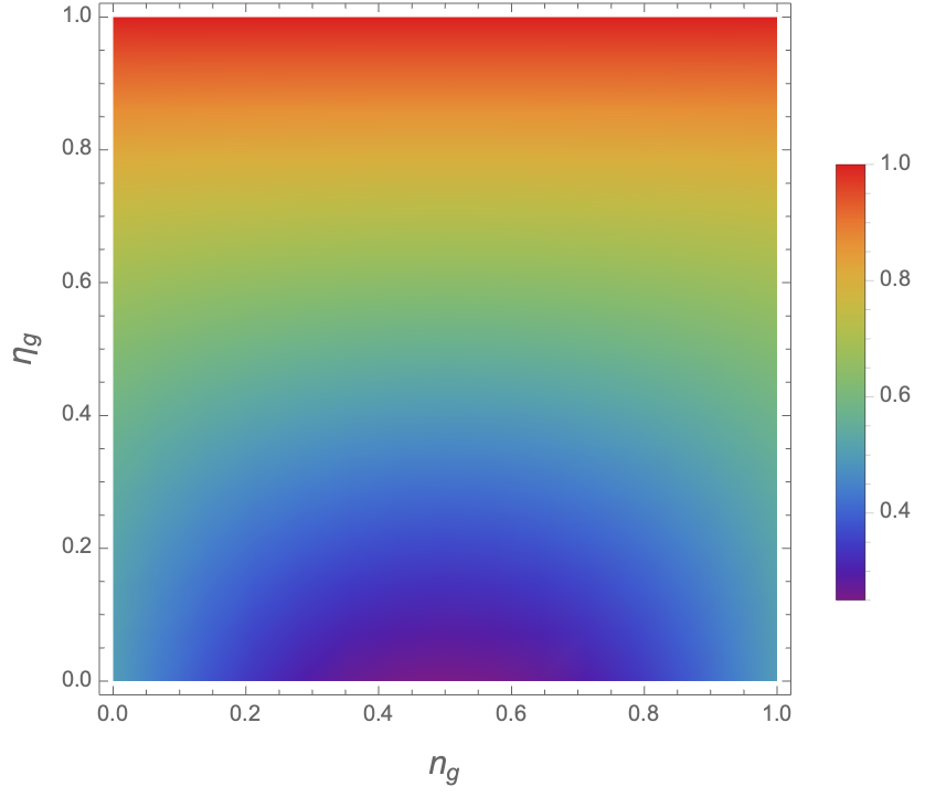
Figure 27: In this figure, we plot the variation of $\eta_{t}$ as a function of $n_{g}$ and $\eta_{g}$. (Color online)

We plot in Fig 27, the variation of $\eta_{t}$ as a function of the channel parameters $\eta_{g}$ and $n_{g}$.

Appendix F The atmospheric channel

The losses in the transmission of optical signals via an optical fiber are greater than that for free space transmission. In the vacuum space above the earth’s atmosphere, the losses are nearly negligible. The non-birefringent nature of the atmosphere causes negligible change to the polarization state of the photons passing through it. These observations motivate the use of space and satellite technologies in establishing an entanglement distribution network using such channels Lu et al. (2022). We observe in Fig. 28, that the losses in the satellite-based free-space channel is much less compared to fiber-based channels for distances greater than $~{}70\text{ km.}$

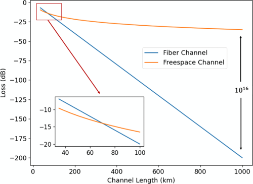
Figure 28: The comparison of losses in fiber and free-space channels as a function of channel length as discussed and plotted in Lu et al. (2022). It is observed that the free-space channel is advantageous for distances over 70 km. (Color online)

The network architecture should be a hybrid satellite-optical fiber based model with ground-based global nodes at different geographical locations that are connected to different local nodes at small distances via optical fibers. These global nodes will be connected to the inter-satellite network. This architecture can in principle be extended to deep space allowing the possibility of sharing entanglement between nodes on Earth and the moon.

The factors affecting the transmission of optical signals between a satellite and a ground station are analyzed next. We obtain the efficiency in transmission $\xi_{\text{eff}}$ considering losses due to (a) inefficiencies in transmitting $(\xi_{t})$ and receiving systems $(\xi_{r})$, (b) beam diffraction $(\xi_{d})$, (c) air turbulence $(\xi_{at})$, (d) mispointing $(\xi_{p})$ and (e) atmospheric absorption $(\xi_{as})$. The total transmittance is given by

$$\xi_{\text{eff}}=\xi_{t}\hskip 3.0pt\xi_{r}\hskip 3.0pt\xi_{d}\hskip 3.0pt\xi_{at}\hskip 3.0pt\xi_{p}\hskip 3.0pt\xi_{as}\hskip 3.0pt.$$ (87)

The diffraction of an optical beam depends on the beam’s spatial mode, wavelength and aperture of the telescope. Assuming a Gaussian beam from the source with a waist radius of $\omega_{0}$, the radius at a distance $z$ is given by $\omega_{d}(z)=\omega_{0}\sqrt{1+(z/z_{R})^{2}}$ with $z_{R}$ being the Rayleigh range. If the aperture radius of the telescope is $r$, then the receiving efficiency is given by Lu et al. (2022)

$$\xi_{d}=1-\exp{-\frac{2r^{2}}{\omega_{d}^{2}}}.$$ (88)

The turbulence in the atmosphere induces inhomogeneity in the refractive index which changes the direction of the propagating beam. It was shown in Vasylyev et al. (2016) that large-scale turbulence causes beam deflection while small-scale turbulence induces beam broadening. At the receiver end, it was shown in Dios et al. (2004) that the average long-term accumulation of the moving spots shows a Gaussian distribution with an equivalent spot radius of $\omega_{\text{at}}(z)=\omega_{d}(z)\sqrt{1+1.33\sigma_{R}^{2}\Lambda^{5/6}},$ where $\sigma_{R}^{2}$ is the Rytov variance for plane wave and $\Lambda$ is the Fresnel ratio of the beam at the receiver. The receiving efficiency is given by

$$\xi_{at}=1-\exp{-\frac{2r^{2}}{\omega_{\text{at}}^{2}}}.$$ (89)

Next, for the satellite moving at a high speed a high-precision and high-bandwidth acquisition, pointing and tracking (APT) system generally consisting of coarse and fine tracking systems is required. A combination of closed-loop coarse tracking having a large field of view along with fine tracking having a small field of view is generally used. The pointing error induces a spot jitter with the instantaneous spot following a Rice intensity distribution. It was shown in Toyoshima and Araki (1998) that the pointing efficiency is given by

$$\xi_{p}=1-\frac{\omega_{\text{at}}^{2}}{\omega_{\text{at}}^{2}+4\hskip 3.0pt\sigma_{p}^{2}},$$ (90)

where $\sigma_{p}$ is the variance of the Gaussian pointing probability distribution.

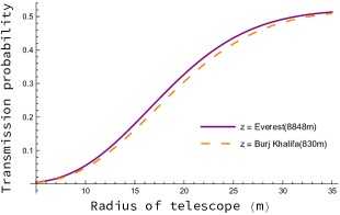
Figure 29: In this figure, we plot the variation of the transmission probability as a function of the radius of the telescope for different receiving station altitudes. For this, we have considered a $780$ nm source with $\omega_{0}=0.0021$ and quality factor $1$. We have set $z_{R}=17.8,\sigma_{R}=0.1,\Lambda=0.1,\xi_{r}=0.99,\xi_{t}=0.99,\xi_{as}=0.5$ and $\eta=0.95$. (Color online)

Inserting Eq. (88), Eq. (89), and Eq. (90) in Eq. (87) and imposing the condition that $\sigma_{p}=\eta\omega_{at}$ we obtain

$$\xi_{\text{eff}}=\frac{\eta^{2}\xi_{as}\xi_{r}\xi_{t}}{\eta^{2}+0.25}\bigg{(}1-\exp{-\frac{2r^{2}z_{R}^{2}}{w^{2}(z^{2}+z_{R}^{2})}}\bigg{)}$$

$$\left(1-\exp{-\frac{2r^{2}}{w^{2}(1.33\Lambda^{5/6}\sigma_{R}^{2}+1)(\frac{z^{2}}{z_{R}^{2}}+1)}}\right)$$ (91)

Consider a 780 nm source with a beam waist radius $\omega_{0}$ of 0.0021 m and quality factor 1. The source has a Rayleigh length $(z_{R})=17.8$ m. Let the channel have Rytov variance $(\sigma_{R})=0.1,$ and the Fresnel ratio of the beam at the receiver end is $(\Lambda)=0.1.$ Let the efficiency of the receiving unit be $(\xi_{r})=0.99,$ that of the transmitting source be $(\xi_{t})=0.99.$ Also let the probability of successful transmission after atmospheric absorption be $(\xi_{as})=0.5$. Assuming $\eta=0.95,$ we plot in Fig. 29 the transmission probability through the atmosphere as a function of the radius of the receiving telescope for different altitudes.

Appendix G Entanglement distribution across cities

We plot in Fig. 30 the variation of $\xi_{\text{avg}}$ as a function of the number of satellites in the network for different currently available single photon sources.

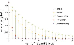
Figure 30: In this figure, we plot the average yield $\xi_{\text{avg}}$ (see Eq. (50)) as a function of the number of satellites in the network for different single photon source architectures. The single photon source architectures have the source efficiencies (a) $\eta_{s}=0.84$ (SPDC Altepeter et al. (2005)) (b) $\eta_{s}=0.88$ (Atoms Barros et al. (2009)) (c) $\eta_{s}=0.97$ (Quantum Dots Press et al. (2007)) (d) $\eta_{s}=0.35$ (NV Center Andersen et al. (2017)) and (e) $\eta_{s}=0.26$ (4 wave mixing Smith et al. (2009)). For this, we set $L=l_{B}+l_{M}=10$ km$,s=1,p=0.1,\eta_{e}=0.95,\eta_{1}=0.5,n_{1}=0.5,\alpha=1/22$ km^-1. (Color online)

Appendix H Limitations of linear repeater networks

Let us consider two distant parties, Alice and Bob requiring to share an entangled state using an entanglement swapping protocol as described in Sec. III. Assuming that there are $n$ repeater stations between Alice and Bob, they share the isotropic state

$$\rho_{AB}^{I}(p(\lambda^{n+1}),2)=\lambda^{n+1}~{}\Psi^{+}_{AB}+\frac{1}{4}(1-\lambda^{n+1})\mathbbm{1}_{AB}$$ (92)

of visibility $\lambda^{n+1}$ with a probability $q^{n}$. In the following propositions, we present the bound on the number of virtual nodes in the network such that the state $\rho_{AB}^{I}(p(\lambda^{n+1}),2)$ (a) is useful for teleportation, (b) can violate the Bell-CHSH inequality and (c) is entangled.

Proposition 3.

The state $\rho_{AB}^{I}(p(\lambda^{n+1}),2)$ can be used to perform teleportation protocol with a success probability $q^{n}$ when

$$n<\lfloor\frac{\log(3)}{\log(1/\lambda)}-1\rfloor.$$ (93)

Proof.

Let us have $u_{k}$ as the eigenvalues of the matrix $T^{\dagger}T$ where the $T$ matrix is formed by the elements $t_{nm}=\operatorname{Tr}[\rho_{AB}^{I}(p(\lambda^{n+1}),2)\hskip 3.0pt\sigma_{n}\otimes\sigma_{m}]$ where $\sigma_{j}$ denotes the Pauli matrices. We then define the quantity $N(\rho_{AB})=\sum_{k=1}^{3}\sqrt{u_{k}}$. The state $\rho_{AB}^{I}(p(\lambda^{n+1}),2)$ is useful for teleportation for values of $N(\rho_{AB})$ greater than $1$ Horodecki et al. (1996). This then implies $n<\lfloor\frac{\log(3)}{\log(1/\lambda)}-1\rfloor.$ ∎

We plot in Fig. 31 the maximum number of repeater stations that can be allowed for a given value of $\lambda$ and setting $q=0.625$ Bayerbach et al. (2022) to successfully implement a teleportation protocol.

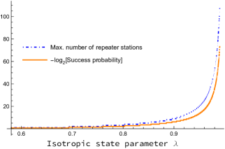
Figure 31: In this figure, we plot (a) the maximum allowed number of relay stations between Alice and Bob (shown in blue) and (b) $\log$(success probability) (in yellow) for the state $\rho^{I}_{AB}(p(\lambda^{n+1}),2)$ to be useful for teleportation protocol. (Color online)

Proposition 4.

The state $\rho_{AB}^{I}(p(\lambda^{n+1}),2)$ can violate the Bell-CHSH inequality with a success probability $q^{n}$ when

$$n<\lfloor\frac{\log(2)}{2\log(1/\lambda)}-1\rfloor.$$ (94)

Proof.

Let us have $u_{i},u_{j}$ be the two largest eigenvalues of the matrix $T^{\dagger}T$ where the $T$ matrix is formed by the elements $t_{nm}=\operatorname{Tr}[\rho_{AB}^{I}(p(\lambda^{n+1}),2)\hskip 3.0pt\sigma_{n}\otimes\sigma_{m}]$ where $\sigma_{j}$ denotes the Pauli matrices. We then define the quantity $M(\rho_{AB})=u_{i}+u_{j}$. The state $\rho_{AB}^{I}(p(\lambda^{n+1}),2)$ is Bell-CHSH nonlocal for values of $M(\rho_{AB})$ greater than $1$ Horodecki et al. (1995). This then implies $n<\lfloor\frac{\log(2)}{2\log(1/\lambda)}-1\rfloor$. ∎

We plot in Fig. 32 the maximum number of repeater stations that can be allowed for a given value of $\lambda$ and setting $q=0.625$ Bayerbach et al. (2022) such that the state shared by the end nodes can violate the Bell-CHSH inequality.

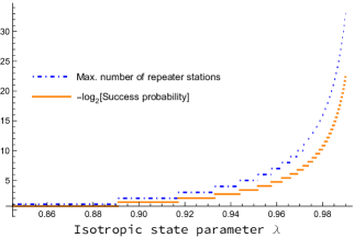
Figure 32: In this figure, we plot (a) the maximum allowed number of relay stations between Alice and Bob (shown in blue) and (b) $\log$(success probability) (in yellow) for the state $\rho^{I}_{AB}(p(\lambda^{n+1}),2)$ to violate the Bell-CHSH inequality. (Color online)

Proposition 5.

The state $\rho_{AB}^{I}(p(\lambda^{n+1}),2)$ remains entangled with a success probability $q^{n}$ when

$$n<\lfloor\frac{\log{\color[rgb]{0,0,1}(3)}}{\log(1/\lambda)}-1\rfloor.$$ (95)

Proof.

The concurrence of the state $\rho_{AB}^{I}(p(\lambda^{n+1}),2)$ is given by $\max\{0,\lambda^{e}_{1}-\lambda^{e}_{2}-\lambda^{e}_{3}-\lambda^{e}_{3}\}$ Wootters (1998) where the $\lambda^{e}_{s}$ are the eigenvalues of $\rho_{AB}^{I}(p(\lambda^{n+1}),2)(\rho_{AB}^{I}(p(\lambda^{n+1}),2))_{f}$ in descending order. The spin flipped density matrix is given by $(\rho_{AB}^{I}(p(\lambda^{n+1}),2))_{f}=(\sigma_{y}\otimes\sigma_{y})\rho_{AB}^{I\ast}(p(\lambda^{n+1}),2)(\sigma_{y}\otimes\sigma_{y}).$ The state is entangled when the concurrence is greater than zero. This requires $n<\frac{\log 3}{\log(1/\lambda)}-1.$ ∎

We plot in Fig. 33 the maximum number of repeater stations that can be allowed for a given value of $\lambda$ and setting $q=0.625$ Bayerbach et al. (2022) such that the end nodes can share an entangled state.

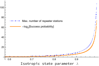
Figure 33: In this figure, we plot (a) the maximum allowed number of relay stations between Alice and Bob (shown in blue) and (b) $\log$(success probability) (in yellow) for the state $\rho^{I}_{AB}(p(\lambda^{n+1}),2)$ to remain entangled. (Color online)

It is observed that the number of allowed repeater stations in the network depends on the information processing task that the network is executing. The number of allowed repeater stations increases with the increase in $\lambda$. Furthermore, the success probability of the information processing task decreases with an increase in the number of allowed repeater stations.

Appendix I Analysis of time-varying quantum networks

In general, the network parameters i.e., the number of nodes, edges, and edge weights may change with time. Let us denote such a time-varying network as $\mathscr{N}(G(\mathbb{V}(t),\mathbb{E}(t)))$. We say that two nodes $v_{i}$ and $v_{j}$ of a time-varying network are connected in the time interval $[t_{1},t_{2}]$ if $\exists~{}e_{ij}\in\mathbb{E}(t)$ with $p_{ij}\geq p_{\ast}~{}\forall t\in[t_{1},t_{2}]$. In the following example, we present the variation of link sparsity with time for the time-varying network shown in Fig. 34.

Example 5.

Consider a network $\mathscr{N}(G(\mathbb{V}(t),\mathbb{E}(t)))$ whose vertices and edges are evolving in time as shown in Fig. 34. We assume that for $e_{ij}\in\mathbb{E}(t)$,

$$p_{ij}(t+1)\coloneqq\begin{cases}w\mathrm{e}^{-kt}~{}p_{ij}(t)&\text{for $w\mathrm{e}^{-kt}~{}p_{ij}(t)>p_{\ast}$},\\ 0&\text{otherwise},\end{cases}$$ (96)

where $w=0.9,p_{\ast}=0.05,k=0.3$ sec^-1 and $t\in[1,4]$.

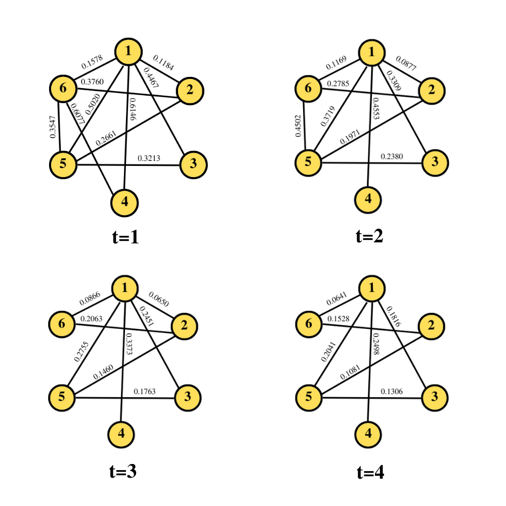
Figure 34: We present a time varying mesh network with $6$ nodes as a series of $4$ static graphs. We consider the network topology at times $t\in\{1,2,3,4\}.$ In this network, the edges $e_{ij}$ connecting nodes $v_{i}$ and $v_{j}$ denote the success probabilities $p_{ij}$ of transferring some resource between the $v_{i}$ and $v_{j}$. The success probability $p_{ij}$ evolves in time following Eq. (96). (Color online)

For such a network, we have the variation of the link sparsity with time as

$t$ (sec)	1	2	3	4
$\Upsilon(\mathscr{N})$	0.4445	0.5	0.5556	0.6112

Table 2: Link sparsity for time-evolving graph

We observe from Table 2 that for the network shown in Fig 34, the link sparsity increases with time and the network becomes less robust.

References

- Dowling and Milburn (2003) Jonathan P Dowling and Gerard J Milburn, “Quantum technology: the second quantum revolution,” Philosophical Transactions of the Royal Society of London. Series A: Mathematical, Physical and Engineering Sciences 361, 1655–1674 (2003).
- Kimble (2008) H Jeff Kimble, “The quantum internet,” Nature 453, 1023–1030 (2008).
- Wehner et al. (2018) Stephanie Wehner, David Elkouss, and Ronald Hanson, “Quantum internet: A vision for the road ahead,” Science 362, eaam9288 (2018).
- Bennett and Brassard (1984) C. H. Bennett and G. Brassard, “Quantum Cryptography: Public Key Distribution and Coin Tossing,” Proceedings of the IEEE International Conference on Computers, Systems and Signal Processing , 175–179 (1984).
- Ekert (1991) Artur K. Ekert, “Quantum cryptography based on Bell’s theorem,” Physical Review Letters 67, 661–663 (1991).
- Acín et al. (2007) Antonio Acín, Nicolas Brunner, Nicolas Gisin, Serge Massar, Stefano Pironio, and Valerio Scarani, “Device-independent security of quantum cryptography against collective attacks,” Physical Review Letters 98, 230501 (2007).
- Renner (2008) Renato Renner, “Security of quantum key distribution,” International Journal of Quantum Information 6, 1–127 (2008).
- Barrett et al. (2013) Jonathan Barrett, Roger Colbeck, and Adrian Kent, “Memory Attacks on Device-Independent Quantum Cryptography,” Physical Review Letters 110, 010503 (2013).
- Lucamarini et al. (2018) Marco Lucamarini, Zhiliang L Yuan, James F Dynes, and Andrew J Shields, “Overcoming the rate–distance limit of quantum key distribution without quantum repeaters,” Nature 557, 400–403 (2018).
- Arnon-Friedman et al. (2018) Rotem Arnon-Friedman, Frédéric Dupuis, Omar Fawzi, Renato Renner, and Thomas Vidick, “Practical device-independent quantum cryptography via entropy accumulation,” Nature communications 9, 459 (2018).
- Das (2019) Siddhartha Das, “Bipartite Quantum Interactions: Entangling and Information Processing Abilities,” (2019), arXiv:1901.05895.
- Xu et al. (2020) Feihu Xu, Xiongfeng Ma, Qiang Zhang, Hoi-Kwong Lo, and Jian-Wei Pan, “Secure quantum key distribution with realistic devices,” Reviews of Modern Physics 92, 025002 (2020).
- Das et al. (2021) Siddhartha Das, Stefan Bäuml, Marek Winczewski, and Karol Horodecki, “Universal Limitations on Quantum Key Distribution over a Network,” Physical Review X 11, 041016 (2021).
- Shor (1994) Peter W Shor, “Algorithms for quantum computation: discrete logarithms and factoring,” in Proceedings 35th annual symposium on foundations of computer science (Ieee, 1994) pp. 124–134.
- Jozsa (1997) Richard Jozsa, “Entanglement and quantum computation,” (1997), arXiv quant-ph/9707034.
- Grover (1996) Lov K Grover, “A fast quantum mechanical algorithm for database search,” in Proceedings of the twenty-eighth annual ACM symposium on Theory of computing (1996) pp. 212–219.
- Knill et al. (2001) Emanuel Knill, Raymond Laflamme, and Gerald J Milburn, “A scheme for efficient quantum computation with linear optics,” Nature 409, 46–52 (2001).
- Childs et al. (2003) Andrew M Childs, Richard Cleve, Enrico Deotto, Edward Farhi, Sam Gutmann, and Daniel A Spielman, “Exponential algorithmic speedup by a quantum walk,” in Proceedings of the thirty-fifth annual ACM symposium on Theory of computing (2003) pp. 59–68.
- Braunstein and van Loock (2005) Samuel L. Braunstein and Peter van Loock, “Quantum information with continuous variables,” Reviews of Modern Physics 77, 513–577 (2005).
- Menicucci et al. (2006) Nicolas C. Menicucci, Peter van Loock, Mile Gu, Christian Weedbrook, Timothy C. Ralph, and Michael A. Nielsen, “Universal Quantum Computation with Continuous-Variable Cluster States,” Physical Review Letters 97, 110501 (2006).
- Aaronson and Arkhipov (2011) Scott Aaronson and Alex Arkhipov, “The computational complexity of linear optics,” in Proceedings of the forty-third annual ACM symposium on Theory of computing (2011) pp. 333–342.
- Cirac et al. (1999) J Ignacio Cirac, AK Ekert, Susana F Huelga, and Chiara Macchiavello, “Distributed quantum computation over noisy channels,” Physical Review A 59, 4249 (1999).
- Fitzi et al. (2001) Matthias Fitzi, Nicolas Gisin, and Ueli Maurer, “Quantum Solution to the Byzantine Agreement Problem,” Physical Review Letters 87, 217901 (2001).
- Raussendorf and Briegel (2001) Robert Raussendorf and Hans J. Briegel, “A One-Way Quantum Computer,” Physical Review Letters 86, 5188–5191 (2001).
- Beals et al. (2013) Robert Beals, Stephen Brierley, Oliver Gray, Aram W Harrow, Samuel Kutin, Noah Linden, Dan Shepherd, and Mark Stather, “Efficient distributed quantum computing,” Proceedings of the Royal Society A: Mathematical, Physical and Engineering Sciences 469, 20120686 (2013).
- Lim et al. (2005) Yuan Liang Lim, Almut Beige, and Leong Chuan Kwek, “Repeat-until-success Linear Optics Distributed Quantum Computing,” Physical Review Letters 95, 030505 (2005).
- Liu et al. (2023) Xiao Liu, Xiao-Min Hu, Tian-Xiang Zhu, Chao Zhang, Yi-Xin Xiao, Jia-Le Miao, Zhong-Wen Ou, Bi-Heng Liu, Zong-Quan Zhou, Chuan-Feng Li, and Guang-Can Guo, “Distributed quantum computing over 7.0 km,” (2023), arXiv:2307.15634.
- Childs (2001) Andrew M Childs, “Secure assisted quantum computation,” (2001), arXiv quant-ph/0111046.
- Giovannetti et al. (2008) Vittorio Giovannetti, Seth Lloyd, and Lorenzo Maccone, “Quantum private queries,” Physical Review Letters 100, 230502 (2008).
- Broadbent et al. (2009) Anne Broadbent, Joseph Fitzsimons, and Elham Kashefi, “Universal blind quantum computation,” in 2009 50th annual IEEE symposium on foundations of computer science (IEEE, 2009) pp. 517–526.
- Das and Siopsis (2021) Siddhartha Das and George Siopsis, “Practically secure quantum position verification,” New Journal of Physics 23, 063069 (2021).
- Bollinger et al. (1996) J. J . Bollinger, Wayne M. Itano, D. J. Wineland, and D. J. Heinzen, “Optimal frequency measurements with maximally correlated states,” Physical Review A 54, R4649–R4652 (1996).
- Giovannetti et al. (2004) Vittorio Giovannetti, Seth Lloyd, and Lorenzo Maccone, “Quantum-enhanced measurements: beating the standard quantum limit,” Science 306, 1330–1336 (2004).
- Giovannetti et al. (2006) Vittorio Giovannetti, Seth Lloyd, and Lorenzo Maccone, “Quantum Metrology,” Physical Review Letters 96, 010401 (2006).
- Budker and Romalis (2007) Dmitry Budker and Michael Romalis, “Optical magnetometry,” Nature Physics 3, 227–234 (2007).
- Taylor et al. (2008) Jacob M Taylor, Paola Cappellaro, Lilian Childress, Liang Jiang, Dmitry Budker, PR Hemmer, Amir Yacoby, Ronald Walsworth, and MD Lukin, “High-sensitivity diamond magnetometer with nanoscale resolution,” Nature Physics 4, 810–816 (2008).
- Degen et al. (2017) C. L. Degen, F. Reinhard, and P. Cappellaro, “Quantum sensing,” Reviews of Modern Physics 89, 035002 (2017).
- Meyer et al. (2023) Johannes Jakob Meyer, Sumeet Khatri, Daniel Stilck França, Jens Eisert, and Philippe Faist, “Quantum metrology in the finite-sample regime,” (2023), arXiv:2307.06370.
- Chuang (2000) Isaac L. Chuang, “Quantum Algorithm for Distributed Clock Synchronization,” Physical Review Letters 85, 2006–2009 (2000).
- Jozsa et al. (2000) Richard Jozsa, Daniel S. Abrams, Jonathan P. Dowling, and Colin P. Williams, “Quantum Clock Synchronization Based on Shared Prior Entanglement,” Physical Review Letters 85, 2010–2013 (2000).
- Giovannetti et al. (2001) Vittorio Giovannetti, Seth Lloyd, and Lorenzo Maccone, “Quantum-enhanced positioning and clock synchronization,” Nature 412, 417–419 (2001).
- Bennett and Wiesner (1992) Charles H. Bennett and Stephen J. Wiesner, “Communication via one-and two-particle operators on Einstein-Podolsky-Rosen states,” Physical Review Letters 69, 2881–2884 (1992).
- Bennett et al. (1996a) Charles H Bennett, Gilles Brassard, Sandu Popescu, Benjamin Schumacher, John A Smolin, and William K Wootters, “Purification of noisy entanglement and faithful teleportation via noisy channels,” Physical Review Letters 76, 722 (1996a).
- Schumacher (1996) Benjamin Schumacher, “Sending entanglement through noisy quantum channels,” Physical Review A 54, 2614–2628 (1996).
- Mattle et al. (1996) Klaus Mattle, Harald Weinfurter, Paul G. Kwiat, and Anton Zeilinger, “Dense Coding in Experimental Quantum Communication,” Physical Review Letters 76, 4656–4659 (1996).
- van Enk et al. (1997) S. J. van Enk, J. I. Cirac, and P. Zoller, “Ideal Quantum Communication over Noisy Channels: A Quantum Optical Implementation,” Physical Review Letters 78, 4293–4296 (1997).
- Bose (2003) Sougato Bose, “Quantum Communication through an Unmodulated Spin Chain,” Physical Review Letters 91, 207901 (2003).
- van Loock et al. (2006) P. van Loock, T. D. Ladd, K. Sanaka, F. Yamaguchi, Kae Nemoto, W. J. Munro, and Y. Yamamoto, “Hybrid Quantum Repeater Using Bright Coherent Light,” Physical Review Letters 96, 240501 (2006).
- Zhang et al. (2017) Wei Zhang, Dong-Sheng Ding, Yu-Bo Sheng, Lan Zhou, Bao-Sen Shi, and Guang-Can Guo, “Quantum Secure Direct Communication with Quantum Memory,” Physical Review Letters 118, 220501 (2017).
- Das et al. (2020) Siddhartha Das, Stefan Bäuml, and Mark M. Wilde, “Entanglement and secret-key-agreement capacities of bipartite quantum interactions and read-only memory devices,” Physical Review A 101, 012344 (2020).
- Kaur et al. (2019) Eneet Kaur, Siddhartha Das, Mark M Wilde, and Andreas Winter, “Extendibility limits the performance of quantum processors,” Physical Review Letters 123, 070502 (2019).
- Bhaskar et al. (2020) M. K. Bhaskar, R. Riedinger, B. Machielse, D. S. Levonian, C. T. Nguyen, E. N. Knall, H. Park, D. Englund, M. Lončar, D. D. Sukachev, and M. D. Lukin, “Experimental demonstration of memory-enhanced quantum communication,” Nature 580, 60–64 (2020).
- Cheong et al. (2022) Jian Wei Cheong, Andri Pradana, and Lock Yue Chew, “Communication advantage of quantum compositions of channels from non-Markovianity,” Physical Review A 106, 052410 (2022).
- Liu et al. (2002) X. S. Liu, G. L. Long, D. M. Tong, and Feng Li, “General scheme for superdense coding between multiparties,” Physical Review A 65, 022304 (2002).
- Das and Wilde (2019) Siddhartha Das and Mark M. Wilde, “Quantum rebound capacity,” Physical Review A 100, 030302 (2019).
- Bennett et al. (1993) Charles H. Bennett, Gilles Brassard, Claude Crépeau, Richard Jozsa, Asher Peres, and William K. Wootters, “Teleporting an unknown quantum state via dual classical and Einstein-Podolsky-Rosen channels,” Physical Review Letters 70, 1895–1899 (1993).
- Bouwmeester et al. (1997) Dik Bouwmeester, Jian-Wei Pan, Klaus Mattle, Manfred Eibl, Harald Weinfurter, and Anton Zeilinger, “Experimental quantum teleportation,” Nature 390, 575–579 (1997).
- Furusawa et al. (1998) Akira Furusawa, Jens Lykke Sørensen, Samuel L Braunstein, Christopher A Fuchs, H Jeff Kimble, and Eugene S Polzik, “Unconditional quantum teleportation,” Science 282, 706–709 (1998).
- Horodecki et al. (1996) Ryszard Horodecki, Michał Horodecki, and Paweł Horodecki, “Teleportation, Bell’s inequalities and inseparability,” Physics Letters A 222, 21–25 (1996).
- van Loock and Braunstein (2000) P. van Loock and Samuel L. Braunstein, “Multipartite Entanglement for Continuous Variables: A Quantum Teleportation Network,” Physical Review Letters 84, 3482–3485 (2000).
- Pironio et al. (2010) S. Pironio, A. Acín, S. Massar, A. Boyer de la Giroday, D. N. Matsukevich, P. Maunz, S. Olmschenk, D. Hayes, L. Luo, T. A. Manning, and C. Monroe, “Random numbers certified by Bell’s theorem,” Nature 464, 1021–1024 (2010).
- Colbeck and Kent (2011) Roger Colbeck and Adrian Kent, “Private randomness expansion with untrusted devices,” Journal of Physics A: Mathematical and Theoretical 44, 095305 (2011).
- Acín et al. (2012) Antonio Acín, Serge Massar, and Stefano Pironio, “Randomness versus nonlocality and entanglement,” Physical Review Letters 108, 100402 (2012).
- Colbeck and Renner (2012) Roger Colbeck and Renato Renner, “Free randomness can be amplified,” Nature Physics 8, 450–453 (2012).
- Yang et al. (2019) Dong Yang, Karol Horodecki, and Andreas Winter, “Distributed Private Randomness Distillation,” Physical Review Letters 123, 170501 (2019).
- Schrödinger (1935) Erwin Schrödinger, “Discussion of Probability Relations between Separated Systems,” Mathematical Proceedings of the Cambridge Philosophical Society 31, 555–563 (1935).
- Horodecki et al. (2009a) Ryszard Horodecki, Paweł Horodecki, Michał Horodecki, and Karol Horodecki, “Quantum entanglement,” Reviews of modern physics 81, 865 (2009a).
- Pan et al. (2012) Jian-Wei Pan, Zeng-Bing Chen, Chao-Yang Lu, Harald Weinfurter, Anton Zeilinger, and Marek Żukowski, “Multiphoton entanglement and interferometry,” Reviews of Modern Physics 84, 777–838 (2012).
- Das et al. (2018a) Siddhartha Das, Sumeet Khatri, and Jonathan P Dowling, “Robust quantum network architectures and topologies for entanglement distribution,” Physical Review A 97, 012335 (2018a).
- Bäuml et al. (2018) Stefan Bäuml, Siddhartha Das, and Mark M. Wilde, “Fundamental Limits on the Capacities of Bipartite Quantum Interactions,” Physical Review Letters 121, 250504 (2018).
- Friis et al. (2019) Nicolai Friis, Giuseppe Vitagliano, Mehul Malik, and Marcus Huber, “Entanglement certification from theory to experiment,” Nature Reviews Physics 1, 72–87 (2019).
- Xing et al. (2023) Junjing Xing, Tianfeng Feng, Zhaobing Fan, Haitao Ma, Kishor Bharti, Dax Enshan Koh, and Yunlong Xiao, “Fundamental Limitations on Communication over a Quantum Network,” (2023), arXiv:2306.04983.
- Khatri (2022a) Sumeet Khatri, “On the design and analysis of near-term quantum network protocols using Markov decision processes,” AVS Quantum Science 4 (2022a).
- Bell (1964) John S Bell, “On the Einstein Podolsky Rosen paradox,” Physics Physique Fizika 1, 195 (1964).
- Clauser et al. (1969) John F Clauser, Michael A Horne, Abner Shimony, and Richard A Holt, “Proposed experiment to test local hidden-variable theories,” Physical Review Letters 23, 880 (1969).
- Brunner et al. (2014) Nicolas Brunner, Daniel Cavalcanti, Stefano Pironio, Valerio Scarani, and Stephanie Wehner, “Bell nonlocality,” Review of Modern Physics 86, 419–478 (2014).
- Tavakoli et al. (2022) Armin Tavakoli, Alejandro Pozas-Kerstjens, Ming-Xing Luo, and Marc-Olivier Renou, “Bell nonlocality in networks,” Reports on Progress in Physics 85, 056001 (2022).
- Aspect et al. (1982) Alain Aspect, Jean Dalibard, and Gérard Roger, “Experimental test of Bell’s inequalities using time-varying analyzers,” Physical Review Letters 49, 1804 (1982).
- Hensen et al. (2015) B. Hensen, H. Bernien, A. E. Dréau, A. Reiserer, N. Kalb, M. S. Blok, J. Ruitenberg, R. F. L. Vermeulen, R. N. Schouten, C. Abellán, W. Amaya, V. Pruneri, M. W. Mitchell, M. Markham, D. J. Twitchen, D. Elkouss, S. Wehner, T. H. Taminiau, and R. Hanson, “Loophole-free Bell inequality violation using electron spins separated by 1.3 kilometres,” Nature 526, 682–686 (2015).
- Giustina et al. (2015) Marissa Giustina, Marijn A. M. Versteegh, Sören Wengerowsky, Johannes Handsteiner, Armin Hochrainer, Kevin Phelan, Fabian Steinlechner, Johannes Kofler, Jan-Åke Larsson, Carlos Abellán, Waldimar Amaya, Valerio Pruneri, Morgan W. Mitchell, Jörn Beyer, Thomas Gerrits, Adriana E. Lita, Lynden K. Shalm, Sae Woo Nam, Thomas Scheidl, Rupert Ursin, Bernhard Wittmann, and Anton Zeilinger, “Significant-loophole-free test of bell’s theorem with entangled photons,” Physical Review Letters 115, 250401 (2015).
- Home et al. (2015) Dipankar Home, Debashis Saha, and Siddhartha Das, “Multipartite Bell-type inequality by generalizing Wigner’s argument,” Physical Review A 91, 012102 (2015).
- Luo (2022) Ming-Xing Luo, “Fully device-independent model on quantum networks,” Physical Review Research 4, 013203 (2022).
- Bjerrum et al. (2023) Anders J. E. Bjerrum, Jonatan B. Brask, Jonas S. Neergaard-Nielsen, and Ulrik L. Andersen, “Proposal for a long-distance nonlocality test with entanglement swapping and displacement-based measurements,” Physical Review A 107, 052611 (2023).
- Streltsov et al. (2015) Alexander Streltsov, Uttam Singh, Himadri Shekhar Dhar, Manabendra Nath Bera, and Gerardo Adesso, “Measuring Quantum Coherence with Entanglement,” Physical Review Letters 115, 020403 (2015).
- Yao et al. (2015) Yao Yao, Xing Xiao, Li Ge, and C. P. Sun, “Quantum coherence in multipartite systems,” Physical Review A 92, 022112 (2015).
- Singh et al. (2021) Uttam Singh, Siddhartha Das, and Nicolas J. Cerf, “Partial order on passive states and Hoffman majorization in quantum thermodynamics,” Physical Review Reserach 3, 033091 (2021).
- Streltsov et al. (2017) Alexander Streltsov, Gerardo Adesso, and Martin B. Plenio, “Colloquium: Quantum coherence as a resource,” Review of Modern Physics 89, 041003 (2017).
- Valivarthi et al. (2020) Raju Valivarthi, Samantha I. Davis, Cristián Peña, Si Xie, Nikolai Lauk, Lautaro Narváez, Jason P. Allmaras, Andrew D. Beyer, Yewon Gim, Meraj Hussein, George Iskander, Hyunseong Linus Kim, Boris Korzh, Andrew Mueller, Mandy Rominsky, Matthew Shaw, Dawn Tang, Emma E. Wollman, Christoph Simon, Panagiotis Spentzouris, Daniel Oblak, Neil Sinclair, and Maria Spiropulu, “Teleportation systems toward a quantum internet,” PRX Quantum 1, 020317 (2020).
- Wang et al. (2014) Shuang Wang, Wei Chen, Zhen-Qiang Yin, Hong-Wei Li, De-Yong He, Yu-Hu Li, Zheng Zhou, Xiao-Tian Song, Fang-Yi Li, Dong Wang, Hua Chen, Yun-Guang Han, Jing-Zheng Huang, Jun-Fu Guo, Peng-Lei Hao, Mo Li, Chun-Mei Zhang, Dong Liu, Wen-Ye Liang, Chun-Hua Miao, Ping Wu, Guang-Can Guo, and Zheng-Fu Han, “Field and long-term demonstration of a wide area quantum key distribution network,” 22, 21739–21756 (2014).
- Stucki et al. (2011) D Stucki, M Legré, F Buntschu, B Clausen, N Felber, N Gisin, L Henzen, P Junod, G Litzistorf, P Monbaron, L Monat, J-B Page, D Perroud, G Ribordy, A Rochas, S Robyr, J Tavares, R Thew, P Trinkler, S Ventura, R Voirol, N Walenta, and H Zbinden, “Long-term performance of the SwissQuantum quantum key distribution network in a field environment,” New Journal of Physics 13, 123001 (2011).
- Ofek et al. (2016) Nissim Ofek, Andrei Petrenko, Reinier Heeres, Philip Reinhold, Zaki Leghtas, Brian Vlastakis, Yehan Liu, Luigi Frunzio, S. M. Girvin, L. Jiang, Mazyar Mirrahimi, M. H. Devoret, and R. J. Schoelkopf, “Extending the lifetime of a quantum bit with error correction in superconducting circuits,” Nature 536, 441–445 (2016).
- Das et al. (2018b) Siddhartha Das, Sumeet Khatri, George Siopsis, and Mark M. Wilde, “Fundamental limits on quantum dynamics based on entropy change,” Journal of Mathematical Physics 59 (2018b), 10.1063/1.4997044.
- Wang et al. (2022) Chenlu Wang, Xuegang Li, Huikai Xu, Zhiyuan Li, Junhua Wang, Zhen Yang, Zhenyu Mi, Xuehui Liang, Tang Su, Chuhong Yang, Guangyue Wang, Wenyan Wang, Yongchao Li, Mo Chen, Chengyao Li, Kehuan Linghu, Jiaxiu Han, Yingshan Zhang, Yulong Feng, Yu Song, Teng Ma, Jingning Zhang, Ruixia Wang, Peng Zhao, Weiyang Liu, Guangming Xue, Yirong Jin, and Haifeng Yu, “Towards practical quantum computers: Transmon qubit with a lifetime approaching 0.5 milliseconds,” npj Quantum Information 8, 3 (2022).
- Kim et al. (2023) Youngseok Kim, Andrew Eddins, Sajant Anand, Ken Xuan Wei, Ewout van den Berg, Sami Rosenblatt, Hasan Nayfeh, Yantao Wu, Michael Zaletel, Kristan Temme, and Abhinav Kandala, “Evidence for the utility of quantum computing before fault tolerance,” Nature 618, 500–505 (2023).
- Azuma et al. (2015) Koji Azuma, Kiyoshi Tamaki, and Hoi-Kwong Lo, “All-photonic quantum repeaters,” Nature Communications 6, 1–7 (2015).
- Ecker et al. (2022) Sebastian Ecker, Johannes Pseiner, Jorge Piris, and Martin Bohmann, “Advances in entanglement-based QKD for space applications,” (2022), arXiv:2210.02229.
- Lu et al. (2022) Chao-Yang Lu, Yuan Cao, Cheng-Zhi Peng, and Jian-Wei Pan, “Micius quantum experiments in space,” Reviews of Modern Physics 94, 035001 (2022).
- Liu et al. (2022) Tonghua Liu, Shuo Cao, Sixuan Zhang, Hao Zheng, and Xiaobao Liu, “Satellite-based continuous-variable quantum key distribution under the Earth’s gravitational field,” Quantum Information Processing 21, 397 (2022).
- Kaur et al. (2022) Eneet Kaur, Karol Horodecki, and Siddhartha Das, “Upper bounds on device-independent quantum key distribution rates in static and dynamic scenarios,” Physical Review Applied 18, 054033 (2022).
- Briegel et al. (1998) H-J Briegel, Wolfgang Dür, Juan I Cirac, and Peter Zoller, “Quantum repeaters: the role of imperfect local operations in quantum communication,” Physical Review Letters 81, 5932 (1998).
- Buscemi et al. (2016) Francesco Buscemi, Siddhartha Das, and Mark M. Wilde, “Approximate reversibility in the context of entropy gain, information gain, and complete positivity,” Physical Review A 93, 062314 (2016).
- Len et al. (2022) Yink Loong Len, Tuvia Gefen, Alex Retzker, and Jan Kołodyński, “Quantum metrology with imperfect measurements,” Nature Communications 13, 6971 (2022).
- Sadhu and Das (2023) Abhishek Sadhu and Siddhartha Das, “Testing of quantum nonlocal correlations under constrained free will and imperfect detectors,” Physical Review A 107, 012212 (2023).
- Fuchs and Peres (1996) Christopher A Fuchs and Asher Peres, “Quantum-state disturbance versus information gain: Uncertainty relations for quantum information,” Physical Review A 53, 2038 (1996).
- Wootters and Zurek (1982) William K Wootters and Wojciech H Zurek, “A single quantum cannot be cloned,” Nature 299, 802–803 (1982).
- Dür et al. (1999) Wolfgang Dür, H-J Briegel, Juan Ignacio Cirac, and Peter Zoller, “Quantum repeaters based on entanglement purification,” Physical Review A 59, 169 (1999).
- Zhan et al. (2023) Yuan Zhan, Paul Hilaire, Edwin Barnes, Sophia E Economou, and Shuo Sun, “Performance analysis of quantum repeaters enabled by deterministically generated photonic graph states,” Quantum 7, 924 (2023).
- Khatri et al. (2019) Sumeet Khatri, Corey T Matyas, Aliza U Siddiqui, and Jonathan P Dowling, “Practical figures of merit and thresholds for entanglement distribution in quantum networks,” Physical Review Research 1, 023032 (2019).
- Shchukin and van Loock (2022) Evgeny Shchukin and Peter van Loock, “Optimal Entanglement Swapping in Quantum Repeaters,” Physical Review Letters 128, 150502 (2022).
- Xie et al. (2022) Yuan-Mei Xie, Yu-Shuo Lu, Chen-Xun Weng, Xiao-Yu Cao, Zhao-Ying Jia, Yu Bao, Yang Wang, Yao Fu, Hua-Lei Yin, and Zeng-Bing Chen, “Breaking the rate-loss bound of quantum key distribution with asynchronous two-photon interference,” PRX Quantum 3, 020315 (2022).
- Horodecki et al. (2022) Karol Horodecki, Marek Winczewski, and Siddhartha Das, “Fundamental limitations on the device-independent quantum conference key agreement,” Physical Review A 105, 022604 (2022).
- Li et al. (2023) Chen-Long Li, Yao Fu, Wen-Bo Liu, Yuan-Mei Xie, Bing-Hong Li, Min-Gang Zhou, Hua-Lei Yin, and Zeng-Bing Chen, “Breaking the rate-distance limitation of measurement-device-independent quantum secret sharing,” Physical Review Research 5, 033077 (2023).
- Kamin et al. (2023) Lars Kamin, Evgeny Shchukin, Frank Schmidt, and Peter van Loock, “Exact rate analysis for quantum repeaters with imperfect memories and entanglement swapping as soon as possible,” Physical Review Research 5, 023086 (2023).
- Li et al. (2022) Chen-Long Li, Yao Fu, Wen-Bo Liu, Yuan-Mei Xie, Bing-Hong Li, Min-Gang Zhou, Hua-Lei Yin, and Zeng-Bing Chen, “Breaking universal limitations on quantum conference key agreement without quantum memory,” (2022), arXiv:2212.05226.
- Zukowski et al. (1993) Marek Zukowski, Anton Zeilinger, Michael A Horne, and Aarthur K Ekert, “” event-ready-detectors” Bell experiment via entanglement swapping.” Physical Review Letters 71 (1993).
- Pan et al. (1998) Jian-Wei Pan, Dik Bouwmeester, Harald Weinfurter, and Anton Zeilinger, “Experimental Entanglement Swapping: Entangling Photons That Never Interacted,” Physical Review Letters 80, 3891–3894 (1998).
- Bose et al. (1998) S. Bose, V. Vedral, and P. L. Knight, “Multiparticle generalization of entanglement swapping,” Physical Review A 57, 822–829 (1998).
- Sen (De) Aditi Sen(De), Ujjwal Sen, Časlav Brukner, Vladimír Bužek, and Marek Żukowski, “Entanglement swapping of noisy states: A kind of superadditivity in nonclassicality,” Physical Review A 72, 042310 (2005).
- Deutsch et al. (1996) David Deutsch, Artur Ekert, Richard Jozsa, Chiara Macchiavello, Sandu Popescu, and Anna Sanpera, “Quantum privacy amplification and the security of quantum cryptography over noisy channels,” Physical Review Letters 77, 2818 (1996).
- Bose et al. (1999) S. Bose, V. Vedral, and P. L. Knight, “Purification via entanglement swapping and conserved entanglement,” Physical Review A 60, 194–197 (1999).
- Hu et al. (2021) Xiao-Min Hu, Cen-Xiao Huang, Yu-Bo Sheng, Lan Zhou, Bi-Heng Liu, Yu Guo, Chao Zhang, Wen-Bo Xing, Yun-Feng Huang, Chuan-Feng Li, and Guang-Can Guo, “Long-distance Entanglement Purification for Quantum Communication,” Physical Review Letters 126, 010503 (2021).
- Wang et al. (2021) Xingyu Wang, Chen Dong, Tianyi Wu, Kai Li, Boyu Deng, Lei Shi, and Shanghong Zhao, “Exploiting potentialities for space-based quantum communication network: satellite quantum modelling & downlink scheduling analysis,” (2021), arXiv:2106.00987.
- Aspelmeyer et al. (2003) Markus Aspelmeyer, Thomas Jennewein, Martin Pfennigbauer, Walter R Leeb, and Anton Zeilinger, “Long-distance quantum communication with entangled photons using satellites,” IEEE Journal of Selected Topics in Quantum Electronics 9, 1541–1551 (2003).
- Bedington et al. (2017) Robert Bedington, Juan Miguel Arrazola, and Alexander Ling, “Progress in satellite quantum key distribution,” npj Quantum Information 3, 30 (2017).
- Śliwa and Banaszek (2003) Cezary Śliwa and Konrad Banaszek, “Conditional preparation of maximal polarization entanglement,” Physical Review A 67, 030101 (2003).
- Azuma et al. (2021) Koji Azuma, Stefan Bäuml, Tim Coopmans, David Elkouss, and Boxi Li, “Tools for quantum network design,” AVS Quantum Science 3 (2021).
- Bopp et al. (2022) Julian M Bopp, Matthias Plock, Tim Turan, Gregor Pieplow, Sven Burger, and Tim Schröder, “’sawfish’photonic Crystal Cavity for Near-Unity Emitter-to-Fiber Interfacing in Quantum Network Applications,” (2022), arXiv:2210.04702.
- You et al. (2022) Xiang You, Ming-Yang Zheng, Si Chen, Run-Ze Liu, Jian Qin, Mo-Chi Xu, Zheng-Xuan Ge, Tung-Hsun Chung, Yu-Kun Qiao, Yang-Fan Jiang, Han-Sen Zhong, Ming-Cheng Chen, Hui Wang, Yu-Ming He, Xiu-Ping Xie, Hao Li, Li-Xing You, Christian Schneider, Juan Yin, Teng-Yun Chen, Mohamed Benyoucef, Yong-Heng Huo, Sven Höfling, Qiang Zhang, Chao-Yang Lu, and Jian-Wei Pan, “Quantum interference with independent single-photon sources over 300 km fiber,” Advanced Photonics 4, 066003 (2022).
- Bennett et al. (1992a) Charles H Bennett, François Bessette, Gilles Brassard, Louis Salvail, and John Smolin, “Experimental quantum cryptography,” Journal of cryptology 5, 3–28 (1992a).
- Scarani and Renner (2008) Valerio Scarani and Renato Renner, “Quantum Cryptography with Finite Resources: Unconditional Security Bound for Discrete-Variable Protocols with One-Way Postprocessing,” Physical Review Letters 100, 200501 (2008).
- Cai and Scarani (2009) Raymond YQ Cai and Valerio Scarani, “Finite-key analysis for practical implementations of quantum key distribution,” New Journal of Physics 11, 045024 (2009).
- Pearson (2004) David Pearson, “High-speed QKD reconciliation using forward error correction,” in AIP Conference Proceedings, Vol. 734 (American Institute of Physics, 2004) pp. 299–302.
- Yin et al. (2020) Juan Yin, Yu-Huai Li, Sheng-Kai Liao, Meng Yang, Yuan Cao, Liang Zhang, Ji-Gang Ren, Wen-Qi Cai, Wei-Yue Liu, Shuang-Lin Li, Rong Shu, Yong-Mei Huang, Lei Deng, Li Li, Qiang Zhang, Nai-Le Liu, Yu-Ao Chen, Chao-Yang Lu, Xiang-Bin Wang, Feihu Xu, Jian-Yu Wang, Cheng-Zhi Peng, Artur K. Ekert, and Jian-Wei Pan, “Entanglement-based secure quantum cryptography over 1,120 kilometres,” Nature 582, 501–505 (2020).
- West (2000) Douglas B. West, Introduction to Graph Theory - Second edition (Pearson, 2000).
- Tutte (2001) William Thomas Tutte, Graph theory, Vol. 21 (Cambridge university press, 2001).
- Barnes and Harary (1983) John A Barnes and Frank Harary, “Graph theory in network analysis,” Social networks 5, 235–244 (1983).
- Broadbent and Hammersley (1957) S. R. Broadbent and J. M. Hammersley, “Percolation processes: I. Crystals and mazes,” Mathematical Proceedings of the Cambridge Philosophical Society 53, 629–641 (1957).
- Stauffer and Aharony (2018) Dietrich Stauffer and Ammon Aharony, Introduction to percolation theory (CRC press, 2018).
- Beffara and Sidoravicius (2005) Vincent Beffara and Vladas Sidoravicius, “Percolation theory,” (2005), arXiv:math/0507220.
- AI (2021) Google Quantum AI, “Quantum Computer Datasheet,” https://quantumai.google/hardware/datasheet/weber.pdf (2021).
- (141) IBM Quantum (2022), “ibmwashington,” https://quantum-computing.ibm.com/services/resources (2022).
- Begušić et al. (2023) Tomislav Begušić, Johnnie Gray, and Garnet Kin-Lic Chan, “Fast and converged classical simulations of evidence for the utility of quantum computing before fault tolerance,” (2023), arXiv:2308.05077.
- Computing (2020) Rigetti Computing, “Aspen-m-2 quantum processor,” https://qcs.rigetti.com/qpus (2020).
- (144) Monika Maciag-Kruszewska and ibmblogs, “Polish PSNC to Join IBM Quantum Network, Becoming First Hub in Central and Eastern Europe,” https://www.ibm.com/blogs/southeast-europe/poland-psnc-ibm-quantum-hub/.
- Halder et al. (2022) Pritam Halder, Ratul Banerjee, Srijon Ghosh, Amit Kumar Pal, and Aditi Sen(De), “Circulating genuine multiparty entanglement in a quantum network,” Physical Review A 106, 032604 (2022).
- Iñesta et al. (2023) Álvaro G Iñesta, Gayane Vardoyan, Lara Scavuzzo, and Stephanie Wehner, “Optimal entanglement distribution policies in homogeneous repeater chains with cutoffs,” npj Quantum Information 9, 46 (2023).
- Bugalho et al. (2023) Luís Bugalho, Bruno C Coutinho, Francisco A Monteiro, and Yasser Omar, “Distributing multipartite entanglement over noisy quantum networks,” Quantum 7, 920 (2023).
- Khatri (2021) Sumeet Khatri, “Policies for elementary links in a quantum network,” Quantum 5, 537 (2021).
- Lee et al. (2022) Yuan Lee, Eric Bersin, Axel Dahlberg, Stephanie Wehner, and Dirk Englund, “A quantum router architecture for high-fidelity entanglement flows in quantum networks,” npj Quantum Information 8, 75 (2022).
- Horodecki and Horodecki (1999) Michał Horodecki and Paweł Horodecki, “Reduction criterion of separability and limits for a class of distillation protocols,” Physical Review A 59, 4206–4216 (1999).
- Farkas et al. (2021) Máté Farkas, Maria Balanzó-Juandó, Karol Łukanowski, Jan Kołodyński, and Antonio Acín, “Bell nonlocality is not sufficient for the security of standard device-independent quantum key distribution protocols,” Physical Review Letters 127, 050503 (2021).
- Werner (1989) Reinhard F Werner, “Quantum states with Einstein-Podolsky-Rosen correlations admitting a hidden-variable model,” Physical Review A 40, 4277 (1989).
- Leiserson et al. (2009) Charles Eric Leiserson, Ronald L Rivest, Thomas H Cormen, and Clifford Stein, Introduction to Algorithms - Third edition (MIT press Cambridge, MA, USA, 2009).
- Bennett et al. (1992b) Charles H. Bennett, Gilles Brassard, and N. David Mermin, “Quantum cryptography without Bell’s theorem,” Physical Review Letters 68, 557–559 (1992b).
- Bäuml et al. (2015) Stefan Bäuml, Matthias Christandl, Karol Horodecki, and Andreas Winter, “Limitations on quantum key repeaters,” Nature communications 6, 6908 (2015).
- Sangouard et al. (2011) Nicolas Sangouard, Christoph Simon, Hugues De Riedmatten, and Nicolas Gisin, “Quantum repeaters based on atomic ensembles and linear optics,” Reviews of Modern Physics 83, 33 (2011).
- Fitzsimons (2017) Joseph F Fitzsimons, “Private quantum computation: an introduction to blind quantum computing and related protocols,” npj Quantum Information 3, 23 (2017).
- Steffen et al. (2016) Matthias Steffen, Jay M Gambetta, and Jerry M Chow, “Progress, status, and prospects of superconducting qubits for quantum computing,” in 2016 46th European Solid-State Device Research Conference (ESSDERC) (IEEE, 2016) pp. 17–20.
- Horodecki et al. (1998) Michał Horodecki, Paweł Horodecki, and Ryszard Horodecki, “Mixed-state entanglement and distillation: Is there a “bound” entanglement in nature?” Physical Review Letters 80, 5239 (1998).
- Horodecki et al. (2009b) Karol Horodecki, Michal Horodecki, Pawel Horodecki, and Jonathan Oppenheim, “General paradigm for distilling classical key from quantum states,” IEEE Transactions on Information Theory 55, 1898–1929 (2009b).
- Schwonnek et al. (2021) René Schwonnek, Koon Tong Goh, Ignatius W Primaatmaja, Ernest Y-Z Tan, Ramona Wolf, Valerio Scarani, and Charles C-W Lim, “Device-independent quantum key distribution with random key basis,” Nature Communications 12, 1–8 (2021).
- Winczewski et al. (2022) Marek Winczewski, Tamoghna Das, and Karol Horodecki, “Limitations on a device-independent key secure against a nonsignaling adversary via squashed nonlocality,” Physical Review A 106, 052612 (2022).
- Duminil-Copin (2018) Hugo Duminil-Copin, “Introduction to Bernoulli percolation,” (2018).
- Horodecki et al. (1999) Michał Horodecki, Paweł Horodecki, and Ryszard Horodecki, “General teleportation channel, singlet fraction, and quasidistillation,” Physical Review A 60, 1888–1898 (1999).
- Press et al. (2007) David Press, Stephan Götzinger, Stephan Reitzenstein, Carolin Hofmann, Andreas Löffler, Martin Kamp, Alfred Forchel, and Yoshihisa Yamamoto, “Photon antibunching from a single quantum-dot-microcavity system in the strong coupling regime,” Physical Review Letters 98, 117402 (2007).
- Barros et al. (2009) HG Barros, A Stute, TE Northup, C Russo, PO Schmidt, and R Blatt, “Deterministic single-photon source from a single ion,” New Journal of Physics 11, 103004 (2009).
- Altepeter et al. (2005) Joseph B Altepeter, Evan R Jeffrey, and Paul G Kwiat, “Phase-compensated ultra-bright source of entangled photons,” Optics Express 13, 8951–8959 (2005).
- Bennett et al. (1997) Charles H. Bennett, David P. DiVincenzo, and John A. Smolin, “Capacities of Quantum Erasure Channels,” Physical Review Letters 78, 3217–3220 (1997).
- Goodenough et al. (2016) K Goodenough, D Elkouss, and S Wehner, “Assessing the performance of quantum repeaters for all phase-insensitive gaussian bosonic channels,” New Journal of Physics 18, 063005 (2016).
- Pirandola et al. (2017) Stefano Pirandola, Riccardo Laurenza, Carlo Ottaviani, and Leonardo Banchi, “Fundamental limits of repeaterless quantum communications,” Nature Communications 8, 15043 (2017).
- Wilde et al. (2017) Mark M. Wilde, Marco Tomamichel, and Mario Berta, “Converse bounds for private communication over quantum channels,” IEEE Transactions on Information Theory 63, 1792–1817 (2017), arXiv:1602.08898.
- Wang et al. (2018) Xiang-Bin Wang, Zong-Wen Yu, and Xiao-Long Hu, “Twin-field quantum key distribution with large misalignment error,” Physical Review A 98, 062323 (2018).
- Ma et al. (2018) Xiongfeng Ma, Pei Zeng, and Hongyi Zhou, “Phase-matching quantum key distribution,” Physical Review X 8, 031043 (2018).
- Zeng et al. (2020) Pei Zeng, Weijie Wu, and Xiongfeng Ma, “Symmetry-protected privacy: beating the rate-distance linear bound over a noisy channel,” Physical Review Applied 13, 064013 (2020).
- Xie et al. (2023) Yuan-Mei Xie, Chen-Xun Weng, Yu-Shuo Lu, Yao Fu, Yang Wang, Hua-Lei Yin, and Zeng-Bing Chen, “Scalable high-rate twin-field quantum key distribution networks without constraint of probability and intensity,” Physical Review A 107, 042603 (2023).
- Zhou et al. (2023) Lai Zhou, Jinping Lin, Yuan-Mei Xie, Yu-Shuo Lu, Yumang Jing, Hua-Lei Yin, and Zhiliang Yuan, “Experimental Quantum Communication Overcomes the Rate-Loss Limit without Global Phase Tracking,” Physical Review Letters 130, 250801 (2023).
- Albert et al. (2000) Réka Albert, Hawoong Jeong, and Albert-László Barabási, “Error and attack tolerance of complex networks,” Nature 406, 378–382 (2000).
- Callaway et al. (2000) Duncan S Callaway, Mark EJ Newman, Steven H Strogatz, and Duncan J Watts, “Network robustness and fragility: Percolation on random graphs,” Physical Review Letters 85, 5468 (2000).
- Mohseni-Kabir et al. (2021) Arman Mohseni-Kabir, Mihir Pant, Don Towsley, Saikat Guha, and Ananthram Swami, “Percolation thresholds for robust network connectivity,” Journal of Statistical Mechanics: Theory and Experiment 2021, 013212 (2021).
- Freeman et al. (1979) Linton C Freeman, Douglas Roeder, and Robert R Mulholland, “Centrality in social networks: II. Experimental results,” Social networks 2, 119–141 (1979).
- Freeman (1977) Linton C Freeman, “A set of measures of centrality based on betweenness,” Sociometry , 35–41 (1977).
- Gini (1912) Corrado Gini, “Variabilità e mutabilità (Variability and Mutability),” C. Cuppini, Bologna , 156 (1912).
- Stallings (1984) William Stallings, “Local networks,” ACM Computing Surveys (CSUR) 16, 3–41 (1984).
- Green (1980) P Green, “An introduction to network architectures and protocols,” IEEE Transactions on Communications 28, 413–424 (1980).
- Watts and Strogatz (1998) Duncan J Watts and Steven H Strogatz, “Collective dynamics of ‘small-world’networks,” Nature 393, 440–442 (1998).
- Google ([Online]) Google, “Satellite network,” ([Online]).
- Barz et al. (2012) Stefanie Barz, Elham Kashefi, Anne Broadbent, Joseph F Fitzsimons, Anton Zeilinger, and Philip Walther, “Demonstration of blind quantum computing,” Science 335, 303–308 (2012).
- Zeilinger et al. (1997) Anton Zeilinger, Michael A. Horne, Harald Weinfurter, and Marek Żukowski, “Three-Particle Entanglements from Two Entangled Pairs,” Physical Review Letters 78, 3031–3034 (1997).
- de Bone et al. (2020) Sébastian de Bone, Runsheng Ouyang, Kenneth Goodenough, and David Elkouss, “Protocols for creating and distilling multipartite GHZ states with Bell pairs,” IEEE Transactions on Quantum Engineering 1, 1–10 (2020).
- Nation et al. (2021) Paul Nation, Hanhee Paik, Andrew Cross, and Zaira Nazario, “The IBM Quantum heavy hex lattice,” https://research.ibm.com/blog/heavy-hex-lattice (2021).
- Lawrence ([Online]) Kelvin Lawrence, “Air route data - and more!” ([Online]).
- (192) U.S. Department of Energy Office of Science, “National QIS Research Centers,” https://science.osti.gov/-/media/QIS/pdf/QuantumBrochure2021.pdf.
- Schoute et al. (2016) Eddie Schoute, Laura Mancinska, Tanvirul Islam, Iordanis Kerenidis, and Stephanie Wehner, “Shortcuts to quantum network routing,” (2016), arXiv:1610.05238.
- Chakraborty et al. (2019) Kaushik Chakraborty, Filip Rozpedek, Axel Dahlberg, and Stephanie Wehner, “Distributed routing in a quantum internet,” (2019), arXiv:1907.11630.
- Li et al. (2020) Changhao Li, Tianyi Li, Yi-Xiang Liu, and Paola Cappellaro, “Effective routing design for remote entanglement generation on quantum networks,” (2020), arXiv:2001.02204.
- Khatri (2022b) Sumeet Khatri, “On the design and analysis of near-term quantum network protocols using Markov decision processes,” AVS Quantum Science 4, 030501 (2022b), https://pubs.aip.org/avs/aqs/article-pdf/doi/10.1116/5.0084653/16493927/030501_1_online.pdf .
- Dijkstra (1959) Edsger W Dijkstra, “A note on two problems in connexion with graphs,” Numerische Mathematik 1, 269–271 (1959).
- Bennett et al. (1996b) Charles H Bennett, David P DiVincenzo, John A Smolin, and William K Wootters, “Mixed-state entanglement and quantum error correction,” Physical Review A 54, 3824 (1996b).
- Kraus (1971) Karl Kraus, “General state changes in quantum theory,” Annals of Physics 64, 311–335 (1971).
- Choi (1975) Man-Duen Choi, “Completely positive linear maps on complex matrices,” Linear Algebra and Its Applications 10, 285–290 (1975).
- Romero and Franco (2012) KM Fonseca Romero and R Lo Franco, “Simple non-Markovian microscopic models for the depolarizing channel of a single qubit,” Physica Scripta 86, 065004 (2012).
- Grassl et al. (1997) Markus Grassl, Th Beth, and Thomas Pellizzari, “Codes for the quantum erasure channel,” Physical Review A 56, 33 (1997).
- Vasylyev et al. (2016) D Vasylyev, AA Semenov, and W Vogel, “Atmospheric quantum channels with weak and strong turbulence,” Physical Review Letters 117, 090501 (2016).
- Dios et al. (2004) Federico Dios, Juan Antonio Rubio, Alejandro Rodríguez, and Adolfo Comerón, “Scintillation and beam-wander analysis in an optical ground station-satellite uplink,” Applied Optics 43, 3866–3873 (2004).
- Toyoshima and Araki (1998) Morio Toyoshima and Kenichi Araki, “Far-field pattern measurement of an onboard laser transmitter by use of a space-to-ground optical link,” Applied Optics 37, 1720–1730 (1998).
- Andersen et al. (2017) Sebastian KH Andersen, Shailesh Kumar, and Sergey I Bozhevolnyi, “Ultrabright linearly polarized photon generation from a nitrogen vacancy center in a nanocube dimer antenna,” Nano Letters 17, 3889–3895 (2017).
- Smith et al. (2009) Brian J Smith, P Mahou, Offir Cohen, JS Lundeen, and IA Walmsley, “Photon pair generation in birefringent optical fibers,” Optics Express 17, 23589–23602 (2009).
- Bayerbach et al. (2022) Matthias J Bayerbach, Simone E D’Aurelio, Peter van Loock, and Stefanie Barz, “Bell-state measurement exceeding 50% success probability with linear optics,” (2022), arXiv:2208.02271.
- Horodecki et al. (1995) Ryszard Horodecki, Pawel Horodecki, and Michal Horodecki, “Violating Bell inequality by mixed spin-12 states: necessary and sufficient condition,” Physics Letters A 200, 340–344 (1995).
- Wootters (1998) William K Wootters, “Entanglement of formation of an arbitrary state of two qubits,” Physical Review Letters 80, 2245 (1998).