Distributed Extended Object Tracking Using Coupled Velocity Model from WLS Perspective

Abstract

This study proposes a coupled velocity model (CVM) that establishes the relation between the orientation and velocity using their correlation, avoiding that the existing extended object tracking (EOT) models treat them as two independent quantities. As a result, CVM detects the mismatch between the prior dynamic model and actual motion pattern to correct the filtering gain, and simultaneously becomes a nonlinear and state-coupled model with multiplicative noise. The study considers CVM to design a feasible distributed weighted least squares (WLS) filter. The WLS criterion requires a linear state-space model containing only additive noise about the estimated state. To meet the requirement, we derive such two separate pseudo-linearized models by using the first-order Taylor series expansion. The separation is merely in form, and the estimates of interested states are embedded as parameters into each other’s model, which implies that their interdependency is still preserved in the iterative operation of two linear filters. With the two models, we first propose a centralized WLS filter by converting the measurements from all nodes into a summation form. Then, a distributed consensus scheme, which directly performs an inner iteration on the priors across different nodes, is proposed to incorporate the cross-covariances between nodes. Under the consensus scheme, a distributed WLS filter over a realistic network with “naive” node is developed by proper weighting of the priors and measurements. Finally, the performance of proposed filters in terms of accuracy, robustness, and consistency is testified under different prior situations.

I Introduction

With increased resolution capabilities of modern sensors (e.g., phased array radar), multiple measurements from different scattering source of an object appear in a detection process [1]. In this situation, one can fuse these available measurements to get a joint estimate on the kinematic state (e.g., position and velocity) and extent (e.g., size and orientation) about the object. This induces a so-called extended object tracking (EOT) problem [2, 3]. The previous works on the EOT system rely on different state-space models, such as the random matrix (RM) model for elliptical extents [4, 5, 6, 7, 8], random hyper-surface model (RHM) [9] and Gaussian process (GP) model [10, 11, 12] for star-convex extents, and multiplicative error model (MEM) [13, 14] for axis symmetric extents, etc.

In recent years, wireless sensor network (WSN) has received much attention as it uses a cooperative protocol to increase the perception capability from different field-of-view (FoV) [15, 16, 17, 18, 19]. In general, WSN involves two types of network architectures, i.e., the centralized and distributed. To derive a centralized EOT filter under the RM model, G. Vivone et al. integrated multiple sensors’ measurements into the fusion center to output a fused estimate [23, 24, 25]. The centralized architecture provides an optimal estimate, while a key challenge is that the fusion center suffers from a computational burden for large-scale sensor networks. The other challenge is that the fusion service will be suspended or even denied if the fusion center does not work properly (e.g., under a network attack).

The distributed architecture discards the fusion center, so it overcomes these challenges to some extent [20, 21, 22]. In [26], a distributed EOT filter was proposed by minimizing the weighted Kullback-Leibler divergence. To accomplish an asynchronous measurements fusion, Liu et al. proposed a distributed EOT particle filter, where the Gaussian mixture approximations of local posterior density functions were fused by a named geometric mean fusion rule [27]. Recently, Hua et al. derived a distributed variational Bayesian filter for the statistical characteristic identification and joint estimation [28]. Therein, the alternating direction method of multipliers was used to hold a consensus estimate. Apart from these filters under the RM model [26, 27, 28], Ren et al. used the diffusion strategy to provide a distributed EOT filter within the MEM model [29].

The above mentioned distributed filters over sensor networks have the following common shortcomings. First, the models (i.e., the RM and MEM model) they rely on do not establish a tight relation between estimated states from the kinematic perspective, which causes the EOT merely being a joint estimation problem. In fact, an EO’s extent including the orientation enables to point out whether its velocity has changed, since a change in the orientation must be caused by its velocity. Second, an EO is detected by each sensor node during the whole tracking process. This is definitely not suitable in a realistic scenario, since a sensor node has fixed FoV and limited sensing distance. Moreover, a network topology is usually sparse (not fully-connected), and thus the measurements are not available in a node and its immediate neighboring nodes (i.e., the node is a “naive” node). Hence, how to design a feasible distributed filter becomes very challenging, especially when combined with constrained communication resource. Third, the cross-covariances across different nodes are neglected as the computational cost and bandwidth requirements become unscalable for a large-scale network. Due to this reason, those existing distributed estimation schemes only yield a sub-optimal estimate.

In this study, we endeavor to overcome the mentioned shortcomings and propose a distributed weighted least squares filter over a realistic sensor network with “naive” nodes. The main contributions are as follows.

1. We propose a state-space model named coupled velocity model (CVM). The CVM introduces a sideslip angle to integrate the orientation and velocity components so that their correlation is constructed via a more intuitive way. Using CVM will improve the performance of the related EOT filters, as it detects the mismatch between the actual motion pattern and prior dynamic model to correct the filtering gain.

2. By performing the first-order Taylor series expansion, we establish two separate pseudo-linearized measurement models with only additive noise. Compared with the original CVM model, the two models do not lose any first and second moment information, and the cross-correlation between estimated states is also preserved in each other’s model. More importantly, they provide an efficient entry to derive the corresponding filters under the WLS criterion.

3. With the separate models, we derive a centralized WLS filter to simultaneously estimate the kinematic state and extent. To reduce the computational cost, the centralized filter converts the measurements from all of sensor nodes into a summation form.

4. A consensus scheme is proposed to pave the way such that the cross-covariances across different nodes are sustained by directly performing an inner iteration on the priors. Under the scheme, we give a distributed WLS filter over a realistic network with “naive” nodes. To testify the robustness and effectiveness of the proposed filter, several numerical experiments are conducted under different scenarios.

For clarity, some notations that are used throughout the study are listed in Table I. The reminder of this study is organized as follows. Section II gives a brief problem formulation. Section III presents two separate measurement models. Section IV presents a centralized filter and Section V presents the corresponding distributed filter. Numerical examples and results are presented in Section VI. Section VII concludes this study.

TABLE I: Notations

Notation	Definition
$(\cdot)^{\mathsf{T}}$	transpose of a matrix/vector
$\|\cdot\|$	$\mathit{l}^{2}$-norm
$\mathbf{I}_{n}$	$n$-th dimensional identity matrix
$\mathrm{col}(\mathbf{A}_{i})_{i\in\mathcal{S}}$	stack $\mathbf{A}_{i}$ on top of each other to form a column matrix
$\mathcal{N}$	set of sensor nodes
$\mathcal{N}^{s}\setminus\{s\}$	set of neighboring nodes of the $s\in\mathcal{N}$ (excluding $s$ itself)
$\bm{x}_{k}$	kinematic state
$\bm{p}_{k}$	extent vector
$\Omega^{p}_{k}\;\Omega^{x}_{k}$	information matrix
$\mathbf{C}^{p}_{k}\;\mathbf{C}^{x}_{k}$	centralized covariance matrix
$\mathbf{C}_{k,ss}^{x(l)}\;\mathbf{C}_{k,ss}^{p(l)}$	covariance matrix on node $s$ at the $l$-th iteration
$\hat{\bm{x}}^{(l)}_{k,s}\;\hat{\bm{p}}^{(l)}_{k,s}$	estimate on node $s$ at the $l$-th iteration
$\hat{\bm{x}}_{k}\;\hat{\bm{p}}_{k}$	centralized estimate
$\{\bm{y}_{k,s}^{i}\}^{n_{k,s}}_{i=1}$	$n_{k}$ measurements on node $s$
$\mathcal{Y}_{k,s}$	accumulated measurements on node $s$
$\mathcal{Y}_{k}$	accumulated measurements from all sensor nodes

II Problem Formulation

Here, the considered network topology $\mathcal{G}=(\mathcal{N,A})$ is shown in Fig. 1, where $\mathcal{N}$ is the set of sensor nodes, and $\mathcal{A\subseteq N\times N}$ is the set of edges such that $(s,j)\in\mathcal{A}$ if node $s$ communicates with $j$. For the node $s\in\mathcal{N}$, let $\mathcal{N}^{s}\setminus\{s\}$ be a set of its neighboring nodes (excluding $s$ itself). The accumulated sensor measurements on node $s\in\mathcal{N}$ at time $k$ are denoted as $\mathcal{Y}_{k,s}=\{\bm{y}_{k,s}^{i}\}^{n_{k,s}}_{i=1}$, and the accumulated measurements from all sensor nodes are denoted as $\mathcal{Y}_{k}=\{\mathcal{Y}_{k,s}\}_{s\in\mathcal{N}}$.

.

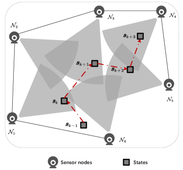
Figure 1: The figure shows a topology with $6$ sensor nodes $\{\mathcal{N}_{1},\mathcal{N}_{2},\dots,\mathcal{N}_{6}\}$. The black solid lines represent the communication links between different nodes. Let the initial state of the object be $\bm{s}_{k-1}$, and then the object has four states $\{\bm{s}_{k},\bm{s}_{k+1},\bm{s}_{k+2},\bm{s}_{k+3}\}$ over time. The figure also shows the existence of “naive” nodes. For example, when the object is in the state $\bm{s}_{k}$, only the node $\mathcal{N}_{1}$ observes the object. The nodes $\{\mathcal{N}_{3},\mathcal{N}_{4},\mathcal{N}_{5}\}$ and their immediate neighboring nodes do not observe the object. Therefore, the nodes $\{\mathcal{N}_{3},\mathcal{N}_{4},\mathcal{N}_{5}\}$ are the “naive” nodes for the state $\bm{s}_{k}$.

Next, we propose a novel state-space model, namely coupled velocity model (CVM), where the correlation between the velocity and orientation is established via a sideslip angle.
(1) State Parameterization

At time $k$, the kinematic state $\bm{x}_{k}$

$$\bm{x}_{k}=[(\bm{x}_{k}^{\mathrm{c}})^{\mathsf{T}},v_{k}^{\mathsf{x}},v_{k}^{\mathsf{y}},\cdots]^{\mathsf{T}}$$ (1)

involves the centroid position $\bm{x}_{k}^{\mathrm{c}}\in\mathbb{R}^{2}$, the velocity $\bm{[}v_{k}^{\mathsf{x}},v_{k}^{\mathsf{y}}]^{\mathsf{T}}:=\bm{\vartheta}_{k}$ in $x$ and $y$ axes, and possible quantities such as acceleration. As for the extent

$$\bm{p}_{k}=[l_{k,1},l_{k,2},\beta_{k}]^{\mathsf{T}},$$ (2)

it involves the semi-lengths $l_{k,1}$ and $l_{k,2}$, and the sideslip angle $\beta_{k}=\arctan(\frac{v_{k}^{\mathsf{y}}}{v_{k}^{\mathsf{x}}})-\alpha_{k}$ that represents a drift between the orientation $\alpha_{k}$ and velocity direction $\arctan(\frac{v_{k}^{\mathsf{y}}}{v_{k}^{\mathsf{x}}})$.
(2) Measurement Model

At time $k$, the measurement $\bm{y}_{k,s}^{i}$ on node $s\in\mathcal{N}$ is given in (3),

$$\bm{y}_{k,s}^{i}=\mathbf{H}\bm{x}_{k}+\underbrace{\begin{bmatrix}\frac{v_{k}^{\mathsf{y}}\sin{\beta_{k}}+v_{k}^{\mathsf{x}}\cos{\beta_{k}}}{\|\bm{\vartheta}_{k}\|}&\frac{{\color[rgb]{1,0,0}v_{k}^{\mathsf{x}}\sin{\beta_{k}}-v_{k}^{\mathsf{y}}\cos{\beta_{k}}}}{\|\bm{\vartheta}_{k}\|}\\ \frac{v_{k}^{\mathsf{y}}\cos{\beta_{k}}-v_{k}^{\mathsf{x}}\sin{\beta_{k}}}{\|\bm{\vartheta}_{k}\|}&\frac{v_{k}^{\mathsf{y}}\sin{\beta_{k}}+v_{k}^{\mathsf{x}}\cos{\beta_{k}}}{\|\bm{\vartheta}_{k}\|}\end{bmatrix}\begin{bmatrix}l_{k,1}&0\\ 0&l_{k,2}\end{bmatrix}}_{:=\mathbf{S}_{k}}\underbrace{{\begin{bmatrix}{h_{k,1}^{i}}\\ {h_{k,2}^{i}}\end{bmatrix}}}_{:=\bm{h}_{k}^{i}}+\bm{v}_{k,s}^{i},$$ (3)

where the measurement matrix $\mathbf{H}=\left[\mathbf{I}_{2}\;\bm{0}\right]$ extracts the position component from $\bm{x}_{k}$, the coefficient matrix $\mathbf{S}_{k}$ compacts the kinematics and extent, and the multiplicative noise $\bm{h}_{k,s}^{i}$ enables any scattering source lying on the boundary or interior of the object. It is assumed that $\bm{v}_{k,1}^{i},\bm{v}_{k,2}^{i},\cdots$ are uncorrelated zero-mean Gaussian noises with covariances $\mathbf{C}_{s}^{v}\delta_{sj}$ if $s=j$, $\delta_{sj}=1$, and $\delta_{sj}=0$, otherwise. Fig. 2 gives an illustration for the model (3).

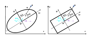
Figure 2: Illustration of the measurement model. The time index $k$, measurement index ${i}$, and sensor node index $s$ are omitted in the figure. The centroid position of the object is $\bm{x}^{\mathrm{c}}$, and its extent and velocity are denoted as $\bm{p}=[l_{1},l_{2},\beta]^{\mathsf{T}}$ and $\bm{\vartheta}=\bm{[}v^{\mathsf{x}},v^{\mathsf{y}}]^{\mathsf{T}}$, respectively. By counterclockwise rotating an angle $\alpha=\arctan({v^{\mathsf{y}}}/{v^{\mathsf{x}}})-\beta$ (i.e., the orientation) along $x$-axis, a reference coordinates $x_{r}$-$y_{r}$ is obtained. The scattering source $\bm{z}$ is compacted by the parameters $\bm{p}$, $\bm{x}^{\mathrm{c}}$ and multiplicative noise $\bm{h}=[h_{1},h_{2}]^{\mathsf{T}}$. The measurement $\bm{y}$ is obtained by the source $\bm{z}$ plus a Gaussian measurement noise $\bm{v}$. The illustration gives a direct view about the correlation between the velocity and orientation. It can be seen that the model is feasible to describe the perpendicular axis-symmetric extents, such as an ellipse or a rectangle.

(3) Dynamic Models

The dynamic models for the kinematics and extent are given as follows:

$$\bm{x}_{k+1}=\mathbf{\Phi}_{k}^{x}\bm{x}_{k}+\bm{w}_{k}^{x}$$ (4)

$$\bm{p}_{k+1}=\mathbf{\Phi}_{k}^{p}\bm{p}_{k}+\bm{w}_{k}^{p}$$ (5)

where $\mathbf{\Phi}_{k}^{x}$ and $\mathbf{\Phi}_{k}^{p}$ are transition matrices, and $\bm{w}_{k}^{x}$ and $\bm{w}_{k}^{p}$ are zero-mean Gaussian process noises with covariances $\mathbf{C}_{w}^{x}$ and $\mathbf{C}_{w}^{p}$, respectively. One can select the corresponding transition matrices according to the actual motion pattern and body structure, e.g., for a rigid object with nearly constant velocity,

$$\mathbf{\Phi}_{k}^{x}=\begin{bmatrix}1&0&\mathrm{T}&0\\ 0&1&0&\mathrm{T}\\ 0&0&1&0\\ 0&0&0&1\end{bmatrix},\qquad\mathbf{\Phi}_{k}^{p}=\mathbf{I}_{3}.$$

Remark 1

• Compared with the previous model in [14], (3) uses the sideslip angle $\beta_{k}$ to establish a tight relation between the velocity components $\bm{[}v_{k}^{\mathsf{x}}\;v_{k}^{\mathsf{y}}]$ and orientation $\alpha_{k}$ from the kinematic perspective. On the one hand, the relation contributes to finding the mismatch between the actual motion pattern and prior dynamic model. A main reason is that the orientation provides an intuitive insight to point out whether the motion pattern has changed. Once the pattern has changed, the corresponding filter should set more weight to the measurement instead of the prior. On the other hand, the relation is capable of describing the object drift cases such as in maritime radar applications [30, 31].

• The dynamic model (5) w.r.t the extent involves the process noise $\bm{w}_{k}^{p}$. Although the study focuses on a rigid object (i.e., its extent is time-invariant), there may exist a distortion of extent to some extent in a sensor’s FoV during the tracking process. Thus, the noise $\bm{w}_{k}^{p}$ is introduced to describe the distortion.

Although the state-space model is given, directly using the model to achieve a centralized or distributed filter still confronts some intractable difficulties. For the centralized filter, a main difficulty is how to process the massive measurements from multiple nodes especially in the EOT scenario. The distributed filter over a network with “naive” nodes faces two difficulties: 1) how to properly balance the weight between the priors and measurements to give a consensus estimate; 2) how to preserve the cross-covariances among the nodes in a distributed tracking system, especially for a large-scale network, so that the distributed estimate closes to the corresponding centralized value (i.e., the optimal estimate) as much as possible.

III Separation of measurement model with coupled kinematics and extent

This study introduces the WLS criterion to handle those aforementioned difficulties. On the one hand, the criterion facilitates the centralized filter to reduce its computational cost by converting the massive data into a compact summation form. On the other hand, it allows the local estimate on each node to be given a proper weight in the final result. However, it requires a linear state-space model with only additive noise about the estimated state. Thus, we separate (3) into two pseudo-linearized models to satisfy the requirement.

Here, the measurements $\{\bm{y}_{k,s}^{i}\}^{n_{k,s}}_{i=1}$ on node $s\in\mathcal{N}$ are processed sequentially. Let $\hat{\bm{x}}_{k}^{[i-1]}$, $\hat{\bm{p}}_{k}^{[i-1]}$, $\mathbf{C}_{k}^{x[i-1]}$ and $\mathbf{C}_{k}^{p[i-1]}$ denote the prior estimates for the kinematics $\bm{x}_{k}$ and extent $\bm{p}_{k}$ plus their corresponding covariances at the ${[i-1]}$-th sequential operation. The node $s$ processes $\bm{y}_{k,s}^{i}$ to obtain the updated estimates $\hat{\bm{x}}_{k}^{[i]}$, $\hat{\bm{p}}_{k}^{[i]}$, $\mathbf{C}_{k}^{x[i]}$ and $\mathbf{C}_{k}^{p[i]}$. Next, we focus on presenting two pseudo-linearized measurement models w.r.t $\bm{x}_{k}$ and $\bm{p}_{k}$, respectively.

Proposition 1 (Separate model I)

The measurement model about $\bm{x}_{k}$ is

$$\bm{y}_{k,s}^{i}\approx\mathbf{H}\bm{x}_{k}+\bm{v}_{k,s}^{x[i]},$$ (6)

where $\bm{v}_{k}^{x[i]}$ is the equivalent noise with $\mathbb{E}(\bm{v}_{k,s}^{x[i]})=\bm{0}$, $\mathrm{Cov}(\bm{v}_{k,s}^{x[i]})=\mathbf{R}_{k,s}^{x[i]}:=\mathbf{C}^{\mathrm{\@slowromancap i@}}+\mathbf{C}^{\mathrm{\@slowromancap ii@}}+\mathbf{C}^{\mathrm{\@slowromancap iii@}}+\mathbf{C}_{s}^{v}$. The terms $\mathbf{C}^{\mathrm{\@slowromancap i@}}$, $\mathbf{C}^{\mathrm{\@slowromancap ii@}}$, and $\mathbf{C}^{\mathrm{\@slowromancap iii@}}$ are given as follows:

$$\mathbf{C}^{\mathrm{\@slowromancap i@}}=\hat{\mathbf{S}}_{k}^{[i-1]}\mathbf{C}^{h}\left(\hat{\mathbf{S}}_{k}^{[i-1]}\right)^{\mathsf{T}},$$ (7)

$$\underbrace{[\epsilon_{mn}]}_{\mathbf{C}^{\mathrm{\@slowromancap ii@}}}=\mathrm{tr}\left\{\mathbf{C}_{k}^{p[i-1]}\left(\hat{\mathbf{J}}_{nk,p}^{[i-1]}\right)^{\mathsf{T}}\mathbf{C}^{h}\hat{\mathbf{J}}_{mk,p}^{[i-1]}\right\},$$ (8)

$$\underbrace{[\varpi_{mn}]}_{\mathbf{C}^{\mathrm{\@slowromancap iii@}}}=\mathrm{tr}\left\{\mathbf{H}\mathbf{C}_{k}^{x[i-1]}\mathbf{H}^{\mathsf{T}}\left(\hat{\mathbf{J}}_{nk,v}^{[i-1]}\right)^{\mathsf{T}}\mathbf{C}^{h}\hat{\mathbf{J}}_{mk,v}^{[i-1]}\right\},$$ (9)

for $m,n\in\{1,2\}$. The intermediate quantities $\hat{\mathbf{J}}_{1k,p}^{[i-1]}$, $\hat{\mathbf{J}}_{2k,p}^{[i-1]}$, $\hat{\mathbf{J}}_{1k,v}^{[i-1]}$, and $\hat{\mathbf{J}}_{2k,v}^{[i-1]}$ are the Jacobian matrices of the first row $\mathbf{S}_{1,k}$ and second row $\mathbf{S}_{2,k}$ of $\mathbf{S}_{k}$ around the ${[i-1]}$-th extent estimate $\hat{\bm{p}}_{k}^{[i-1]}$ and velocity estimate $\hat{\bm{\vartheta}}_{k}^{[i-1]}$, respectively.

Proof:

See Appendix A. ∎

Notice that the quantities $\mathbf{C}^{\mathrm{\@slowromancap i@}}$, $\mathbf{C}^{\mathrm{\@slowromancap ii@}}$, and $\mathbf{C}^{\mathrm{\@slowromancap iii@}}$ in (6) are treated as constant terms at the $[i]$-th sequential operation since they are calculated based on the former estimates $\hat{\bm{p}}_{k}^{[i-1]}$ and $\hat{\bm{\vartheta}}_{k}^{[i-1]}$.

Due to the existence of zero-mean multiplicative noise $\bm{h}_{k}^{i}$, a pseudo-measurement using 2-fold Kronecker product is required to update the extent [14, 32]. The ${[i]}$-th pseudo-measurement $\mathbf{Y}_{k}^{[i]}$ is given as

$$\mathbf{Y}_{k,s}^{[i]}=\mathbf{F}\left((\bm{y}_{k,s}^{i}-\mathbf{H}\hat{\bm{x}}_{k}^{[i-1]})\otimes(\bm{y}_{k,s}^{i}-\mathbf{H}\hat{\bm{x}}_{k}^{[i-1]})\right),$$ (10)

and its expectation is

$$\mathbb{E}(\mathbf{Y}_{k,s}^{[i]})=\mathbf{F}\mathrm{vect}\left(\mathbf{C}_{k,s}^{y[i]}\right),$$ (11)

residual covariance is

$$\mathrm{Cov}(\mathbf{Y}_{k,s}^{[i]})=\mathbf{F}\left(\mathbf{C}_{k,s}^{y[i]}\otimes\mathbf{C}_{k,s}^{y[i]}\right)(\mathbf{F}+\tilde{\mathbf{F}})^{\mathsf{T}}$$ (12)

with

$$\mathbf{F}=\begin{bmatrix}1&0&0&0\\ 0&0&0&1\\ 0&1&0&0\end{bmatrix},\quad\tilde{\mathbf{F}}=\begin{bmatrix}1&0&0&0\\ 0&0&0&1\\ 0&0&1&0\end{bmatrix}.$$ (13)

Proposition 2 (Separate model II)

According to (10), the measurement model about $\bm{p}_{k}$ is

$$\mathbf{Y}_{k,s}^{[i]}\approx\hat{\mathbf{M}}_{k}^{[i-1]}\bm{p}_{k}+\bm{v}_{k,s}^{p[i]}$$ (14)

where

$$\hat{\mathbf{M}}_{k}^{[i-1]}=\begin{bmatrix}2\hat{\mathbf{S}}_{1,k}^{[i-1]}\mathbf{C}^{h}\hat{\mathbf{J}}_{1k,p}^{[i-1]}\\ 2\hat{\mathbf{S}}_{2,k}^{[i-1]}\mathbf{C}^{h}\hat{\mathbf{J}}_{2k,p}^{[i-1]}\\ \hat{\mathbf{S}}_{1,k}^{[i-1]}\mathbf{C}^{h}\hat{\mathbf{J}}_{2k,p}^{[i-1]}+\hat{\mathbf{S}}_{2,k}^{[i-1]}\mathbf{C}^{h}\hat{\mathbf{J}}_{1k,p}^{[i-1]}\end{bmatrix},$$ (15)

and $\bm{v}_{k,s}^{p[i]}$ is the equivalent noise with

$$\mathbb{E}(\bm{v}_{k,s}^{p[i]})=\bar{\bm{v}}_{k,s}^{p[i]}:=\mathbf{F}\mathrm{vect}\left(\mathbf{C}_{k,s}^{y[i]}\right)-\hat{\mathbf{M}}_{k}^{[i-1]}\hat{\bm{p}}_{k}^{[i-1]},$$ (16)

$$\begin{split}\mathrm{Cov}(\bm{v}_{k,s}^{p[i]})=\mathbf{R}_{k,s}^{p[i]}:=&\mathbf{F}\left(\mathbf{C}_{k,s}^{y[i]}\otimes\mathbf{C}_{k,s}^{y[i]}\right)(\mathbf{F}+\tilde{\mathbf{F}})^{\mathsf{T}}\\ &-\hat{\mathbf{M}}_{k}^{[i-1]}\mathbf{C}_{k}^{p[i-1]}\hat{\mathbf{M}}_{k}^{[i-1]{\mathsf{T}}}.\end{split}$$ (17)

Proof:

See Appendix B. ∎

Remark 2

• Although the models (6) and (14) are separated from (3), the interdependency between the kinematics $\bm{x}_{k}$ and extent $\bm{p}_{k}$ still remains as parameters in each other’s model. In this condition, the joint estimation of $\bm{x}_{k}$ and $\bm{p}_{k}$ is transferred into an iterative operation of related linear filters.

• Considering the complex calculation in the higher-order terms, such as the Hessian matrix, the models (6) and (14) only utilize the first-order Taylor series expansion in (47). Moreover, the model (14) merely depends on (47) as an essential prerequisite, otherwise (14) cannot be obtained.

IV Centralized WLS Filter

This section presents a centralized weighted least squares filter (CWLSF) as a benchmark for the following distributed filter. The CWLSF first integrates the models (6) and (14) into the WLS structure, and then the estimated states are alternately updated in two linear filters.

IV-A Measurement Update

In the measurement update, the accumulated measurements $\mathcal{Y}_{k}=\{\mathcal{Y}_{k,s}\}_{s\in\mathcal{N}}$ from all nodes are gathered into the fusion center. For clarity, assume that there are $n_{k}$ measurements at time $k$ for each node $s\in\mathcal{N}$. Given the $[i-1]$-th prior estimates, the fusion center sequentially processes $\{\bm{y}_{k,s}^{i}\}_{s\in\mathcal{N}}$ to give the updated estimates. According to (6), define the central measurement, measurement matrix, noise covariance, and noise information matrix related to the measurement set $\{\bm{y}_{k,s}^{i}\}_{s\in\mathcal{N}}$ as

$$\left\{\begin{lgathered}\bm{y}_{k,\mathrm{c}}^{i}:=\mathrm{col}(\bm{y}_{k,1}^{i},\bm{y}_{k,2}^{i},\cdots,\bm{y}_{k,\lvert\mathcal{N}\rvert}^{i});\;\mathbf{H}_{\mathrm{c}}:=[\mathbf{H};\mathbf{H};\cdots;\mathbf{H}]\\ \bm{\nu}_{k,\mathrm{c}}^{x{[i]}}:=\mathrm{col}(\bm{v}_{k,1}^{x{[i]}},\bm{\nu}_{k,2}^{x{[i]}},\cdots,\bm{v}_{k,\lvert\mathcal{N}\rvert}^{x{[i]}})\\ \mathbf{R}_{k,\mathrm{c}}^{x[i]}:=\mathrm{diag}(\mathbf{R}_{k,1}^{x[i]},\mathbf{R}_{k,2}^{x[i]},\cdots,\mathbf{R}_{k,\lvert\mathcal{N}\rvert}^{x[i]})\\ \mathbf{V}_{k,\mathrm{c}}^{x[i]}:=\mathrm{diag}(\mathbf{V}_{k,1}^{x[i]},\dots,\mathbf{V}_{k,\lvert\mathcal{N}\rvert}^{x[i]})=(\mathbf{R}_{k,\mathrm{c}}^{x[i]})^{-1}\end{lgathered}\bm{y}_{k,\mathrm{c}}^{i}:=\mathrm{col}(\bm{y}_{k,1}^{i},\bm{y}_{k,2}^{i},\cdots,\bm{y}_{k,\lvert\mathcal{N}\rvert}^{i});\;\mathbf{H}_{\mathrm{c}}:=[\mathbf{H};\mathbf{H};\cdots;\mathbf{H}]\\ \bm{\nu}_{k,\mathrm{c}}^{x{[i]}}:=\mathrm{col}(\bm{v}_{k,1}^{x{[i]}},\bm{\nu}_{k,2}^{x{[i]}},\cdots,\bm{v}_{k,\lvert\mathcal{N}\rvert}^{x{[i]}})\\ \mathbf{R}_{k,\mathrm{c}}^{x[i]}:=\mathrm{diag}(\mathbf{R}_{k,1}^{x[i]},\mathbf{R}_{k,2}^{x[i]},\cdots,\mathbf{R}_{k,\lvert\mathcal{N}\rvert}^{x[i]})\\ \mathbf{V}_{k,\mathrm{c}}^{x[i]}:=\mathrm{diag}(\mathbf{V}_{k,1}^{x[i]},\dots,\mathbf{V}_{k,\lvert\mathcal{N}\rvert}^{x[i]})=(\mathbf{R}_{k,\mathrm{c}}^{x[i]})^{-1}\right.$$ (18)

where the subscript “c” denotes “central”, and $\lvert\mathcal{N}\rvert$ is the cardinality of $\mathcal{N}$. If a node $s$ does not obtain measurements, let $\bm{y}_{k,s}^{i}=\bm{0}$, $\mathbf{V}_{k,s}^{x[i]}=\bm{0}$.

According to (14), define the central measurement, measurement matrix, noise covariance, and noise information matrix related to the pseudo-measurement set $\{{\mathbf{Y}}_{k,s}^{[i]}\}_{s\in\mathcal{N}}$ as

$$\left\{\begin{lgathered}\tilde{\mathbf{Y}}_{k,s}^{[i]}:=\mathbf{Y}_{k,s}^{[i]}-\bar{\bm{v}}_{k,s}^{p{[i]}},\>\tilde{\bm{v}}_{k,s}^{p{[i]}}:=\bm{v}_{k,s}^{p{[i]}}-\bar{\bm{v}}_{k,s}^{p{[i]}}\\ \tilde{\mathbf{Y}}_{k,\mathrm{c}}^{[i]}:=\mathrm{col}(\tilde{\mathbf{Y}}_{k,1}^{[i]},\tilde{\mathbf{Y}}_{k,2}^{[i]},\cdots,\tilde{\mathbf{Y}}_{k,\lvert\mathcal{N}\rvert}^{[i]})\\ \mathbf{M}_{k,\mathrm{c}}^{[i-1]}:=[\hat{\mathbf{M}}_{k}^{[i-1]};\hat{\mathbf{M}}_{k}^{[i-1]};\cdots;\hat{\mathbf{M}}_{k}^{[i-1]}]\\ \bm{\nu}_{k,\mathrm{c}}^{p{[i]}}:=\mathrm{col}(\tilde{\bm{v}}_{k,1}^{p{[i]}},\tilde{\bm{v}}_{k,2}^{p{[i]}},\cdots,\tilde{\bm{v}}_{k,\lvert\mathcal{N}\rvert}^{p{[i]}})\\ \mathbf{R}_{k,\mathrm{c}}^{p[i]}=\mathrm{diag}(\mathbf{R}_{k,1}^{p[i]},\mathbf{R}_{k,2}^{p[i]},\cdots,\mathbf{R}_{k,\lvert\mathcal{N}\rvert}^{p[i]})\\ \mathbf{V}_{k,\mathrm{c}}^{p[i]}:=\mathrm{diag}(\mathbf{V}_{k,1}^{p[i]},\ldots,\mathbf{V}_{k,\lvert\mathcal{N}\rvert}^{p[i]})=(\mathbf{R}_{k,\mathrm{c}}^{p[i]})^{-1}\end{lgathered}\tilde{\mathbf{Y}}_{k,s}^{[i]}:=\mathbf{Y}_{k,s}^{[i]}-\bar{\bm{v}}_{k,s}^{p{[i]}},\>\tilde{\bm{v}}_{k,s}^{p{[i]}}:=\bm{v}_{k,s}^{p{[i]}}-\bar{\bm{v}}_{k,s}^{p{[i]}}\\ \tilde{\mathbf{Y}}_{k,\mathrm{c}}^{[i]}:=\mathrm{col}(\tilde{\mathbf{Y}}_{k,1}^{[i]},\tilde{\mathbf{Y}}_{k,2}^{[i]},\cdots,\tilde{\mathbf{Y}}_{k,\lvert\mathcal{N}\rvert}^{[i]})\\ \mathbf{M}_{k,\mathrm{c}}^{[i-1]}:=[\hat{\mathbf{M}}_{k}^{[i-1]};\hat{\mathbf{M}}_{k}^{[i-1]};\cdots;\hat{\mathbf{M}}_{k}^{[i-1]}]\\ \bm{\nu}_{k,\mathrm{c}}^{p{[i]}}:=\mathrm{col}(\tilde{\bm{v}}_{k,1}^{p{[i]}},\tilde{\bm{v}}_{k,2}^{p{[i]}},\cdots,\tilde{\bm{v}}_{k,\lvert\mathcal{N}\rvert}^{p{[i]}})\\ \mathbf{R}_{k,\mathrm{c}}^{p[i]}=\mathrm{diag}(\mathbf{R}_{k,1}^{p[i]},\mathbf{R}_{k,2}^{p[i]},\cdots,\mathbf{R}_{k,\lvert\mathcal{N}\rvert}^{p[i]})\\ \mathbf{V}_{k,\mathrm{c}}^{p[i]}:=\mathrm{diag}(\mathbf{V}_{k,1}^{p[i]},\ldots,\mathbf{V}_{k,\lvert\mathcal{N}\rvert}^{p[i]})=(\mathbf{R}_{k,\mathrm{c}}^{p[i]})^{-1}\right..$$ (19)

If a node $s$ does not obtain measurements, let $\tilde{\mathbf{Y}}_{k,s}^{[i]}=\bm{0}$, $\mathbf{V}_{k,s}^{p[i]}=\bm{0}$.

Define

• the prior error of kinematics ${\bm{x}}_{k}$ as $\tilde{\bm{x}}_{k}^{[i-1]}:=\hat{\bm{x}}^{[i-1]}_{k}-{\bm{x}}_{k}$,

• the corresponding covariance as $\mathrm{Cov}(\tilde{\bm{x}}_{k}^{[i-1]}):=\mathbf{C}^{x[i-1]}_{k}$,

• the information matrix as $\mathbf{\Omega}^{x[i-1]}_{k}:=\left(\mathbf{C}_{k}^{x[i-1]}\right)^{-1}$.

Similarly, define

• the prior error of extent ${\bm{p}}_{k}$ as $\tilde{\bm{p}}_{k}^{[i-1]}:=\hat{\bm{p}}^{[i-1]}_{k}-{\bm{p}}_{k}$,

• the corresponding covariance as $\mathrm{Cov}(\tilde{\bm{p}}_{k}^{[i-1]}):=\mathbf{C}^{p[i-1]}_{k}$,

• the information matrix as $\mathbf{\Omega}^{p[i-1]}_{k}:=\left(\mathbf{C}_{k}^{p[i-1]}\right)^{-1}$.

Here, the notation $(\cdot)_{k}^{[0]}$ denotes the predicted estimate at time $k$.

Combining (18) with prior error $\tilde{\bm{x}}_{k}^{[i-1]}$ yields

$$\begin{bmatrix}\hat{\bm{x}}^{[i-1]}_{k}\\ \bm{y}_{k,\mathrm{c}}^{i}\end{bmatrix}=\begin{bmatrix}\mathbf{I}\\ \mathbf{H}_{\mathrm{c}}\end{bmatrix}\bm{x}_{k}+\begin{bmatrix}\tilde{\bm{x}}_{k}^{[i-1]}\\ \bm{\nu}_{k,c}^{x{[i]}}\end{bmatrix}.$$ (20)

The centralized WLS estimate of the kinematics $\bm{x}_{k}$ plus information matrix are

$$\begin{split}\hat{\bm{x}}^{[i]}_{k}=&\left(\mathbf{\Omega}^{x[i-1]}_{k}+\sum_{s\in\mathcal{N}}\mathbf{H}^{\mathsf{T}}\mathbf{V}_{k,s}^{x[i]}\mathbf{H}\right)^{-1}\\ &\times\left(\mathbf{\Omega}^{x[i-1]}_{k}\hat{\bm{x}}^{[i-1]}_{k}+\sum_{s\in\mathcal{N}}\mathbf{H}^{\mathsf{T}}\mathbf{V}_{k,s}^{x[i]}\bm{y}_{k,s}^{i}\right),\end{split}$$ (21a)

$$\mathbf{\Omega}^{x[i]}_{k}=\mathbf{\Omega}^{x[i-1]}_{k}+\sum_{s\in\mathcal{N}}\mathbf{H}^{\mathsf{T}}\mathbf{V}_{k,s}^{x[i]}\mathbf{H}.$$ (21b)

Also, combining (19) with prior error $\tilde{\bm{p}}_{k}^{[i-1]}$ yields

$$\begin{bmatrix}\hat{\bm{p}}^{[i-1]}_{k}\\ \tilde{\mathbf{Y}}_{k,\mathrm{c}}^{[i]}\end{bmatrix}=\begin{bmatrix}\mathbf{I}\\ \mathbf{M}_{k,\mathrm{c}}^{[i-1]}\end{bmatrix}\bm{p}_{k}+\begin{bmatrix}\tilde{\bm{p}}_{k}^{[i-1]}\\ \bm{\nu}_{k,c}^{p{[i]}}\end{bmatrix}.$$ (22)

The centralized WLS estimate of the extent $\bm{p}_{k}$ plus information matrix are

$$\begin{split}\hat{\bm{p}}^{[i]}_{k}=&\left(\mathbf{\Omega}^{p[i-1]}_{k}+\sum_{s\in\mathcal{N}}\left(\hat{\mathbf{M}}_{k}^{[i-1]}\right)^{\mathsf{T}}\mathbf{V}_{k,s}^{p[i]}\hat{\mathbf{M}}_{k}^{[i-1]}\right)^{-1}\\ &\times\left(\mathbf{\Omega}^{p[i-1]}_{k}\hat{\bm{p}}^{[i-1]}_{k}+\left(\hat{\mathbf{M}}_{k}^{[i-1]}\right)^{\mathsf{T}}\mathbf{V}_{k,s}^{p[i]}\tilde{\mathbf{Y}}_{k,s}^{[i]}\right),\end{split}$$ (23a)

$$\mathbf{\Omega}^{p[i]}_{k}=\mathbf{\Omega}^{p[i-1]}_{k}+\sum_{s\in\mathcal{N}}\left(\hat{\mathbf{M}}_{k}^{[i-1]}\right)^{\mathsf{T}}\mathbf{V}_{k,s}^{p[i]}\hat{\mathbf{M}}_{k}^{[i-1]}.$$ (23b)

Notice that the measurements from all nodes are processed via a summation form as shown in (21a) and (23a), which overcomes the data congestion in the centralized system to some extent.

IV-B Time Update

After the $n_{k}$ batch of measurements are processed sequentially, (24) and (25) are performed to accomplish the time update. Since the temporal evolutions of both the kinematics and extent follow a linear model, the predicted estimates have the same form as in the information filter [34], i.e.,

$$\hat{\bm{x}}^{[0]}_{k+1}=\mathbf{\Phi}_{k}^{x}\hat{\bm{x}}^{[n_{k}]}_{k},$$ (24a)

$$\mathbf{\Omega}_{k+1}^{x[0]}=\left(\mathbf{\Phi}_{k}^{x}\left(\mathbf{\Omega}_{k}^{x[n_{k}]}\right)^{-1}\left(\mathbf{\Phi}_{k}^{x}\right)^{\mathsf{T}}+\mathbf{C}_{w}^{x}\right)^{-1},$$ (24b)

$$\hat{\bm{p}}^{[0]}_{k+1}=\mathbf{\Phi}_{k}^{p}\hat{\bm{p}}^{[n_{k}]}_{k},$$ (25a)

$$\mathbf{\Omega}_{k+1}^{p[0]}=\left(\mathbf{\Phi}_{k}^{p}\left(\mathbf{\Omega}_{k}^{p[n_{k}]}\right)^{-1}\left(\mathbf{\Phi}_{k}^{p}\right)^{\mathsf{T}}+\mathbf{C}_{w}^{p}\right)^{-1}.$$ (25b)

1 Initialization: $\hat{\bm{x}}_{1}^{[0]}$, $\hat{\bm{p}}_{1}^{[0]}$, $\mathbf{\Omega}_{1}^{x[0]}$, and $\mathbf{\Omega}_{1}^{p[0]}$ ;

2 for $k\leftarrow 1,2,\cdots$ // scan time  do

3       Data: $\{\bm{y}_{k,s}^{i}\}^{n_{k}}_{i=1}(s\in\mathcal{N})$ ;

4       Initialization: $\hat{\bm{x}}_{k}^{[0]}$, $\hat{\bm{p}}_{k}^{[0]}$, $\mathbf{\Omega}_{k}^{x[0]}$, and $\mathbf{\Omega}_{k}^{p[0]}$ ;

5      

6      for $i=1,2,\cdots,n_{k}$ // sequential  do

7            compute $\hat{\bm{x}}_{k}^{[i]},\mathbf{\Omega}_{k}^{x[i]},\hat{\bm{p}}_{k}^{[i]},\mathbf{\Omega}_{k}^{p[i]}$ via (21) and (23)

8       end for

9      Output1: $\hat{\bm{x}}_{k}\leftarrow\hat{\bm{x}}_{k}^{[n_{k}]},\mathbf{C}_{k}^{x}\leftarrow\left(\mathbf{\Omega}_{k}^{x[n_{k}]}\right)^{-1}$ ;

10       Output2: $\hat{\bm{p}}_{k}\leftarrow\hat{\bm{p}}_{k}^{[n_{k}]},\mathbf{C}_{k}^{p}\leftarrow\left(\mathbf{\Omega}_{k}^{p[n_{k}]}\right)^{-1}$ ;

11       compute $\hat{\bm{x}}_{k+1}^{[0]},\mathbf{\Omega}_{k+1}^{x[0]},\hat{\bm{p}}_{k+1}^{[0]},\mathbf{\Omega}_{k+1}^{p[0]}$ via (24) and (25)

12 end for

Algorithm 1 CWLSF Filter

The detailed CWLSF is collected in Algorithm 1. It is important to note, that using (6) and (14) to achieve the corresponding filters poses that the interdependency between $\bm{x}_{k}$ and $\bm{p}_{k}$ exists in the $[i]$-th and $[i-1]$-th sequential operation. Here, Fig. 3 gives an illustration of the interdependency in CWLSF.

.

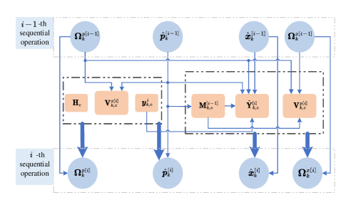
Figure 3: An illustration of the interdependency between $\bm{x}_{k}$ and $\bm{p}_{k}$.

V Distributed WLS Filter

For a distributed system, a primary goal is to make the estimates between nodes achieve consensus. Meanwhile, the estimate on each node converges to the corresponding centralized value. However, due to the naivety and resource constraints, the goal may not be fully achieved at any given time.

Here, we design such a distributed WLS filter (DWLSF). Therein, DWLSF directly operates a consensus on the prior estimate set $\{\hat{\bm{x}}^{[i-1]}_{k,s},\hat{\bm{p}}^{[i-1]}_{k,s}\}_{s\in\mathcal{N}}$ to retain the cross-covariances across all the nodes, and then the updated estimate set $\{\hat{\bm{x}}^{[i]}_{k,s},\hat{\bm{p}}^{[i]}_{k,s}\}_{s\in\mathcal{N}}$ yields an optimal estimates (if the priors are converged to the same value). Next, we just take $\hat{\bm{x}}^{[i-1]}_{k,s}$ for an example to discuss how to achieve this.

Average Consensus (AC) is a popular consensus scheme to compute the arithmetic mean $\frac{1}{\lvert\mathcal{N}\rvert}\sum_{s\in\mathcal{N}}a_{s}$ of a variable set $\{a_{s}\}_{s\in\mathcal{N}}$ [35]. Define the initial value on each node $s\in\mathcal{N}$ be $a_{s}(0)$. At the $l$-th iteration, each node $s$ updates its value using the following protocol

$$a_{s}(l)=a_{s}(l-1)+\xi\sum_{j\in\mathcal{N}^{s}\setminus\{s\}}\left(a_{j}(l-1)-a_{s}(l-1)\right).$$ (26)

By iteratively doing this, the values at all the nodes converge to the average value $\frac{1}{\lvert\mathcal{N}\rvert}\sum_{s\in\mathcal{N}}a_{s}$. The rate parameter $\xi$ is chosen between $0$ and $\frac{1}{\triangle\max}$, where $\triangle\max$ is the maximum degree of the network $\mathcal{G}$.

Suppose that consensus is performed directly on the priors, at the $l$-th iteration, the estimate on node $s$ is described as follows (here, the superscript $[i-1]$ is omitted):

$$\hat{\bm{x}}^{(l)}_{k,s}=\underbrace{\bm{x}_{k}+\tilde{\bm{x}}_{k}}_{\hat{\bm{x}}_{k}}+\bm{\delta}_{k,s}^{x(l)}$$ (27)

where $\bm{\delta}_{k,s}^{x(l)}$ denotes the bias between the local estimate $\hat{\bm{x}}^{(l)}_{k,s}$ and centralized estimate $\hat{\bm{x}}_{k}$, and consensus makes $\bm{\delta}_{k,s}^{x(l)}\to 0$ if the iteration $L$ approaches to $\infty$.

The error covariance in (27) is defined as $\mathbf{C}_{k,ss}^{x(l)}:=\mathbb{E}[\bm{\eta}_{k,s}^{x(l)}(\bm{\eta}_{k,s}^{x(l)})^{\mathsf{T}}]$, where the prior error $\bm{\eta}_{k,s}^{x(l)}=\tilde{\bm{x}}_{k}+\bm{\delta}_{k,s}^{x(l)}$. Similarly, the error cross-covariance for any pair of nodes $\{s,j\}$ is $\mathbf{C}_{k,sj}^{x(l)}:=\mathbb{E}[\bm{\eta}_{k,s}^{x(l)}(\bm{\eta}_{k,j}^{x(l)})^{\mathsf{T}}]$. We drop the iteration index $(l)$, and define the collective prior estimate, prior error, and coefficient matrix as

$$\left\{\begin{lgathered}\bm{\mathcal{X}}_{k,\mathrm{c}}^{[i-1]}:=\left[\left(\hat{\bm{x}}_{k,1}^{[i-1]}\right)^{\mathsf{T}},\left(\hat{\bm{x}}_{k,2}^{[i-1]}\right)^{\mathsf{T}},\cdots,\left(\hat{\bm{x}}_{k,|\mathcal{N}|}^{[i-1]}\right)^{\mathsf{T}}\right]^{\mathsf{T}},\\ \bm{\eta}_{k,\mathrm{c}}^{x[i-1]}:=\left[\left(\bm{\eta}_{k,1}^{x[i-1]}\right)^{\mathsf{T}},\left(\bm{\eta}_{k,2}^{x[i-1]}\right)^{\mathsf{T}},\cdots,\left(\bm{\eta}_{k,|\mathcal{N}|}^{x[i-1]}\right)^{\mathsf{T}}\right]^{\mathsf{T}},\\ \bm{\mathcal{H}}_{I}:=\underbrace{\left[\mathbf{I},\mathbf{I},\cdots,\mathbf{I}\right]^{\mathsf{T}}}_{|\mathcal{N}|}.\end{lgathered}\bm{\mathcal{X}}_{k,\mathrm{c}}^{[i-1]}:=\left[\left(\hat{\bm{x}}_{k,1}^{[i-1]}\right)^{\mathsf{T}},\left(\hat{\bm{x}}_{k,2}^{[i-1]}\right)^{\mathsf{T}},\cdots,\left(\hat{\bm{x}}_{k,|\mathcal{N}|}^{[i-1]}\right)^{\mathsf{T}}\right]^{\mathsf{T}},\\ \bm{\eta}_{k,\mathrm{c}}^{x[i-1]}:=\left[\left(\bm{\eta}_{k,1}^{x[i-1]}\right)^{\mathsf{T}},\left(\bm{\eta}_{k,2}^{x[i-1]}\right)^{\mathsf{T}},\cdots,\left(\bm{\eta}_{k,|\mathcal{N}|}^{x[i-1]}\right)^{\mathsf{T}}\right]^{\mathsf{T}},\\ \bm{\mathcal{H}}_{I}:=\underbrace{\left[\mathbf{I},\mathbf{I},\cdots,\mathbf{I}\right]^{\mathsf{T}}}_{|\mathcal{N}|}.\right.$$ (28)

Combining (18) with (28) yields

$$\begin{bmatrix}\bm{\mathcal{X}}_{k,\mathrm{c}}^{[i-1]}\\ \bm{y}_{k,\mathrm{c}}^{i}\end{bmatrix}=\begin{bmatrix}\bm{\mathcal{H}}_{I}\\ \mathbf{H}_{\mathrm{c}}\end{bmatrix}\bm{x}_{k}+\begin{bmatrix}{\bm{\eta}}_{k,\mathrm{c}}^{x[i-1]}\\ \bm{\nu}_{k,\mathrm{c}}^{x{[i]}}\end{bmatrix}.$$ (29)

Denote the covariance and information matrix of error ${\bm{\eta}}_{k,\mathrm{c}}^{x[i-1]}$, respectively, as follows

$$\mathbf{C}^{x[i-1]}_{k,\mathrm{c}}=\begin{bmatrix}\mathbf{C}^{x[i-1]}_{k,11}&\mathbf{P}^{x[i-1]}_{k,12}&\dots&\mathbf{C}^{x[i-1]}_{k,1|\mathcal{N}|}\\ \mathbf{C}^{x[i-1]}_{k,21}&\mathbf{P}^{x[i-1]}_{k,22}&&\vdots\\ \vdots&&\ddots&\\ \mathbf{C}^{x[i-1]}_{k,|\mathcal{N}|1}&\dots&&\mathbf{C}^{x[i-1]}_{k,|\mathcal{N}||\mathcal{N}|}\end{bmatrix},$$ (30)

$$\mathbf{F}^{x[i-1]}_{k,\mathrm{c}}=\begin{bmatrix}\mathbf{F}^{x[i-1]}_{k,11}&\mathbf{F}^{x[i-1]}_{k,12}&\dots&\mathbf{F}^{x[i-1]}_{k,1|\mathcal{N}|}\\ \mathbf{F}^{x[i-1]}_{k,21}&\mathbf{F}^{x[i-1]}_{k,22}&&\vdots\\ \vdots&&\ddots&\\ \mathbf{F}^{x[i-1]}_{k,|\mathcal{N}|1}&\dots&&\mathbf{F}^{x[i-1]}_{k,|\mathcal{N}||\mathcal{N}|}\end{bmatrix}.$$ (31)

From (29) and (31), the centralized WLS estimate of the kinematics $\bm{x}_{k}$ and information matrix are given as

$$\begin{split}\hat{\bm{x}}^{[i]}_{k}=&{}\left(\bm{\mathcal{H}}_{I}^{\mathsf{T}}\mathbf{F}^{x[i-1]}_{k,\mathrm{c}}\bm{\mathcal{H}}_{I}+\left(\mathbf{H}_{\mathrm{c}}\right)^{\mathsf{T}}\mathbf{V}_{k,\mathrm{c}}^{x[i]}\mathbf{H}_{\mathrm{c}}\right)^{-1}\\ &\mathrel{\phantom{=}}{}\times\left(\bm{\mathcal{H}}_{I}^{\mathsf{T}}\mathbf{F}^{x[i-1]}_{k,\mathrm{c}}\bm{\mathcal{X}}_{k,\mathrm{c}}^{[i-1]}+\left(\mathbf{H}_{\mathrm{c}}\right)^{\mathsf{T}}\mathbf{V}_{k,\mathrm{c}}^{x[i]}\bm{y}_{k,\mathrm{c}}^{i}\right)\\ =&{}\left(\sum_{s\in\mathcal{N}}(\mathbf{F}^{x[i-1]}_{k,s}+\mathbf{U}^{x[i]}_{k,s})\right)^{-1}\!\sum_{s\in\mathcal{N}}(\mathbf{F}^{x[i-1]}_{k,s}\hat{\bm{x}}_{k,s}^{[i-1]}+\bm{u}^{x[i]}_{k,s}),\end{split}$$ (32)

$$\mathbf{\Omega}^{x[i]}_{k}=\sum_{s\in\mathcal{N}}\left(\mathbf{F}^{x[i-1]}_{k,s}+\mathbf{U}^{x[i]}_{k,s}\right),$$ (33)

where

$$\left\{\begin{lgathered}\mathbf{F}^{x[i-1]}_{k,s}=\sum_{j\in\mathcal{N}}\mathbf{F}^{x[i-1]}_{k,js},\quad\mathbf{U}^{x[i]}_{k,s}=\mathbf{H}^{\mathsf{T}}\mathbf{V}_{k,s}^{x[i]}\mathbf{H},\\ \bm{u}^{x[i]}_{k,s}=\mathbf{H}^{\mathsf{T}}\mathbf{V}_{k,s}^{x[i]}\bm{y}_{k,s}^{i}.\end{lgathered}\mathbf{F}^{x[i-1]}_{k,s}=\sum_{j\in\mathcal{N}}\mathbf{F}^{x[i-1]}_{k,js},\quad\mathbf{U}^{x[i]}_{k,s}=\mathbf{H}^{\mathsf{T}}\mathbf{V}_{k,s}^{x[i]}\mathbf{H},\\ \bm{u}^{x[i]}_{k,s}=\mathbf{H}^{\mathsf{T}}\mathbf{V}_{k,s}^{x[i]}\bm{y}_{k,s}^{i}.\right.$$ (34)

In an analogous definitions about the kinematics in (28) to (31), the centralized WLS estimate of the extent $\bm{p}_{k}$ and information matrix are given as

$$\hat{\bm{p}}^{[i]}_{k}=\left(\sum_{s\in\mathcal{N}}(\mathbf{F}^{p[i-1]}_{k,s}+\mathbf{U}^{p[i]}_{k,s})\right)^{-1}\sum_{s\in\mathcal{N}}(\mathbf{F}^{p[i-1]}_{k,s}\hat{\bm{p}}_{k,s}^{[i-1]}+\bm{u}^{p[i]}_{k,s}),$$ (35)

$$\mathbf{\Omega}^{p[i]}_{k}=\sum_{s\in\mathcal{N}}\left(\mathbf{F}^{p[i-1]}_{k,s}+\mathbf{U}^{p[i]}_{k,s}\right),$$ (36)

where

$$\left\{\begin{lgathered}\mathbf{F}^{p[i-1]}_{k,s}=\sum_{j\in\mathcal{N}}\mathbf{F}^{p[i-1]}_{k,js},\quad\mathbf{U}^{p[i]}_{k,s}=\left(\hat{\mathbf{M}}_{k}^{[i-1]}\right)^{\mathsf{T}}\mathbf{V}_{k,s}^{p[i]}\hat{\mathbf{M}}_{k}^{[i-1]},\\ \bm{u}^{p[i]}_{k,s}=\left(\hat{\mathbf{M}}_{k}^{[i-1]}\right)^{\mathsf{T}}\mathbf{V}_{k,s}^{p[i]}\tilde{\mathbf{Y}}_{k,s}^{[i]}.\end{lgathered}\mathbf{F}^{p[i-1]}_{k,s}=\sum_{j\in\mathcal{N}}\mathbf{F}^{p[i-1]}_{k,js},\quad\mathbf{U}^{p[i]}_{k,s}=\left(\hat{\mathbf{M}}_{k}^{[i-1]}\right)^{\mathsf{T}}\mathbf{V}_{k,s}^{p[i]}\hat{\mathbf{M}}_{k}^{[i-1]},\\ \bm{u}^{p[i]}_{k,s}=\left(\hat{\mathbf{M}}_{k}^{[i-1]}\right)^{\mathsf{T}}\mathbf{V}_{k,s}^{p[i]}\tilde{\mathbf{Y}}_{k,s}^{[i]}.\right.$$ (37)

Notice that the centralized estimates fully account for the entire error covariances (i.e., the error covariances for all nodes and error cross-covariances between nodes), but which are unknown in a distributed system. In the following, we show how (32), (33), (35), and (36) can be computed in a distributed way.

V-A Implementation in a distributed way

To compute the summation terms in Eqns. (32-33,35-36) via AC operation, let us define

$$\delta\mathbf{\Omega}^{x[i]}_{k,s}:=\mathbf{F}^{x[i-1]}_{k,s}+\mathbf{U}^{x[i]}_{k,s},\;\delta\hat{\bm{x}}^{[i]}_{k,s}:=\mathbf{F}^{x[i-1]}_{k,s}\hat{\bm{x}}_{k,s}^{[i-1]}+\bm{u}^{x[i]}_{k,s},$$ (38)

$$\delta\mathbf{\Omega}^{p[i]}_{k,s}:=\mathbf{F}^{p[i-1]}_{k,s}+\mathbf{U}^{p[i]}_{k,s},\;\delta\hat{\bm{p}}^{[i]}_{k,s}:=\mathbf{F}^{p[i-1]}_{k,s}\hat{\bm{p}}_{k,s}^{[i-1]}+\bm{u}^{p[i]}_{k,s}.$$ (39)

If a node $s$ does not obtain measurements, let $\bm{u}^{x[i]}_{k,s}=\bm{0}$, $\mathbf{U}^{x[i]}_{k,s}=\bm{0}$, $\bm{u}^{p[i]}_{k,s}=\bm{0}$, and $\mathbf{U}^{p[i]}_{k,s}=\bm{0}$.

Performing $L$ iterations on AC operation ($L$ is given a priori), the estimate and information covariance of the kinematics $\bm{x}_{k}$ on node $s$ are

$$\hat{\bm{x}}^{[i]}_{k,s}=\left(\delta\mathbf{\Omega}^{x[i]}_{k,s}(L)\right)^{-1}\delta\hat{\bm{x}}^{[i]}_{k,s}(L),$$ (40a)

$$\mathbf{\Omega}^{x[i]}_{k,s}=\omega_{k,s}^{[i]}\left(\delta\mathbf{\Omega}^{x[i]}_{k,s}(L)\right)^{-1},$$ (40b)

where $\omega_{k,s}^{[i]}$ is a suitable scalar weight to match the corresponding centralized estimate. When $L$ approaches to infinity, a reasonable choice is $\omega_{k,s}^{[i]}=|\mathcal{N}|$. However, the choice may have some drawbacks if only a finite number of iterations is performed. With this respect, the scalar weight is referred to [36, eq. (4)].

Similarly, the estimate and information covariance of the extent $\bm{p}_{k}$ on node $s$ are

$$\hat{\bm{p}}^{[i]}_{k,s}=\left(\delta\mathbf{\Omega}^{p[i]}_{k,s}(L)\right)^{-1}\delta\hat{\bm{p}}^{[i]}_{k,s}(L),$$ (41a)

$$\mathbf{\Omega}^{p[i]}_{k,s}=\omega_{k,s}^{[i]}\left(\delta\mathbf{\Omega}^{p[i]}_{k,s}(L)\right)^{-1}.$$ (41b)

The distributed estimate $\hat{\bm{x}}^{[i]}_{k,s}(\hat{\bm{p}}^{[i]}_{k,s})$ converges to the corresponding centralized value $\hat{\bm{x}}^{[i]}_{k}(\hat{\bm{p}}^{[i]}_{k})$ only if the covariance $\mathbf{F}^{x[i-1]}_{k,\mathrm{s}}(\mathbf{F}^{p[i-1]}_{k,\mathrm{s}})$ is known. However, computing $\mathbf{F}^{x[i-1]}_{k,\mathrm{s}}$ at each time on each node is unrealistic since it needs the knowledge of the entire covariance matrix $\mathbf{C}^{x[i-1]}_{k,\mathrm{c}}$ (see (30)). The following Proposition 3 provides a solution about how to get the cross-covariances among the nodes.

Proposition 3 (Distributed Consensus Scheme)

If the iteration $L\to\infty$, the estimate on node $s$ converges to the centralized estimate, i.e., $\hat{\bm{x}}^{(l)}_{k,s}\rightarrow\hat{\bm{x}}_{k}$. By doing such an iteration between nodes, the cross-covariances among the nodes are retained when reaching consensus.

Proof:

According to the variables defined in (27), consensus forces $\bm{\delta}_{k,s}^{x(l)}\rightarrow 0$ if the iteration $L\to\infty$, which guarantees $\hat{\bm{x}}^{(l)}_{k,s}\rightarrow\hat{\bm{x}}_{k}$. Meanwhile, as $L\rightarrow\infty$, the error covariance on node $s$ also converges to the centralized error covariance, i.e., $\mathbf{C}_{k,ss}^{x(l)}\rightarrow\mathbf{C}^{x}_{k}$. By alternatively doing so, for any pair of nodes $\{s,j\}$, $\hat{\bm{x}}^{(l)}_{k,s}$ and $\hat{\bm{x}}^{(l)}_{k,j}$ becomes correlated as $\hat{\bm{x}}^{(l)}_{k,s}\rightarrow\hat{\bm{x}}^{(l)}_{k,j}$ causes the cross-covariance $\mathbf{C}_{k,sj}^{x(l)}\neq 0$. In short, $\mathbf{C}_{k,sj}^{x(l)}\rightarrow\mathbf{C}^{x}_{k}$ if the iteration $L\rightarrow\infty$. ∎

Next, the core objective is to compute $\mathbf{F}^{x[i-1]}_{k,s}$ and $\mathbf{F}^{p[i-1]}_{k,s}$ based on the Proposition 3.

V-B Computations of $\mathbf{F}^{x[i-1]}_{k,s}$ and $\mathbf{F}^{p[i-1]}_{k,s}$

Here, we take $\mathbf{F}^{x[i-1]}_{k,s}$ as an example to show how to compute it using only a node’s own prior information covariance in two special cases. The first case considers the converged priors, as the prior estimates on all nodes ultimately converge to the same value after a large-enough number of consensus iterations. The second case is under a condition where the prior estimates across the nodes are uncorrelated to each other. The condition is possible during the early scan times when the nodes have limited knowledge about the considered object, and thus they are initialized to random values.

V-B1 Case I: Converged Priors

In Case I, the prior estimate on each node has converged to the centralized estimate at the previous scan time $k-1$. Thus, at time $k$, the prior on each node is the same and equals to the centralized value (i.e., $L$ is enough large so that $\bm{\delta}_{k,s}^{x(l)}$ in (27) equals to $0$ for all $s$).

From (21b) and (33), we get

$$\sum_{s\in\mathcal{N}}\mathbf{F}^{x[i-1]}_{k,s}=\mathbf{\Omega}^{x[i-1]}_{k}=\sum_{s\in\mathcal{N}}\frac{\mathbf{\Omega}^{x[i-1]}_{k}}{|\mathcal{N}|}.$$ (42)

Then, for the converged priors, we have $\mathbf{\Omega}^{x[i-1]}_{k}=\mathbf{\Omega}^{x[i-1]}_{k,s}$ for all $s$. Using this in (42), $\mathbf{F}^{x[i-1]}_{k,s}$ is calculated as

$$\mathbf{F}^{x[i-1]}_{k,s}=\frac{\mathbf{\Omega}^{x[i-1]}_{k,s}}{|\mathcal{N}|}.$$ (43)

V-B2 Case II: Uncorrelated Priors

If the priors between nodes are uncorrelated with each other, (31) reduces to a block diagonal matrix, i.e., $\mathbf{F}^{x[i-1]}_{k,\mathrm{c}}=\mathrm{blkdiag}(\mathbf{F}^{x[i-1]}_{k,11},\mathbf{F}^{x[i-1]}_{k,22},\cdots,\mathbf{F}^{x[i-1]}_{k,|\mathcal{N}||\mathcal{N}|})$. With the definition about $\mathbf{F}^{x[i-1]}_{k,s}$ in (34), we have

$$\mathbf{F}^{x[i-1]}_{k,s}=\mathbf{\Omega}^{x[i-1]}_{k,s}.$$ (44)

Similarly, (45a) and (45b) give how to compute $\mathbf{F}^{p[i-1]}_{k,s}$, respectively, under the Case I and Case II,

$$\mathbf{F}^{p[i-1]}_{k,s}=\frac{\mathbf{\Omega}^{p[i-1]}_{k,s}}{|\mathcal{N}|},$$ (45a)

$$\mathbf{F}^{p[i-1]}_{k,s}=\mathbf{\Omega}^{p[i-1]}_{k,s}.$$ (45b)

It is worth noting that DWLSE yields a convergent result due to the following three reasons. First, AC operation provides a global average values when the number of iterations is sufficiently large [37]. Second, the proposed consensus scheme ensures that the priors on each node converge to the centralized estimate at the next scan time. And these convergent priors will further assist DWLSE to yield a convergent estimate at the subsequent time steps. Third, in essence, the terms $\delta\hat{\bm{x}}^{[i]}_{k,s},\delta\mathbf{\Omega}^{x[i]}_{k,s},\delta\hat{\bm{p}}^{[i]}_{k,s},\delta\mathbf{\Omega}^{p[i]}_{k,s}$ exchanged between nodes are information matrix and information vector (information matrix multiplied by estimate). This corresponds to use the information matrix to set a suitable weight on the corresponding node.

.

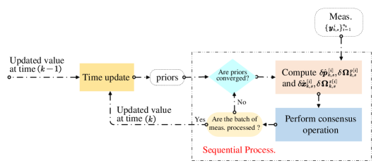
Figure 4: Block diagram of the proposed DWLSF.

The DWLSF involves the temporal evolution, sequential processing, and consensus iteration blocks (for detail, see Fig. 4). The detailed DWLSF is collected in Algorithm 2.

1 Initialization: $\hat{\bm{x}}_{1,s}^{[0]}$, $\hat{\bm{p}}_{1,s}^{[0]}$, $\mathbf{\Omega}_{1,s}^{x[0]}$, and $\mathbf{\Omega}_{1,s}^{p[0]}$ ;

2 for $k\leftarrow 1,2,\cdots$ // scan time  do

3       Data: $\{\bm{y}_{k,s}^{i}\}^{n_{k}}_{i=1}(s\in\mathcal{N})$ ;

4       Initialization: $\hat{\bm{x}}_{k,s}^{[0]}$, $\hat{\bm{p}}_{k,s}^{[0]}$, $\mathbf{\Omega}_{k,s}^{x[0]}$, and $\mathbf{\Omega}_{k,s}^{p[0]}$ ;

5      

6      for $i=1,2,\cdots,n_{k}$ // sequential  do

7            Compute consensus quantities ;

8             if Converged priors then

9                  using (43) and (45a), compute $\delta\hat{\bm{x}}^{[i]}_{k,s},\delta\mathbf{\Omega}^{x[i]}_{k,s},\delta\hat{\bm{p}}^{[i]}_{k,s},\delta\mathbf{\Omega}^{p[i]}_{k,s}$ via (38) and (39)

10            else

11                  using (44) and (45b), compute $\delta\hat{\bm{x}}^{[i]}_{k,s},\delta\mathbf{\Omega}^{x[i]}_{k,s},\delta\hat{\bm{p}}^{[i]}_{k,s},\delta\mathbf{\Omega}^{p[i]}_{k,s}$ via (38) and (39)

12             end if

13            Consensus operation ;

14             set $\delta\hat{\bm{x}}^{[i]}_{k,s}(0)\leftarrow\delta\hat{\bm{x}}^{[i]}_{k,s}$ , $\delta\mathbf{\Omega}^{x[i]}_{k,s}(0)\leftarrow\delta\mathbf{\Omega}^{x[i]}_{k,s}$, $\delta\hat{\bm{p}}^{[i]}_{k,s}(0)\leftarrow\delta\hat{\bm{p}}^{[i]}_{k,s}$, $\delta\mathbf{\Omega}^{p[i]}_{k,s}(0)\leftarrow\delta\mathbf{\Omega}^{p[i]}_{k,s}$ ;

15             for $l=0,\cdots,L-1$ do

16                  perform AC on $\delta\hat{\bm{x}}^{[i]}_{k,s},\delta\mathbf{\Omega}^{x[i]}_{k,s},\delta\hat{\bm{p}}^{[i]}_{k,s},\delta\mathbf{\Omega}^{p[i]}_{k,s}$

17             end for

18            compute $\hat{\bm{x}}_{k,s}^{[i]},\mathbf{\Omega}_{k,s}^{x[i]},\hat{\bm{p}}_{k,s}^{[i]},\mathbf{\Omega}_{k,s}^{p[i]}$ via (40) and (41)

19       end for

20      Output1: $\hat{\bm{x}}_{k,s}\leftarrow\hat{\bm{x}}_{k,s}^{[n_{k}]},\mathbf{C}_{k,s}^{x}\leftarrow\left(\mathbf{\Omega}_{k,s}^{x[n_{k}]}\right)^{-1}$ ;

21       Output2: $\hat{\bm{p}}_{k,s}\leftarrow\hat{\bm{p}}_{k,s}^{[n_{k}]},\mathbf{C}_{k,s}^{p}\leftarrow\left(\mathbf{\Omega}_{k,s}^{p[n_{k}]}\right)^{-1}$ ;

22       compute $\hat{\bm{x}}_{k+1,s}^{[0]},\mathbf{\Omega}_{k+1,s}^{x[0]},\hat{\bm{p}}_{k+1,s}^{[0]},\mathbf{\Omega}_{k+1,s}^{p[0]}$ via (24) and (25)

23 end for

Algorithm 2 DWLSF Filter

Remark 3

• The number of iterations $L$ linearly increases both computation and communication burdens. Hence, its value is usually set to be a suitable value to balance the performance and cost, which renders the estimates on each node being asymptotically optimal.

• At the initial scan time $k=1$, the uncorrelated priors (i.e., (44) and (45b)) are used in the sequential processing process. Then for $k\geq 2$, (43) and (45a) should be used as the estimates across the nodes become correlated for the following time steps [37].

• If the priors converge, the information becomes redundant on each node, and thus dividing the information matrices by ${|\mathcal{N}|}$ is necessary to match the centralized estimates.

VI Numerical Examples

To evaluate the performance of CVM and MEM proposed in [14], we first integrate the two models into CWLSF to track a rectangular object over a network with single node. Then, under different prior conditions, we compare DWLSF with the two previous approaches in [38] and [29] (abbreviated as CI filter and DEOT filter, respectively) in terms of the estimate consensus, computation time and tracking error over a network including the “naive” nodes. All numerical simulations are operated in MATLAB–2019b running on a PC with processor Intel(R) Core(TM) i7-10510U CPU @ 1.8GHz 2.3GHz and with 20GB RAM.

VI-A Performance evaluation on CVM and MEM model

To examine the effectiveness of CVM and MEM on different tracking applications, we conduct two experiments: 1) the orientation is aligned to the direction of velocity; 2) the orientation does not move exactly along the direction of velocity. We assess the position and extent errors simultaneously by the Optimal Sub-Pattern Assignment (OSPA) distance [13].

VI-A1 Object moves along the orientation

In this scenario (S1), the EO is a rectangular object with lengths $3$ and $4$ meters. The object moves with a nearly constant velocity $v=1.5\mathrm{m/s}$ following the trajectory shown in Fig. 5. The initial position of the object is at the origin of coordinates, and its orientation is consistent with the direction of velocity. Table II collects the parameters used in CWLSFs.

TABLE II: Parameter Setting in S1

Categories	Para.	Specification
Common para.	Scan time	$\mathrm{T}=3$ s
	Mea. Cov.	$\mathbf{C}^{v}=\mathrm{diag}(\frac{1}{3},\frac{1}{3})$
	Multip. noise Cov.	$\mathbf{C}^{h}=\frac{1}{3}\mathbf{I}_{2}$
	Kine. transition matrix	$\mathbf{F}_{k}^{s}=\begin{bmatrix}1&0&\mathrm{T}&0\\ 0&1&0&\mathrm{T}\\ 0&0&1&0\\ 0&0&0&1\end{bmatrix}$
	Process Cov. in Kine.	$\mathbf{C}^{x}_{w}=\mathrm{diag}(50,50,1,1)$
	Cov. in Extent	$\mathbf{C}_{1}^{p[0]}=\mathrm{diag}(0.36,\frac{1}{500},\frac{1}{50})$
	Cov. in Kine.	$\mathbf{C}_{1}^{x[0]}=\mathrm{diag}(2,2,\frac{1}{5},\frac{1}{5})$
	Extent transition matrix	$\mathbf{F}_{k}^{p}=\mathbf{I}_{3}$
	No. of Meas.	$\lambda=7$
MEM	Process Cov. in Extent	$\mathbf{C}^{p}_{w}=\mathrm{diag}(0.05,\frac{1}{500},\frac{1}{50})$
CVM	Process Cov. in Extent	$\mathbf{C}^{p}_{w}=\mathrm{diag}(0.3,\frac{1}{500},\frac{1}{220})$

Fig. 5 gives the true trajectory and overall tracking results over $M=50$ Monte Carlo runs. As shown in Fig. 5, CWLSF-CVM has better precision in comparison with CWLSF-MEM, especially during the turning phase and final moving phase. This because CVM indeed describes the tight relation between the velocity and orientation, so that when the object’s motion pattern changes, such as turning maneuvering, CWLSF-CVM quickly captures the change to modify its filtering gain. Fig. 6 gives the OSPA distance, and the result provides a direct conclusion on the advantage of CWLSF-CVM.

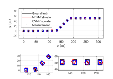
Figure 5: True trajectory and overall tracking results (per 3 scan times)

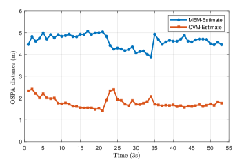
Figure 6: OSPA distance

VI-A2 Object moves with a drift

In this scenario (S2), the EO is a rectangular object with lengths $3$ and $4$ meters. The object moves with a nearly constant velocity $v=1.5\mathrm{m/s}$ following the trajectory shown in Fig. 7. The initial position of the object is at the origin of coordinates, and its orientation is a constant value $\frac{\pi}{4}$. Table III collects the parameters used in S2, and the other parameters are given in Table II.

TABLE III: Parameter Setting in S2

Categories	Para.	Specification
Common para.	Cov. in Extent	$\mathbf{C}_{1}^{p[0]}=\mathrm{diag}(0.0.1,\frac{1}{500},\frac{1}{100})$
MEM	Process Cov. in Extent	$\mathbf{C}^{p}_{w}=\mathrm{diag}(0.015,\frac{1}{400},\frac{1}{300})$
CVM	Process Cov. in Extent	$\mathbf{C}^{p}_{w}=\mathrm{diag}(0.5,\frac{1}{400},\frac{1}{300})$

Fig. 7 gives the true trajectory and overall tracking results over $M=50$ Monte Carlo runs. As expected, CWLSF-CVM outperforms CWLSF-MEM as a whole. The reason is that CVM allows objects to do a drift motion, i.e., a mismatch between the orientation and direction of their velocity, while MEM assumes that objects move along their orientation. Fig. 8 shows that CWLSF-CVM has lower OSPA distance than that of CWLSF-MEM, which validates the superiority on CVM.

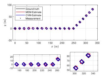
Figure 7: True trajectory and overall tracking results (per 3 scan times)

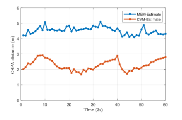
Figure 8: OSPA distance

VI-B Performance evaluation in a distributed scenario

In this scenario (S3), the network deploys $9$ nodes to monitor a $[0,500]\mathrm{m}\times[0,500]\mathrm{m}$ space. The sensing range is $200$m, and sensing azimuth spans from $0^{\circ}$ to $360^{\circ}$ for all sensors. Fig. 9 gives an example for such a network. Here, the considered EO is an elliptical object with lengths of the semi-axes $35$m and $30$m. The initial position of the object is at $[25,300]$, and then moves with a nearly constant velocity $v=\frac{100}{36}\mathrm{m/s}$ following a similar trajectory as in [39]. A sensor has measurements of the object only if the ground truth position of the object is within the sensor’s FoV.

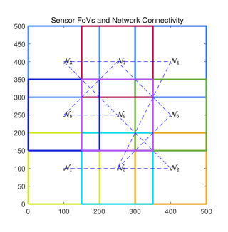
Figure 9: FoVs and network connectivity. The sensor FoVs are shown in squares. There are $9$ sensors in this example. The blue dotted lines represent the network connectivity.

Since DWLSF is guaranteed to converge to the centralized estimates only if the initial priors are equal, we testify the robustness of DWLSF in three cases: the equal priors, uncorrelated and unequal priors, and correlated and unequal priors. The comparison results are the Gaussian Wasserstein distance (GWD) [13, 14] for assessing both the position and extent errors, and a metric, Averaged consensus estimate error (ACEE), for testifying the estimate difference between different nodes. Moreover, considering that the number of iterations has a critical impact on filters’ performance, we check how many iterations $L$ could achieve a stable behavior.

VI-B1 Equal priors

If the priors are equal for all nodes, which means the priors have converged at the initial scan time $k=1$. Thus, the prior covariances w.r.t kinematics are set to $\mathbf{C}_{1,s}^{x[0]}=\mathrm{diag}(50,50,10,10)$, and the prior covariances w.r.t extent are set to $\mathbf{C}_{1,s}^{p[0]}=\mathrm{diag}(0.01,0.1,0.1)$ for all nodes. The other parameters are given in Table IV.

TABLE IV: Parameter Setting in S3

Categories	Para.	Specification
Common para.	Scan time	$\mathrm{T}=5$ s
	Mea. Cov.	$\mathbf{C}^{v}=\mathrm{diag}(40,20)$
	Multip. noise Cov.	$\mathbf{C}^{h}=\frac{1}{4}\mathbf{I}_{2}$
	Kine. transition matrix	as shown in Table II
	Process Cov. in Kine.	$\mathbf{C}^{x}_{w}=\mathrm{diag}(10^{2},10^{2},1,1)$
	Prior cov. in CWLSF	$\mathbf{C}_{1}^{x[0]}=\mathrm{diag}(2,2,\frac{1}{2},\frac{1}{2})$
	Prior cov. in CWLSF	$\mathbf{C}_{1}^{p[0]}=\mathrm{diag}(2\times 10^{-3},10^{-3},10^{-4})$
	Consensus para.	$\xi=0.65/\triangle\max$
	Maximum degree	$\triangle\max=2$
	Extent transition matrix	$\mathbf{F}_{k}^{p}=\mathbf{I}_{3}$
	No. of Meas.	$\lambda=10$
Others filter	Process Cov. in Extent	$\mathbf{C}^{p}_{w}=\mathrm{diag}(0.05,10^{-3},10^{-4})$
CVM	Process Cov. in Extent	$\mathbf{C}^{p}_{w}=\mathrm{diag}(2\times 10^{-3},10^{-3},10^{-4})$

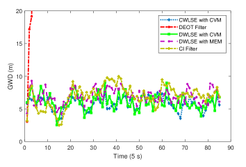
Figure 10: GWD distance with $L=10$

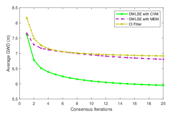
Figure 11: Average GWD distance with different iterations

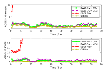
Figure 12: ACEEs in kinematics and extent ($L=10$)

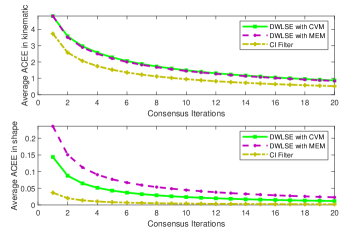
Figure 13: Average ACEEs with different iterations

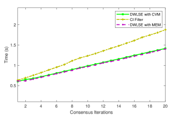
Figure 14: Computational time with different iterations.

Fig. 11 shows the GWD distance of four examined filters. The DWLSF-CVM performs better than the other distributed filters, as CVM delivers the merit that describes the correlation between the velocity and orientation to DWLSF-CVM. DEOT filter is divergent in S3, because it assumes that each node in network detects the object during the whole tracking process. However, the assumption is no longer valid in a realistic network as in S3. The reason why CI filter has a lager GWD distance than DWLSFs is that the cross-covariances across different nodes are not incorporated in its estimation framework.

As expected, the average GWD distance decreases with the increased number of iterations, and this phenomenon is more apparent in DWLSF-CVM (see Fig. 11). Combined the results in Figs. 11-11, we can anticipate that DWLSF-CVM will approach to CWLSF-CVM almost tightly when $L>10$, which verifies the validity of the proposed consensus scheme.

Fig. 13 shows the difference between nodes in the kinematics and extent estimate. Both DWLSFs give a satisfied consensus result in the kinematics, but DWLSF-CVM has a smaller difference in the extent. Although CI filter has a lower ACEE, one cannot declare that it outperforms DWLSEs. Because when the GWD distance is large, even if the ACEE is small, it does not make any sense. Again, DEOT filter fails to yield a satisfied consensus result.

Fig. 13 shows the average ACEE under different iterations. Compared with DWLSF-MEM, DWLSF-CVM and CI filter require fewer iterations to generate a stable consensus result.

Fig. 14 compares the average computational costs per tracking process on different filters under different iterations. For a given $l$, DWLSFs almost consume $70\%$ computational resource of CI filter. This merit makes DWLSFs more appealing on a computer with limited computing capability.

VI-B2 Uncorrelated and unequal priors

In this case, the prior covariances w.r.t kinematics are set to $\mathbf{C}_{1,s}^{x[0]}=\mathrm{diag}(100,100,10,10).*\mathrm{diag}(\mathrm{rand}(1,4))$, and the prior covariances w.r.t extent are set to $\mathbf{C}_{1,s}^{p[0]}=\mathrm{diag}(1,7,7).*\mathrm{diag}(\mathrm{rand}(1,3))$ for all nodes. The other parameters are given in Table IV.

As shown in Figs. 16-16, even in the case that the priors are unequal and uncorrelated, DWLSF-CVM still follows CWLSF-CVM closely with increased iterations. This because DWLSF is a consensus-based filter and irrespective of the initial condition, after several time steps or iterations, the priors have met the converged condition. Also, DWLSF-CVM has minimum GWD distance in comparison with the other distributed filters under the case.

For the estimate difference between nodes, both DWLSFs give a satisfying consensus result as shown in Figs. 18-18. These results prove the robustness of DWLSF in terms of the consensus. The ACEEs on CI filter are similar to DWLSFs’ result, while the ACEEs on DEOT are beyond a reasonable range.

The average computational costs per tracking process under different iterations are given in Fig. 19. Combined with the results in Figs. 16-16, we see that DWLSFs require less computational resources to yield a pretty performance in comparison with CI filter.

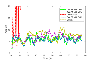
Figure 15: GWD distance with $L=10$

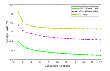
Figure 16: Average GWD distance with different iterations

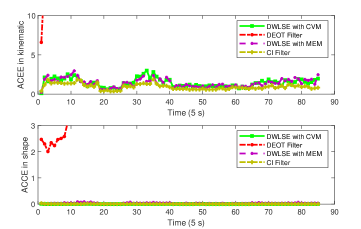
Figure 17: ACEEs in kinematics and extent ($L=10$)

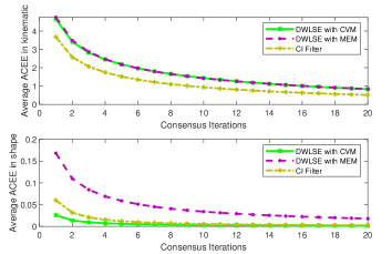
Figure 18: Average ACEEs with different iterations

Figure 19: Computational time with different iterations.

VI-B3 Correlated and unequal priors

In this case, the prior covariances w.r.t kinematics are set to $\mathbf{C}_{1,s}^{x[0]}=\mathrm{diag}(100,100,10,10).*\mathrm{diag}(\mathrm{rand}(1,4))$, and the prior covariances w.r.t extent are set to $\mathbf{C}_{1,s}^{p[0]}=\mathrm{diag}(1,7,7).*\mathrm{diag}(\mathrm{rand}(1,3))$, with $\rho=0.5$ correlation coefficient between the priors across nodes. The other parameters are given in Table IV.

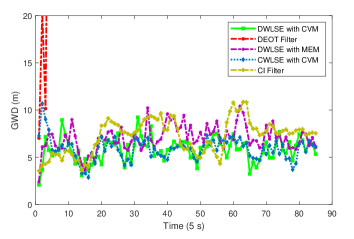
Figure 20: GWD distance with $L=10$

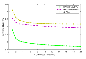
Figure 21: Average GWD distance with different iteration

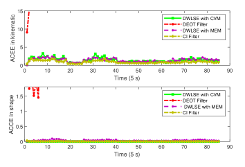
Figure 22: ACEEs in kinematics and extent ($L=10$)

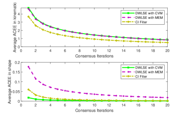
Figure 23: Average ACEEs with different iterations

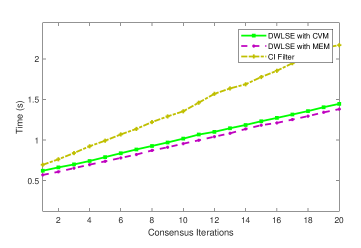
Figure 24: Computational time with different iterations.

From the results in Figs. 21-21, DWLSE-CVM also approaches to the result of CWLSE-CVM when the priors are unequal and correlated. As for the ACEE, average ACEE and computation time (see Figs. 22-24), the same conclusion is drawn as given in section VI-B2.

VII Conclusion

This study first proposes a coupled velocity state-space model. This model is capable of describing the correlation between the object’s orientation and velocity, which allows the model to further detect changes in the EO’s motion mode and improve the performance of the corresponding filter. Then, without losing any first and second moment information, the proposed model is separated into two pseudo-linearized models with only additive noise. Finally, under a network with “naive” nodes, we use the two models to design a distributed WLS filter that takes the cross-covariances between nodes into account. The distributed filter converges to the corresponding centralized form in three different situations, which indicates its robustness when the convergence condition is not met. Potential future works could ponder how to achieve the distributed filter in a heterogeneous sensor network [40, 41] or under multiple constraints [42, 43, 44].

Appendix A Proof of proposition 1

Proof:

For brevity, we first derive the partial derivatives of $\frac{v_{k}^{\mathsf{x}}}{\|\bm{\vartheta}_{k}\|}$ and $\frac{v_{k}^{\mathsf{y}}}{\|\bm{\vartheta}_{k}\|}$ with respect to $v_{k}^{\mathsf{x}}$ and $v_{k}^{\mathsf{y}}$, respectively, at the $[i-1]$-th velocity estimate ${{\bm{\vartheta}}_{k}^{[i-1]}}$ as

$$\left\{\begin{lgathered}d1=\left.\frac{\partial v_{k}^{\mathsf{x}}/\|\bm{\vartheta}_{k}\|}{\partial v_{k}^{\mathsf{x}}}\right|_{\hat{\bm{\vartheta}}_{k}^{[i-1]}}=\left.\frac{1}{\|\bm{\vartheta}_{k}\|}-\frac{(v_{k}^{\mathsf{x}})^{2}}{(\|\bm{\vartheta}_{k}\|)^{3}}\right|_{\hat{\bm{\vartheta}}_{k}^{[i-1]}},\\ d2=\left.\frac{\partial v_{k}^{\mathsf{y}}/\|\bm{\vartheta}_{k}\|}{\partial v_{k}^{\mathsf{y}}}\right|_{\hat{\bm{\vartheta}}_{k}^{[i-1]}}=\left.\frac{1}{\|\bm{\vartheta}_{k}\|}-\frac{(v_{k}^{\mathsf{y}})^{2}}{(\|\bm{\vartheta}_{k}\|)^{3}}\right|_{\hat{\bm{\vartheta}}_{k}^{[i-1]}},\\ d3=\left.\frac{\partial v_{k}^{\mathsf{y}}/\|\bm{\vartheta}_{k}\|}{\partial v_{k}^{\mathsf{x}}}=\frac{\partial v_{k}^{\mathsf{x}}/\|\bm{\vartheta}_{k}\|}{\partial v_{k}^{\mathsf{y}}}\right|_{\hat{\bm{\vartheta}}_{k}^{[i-1]}}=\left.-\frac{v_{k}^{\mathsf{x}}v_{k}^{\mathsf{y}}}{(\|\bm{\vartheta}_{k}\|)^{3}}\right|_{\hat{\bm{\vartheta}}_{k}^{[i-1]}}.\end{lgathered}d1=\left.\frac{\partial v_{k}^{\mathsf{x}}/\|\bm{\vartheta}_{k}\|}{\partial v_{k}^{\mathsf{x}}}\right|_{\hat{\bm{\vartheta}}_{k}^{[i-1]}}=\left.\frac{1}{\|\bm{\vartheta}_{k}\|}-\frac{(v_{k}^{\mathsf{x}})^{2}}{(\|\bm{\vartheta}_{k}\|)^{3}}\right|_{\hat{\bm{\vartheta}}_{k}^{[i-1]}},\\ d2=\left.\frac{\partial v_{k}^{\mathsf{y}}/\|\bm{\vartheta}_{k}\|}{\partial v_{k}^{\mathsf{y}}}\right|_{\hat{\bm{\vartheta}}_{k}^{[i-1]}}=\left.\frac{1}{\|\bm{\vartheta}_{k}\|}-\frac{(v_{k}^{\mathsf{y}})^{2}}{(\|\bm{\vartheta}_{k}\|)^{3}}\right|_{\hat{\bm{\vartheta}}_{k}^{[i-1]}},\\ d3=\left.\frac{\partial v_{k}^{\mathsf{y}}/\|\bm{\vartheta}_{k}\|}{\partial v_{k}^{\mathsf{x}}}=\frac{\partial v_{k}^{\mathsf{x}}/\|\bm{\vartheta}_{k}\|}{\partial v_{k}^{\mathsf{y}}}\right|_{\hat{\bm{\vartheta}}_{k}^{[i-1]}}=\left.-\frac{v_{k}^{\mathsf{x}}v_{k}^{\mathsf{y}}}{(\|\bm{\vartheta}_{k}\|)^{3}}\right|_{\hat{\bm{\vartheta}}_{k}^{[i-1]}}.\right.$$ (46)

Considering that the true extent $\bm{p}_{k}$ and velocity $\bm{\vartheta}_{k}$ are unknown in the coefficient matrix $\mathbf{S}_{k}$, performing the first-order Taylor series expansion of term $\mathbf{S}_{k}\bm{h}_{k,s}^{i}$ in (3) around the ${[i-1]}$-th extent $\hat{\bm{p}}_{k}^{[i-1]}$ and velocity $\hat{\bm{\vartheta}}_{k}^{[i-1]}$, respectively, and keeping $\bm{h}_{k,s}^{[i]}$ as a random variable yields

$$\begin{split}\mathbf{S}_{k}\bm{h}_{k,s}^{i}\approx&\underbrace{\hat{\mathbf{S}}_{k}^{[i-1]}\bm{h}_{k,s}^{i}}_{\mathrm{I}}+\underbrace{\left[\begin{array}[]{c}\left(\bm{h}_{k,s}^{i}\right)^{\mathsf{T}}\hat{\mathbf{J}}_{1k,p}^{[i-1]}\\ \left(\bm{h}_{k,s}^{i}\right)^{\mathsf{T}}\hat{\mathbf{J}}_{2k,p}^{[i-1]}\end{array}\right]\left(\bm{p}_{k}-\hat{\bm{p}}_{k}^{[i-1]}\right)}_{\mathrm{II}}\\ &+\underbrace{\left[\begin{array}[]{c}\left(\bm{h}_{k,s}^{i}\right)^{\mathsf{T}}\hat{\mathbf{J}}_{1k,v}^{[i-1]}\\ \left(\bm{h}_{k,s}^{i}\right)^{\mathsf{T}}\hat{\mathbf{J}}_{2k,v}^{[i-1]}\end{array}\right]\left(\bm{\vartheta}_{k}-\hat{\bm{\vartheta}}_{k}^{[i-1]}\right)}_{\mathrm{III}}\end{split}$$ (47)

where $\mathbf{J}_{1k,v}$ and $\mathbf{J}_{2k,v}$ are the Jacobian matrices of the first row $\mathbf{S}_{1,k}$ and second row $\mathbf{S}_{2,k}$ of $\mathbf{S}_{k}$ at the ${[i-1]}$-th velocity estimate $\hat{\bm{\vartheta}}_{k}^{[i-1]}$ (see (48) and (49)), and $\mathbf{J}_{1k,p}$ and $\mathbf{J}_{2k,p}$ are the Jacobian matrices of the first row $\mathbf{S}_{1,k}$ and second row $\mathbf{S}_{2,k}$ of $\mathbf{S}_{k}$ at the ${[i-1]}$-th extent estimate $\hat{\bm{p}}_{k}^{[i-1]}$ (see (50) and (51)).

$$\mathbf{J}_{1k,v}=\left.\frac{\partial\mathbf{S}_{1,k}}{\partial\bm{\vartheta}_{k}}\right|_{\hat{\bm{\vartheta}}_{k}^{[i-1]}}=\left.\begin{bmatrix}l_{k,1}(d3\sin{\beta_{k}}+d1\cos{\beta_{k}})&l_{k,1}(d2\sin{\beta_{k}}+d3\cos{\beta_{k}})\\ l_{k,2}(d1\sin{\beta_{k}}-d3\cos{\beta_{k}})&l_{k,2}(d3\sin{\beta_{k}}-d2\cos{\beta_{k}})\end{bmatrix}\right|_{\hat{\bm{\vartheta}}_{k}^{[i-1]}},$$ (48)

$$\mathbf{J}_{2k,v}=\left.\frac{{\color[rgb]{1,0,0}\partial\mathbf{S}_{2,k}}}{\partial\bm{\vartheta}_{k}}\right|_{\hat{\bm{\vartheta}}_{k}^{[i-1]}}=\left.\begin{bmatrix}l_{k,1}(d3\cos{\beta_{k}}-d1\sin{\beta_{k}})&l_{k,1}(d2\cos{\beta_{k}}-d3\sin{\beta_{k}})\\ {\color[rgb]{1,0,0}l_{k,2}(d3\sin{\beta_{k}}+d1\cos{\beta_{k}})}&l_{k,2}(d2\sin{\beta_{k}}+d3\cos{\beta_{k}})\end{bmatrix}\right|_{\hat{\bm{\vartheta}}_{k}^{[i-1]}},$$ (49)

$$\mathbf{J}_{1k,p}=\left.\frac{{\color[rgb]{1,0,0}\partial\mathbf{S}_{1,k}}}{\partial\bm{p}_{k}}\right|_{\hat{\bm{p}}_{k}^{[i-1]}}=\left.\begin{bmatrix}\frac{v_{k}^{\mathsf{x}}\cos{\beta_{k}}+v_{k}^{\mathsf{y}}\sin{\beta_{k}}}{\|\bm{\vartheta}_{k}\|}&0&\frac{l_{k,1}(v_{k}^{\mathsf{y}}\cos{\beta_{k}}-v_{k}^{\mathsf{x}}\sin{\beta_{k}})}{\|\bm{\vartheta}_{k}\|}\\ 0&\frac{v_{k}^{\mathsf{x}}\sin{\beta_{k}}-v_{k}^{\mathsf{y}}\cos{\beta_{k}}}{\|\bm{\vartheta}_{k}\|}&\frac{{\color[rgb]{1,0,0}l_{k,2}}(v_{k}^{\mathsf{x}}\cos{\beta_{k}}+v_{k}^{\mathsf{y}}\sin{\beta_{k}})}{\|\bm{\vartheta}_{k}\|}\end{bmatrix}\right|_{\hat{\bm{p}}_{k}^{[i-1]}},$$ (50)

$${\color[rgb]{1,0,0}\mathbf{J}_{2k,p}}=\left.\frac{\partial\mathbf{S}_{2,k}}{\partial\bm{p}_{k}}\right|_{\hat{\bm{p}}_{k}^{[i-1]}}=\left.\begin{bmatrix}\frac{v_{k}^{\mathsf{y}}\cos{\beta_{k}}-v_{k}^{\mathsf{x}}\sin{\beta_{k}}}{\|\bm{\vartheta}_{k}\|}&0&-\frac{l_{k,1}(v_{k}^{\mathsf{y}}\sin{\beta_{k}}+v_{k}^{\mathsf{x}}\cos{\beta_{k}})}{\|\bm{\vartheta}_{k}\|}\\ 0&\frac{v_{k}^{\mathsf{y}}\sin{\beta_{k}}+v_{k}^{\mathsf{x}}\cos{\beta_{k}}}{\|\bm{\vartheta}_{k}\|}&\frac{{\color[rgb]{1,0,0}l_{k,2}}(v_{k}^{\mathsf{y}}\cos{\beta_{k}}-v_{k}^{\mathsf{x}}\sin{\beta_{k}})}{\|\bm{\vartheta}_{k}\|}\end{bmatrix}\right|_{\hat{\bm{p}}_{k}^{[i-1]}}.$$ (51)

Substituting (47) into (3), using the fact that the terms ${\mathrm{II}}$ and ${\mathrm{III}}$ in (47) are scalar, the residual covariance about $\bm{y}_{k,s}^{i}$ in (3) is calculated as

$$\mathbf{C}_{k,s}^{y[i]}=\mathbf{H}\mathbf{C}_{k}^{x[i-1]}\mathbf{H}^{\mathsf{T}}+\mathbf{C}^{\mathrm{\@slowromancap i@}}+\mathbf{C}^{\mathrm{\@slowromancap ii@}}+\mathbf{C}^{\mathrm{\@slowromancap iii@}}+\mathbf{C}_{s}^{v},$$ (52)

and then (3) is rewritten as (6). The proof is complete. ∎

Appendix B Proof of proposition 2

Proof:

It is shown that (10) does not exist a directly linear/nonlinear mapping between $\bm{p}_{k}$ and $\mathbf{Y}_{k,s}^{[i]}$. To extract the term $\bm{p}_{k}$ from (10), substituting (47) into (3) yields

$$\bm{y}_{k,s}^{i}\approx\;\mathbf{H}\bm{x}_{k}+\hat{\mathbf{S}}_{k}^{[i-1]}\bm{h}_{k,s}^{i}+\left[\begin{array}[]{c}\left(\bm{h}_{k,s}^{i}\right)^{\mathsf{T}}\hat{\mathbf{J}}_{1k,p}^{[i-1]}\\ \left(\bm{h}_{k,s}^{i}\right)^{\mathsf{T}}\hat{\mathbf{J}}_{2k,p}^{[i-1]}\end{array}\right]\left(\bm{p}_{k}-\hat{\bm{p}}_{k}^{[i-1]}\right)+\left[\begin{array}[]{c}\left(\bm{h}_{k,s}^{i}\right)^{\mathsf{T}}\hat{\mathbf{J}}_{1k,v}^{[i-1]}\\ \left(\bm{h}_{k,s}^{i}\right)^{\mathsf{T}}\hat{\mathbf{J}}_{2k,v}^{[i-1]}\end{array}\right]\left(\bm{\vartheta}_{k}-\hat{\bm{\vartheta}}_{k}^{[i-1]}\right)+\bm{v}_{k,s}^{i}:=\tilde{\bm{y}}_{k,s}^{i}.$$ (53)

Further, substituting (53) into (10) gives

$$\mathbf{Y}_{k,s}^{[i]}\approx {}\mathbf{F}\left(\left(\tilde{\bm{y}}_{k,s}^{i}-\mathbf{H}\hat{\bm{x}}_{k}^{[i-1]}\right)\otimes\Big{(}\cdot\Big{)}\right)$$ (54a)

$$:= {}[Y_{1}^{2}\>Y_{2}^{2}\>Y_{1}Y_{2}]^{\mathsf{T}}$$ (54b)

where the notation $\left(\cdot\right)$ denotes the term right before it.

Next, our goal is using (54) to construct an equivalent measurement model $\mathbf{Y}_{k,s}^{[i]}\approx\mathbf{H}^{p}_{k}\bm{p}_{k}+\bm{v}_{k,s}^{p[i]}$ about $\bm{p}_{k}$, where $\mathbf{H}^{p}_{k}$ is the measurement matrix, and $\bm{v}_{k,s}^{p[i]}$ is measurement noise. Meanwhile, the first and second moments of the model should equal to the expectation and covariance of (10) as much as possible. For the clarity, denote $\mathbf{H}\bm{x}_{k}-\mathbf{H}\hat{\bm{x}}_{k}^{[i-1]}:=[\tilde{x}_{1}\;\tilde{x}_{2}]^{\mathsf{T}}$, $\mathbf{H}\mathbf{C}_{k}^{x[i-1]}\mathbf{H}^{\mathsf{T}}:=\left[\begin{smallmatrix}c^{x}_{11}&c^{x}_{12}\\ c^{x}_{21}&c^{x}_{22}\end{smallmatrix}\right]$, $\mathbf{C}_{k,s}^{y[i]}:=\left[\begin{smallmatrix}c^{y}_{11}&c^{y}_{12}\\ c^{y}_{21}&c^{y}_{22}\end{smallmatrix}\right]$, $\hat{\mathbf{S}}_{k}^{[i-1]}:=[\hat{\mathbf{S}}_{1}^{\mathsf{T}}\;\hat{\mathbf{S}}_{2}^{\mathsf{T}}]^{\mathsf{T}}$, $\bm{v}_{k,s}^{[i]}:=[v_{1}\;v_{2}]^{\mathsf{T}}$, $\mathrm{Cov}(\bm{v}_{k,s}^{[i]}):=\mathrm{diag}\left[\begin{smallmatrix}\sigma_{1}^{2}&0\\ 0&\sigma_{2}^{2}\end{smallmatrix}\right]$, and omit the superscript $[\cdot]$, time index $k$, and sensor node index $s$. Then, (54b) is further expanded as follows

$$Y_{1}^{2}=\left(\tilde{x}_{1}+\hat{\mathbf{S}}_{1}\bm{h}+\bm{h}^{\mathsf{T}}\hat{\mathbf{J}}_{1,p}(\bm{p}-\hat{\bm{p}})+\bm{h}^{\mathsf{T}}\hat{\mathbf{J}}_{1,v}(\bm{\vartheta}-\hat{\bm{\vartheta}})+v_{1}\right)^{2}-2\hat{\mathbf{S}}_{1}\mathbf{C}^{h}\hat{\mathbf{J}}_{1,p}\bm{p}+2\hat{\mathbf{S}}_{1}\mathbf{C}^{h}\hat{\mathbf{J}}_{1,p}\bm{p},$$ (55a)

$$Y_{1}^{2}=\left(\tilde{x}_{2}+\hat{\mathbf{S}}_{2}\bm{h}+\bm{h}^{\mathsf{T}}\hat{\mathbf{J}}_{2,p}(\bm{p}-\hat{\bm{p}})+\bm{h}^{\mathsf{T}}\hat{\mathbf{J}}_{2,v}(\bm{\vartheta}-\hat{\bm{\vartheta}})+v_{2}\right)^{2}-2\hat{\mathbf{S}}_{2}\mathbf{C}^{h}\hat{\mathbf{J}}_{2,p}\bm{p}+2\hat{\mathbf{S}}_{2}\mathbf{C}^{h}\hat{\mathbf{J}}_{2,p}\bm{p},$$ (55b)

$$\begin{split}Y_{1}Y_{2}=&\left(\tilde{x}_{2}+\hat{\mathbf{S}}_{2}\bm{h}+\bm{h}^{\mathsf{T}}\hat{\mathbf{J}}_{2,p}(\bm{p}-\hat{\bm{p}})+\bm{h}^{\mathsf{T}}\hat{\mathbf{J}}_{2,v}(\bm{\vartheta}-\hat{\bm{\vartheta}})+v_{2}\right)\left(\tilde{x}_{1}+\hat{\mathbf{S}}_{1}\bm{h}+\bm{h}^{\mathsf{T}}\hat{\mathbf{J}}_{1,p}(\bm{p}-\hat{\bm{p}})+\bm{h}^{\mathsf{T}}\hat{\mathbf{J}}_{1,v}(\bm{\vartheta}-\hat{\bm{\vartheta}})+v_{1}\right)\\ &+\hat{\mathbf{S}}_{2}\mathbf{C}^{h}\hat{\mathbf{J}}_{1,p}\bm{p}+\hat{\mathbf{S}}_{1}\mathbf{C}^{h}\hat{\mathbf{J}}_{2,p}\bm{p}-\hat{\mathbf{S}}_{2}\mathbf{C}^{h}\hat{\mathbf{J}}_{1,p}\bm{p}-\hat{\mathbf{S}}_{1}\mathbf{C}^{h}\hat{\mathbf{J}}_{2,p}\bm{p}.\end{split}$$ (55c)

The expectation of (55) is given as follows:

$$\mathbb{E}(Y_{1}^{2})=c_{11}^{x}+\hat{\mathbf{S}}_{1}\mathbf{C}^{h}\hat{\mathbf{S}}_{1}^{\mathsf{T}}+\mathrm{tr}(\mathbf{C}^{p}\hat{\mathbf{J}}_{1,v}^{\mathsf{T}}\mathbf{C}^{h}\hat{\mathbf{J}}_{1,v})+\mathrm{tr}(\mathbf{C}^{p}\hat{\mathbf{J}}_{1,p}^{\mathsf{T}}\mathbf{C}^{h}\hat{\mathbf{J}}_{1,p})+\sigma_{1}^{2}-2\hat{\mathbf{S}}_{1}\mathbf{C}^{h}\hat{\mathbf{J}}_{1,p}\bm{p}+2\hat{\mathbf{S}}_{1}\mathbf{C}^{h}\hat{\mathbf{J}}_{1,p}\bm{p},$$ (56a)

$$\mathbb{E}(Y_{2}^{2})=c_{22}^{x}+\hat{\mathbf{S}}_{2}\mathbf{C}^{h}\hat{\mathbf{S}}_{2}^{\mathsf{T}}+\mathrm{tr}(\mathbf{C}^{p}\hat{\mathbf{J}}_{2,v}^{\mathsf{T}}\mathbf{C}^{h}\hat{\mathbf{J}}_{2,v})+\mathrm{tr}(\mathbf{C}^{p}\hat{\mathbf{J}}_{2,p}^{\mathsf{T}}\mathbf{C}^{h}\hat{\mathbf{J}}_{2,p})+\sigma_{2}^{2}-2\hat{\mathbf{S}}_{2}\mathbf{C}^{h}\hat{\mathbf{J}}_{2,p}\bm{p}+2\hat{\mathbf{S}}_{2}\mathbf{C}^{h}\hat{\mathbf{J}}_{2,p}\bm{p},$$ (56b)

$$\mathbb{E}(Y_{1}Y_{2})=c_{12}^{x}+\hat{\mathbf{S}}_{1}\mathbf{C}^{h}\hat{\mathbf{S}}_{2}^{\mathsf{T}}+\mathrm{tr}(\mathbf{C}^{p}\hat{\mathbf{J}}_{1,v}^{\mathsf{T}}\mathbf{C}^{h}\hat{\mathbf{J}}_{2,v})+\mathrm{tr}(\mathbf{C}^{p}\hat{\mathbf{J}}_{1,p}^{\mathsf{T}}\mathbf{C}^{h}\hat{\mathbf{J}}_{2,p})+\hat{\mathbf{S}}_{2}\mathbf{C}^{h}\hat{\mathbf{J}}_{1,p}\bm{p}+\hat{\mathbf{S}}_{1}\mathbf{C}^{h}\hat{\mathbf{J}}_{2,p}\bm{p}-\hat{\mathbf{S}}_{2}\mathbf{C}^{h}\hat{\mathbf{J}}_{1,p}\bm{p}-\hat{\mathbf{S}}_{1}\mathbf{C}^{h}\hat{\mathbf{J}}_{2,p}\bm{p}.$$ (56c)

Equation (54a) implies $\mathbb{E}(Y_{1})=\mathbb{E}(Y_{2})=0$, $\mathrm{Cov}(Y_{1})=c_{11}^{y}$, $\mathrm{Cov}(Y_{1}Y_{2})=c_{12}^{y}$ and $\mathrm{Cov}(Y_{2})=c_{22}^{y}$. From Wick’s theorem [33], we have

$$\left\{\begin{lgathered}\mathbb{E}\{(Y_{1}^{2})^{2}\}=3(c_{11}^{y})^{2},\;\mathbb{E}\{(Y_{2}^{2})^{2}\}=3(c_{22}^{y})^{2},\;\mathbb{E}\{(Y_{1}^{3}Y_{2})\}=3(c_{11}^{y}c_{12}^{y})\\ \mathbb{E}\{(Y_{1}Y_{2}^{3})\}=3(c_{22}^{y}c_{12}^{y}),\;\mathbb{E}\{(Y_{1}^{2}Y_{2}^{2})\}=c_{11}^{y}c_{22}^{y}+2(c_{12}^{y})^{2}\end{lgathered}\mathbb{E}\{(Y_{1}^{2})^{2}\}=3(c_{11}^{y})^{2},\;\mathbb{E}\{(Y_{2}^{2})^{2}\}=3(c_{22}^{y})^{2},\;\mathbb{E}\{(Y_{1}^{3}Y_{2})\}=3(c_{11}^{y}c_{12}^{y})\\ \mathbb{E}\{(Y_{1}Y_{2}^{3})\}=3(c_{22}^{y}c_{12}^{y}),\;\mathbb{E}\{(Y_{1}^{2}Y_{2}^{2})\}=c_{11}^{y}c_{22}^{y}+2(c_{12}^{y})^{2}\right..$$ (57)

By rearranging (54b), (55), (56) and (57), we have

$$\left[\begin{array}[]{c}Y_{1}^{2}\\ Y_{2}^{2}\\ Y_{1}Y_{2}\end{array}\right]=\hat{\mathbf{M}}\bm{p}+\bm{v}^{p}$$ (58)

with expectation $\mathbf{F}\mathrm{vect}\left(\mathbf{C}^{y}\right)$ and covariance $\mathbf{F}\left(\mathbf{C}^{y}\otimes\mathbf{C}^{y}\right)(\mathbf{F}+\tilde{\mathbf{F}})^{\mathsf{T}}$. Then, we get the measurement model as shown in (14), and find the measurement matrix $\mathbf{H}^{p}=\hat{\mathbf{M}}$. The first and second moments of (58) are consistent with the results as shown in (11) and (12), respectively, which means that (58) matches the moments information in (10). Notice that using those terms in $\hat{\mathbf{M}}$ guarantees (54b) and (10) giving the same value on computing the cross-covariance between $\mathbf{Y}$ and $\bm{p}$, but choosing other terms do not satisfy this condition. Until now, the proof is complete. ∎

Zhifei Li received the M.E. and Ph.D. degrees in Information and Communication Engineering from the National University of Defense Technology, Hefei, China, in 2016 and 2020, respectively. During September 2019–July 2020, he was a Visiting Research Scalar in the the School of Automation at Northwestern Polytechnical University, Xi’an, China. He is currently a Lecturer with the School of Space Information, Space Engineering University, Beijing, China. His research interests include statistical signal processing, extended object tracking, multi-sensor control, distributed system design and data fusion.

Yan Liang received the B.E., M.E., and Ph.D. degrees from Northwestern Polytechnical University (NPU), Xi’an, China, in 1993, 1998, and 2001, respectively. He was a Postdoctoral Fellow with Tsinghua University, Beijing, China, from 2001 to 2003, a Research Fellow with the Hong Kong Polytechnic University, Hong Kong, from 2006 to 2006, and a Visiting Scholar with the University of Alberta, Edmonton, AB, Canada, from 2007 to 2008. Since 2009, he has been a Professor with the School of Automation, NPU. His research interests include estimation theory, information fusion, and target tracking.

Linfeng Xu (S’10-M’14) received the B.S. and M.S. degrees in mechatronic engineering from Northwestern Polytechnical University (NPU), Xi’an, China, in 2002 and 2005, respectively, and the Ph.D. degree in Control Science and Engineering from Xi’an Jiaotong University, China, in 2013. In October 2013, he joined the School of Automation at NPU and is currently working as an associate professor. During September 2017–September 2018, he was a visiting research fellow in the Department of Electrical Engineering at the University of New Orleans, LA, USA. He is also a member of the Laboratory of Information Fusion Technology, Ministry of Education, China. His research interests are in detection and estimation theory, target tracking, and air traffic control.

References

- [1] K. Granström, M. Baum, S. Reuter, “Extended object tracking: introduction, overview and applications,” J. Adv. Inf. Fusion, vol. 12, no. 2, pp. 139-174, 2017.
- [2] J. W. Koch, “Bayesian approach to extended object and cluster tracking using random matrices,” IEEE Trans. Aerosp. Electron. Syst., vol. 44, no. 3, pp. 1042-1059, 2008.
- [3] J. Lan and X. R. Li, “Tracking of extended object or target group using random matrix: new model and approach,” IEEE Trans. Aerosp. Electron. Syst., vol. 52, no. 6, pp. 2973-2989, 2016.
- [4] K. Granström and J. Bramstång, “Bayesian smoothing for the extended object random matrix model,”IEEE Trans. Signal Process., vol. 67, no. 14, pp. 3732-3742, 2019.
- [5] J. Lan and X. R. Li, “Extended object or group target tracking using random matrix with nonlinear measurements,” IEEE Trans. Signal Process., vol. 67, no. 19, pp. 5130-5142, 2019.
- [6] B. Tuncer and E. Özkan, “Random matrix based extended target tracking with orientation: a new model and inference,”IEEE Trans. Signal Process., vol. 69, pp. 1910-1923, 2021.
- [7] L. Zhang and J. Lan, “Extended object tracking using random matrix with skewness,”IEEE Trans. Signal Process., vol. 68, pp. 5107-5121, 2020.
- [8] L. Zhang and J. Lan, “Tracking of extended object using random matrix with non-uniformly distributed measurements,” ”IEEE Trans. Signal Process., vol. 69, pp. 3812-3825, 2021.
- [9] M. Baum and U. D. Hanebeck, “Shape tracking of extended objects and group targets with star-convex RHMs,” in Proc. 14th Int. Conf. Inf. Fusion, Chicago, IL, USA, July 2011, pp. 1-8.
- [10] M. Kumru and E. Özkan, “3D extended object tracking using recursive Gaussian processes,” in Proc. 2018 21st Int. Conf. Inf. Fusion, Cambridge, UK, July 2018, pp. 1-8.
- [11] W. Aftab, R. Hostettler, A. De Freitas, M. Arvaneh and L. Mihaylova, “Spatio-temporal Gaussian process models for extended and group object tracking with irregular shapes,” IEEE Trans. Veh. Technol., vol. 68, no. 3, pp. 2137-2151, 2019.
- [12] S. Lee and J. McBride, “Extended object tracking via positive and negative information fusion,” IEEE Trans. Signal Process., vol. 67, no. 7, pp. 1812-1823, 2019.
- [13] S. Yang and M. Baum, “Second-order extended Kalman filter for extended object and group tracking,” in Proc. 2016 19st Int. Conf. Inf. Fusion, Heidelberg, Germany, July 2016, pp. 1178–1184.
- [14] S. Yang and M. Baum, “Tracking the orientation and axes lengths of an elliptical extended object,” IEEE Trans. Signal Process., vol.67, no.1, pp. 4720–4729, 2019.
- [15] B. Wei and F. Xiao, “Distributed consensus control of linear multiagent systems with adaptive nonlinear couplings,” IEEE Trans. Syst., Man, Cybern., Syst., vol. 51, no. 2, pp. 1365-1370, 2021.
- [16] J. Zhang, Q. Ling and A. M. -C. So, “A Newton tracking algorithm with exact linear convergence for decentralized consensus optimization,” IEEE Trans. Signal Inf. Process. Netw., vol. 7, pp. 346-358, 2021.
- [17] Y. Guan and X. Ge, “Distributed attack detection and secure estimation of networked Cyber-physical systems against false data injection attacks and jamming attacks,” IEEE Trans. Signal Inf. Process. Netw., vol. 4, no. 1, pp. 48-59, 2018.
- [18] M. Meng, X. Li and G. Xiao, “Distributed estimation under sensor attacks: linear and nonlinear measurement models,” IEEE Trans. Signal Inf. Process. Netw., vol. 7, pp. 156-165, 2021.
- [19] O. Hlinka, F. Hlawatsch and P. M. Djuric, “Distributed particle filtering in agent networks: A survey, classification, and comparison,” IEEE Signal Process. Magazine, vol. 30, no. 1, pp. 61-81, 2013.
- [20] S. Farahmand, S. I. Roumeliotis and G. B. Giannakis, “Set-membership constrained particle filter: distributed adaptation for sensor networks,” IEEE Trans. Signal Process., vol. 59, no. 9, pp. 4122-4138, 2011.
- [21] F. Meyer, O. Hlinka, H. Wymeersch, E. Riegler and F. Hlawatsch, “Distributed localization and tracking of mobile networks including non-cooperative objects,” IEEE Trans. Signal Inf. Process. Netw., vol. 2, no. 1, pp. 57-71, 2016.
- [22] N. Kantas, S. S. Singh and A. Doucet, “Distributed maximum likelihood for simultaneous self-localization and tracking in sensor networks,” IEEE Trans. Signal Process., vol. 60, no. 10, pp. 5038-5047, 2012.
- [23] G. Vivone, K. Granström, P. Braca and P. Willett, “Multiple sensor Bayesian extended target tracking fusion approaches using random matrices,” in Proc. 2016 19th Int. Conf. Inf. Fusion, Heidelberg, Germany, July 2016, pp. 886-892.
- [24] G. Vivone, K. Granström, P. Braca and P. Willett, “Multiple sensor measurement updates for the extended target tracking random matrix model,” IEEE Trans. Aerosp. Electron. Syst., vol. 53, no. 5, pp. 2544-2558, 2017.
- [25] G. Vivone, P. Braca, K. Granström and P. Willett, “Multistatic Bayesian extended target tracking,” IEEE Trans. Aerosp. Electron. Syst., vol. 52, no. 6, pp. 2626-2643, 2016.
- [26] W. Li, Y. Jia, D. Meng and J. Du, ”Distributed tracking of extended targets using random matrices,” in Proc. 2015 54th IEEE Conf. on Decision and Control (CDC), Osaka, Japan, Feb. 2015, pp. 3044-3049.
- [27] J. Liu and G. Guo, “Distributed asynchronous extended target tracking using random matrix,” IEEE Sensors Journal, vol. 20, no. 2, pp. 947-956, 2020.
- [28] J. Hua and C. Li, “Distributed variational Bayesian algorithms for extended object tracking,” arXiv Preprint arXiv: 1903.00182, 2019.
- [29] Y. Ren and W. Xia, “Distributed extended object tracking based on diffusion strategy,” in Proc. 28th European Signal Process. Conf. (EUSIPCO), Amsterdam, Netherlands, Jan. 2021, pp. 2338-2342.
- [30] S. Liu, Y. Liang, L. Xu, T. Li and X. Hao, “EM-based extended object tracking without a priori extension evolution model”, Signal Process., vol. 188, pp. 108181, 2021.
- [31] Z. Liu, “Adaptive extended state observer based heading control for surface ships associated with sideslip compensation”, Appl. Ocean Res., vol. 110, pp. 102605, 2021.
- [32] M. Baum, F. Faion, and U. D. Hanebeck, “Modeling the target extent with multiplicative noise,” in Proc. 15th Int. Conf. Inf. Fusion, Singapore, Singapore, Aug. 2012, pp. 2406–2412.
- [33] G. Wick, “The evaluation of the collision matrix,” Phys. Rev., vol. 80, no. 2, pp. 268–272, 1950.
- [34] Y. Bar-Shalom, X. R. Li, and T. Kirubarajan, Estimation with applications to tracking and navigation: theory algorithms and software, John Wiley & Sons, 2004.
- [35] A. T. Kamal, C. Ding, B. Song, J. A. Farrell and A. K. Roy-Chowdhury, “A generalized Kalman consensus filter for wide-area video networks,” in Proc. 2011 50th IEEE Conf. Decision and Control and European Control Conf. (CDC-ECC), Orlando, FL, Dec. 2011, pp. 7863-7869.
- [36] G. Battistelli, L. Chisci, G. Mugnai, A. Farina and A. Graziano, “Consensus-based linear and nonlinear filtering,” IEEE Trans. Autom. Control, vol. 60, no. 5, pp. 1410-1415, 2015.
- [37] A. T. Kamal, J. A. Farrell and A. K. Roy-Chowdhury, “Information weighted consensus filters and their application in distributed camera networks,” IEEE Trans. Autom. Control, vol. 58, no. 12, pp. 3112-3125, 2013.
- [38] Z. Li, Y. Liang, L. Xu and S. Ma “Distributed extended object tracking information filter over sensor networks[J],” arXiv Preprint arXiv: 2111.02098, 2021.
- [39] S. Liu, Z. Li, W. Zhang and Y. Liang, “Distributed weighted least squares estimator without prior distribution knowledge,” in Proc. 2021 Int. Wireless Commu. and Mobile Computing (IWCMC), Harbin, China, 2021, pp. 1673-1678.
- [40] S. Zhu, C. Chen, W. Li, B. Yang and X. Guan, “Distributed optimal consensus filter for target tracking in heterogeneous sensor networks,” IEEE Trans. Cybern., vol. 43, no. 6, pp. 1963-1976, 2013.
- [41] H. Mahboubi, K. Moezzi, A. G. Aghdam and K. Sayrafian-Pour, “Distributed sensor coordination algorithms for efficient coverage in a network of heterogeneous mobile sensors,” IEEE Trans. Autom. Control, vol. 62, no. 11, pp. 5954-5961, 2017.
- [42] T. Wang, J. Qiu and H. Gao, “Adaptive neural control of stochastic nonlinear time-delay systems with multiple constraints,” IEEE Trans. Syst., Man, Cybern., Syst., vol. 47, no. 8, pp. 1875-1883, 2017.
- [43] L. Ding et al., “Adaptive neural network-based tracking control for full-state constrained wheeled mobile robotic system,” IEEE Trans. Syst., Man, Cybern., Syst., vol. 47, no. 8, pp. 2410-2419, 2017.
- [44] L. Xu, X. R. Li, Y. Liang and Z. Duan, “Modeling and state estimation of linear destination-constrained dynamic systems,”IEEE Trans. Signal Process., early access, 2022, doi: 10.1109/TSP.2022.3166113.