Erfonium: A Hooke Atom with Soft Interaction Potential
Jacek Karwowski
Institute of Physics, Faculty of Physics, Astronomy and
Informatics,
Nicolaus Copernicus University, Grudzia̧dzka 5, 87-100 Toruń, Poland
email: jka@umk.pl
Andreas Savin
Laboratoire de Chimie Théorique,
CNRS and Sorbonne University, 4 place Jussieu,
75252 Paris cedex 05, France
email: andreas.savin@lct.jussieu.fr
Abstract
Properties of erfonium, a Hooke atom with the Coulomb interaction
potential replaced by a non-singular
potential are investigated. The structure of the Hooke atom potential and
properties of its energy spectrum, relative to the ones of the spherical
harmonic oscillator and of harmonium, are analyzed. It is shown, that
at a certain value of the system changes its behavior from a
harmonium-like regime to a harmonic-oscillator-like regime.
Schrödinger equation, electron interaction, Hooke atoms, erf
potential, range separation.
††thanks: This is a preprint of the following chapter:
Jacek Karwowski and Andreas Savin, A Hooke Atom with Soft Interaction
Potential, published in Recent Progress in Methods and Applications of Quantum
Systems, edited by Ireneusz Grabowski, Karolina Słowik, Erkki J. Brändas,
and Jean Maruani, 2023, Springer Nature, reproduced with permission
of Springer Nature Switzerland AG Gewerbestrasse 11, 6330 Cham, Switzerland.
The final authenticated version is available online at: xxxxx.
I Motivation
The interaction between electrons can be split to two parts:
(1)
The first, long-range, term is smooth at and behaves as the
Coulomb potential at . The second, short-range one,
correctly represents the Coulomb potential at small and decays
exponentially as . From this observation stems
the concept of range separation Gori-Giorgi and Savin (2006); Savin (2011, 2020),
where the long-range section and the short-range section are treated in
different ways.
In theories of many-electron systems, the replacement of the singular
Coulomb potential by a smooth long-range potential, signifficantly
reduces the computational effort. On the other hand, the short-range
behavior of the wave function is mostly defined by the universal
properties of the Coulomb singularity. Therefore the idea of improving
models which utilize the long-range interactions only, by some
universal corrections describing the short-range properties is very
tempting. Indeed, correcting solutions of the Schrödinger equation
with the long-range part of the interaction potential, by using the
generalized cusp conditions to represent the wave functions in the
small area, was recently shown not only feasible, but also very
accurate Savin and Karwowski (2023).
The long-range Coulomb interaction potentials,
(2)
have been introduced in several areas of chemistry and physics. For example,
a model with the Coulomb interaction replaced by correctly
reproduces some selected properties of the hydrogen atom, harmonium, and
electron gas González-Espinoza et al. (2016). In quantum chemistry, the replacement of
the singular Coulomb potential by a smooth one represented by the error
function is particularly convenient with the Gaussian basis sets: the
integrals with this potential are easy to calculate.
Therefore, the applications of the range separation concept, though most
common in the density functional theory Savin (2011); Pernal and Hapka (2022), extend
beyond this field Savin (2020).
Also in theory of complex systems, as crystals, liquids, or plasmas, using
potential is motivated by its mathematical properties.
Probably for the first time it was used by Ewald in 1921, well before the
formulation of quantum mechanics, to replace the Coulomb interaction in order
to secure the convergence of some series describing infinite systems of
particles Ewald (1921). A reader interested in these areas of applications
is referred to a recent paper Demyanov and Levashov (2022), where also references to the
earlier works are supplied. Due to its convenient mathematical form and
simple relation to the Coulomb potential, potential is also used
in many other sections of physics, just to mention so distant fields as
interactions between quarks Lucha et al. (1992), or general theory of
relativity Plamondon (2018).
Two electrons with interaction represented by , in an
external potential , are described by the
Hamiltonian
(3)
where . Introducing
we get
(4)
If , , then the Hamiltonian is
separable and the two-electron eigenvalue equation splits to two
spherically-symmetric equations Kestner and Sinanoglu (1962). The first one, in
, is independent of the interaction potential, and describes the
motion of the center of mass of two electrons in the parabolic confining potential.
The second equation, in , describes the relative motion of two
interacting electrons in the confining potential ,
where parameter defines the strength of the confinement.
We assume that the interaction potential is equal to ,
defined in (2). The resulting model potential reads
(5)
The elimination of the angular dependence
from the second equation gives an infinite set of radial equations labelled
by the angular momentum quantum number
(6)
where is the reduced radial function,
is the radial part of the one-particle wave function, and
(7)
is the radial Hamiltonian.
If the interaction potential is repulsive then its energy
spectrum is continuous. The introduction of a parabolic confinement leads
to the discretization of the spectrum. Two confined electrons form a bound
system which resembles a two-electron atom. It is referred to as a Hooke atom
(due to the confining Hooke force). If the two particles interact by the Coulomb
potential, the system is called harmonium. We propose here the name
erfonium for a Hooke atom with the Coulomb interatcion
between electrons replaced by . Erfonium is a generalization and
unification of two well-studied systems: the spherical harmonic oscillator and
harmonium. Its radial Hamiltonian (7) transforms to the Hamiltonian of
the spherical harmonic oscillator if , and to the Hamiltonian of harmonium,
if (10). Accordingly, at these two limits the
eigenvalues , and other quantities characterizing the
system, approach the corresponding quantities of the harmonic oscillator and
of harmonium. They are marked hereafter by superscripts o and h,
respectively.
The close relation between the Coulomb and potentials can
be seen by comparig their integral representations. We have
(8)
Then,
(9)
and at the limit of large the model potential (5) transforms to the
potential of harmonium:
(10)
The -dependent term in equation (7) describes the
centrifugal force, and together with the model potential is called the
effective radial potential:
(11)
Notice, that the parameter in
describes the adiabatic connection
between spherical harmonic oscillator
, and harmonium
.
But, for these two potentials are notably different. The most
significant difference is in the area of small . At ,
(13)
while
(14)
i.e. it is singular if .
This paper is aimed at the exploration of some general properties of
erfonium. General characteristics of the model potential (5) are presented
in the next section. The effective radial potential (11) is discussed
in section 3. The energy spectrum of erfomium is analyzed in section 4.
Final remarks complete the work. All equations and numerical values are here
expressed in the Hartree atomic units.
II The model potential
The radial potential of erfonium (5) can be expressed as
(15)
(16)
where
(17)
Potential has interesting scaling properties.
According to equation (15)
(18)
As we can see, all potentials with the same value of have
exactly the same shape - they only differ by units in which and
are expressed. Therefore, for an arbitrary pair
(19)
if
(20)
i.e. if the cofinement parameters and
are related to and as
(21)
For example, the potential energy curve corresponding to (,
) is, except for scaling, the same as the curve for
(, ) or for
(, ).
From equation (18) we can get similar scaling relations for the
derivatives of with respect to :
(22)
where is the -th derivative of with respect to
.
The first and the second derivatives of are expressed
as
(23)
(24)
(25)
(26)
For finite , , and the potential has an
extremum at – a minimum if and a maximum if [cf.
equations (24) and (26)]. If then for small ,
the potential is a quadratic function of . If then, at
, the dependence on is quartic. The threshold value of
corresponding to is equal to
(27)
Then, at has a minimum if
and a maximum if . If then, for
, .
Potential grows up to infinity with increasing
. Therefore, a maximum at implies the existence of a minimum at
. In the case of harmonium,
is the normalized coordinate of the minimum.
Notice, that rhs of equation (31) is equal to if and
approaches if . Its derivative with respect
to is . Therefore,
with increasing , monotonically increases from to .
The dependence of on , obtained by numerical solving
equation (31), is presented, for several values of omega, in
the upper left panel of Fig. 1.
Using equation (30) we can rewrite equation (31) as
(32)
where
Equation (32) shows, that the relation between and
is independent of . It is plotted in the upper right
panel of Fig. 1.
Figure 1: Plots of (top row)
and (bottom row)
versus (left column) and versus (right column).
Curves , , , correspond, respectively, to .
The vertical lines mark , ,
and . In the right panels the curves overlap:
and
are the same for all values
of . The parameter is expressed in .
As one can see consulting equations (15) and (23),
(33)
The normalized potential at its minimum is defined as
Since , as a function of , is
-independent, equation (35) implies that also the relation
between and does not depend on
. Plots of versus , for three values
of are presented in the lower left panel of Fig. 1.
The three curves collapse into one in the lower right panel where they are
plotted against .
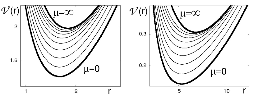
Figure 2: Potentials , in
, versus , in . Left panel:
[]; right panel
[]. Thick lines: spherical harmonic oscillator (),
and harmonium (). Thin lines: ,
, . The horizontal lines
correspond to , i.e. to .Figure 3: Ratio of potentials of erfonium and harmonium versus
(in ) for (left panel) and for (right panel).
Thick lines - ; thin lines - . The lines are marked
by the values of . If then the lines
corresponding to different overlap.
Plots of for and for are
shown in Fig. 2. As one can see, the curves correspnding to large are
close to the potential of harmonium and the ones corresponding to small
to the potential of the spherical harmonic oscillator. The shapes of the
left- and of the right-panel potentials ( and , respectively),
are the same, but the ranges of units differ by the scaling factor
.
Similarities and differences between erfonium and harmonium potentials
are well reflected by their ratio:
(36)
If then, for given and , the ratio is an increasing
function of . At the limit of , or ,
or , the ratio is equal to . If ,
or , then = 0. Plots of versus , for
several values of and are shown in the left panel of Fig. 3.
As one can see, the -dependence is essential for
small values of only. One can also notice a fast convergence of
to with increasing .
III The effective potential
The shape of , similarly as the shape of
, is conserved under some specific transformations.
Equation (11) can be rewritten as
(37)
where . Then,
(38)
if
(39)
[compare eq. (21)]. This means, that two effective potentials have the
same shape if,
(40)
Figure 4: The effective potential
(in )
for , as functions of the inter-electronic distance
(in ). Left panel - ; right panel - .
The lowest curves represent the effective potentials of the spherical
harmonic oscillator (), and the upper ones of harmonium ().
The curves between these two limits correspond to (left),
and (right), for .
are, respectively, the effective potentials of harmonium and of the
spherical harmonic oscillator.
Since , we have
(44)
The general shapes of and
are similar: regular potential wells
approaching infinity in the same way if and
. Because is regular and monotonic,
the shapes of are similar.
In Fig. 4 plots of for ,
(left panel), , (right panel), and
for several values of are presented.
The ranges of and in the two panels are selected so
that the shapes of the curves are similar [the shapes cannot be the same,
because , cf. eq. (39)].
Figure 5: Plots of the normalized coordinates of the minimum of the effective
potential for and – curves , , ,
respectively, as functions of . In the left panel
; in the
right one .
If then the effective potential
has only one extremum: a minimum, at .
The values of can be obtained from the condition
transformed to
(45)
where stands here for ). Equation (45)
has to be solved numerically, but one can see that
), if
. At the limit of
(harmonic oscillator),
(46)
If (harmonium), then is a root of a
fourth-order polynomial:
(47)
The explicit expression is given in Mandal et al. (2003).
The second coordinate of this minimum is
,
The normalized coordinates of the minimum,
(48)
are plotted versus in, respectively, left and right
panels of Fig. 5. Similarly as in the
case of the model potential (cf. Fig. 1) the minimum of the
effective potential is approximately located at its asymptotic
position already for . But, unlike the case
of , here both
and depend
on .
Finally, the ratio
(49)
for , and for several values of and is plotted
in the right panel of Fig. 3. As in the case of
, the -dependence is noticeable for small values of
only. The differences between the effective potentials for finite
values of , and their asymptotic forms is, in the case of ,
much smaller than for . This can be seen in Fig. 3: the
maximum difference between and is about three times smaller
than between 1 and .
IV Spectrum
Figure 6: Plots of [eq. (53)] expressed in
versus (in ) for
(top panels) and
(bottom panels); (left panels) and (right panels).
The vertical lines mark ; the tangent lines in the
bottom-left corners of the panels and the horizontal lines in the upper parts
of the panels show the asymptotic behavior of for
and , respectively. The upper
curves (marked ) correspond to the ground states and the lowest ones
(marked ) - to the fifth excited states.
At the energy spectrum is given by the well known analytic formula
(50)
According to the Hellmann-Feynman theorem,
(51)
Therefore, for a fixed , and ,
(52)
Differences
(53)
for , , and for two values of
differing by factor (, and ) are
plotted, as functions of , in Fig. 6. Though the scaling invariance
discussed in previous sections is not valid exactly, one can see that the
spectra for different values of the confinement parameter have similar
structure.
The average distance between electrons, , in the case of
the harmonic oscillator, is proportional to .
This kind of dependence is approximately valid for a broad range of .
The increasing repulsion between electrons (increasing ) leads
to an increase of . In the case of the
average distance between electrons is of the order of ,
increasing from about at the limit of the harmonic
oscillator to at the limit of harmonium. In such cases
the influence of the centrifugal term, proportional to , is
small – for small the wave function is close to .
This can be seen by comparing the left and the right
panels in Fig. 6: a difference is visible if , but
if , then the plots for and for are nearly
the same – the relative difference between the ground state energies
of and is, in the case of , about .
The range of the validity of the linear approximation (52)
can be estimated for small by comparing the tangent lines
(54)
with the curves representing the exact energies.
Figure 7: Plots of [eq. (55)] expressed in
versus (in ) for .
Left panel: ; right panel: .
The vertical lines mark . The curves (marked ) correspond to
the ground state and the ones marked - to the fifth excited state.
The energy of harmonium can be expressed analytically only in some
special cases, but the structure of its spectrum is well known
(see e.g. Karwowski and Cyrnek (2004)). As a function of , the spectrum
can be divided to three parts:
(1) – strong confinement dominates the Coulomb interaction,
the electron correlation is weak and we have the harmonic oscillator regime;
(2) – the
intermediate regime, the relation between the confinement and the Coulomb
interaction is, in a sense, similar as in atoms; (3) –
very weak confinement, the electrons are far apart and their motion is
strongly correlated. Differences
(55)
for , , and are
plotted, as functions of , in Fig. 7. Similarly as in the diagrams
presented in Fig. 6, also here one can see a qualitative change of the
spectrum when . In the case of the
harmonic oscillator the distances between the neighboring energy
levels, for given and , are constant (independent of ).
In the case of harmonium, these distances increase with increasing
Karwowski and Cyrnek (2004). When changes from the large to the small values,
the distances between the energy levels gradually change from the mode of
harmonium to the mode of harmonic oscillator. This can be seen in Fig. 7 –
in the area , the order of the values of
in terms of , changes to the reverse.
Figure 8: Plots of [eq. (56)] expressed in
versus (in ), for
(left panel) and (right panel), and . The vertical
lines mark . The curves marked correspond to the ground
state and the ones marked - to the fifth excited state.
As it was already mentioned, using the smooth long-range interaction
potential instead of the singular Coulomb one, reduces the computational
effort in the approximate solving the Schrödinger equation for
many-electron systems Gori-Giorgi and Savin (2006); Savin (2011, 2020). Therefore, one of the
objectives of studying properties of erfonium, is an exploration
of the possibility of an extrapolation of the energy derived from a model
with a finite to the limit of electrons interacting by the Coulomb
force, i.e. the transition from the spectrum of a finite- erfonium to
the spectrum of harmonium. The first step in such a procedure is the
approximation of the energies of harmonium by the expectation values of
the harmonium Hamiltonian calculated using the wave functions of erfonium
Savin and Karwowski (2023). The resulting correction to the energy, equal to
(56)
where
is plotted in Fig. 8. As one can see by comparing with Fig. 7, the
difference between and
depends on the value of .
If is large (left panels), then
(for
by factor ). But if is small (right
panels), then both differences are of the same order of magnitude.
The difference between and
can be dramatically reduced if the generalized
cusp conditions are used to represent the wave function at small .
But, if is smaller than a certain threshold, a further reduction of
the difference using this method proved to be impossible Savin and Karwowski (2023).
From the perspective of the present analysis it is understandable that
the threshold value is close to , where the character of the
potential (and of the spectrum) changes from a harmonium-like to an
oscillator-like.
V Final remarks
Erfonium, a Hooke atom with a soft interaction potential
represented by , makes a bridge between harmonium
() and the spherical harmonic oscillator ().
The parameter establishes an adiabatic connection between these
two limits. An interplay between the effects specific for harmonium and
for the harmonic oscillator creates a rich and interesting pattern which
can be observed in the structure of the potential and of the spectrum.
The parameter determined by the strength of the confinement
(27), marks a fuzzy boundary between these two ”spheres of influence”.
If then the regime of harmonium dominates, if
, then the features of the harmonic oscillator prevail.
A vast field for further studies remains open. Particularly interesting (and
difficult) are issues related to the behavior of erfonium at the limit
of . Notice that at this limit the spectrum abruptly
changes from entirely discrete, to entirely continuous. If simultaneously
, then at the limit we get two unconfined and
non-interacting ’electrons’.
Last, but not least, a broad class of semi-analytic (cf.
Taut (1993); Mandal et al. (2003)) and variational approaches may result in precise
analytic approximations of the wave functions and of the energies of erfonium.
Acknowledgement
We thank Prof. Henryk A. Witek (National Chiao Tung University, Hsinchu,
Taiwan) for his constructive remarks and for useful discussions.
ORCID
Jacek Karwowski: https://orcid.org/0000-0003-1508-2929
Andreas Savin: https://orcid.org/0000-0001-8401-8037
References
Gori-Giorgi and Savin (2006)P. Gori-Giorgi and A. Savin, “Properties of
short-range and long-range correlation energy density functionals from
electron-electron coalescence,” Phys.
Rev. A 73, 032506
(2006).
Savin (2011)A. Savin, “Correcting model
energies by numerically integrating along an adiabatic connection and a link
to density functional approximations,” J. Chem. Phys. 134, 214108 (2011).
Savin (2020)A. Savin, “Models and
corrections: Range separation for electronic interaction – Lessons from
density functional theory,” J. Chem. Phys. 153, 160901 (2020).
Savin and Karwowski (2023)A. Savin and J. Karwowski, “Correcting
models with long-range electron interaction using generalized cusp
conditions,” J. Phys. Chem. A 127, 1377–1385 (2023).
González-Espinoza et al. (2016)C. E. González-Espinoza, P. W. Ayers, J. Karwowski, and A. Savin, “Smooth models for the coulomb
potential,” Theor. Chem. Acc. 135, 256 (2016).
Pernal and Hapka (2022)K. Pernal and M. Hapka, “Range-separated
multiconfigurational density functional theory methods,” WIREs Comput.
Mol. Sci. 12, e1566
(2022).
Ewald (1921)P. P. Ewald, “Die berechnung
optischer und elektrostatischer gitterpotentiale (the calculation of optical
and electrostatic grid potential),” Ann.
Phys (Leipzig) 369, 253–287 (1921).
Lucha et al. (1992)W. Lucha, H. Rupprecht, and F. F. Schoeberl, “Significance of relativistic
wave equations for bound states,” Phys.
Rev. D 46, 1088–1095
(1992).
Kestner and Sinanoglu (1962)N. R. Kestner and O. Sinanoglu, “Study of
electron correlation in helium-like systems using an exactly soluble
model,” Phys. Rev. 128, 2687 (1962).
Taut (1993)M. Taut, “Two electrons in
an external oscillator potential: Particular analytic solutions of a coulomb
correlation problem,” Phys. Rev. A 48, 3561–3566 (1993).