Convex envelopes of bounded monomials on two-variable cones

Abstract.

We consider an $n$-variate monomial function that is restricted both in value by lower and upper bounds and in domain by two homogeneous linear inequalities. Such functions are building blocks of several problems found in practical applications, and that fall under the class of Mixed Integer Nonlinear Optimization. We show that the upper envelope of the function in the given domain, for $n\geq 2$ is given by a conic inequality. We also present the lower envelope for $n=2$. To assess the applicability of branching rules based on homogeneous linear inequalities, we also derive the volume of the convex hull for $n=2$.

1. Introduction

Consider the function $f:\mathbb{R}_{+}^{n}\to\mathbb{R}_{+}$ defined as $f({\boldsymbol{x}})=\prod_{i\in N}x_{i}^{a_{i}}$ where $N=\{1,2,\ldots{},n\}$, $n>1$, $a_{i}>0\forall i\in N$. We are interested in the convex envelope of $f$ on subsets of $\mathbb{R}_{+}^{n}$ where the value of $f$ itself is bounded in the range $[\ell,u]$, with $0<\ell<u<+\infty$. Specifically, for a given $\mathcal{D}\subseteq\mathbb{R}_{+}^{n}$ we seek the convex hull of the set $F(\mathcal{D})=\{({\boldsymbol{x}},z)\in(X\cap\mathcal{D})\times\mathbb{R}:z=f({\boldsymbol{x}})\}$, where

$$X=\{{\boldsymbol{x}}\in\mathbb{R}_{+}^{n}:\ell\leq f({\boldsymbol{x}})\leq u\}.$$

Finding or approximating the convex hull of $F(\mathcal{D})$ is useful in solving optimization problems whose objective function or constraints contain polynomials with arbitrary real exponents. In particular, those monomials with variables restricted to the first orthant are of interest in the optimization with posynomial functions, or, more in general, in geometric programming [9, 10]. Some algorithms for posynomial optimization and for providing relaxations and lower bounds for monomials on positive variables have been proposed [15, 29].

Monomials also appear in optimization problems with general nonlinear constraints and discrete variables. Mixed-Integer Nonlinear Optimization (MINLO) solvers such as Antigone [18], Baron [22], Couenne [4], SCIP [8], and FICO-Xpress [11] employ a reformulation scheme where expressions in factorable programs are decomposed to smaller expressions that can be targeted by an operator-specific convexification algorithm [23, 28]. This allows for exploiting branch-and-bound algorithms to compute the global optimum of a MINLO problem [12]. For instance, the generic polynomial constraint

(1) $$\sum_{j\in J}c_{j}\prod_{i\in I_{j}}x_{i}^{a_{ji}}\leq c_{0},$$

where $c_{j}\in\mathbb{R}$, $a_{ji}\in\mathbb{R}$, and $c_{0}\in\mathbb{R}$, is in general nonconvex, and is decomposed by introducing auxiliary variables $y_{j}$ and $t_{ji}$ as follows:

(2) $$\sum_{j\in J}c_{j}y_{j}\leq c_{0}$$

(3) $$y_{j}=\prod_{i\in I_{j}}t_{ji} \forall j\in J$$

(4) $$t_{ji}=x_{i}^{a_{ji}} \forall i\in I_{j},\forall j\in J.$$

Exact solvers like those mentioned above find or approximate the convex hull of the sets defined by the constraints associated with each of the auxiliary variables. A convex relaxation of the feasible set for (2)-(4), which yields a valid lower bound for the MINLO problem, is

$$\textstyle R=R^{\prime}\cap\left(\bigcap_{j\in J}R^{\prime\prime}_{j}\right)\cap\left(\bigcap_{j\in J,i\in I_{j}}R^{\prime\prime\prime}_{ji}\right),$$

where

$$\begin{array}[]{lll}R^{\prime}&=&\{({\boldsymbol{x}},{\boldsymbol{w}},{\boldsymbol{t}}):\sum_{j\in J}c_{j}y_{j}\leq b\},\\ R^{\prime\prime}_{j}&\supseteq&\textrm{conv}\left(\left\{({\boldsymbol{x}},{\boldsymbol{w}},{\boldsymbol{t}}):y_{j}=\prod_{i\in I_{j}}t_{ji}\right\}\right),\\[5.69054pt] R^{\prime\prime\prime}_{ji}&\supseteq&\textrm{conv}\left(\left\{({\boldsymbol{x}},{\boldsymbol{w}},{\boldsymbol{t}}):t_{ji}=x_{i}^{a_{ji}}\right\}\right).\end{array}$$

Clearly $R^{\prime}$ is defined by a linear constraint and is added to the reformulation as is. The reformulation results in a lower bound on the optimal objective value that is tighter when $R^{\prime\prime}_{j}$ and $R^{\prime\prime\prime}_{ji}$ are tight approximations of the corresponding convex hulls. Note that even in the case $R^{\prime\prime}$ and $R^{\prime\prime\prime}$ are equal to, rather than supersets of, the corresponding convex hulls, $R$ is still in general not the convex hull of the set described by (2)-(4). The tightness of such relaxations strongly depends on tight bounds on both the original variables $x_{i}$ and the auxiliaries $y_{j}$ and $t_{ji}$. Several bound reduction techniques such as feasibility-based (see e.g. Neumeier [19]) and optimality-based [28] help find tight bounds on all auxiliary variables. Before generating an LP relaxation for (1), most solvers apply bound reduction to find a tight bound interval $[\ell_{j},u_{j}]$ on $y_{j}$ and $[\ell_{ji},u_{ji}]$ on $t_{ji}$. This motivates the search for convex envelopes of $f$ over $X\cap\mathcal{D}$.

The equality signs in (3) and (4) can be relaxed depending on the sign of $c_{j}$, which may render (4) convex depending on $a_{ji}$: if $a_{ji}\geq 1$, then the constraint $t_{ji}\geq x_{i}^{a_{ji}}$ is convex, and viceversa if $a_{ji}\leq 1$ then $t_{ji}\leq x_{i}^{a_{ji}}$ is convex.

However, (3) is nonconvex regardless of the sign, although it admits a polyhedral convex hull [21]. McCormick [16] provides a valid relaxation for the product of two variables,

(5) $$B=\{(x_{1},x_{2},z)\in\mathbb{R}^{3}_{+}:z=x_{1}x_{2},(x_{1},x_{2})\in[\ell_{1},u_{1}]\times[\ell_{2},u_{2}]\},$$

which consists of the four so-called McCormick inequalities:

(6) $$z \geq \ell_{2}x_{1}+\ell_{1}x_{2}-\ell_{2}\ell_{1}$$

(7) $$z \geq u_{2}x_{1}+u_{1}x_{2}-u_{2}u_{1}$$

(8) $$z \leq \ell_{2}x_{1}+u_{1}x_{2}-\ell_{2}u_{1}$$

(9) $$z \leq u_{2}x_{1}+\ell_{1}x_{2}-u_{2}\ell_{1}.$$

These inequalities, in fact, form the convex hull of $B$ [2]. While these results hold without sign constraints on $x_{1}$ and $x_{2}$, we use the above definition of $B$ as we focus on sets entirely contained in $\mathbb{R}_{+}^{n}$. Meyer and Floudas [17] present inequalities of the convex hull in the trilinear case ($n=3$).

1.1. The case for bounded monomials

Bound reduction that uses the bounds on the initial variables ${\boldsymbol{x}}$ and the linear constraint (2) can obtain, as an implication, lower and upper bound on each element of the sum in (1). In the bilinear case, i.e., $n=2$, $a_{1}=a_{2}=1$, the convex hull of

$$B^{\prime}=\{(x_{1},x_{2},z)\in B:\ell\leq z\leq u\}$$

is tighter than (6)-(9) if the bounds on $z$ are tighter than those on $x_{1}$ and $x_{2}$, i.e., $\ell>\ell_{1}\ell_{2}$ or $u<u_{1}u_{2}$.

Belotti et al. [6] introduce inequalities that are not implied by the McCormick inequalities if at least one of the bounds on $z$ is tighter, and that result in a tighter relaxation when solving quadratically constrained MINLO problems. Anstreicher et al. [3] show that the convex hull of $B^{\prime}$ for “tight” values of $\ell$ or $u$ is the union of distinct regions, each partially delimited by a different second-order cone, i.e., a set of the form ${\boldsymbol{b}}^{\top}{\boldsymbol{x}}+b_{0}\geq\|G{\boldsymbol{x}}+{\boldsymbol{g}}\|_{2}$. Nguyen et al. [20] obtain envelopes of monomials $x_{1}^{a_{1}}x_{2}^{a_{2}}$ for the cases $a_{1}=1\leq a_{2}$ (convex hull and upper envelope) and $a_{1},a_{2}\geq 1$ (lower envelope).

This article mainly focuses on the convex hull of $F(\mathcal{D})$ where

(10) $$\mathcal{D}=W_{ij}:=\{{\boldsymbol{x}}\in\mathbb{R}_{+}^{n}:px_{i}\leq x_{j}\leq qx_{i}\},$$

with $0<p<q$, for two indices $i,j\in N$. Therefore we depart from the most usual setting where lower and upper bounds on ${\boldsymbol{x}}$ are given, and instead constrain the ${\boldsymbol{x}}$ variables with two homogeneous (i.e. zero right-hand side) linear inequalities, which restrict the ${\boldsymbol{x}}$ space to a wedge.

Using linear inequalities instead of a bounding box as the feasible set for ${\boldsymbol{x}}$ deviates from the common setting exploited by MINLO solvers. An advantage of this approach is that we may obtain a tighter relaxation by avoiding the decomposition of the factorable term $\prod_{i\in N}x_{i}^{a_{i}}$ into $y=\prod_{i\in N}t_{i}$ and $t_{i}=x_{i}^{a_{i}}$.

While we assume $a_{i}>0\forall i\in N$, note that we can reduce monomials with one or more terms $x_{i}^{a_{i}}$ with $a_{i}<0$ to this case by another reformulation step: introduce an auxiliary variable $y_{i}$ such that $y_{i}=\frac{1}{x_{i}}$ and replace $x_{i}^{a_{i}}$ with $y_{i}^{-a_{i}}$. This requires $x_{i}>0\forall{\boldsymbol{x}}\in X\cap\mathcal{D}$, which is implied by $\ell>0$, and it introduces an extra gap due to the additional reformulation step $\{(x_{i},y_{i})\in\mathbb{R}_{+}^{2}:x_{i}y_{i}=1\}$, whose convex hull is $\{(x_{i},y_{i})\in\mathbb{R}_{+}^{2}:x_{i}y_{i}\geq 1\}$ if $x_{i}\in[0,+\infty]$, otherwise it is $\{(x_{i},y_{i})\in\mathbb{R}_{+}^{2}:x_{i}y_{i}\geq 1,x_{i}+u\ell y_{i}\leq\ell+u\}$.

Definition 1.

Given $T\subseteq\mathbb{R}^{n}$ and a function $f:T\to\mathbb{R}$, the epigraph of $f$ in $T$ is $\textrm{epi}(f,T)=\{({\boldsymbol{x}},z)\in T\times\mathbb{R}:z\geq f({\boldsymbol{x}})\}$. The hypograph of $f$ in $T$ is $\textrm{hyp}(f,T)=\{({\boldsymbol{x}},z)\in T\times\mathbb{R}:z\leq f({\boldsymbol{x}})\}$.

Definition 2.

Given $T\subseteq\mathbb{R}^{n}$ and a function $f:T\to\mathbb{R}$, the lower envelope $E_{L}(f,T)$ (resp. upper envelope $E_{U}(f,T)$) of $f$ over $T$ is the convex hull of the epigraph (resp. hypograph) of $f$ in $T$.

In Section 2 we provide some trivial results on the convex hull of $F(\mathbb{R}_{+}^{n})$. In Section 3 we present the upper envelope of $f$ over $X\cap W_{ij}$ for any $n\geq 2$. In Section 4 we present the lower envelope of $f$ over $X\cap W_{ij}$ for $n=2$, yielding the convex hull of $F(W_{12})$. In Section 5 we compute the volume of the convex hull of $F(W_{12})$ for $n=2$; concluding remarks are in Section 6.

2. Convex hull of $F(\mathbb{R}_{+}^{n})$

Define $\beta=\sum_{i\in N}a_{i}$, then for $z_{0},\gamma\in\mathbb{R}$ consider the cone

$$\textstyle\mathcal{K}=\left\{({\boldsymbol{x}},z)\in\mathbb{R}_{+}^{n}\times\mathbb{R}:(z-z_{0})^{\beta}\leq\gamma\prod_{i\in N}x_{i}^{a_{i}}\right\}.$$

The vertex of $\mathcal{K}$ is $({\mathbf{0}},z_{0})$. Also define $F(\mathcal{D})^{\leq}:=\{({\boldsymbol{x}},z)\in(X\cap\mathcal{D})\times\mathbb{R}:z\leq f({\boldsymbol{x}})\}$; note that it is obviously not the hypograph of $f$ but rather a relaxation of the link between $z$ and $f$. If $\beta=1$ then $F(\mathcal{D})^{\leq}$ is a convex cone intersected with $S:=\{({\boldsymbol{x}},z)\in\mathbb{R}_{+}^{n}\times\mathbb{R}:\ell\leq z\leq u\}=\mathbb{R}_{+}^{n}\times[\ell,u]$. Similar to the bilinear case, where $n=2$ and $a_{1}=a_{2}=1$, we look for conditions under which $\mathcal{K}$ defines a tight relaxation of $F(\mathcal{D})$. Let us find $z_{0}$ and $\gamma$ such that

$$\begin{array}[]{ll}\{({\boldsymbol{x}},z)\in F(\mathcal{D})^{\leq}:z=\ell\}=\{({\boldsymbol{x}},z)\in\mathcal{K}:z=\ell\};\\ \{({\boldsymbol{x}},z)\in F(\mathcal{D})^{\leq}:z=u\}=\{({\boldsymbol{x}},z)\in\mathcal{K}:z=u\}.\end{array}$$

This is equivalent to finding $z_{0},\gamma$ such that

(11) $$\begin{array}[]{ll}\ell\leq\prod_{i\in N}x_{i}^{a_{i}}\Leftrightarrow\frac{1}{\gamma}(\ell-z_{0})^{\beta}\leq\prod_{i\in N}x_{i}^{a_{i}}&\forall{\boldsymbol{x}}\in\mathbb{R}_{+}^{n};\\[2.84526pt] u\leq\prod_{i\in N}x_{i}^{a_{i}}\Leftrightarrow\frac{1}{\gamma}(u-z_{0})^{\beta}\leq\prod_{i\in N}x_{i}^{a_{i}}&\forall{\boldsymbol{x}}\in\mathbb{R}_{+}^{n}\\ \end{array}$$

and hence $\ell=\frac{1}{\gamma}(\ell-z_{0})^{\beta},u=\frac{1}{\gamma}(u-z_{0})^{\beta}$, which implies $z_{0}\leq\ell$. Because $u>0$ and $u-z_{0}>0$, we divide the first equation by the second one and obtain $\left(\frac{\ell}{u}\right)^{1/\beta}=\frac{(\ell-z_{0})}{(u-z_{0})}$. This yields

(12) $$z_{0}=\frac{u^{\frac{1}{\beta}}\ell-\ell^{\frac{1}{\beta}}u}{u^{\frac{1}{\beta}}-\ell^{\frac{1}{\beta}}},\quad\gamma=\left(\frac{u-\ell}{u^{\frac{1}{\beta}}-\ell^{\frac{1}{\beta}}}\right)^{\beta}.$$

Note that $\beta\geq 1\Leftrightarrow(z_{0}\leq 0,\gamma\geq 1)$. Also, if $\beta=1$, $z_{0}=0$, $\gamma=1$, and it is easy to verify that $\mathcal{K}\cap S\equiv F(\mathbb{R}_{+}^{n})^{\leq}$, while $\ell=0$ implies $z_{0}=0$, i.e., the vertex of $\mathcal{K}$ is the origin.

Lemma 1.

For $a_{i}>0\forall i\in N$, $\ell\geq 0$, $T=\{{\boldsymbol{x}}\in\mathbb{R}_{+}^{n}:\prod_{i\in N}x_{i}^{a_{i}}\geq\ell\}$ is convex.

Proof.

If $\ell=0$, $T=\mathbb{R}_{+}^{n}$. Assume now $\ell>0$; then $x_{i}>0,i\in N$, for all ${\boldsymbol{x}}\in T$. Consider ${\boldsymbol{x}}^{\prime},{\boldsymbol{x}}^{\prime\prime}\in T$. For any $\mu\in[0,1]$, we prove $\prod_{i\in N}(\mu x^{\prime}_{i}+(1-\mu)x^{\prime\prime}_{i})^{a_{i}}\geq\ell$, i.e.,

$$\sum_{i\in N}a_{i}\log\left(\mu x^{\prime}_{i}+(1-\mu)x^{\prime\prime}_{i}\right)\geq\log\ell.$$

Concavity of the $\log$ function and positivity of all $a_{i}$’s imply

$$\begin{array}[]{ll}&\sum_{i\in N}a_{i}\log\left(\mu x^{\prime}_{i}+(1-\mu)x^{\prime\prime}_{i}\right)\geq\\ \geq&\sum_{i\in N}a_{i}(\mu\log x^{\prime}_{i}+(1-\mu)\log x^{\prime\prime}_{i})=\\ =&\mu\sum_{i\in N}a_{i}\log x^{\prime}_{i}+(1-\mu)\sum_{i\in N}a_{i}\log x^{\prime\prime}_{i}\geq\\ \geq&\mu\log\ell+(1-\mu)\log\ell=\log\ell,\end{array}$$

which proves convexity of $T$. ∎

Lemma 2.

Let $g:\mathbb{R}\to\mathbb{R}$ be a convex (resp. concave) monotone non-decreasing function. Then for any $\ell,z,u$ such that $\ell<z<u$,

$$\frac{g(z)-g(\ell)}{z-\ell}\leq\frac{g(u)-g(z)}{u-z}\qquad\left(\textrm{resp. }\frac{g(z)-g(\ell)}{z-\ell}\geq\frac{g(u)-g(z)}{u-z}\right).$$

Proof.

Consider $\mu\in(0,1)$ such that $z=(1-\mu)\ell+\mu u$. Then $0<\mu<1$ and for $g$ concave we obtain $g(z)\geq(1-\mu)g(\ell)+\mu g(u)$, or

$$\begin{array}[]{rcl}(1-\mu)g(z)+\mu g(z)&\geq&(1-\mu)g(\ell)+\mu g(u)\\ (1-\mu)z+\mu z&=&(1-\mu)\ell+\mu u\\[5.69054pt] (1-\mu)(g(z)-g(\ell))&\geq&\mu(g(u)-g(z))\\ (1-\mu)(z-\ell)&=&\mu(u-z).\\ \end{array}$$

Dividing the third inequality by the last equation yields $\frac{g(z)-g(\ell)}{z-\ell}\geq\frac{g(u)-g(z)}{u-z}$. Similar considerations hold, mutatis mutandis, for $g$ convex. ∎

Lemma 3.

$F(\mathbb{R}_{+}^{n})\subseteq\mathcal{K}$ if and only if $\beta\geq 1$.

Proof.

$F(\mathbb{R}_{+}^{n})\subseteq\mathcal{K}$ if and only if $(\ell\leq z\leq u)\wedge(z=\prod_{i\in N}x_{i}^{a_{i}})\Rightarrow(z-z_{0})^{\beta}\leq\gamma\prod_{i\in N}x_{i}^{a_{i}}$. Rewrite the left-hand side as $(z-z_{0})^{\beta}\leq\gamma z$. Replacing $z_{0}$ and $\gamma$ we get

$$\left(z-\frac{u^{1/\beta}\ell-\ell^{1/\beta}u}{u^{1/\beta}-\ell^{1/\beta}}\right)^{\beta}\leq\left(\frac{u-\ell}{u^{1/\beta}-\ell^{1/\beta}}\right)^{\beta}z,$$

from which we eliminate the (positive) common denominator:

$$\begin{array}[]{lcll}&\textstyle\left(zu^{\frac{1}{\beta}}-z\ell^{\frac{1}{\beta}}-u^{\frac{1}{\beta}}\ell+\ell^{\frac{1}{\beta}}u\right)^{\beta}&=\\ =&\textstyle\left(u^{\frac{1}{\beta}}(z-\ell)+\ell^{\frac{1}{\beta}}(u-z)\right)^{\beta}&\leq&\textstyle(u-\ell)^{\beta}z.\end{array}$$

Because $\beta>0$ and all terms in both left- and right-hand side are nonnegative, the above is equivalent to

(13) $$u^{\frac{1}{\beta}}(z-\ell)+\ell^{\frac{1}{\beta}}(u-z)\leq(u-\ell)z^{\frac{1}{\beta}}.$$

Rewrite the right-hand side as $(u-z)z^{\frac{1}{\beta}}+(z-\ell)z^{\frac{1}{\beta}}$ and (13) as $(u-z)(z^{\frac{1}{\beta}}-\ell^{\frac{1}{\beta}})\geq(z-\ell)(u^{\frac{1}{\beta}}-z^{\frac{1}{\beta}})$, or

$$\frac{z^{\frac{1}{\beta}}-\ell^{\frac{1}{\beta}}}{z-\ell}\geq\frac{u^{\frac{1}{\beta}}-z^{\frac{1}{\beta}}}{u-z},$$

which, for Lemma 2, is true if and only if $\beta\geq 1$ for concavity of $g(x)=x^{\frac{1}{\beta}}$. ∎

The structure of both upper envelope and lower envelope of $f$ over $X\cap\mathcal{D}$ discussed in this and the following section changes radically at $\beta=1$. For instance, $F(\mathbb{R}_{+}^{n})^{\leq}$ is convex for $\beta\leq 1$ and nonconvex for $\beta>1$. Therefore we split the treatment within each section depending on the ranges of $\beta$.

Proposition 1.

If $\beta\geq 1$, then $\textrm{conv}(F(\mathbb{R}_{+}^{n}))=\mathcal{K}\cap S$.

Proof.

$F(\mathbb{R}_{+}^{n})\subseteq\mathcal{K}$ from Lemma 3; this implies that $\textrm{conv}(F(\mathbb{R}_{+}^{n}))\subseteq\mathcal{K}$ as $\mathcal{K}$ is convex. In addition, $F(\mathbb{R}_{+}^{n})\subseteq S$ and convexity of $S$ imply $\textrm{conv}(F(\mathbb{R}_{+}^{n}))\subseteq\mathcal{K}\cap S$. We just need to prove $\textrm{conv}(F(\mathbb{R}_{+}^{n}))\supseteq\mathcal{K}\cap S$.

Consider $(\tilde{\boldsymbol{x}},\tilde{z})\in\mathcal{K}\cap S$, i.e., $(\tilde{z}-z_{0})^{\beta}\leq\gamma\prod_{i\in N}\tilde{x}_{i}^{a_{i}}$, $\ell\leq\tilde{z}\leq u$. Let us construct ${\boldsymbol{x}}^{\prime}$ and ${\boldsymbol{x}}^{\prime\prime}$ such that $(\tilde{\boldsymbol{x}},\tilde{z}-z_{0})$ is a convex combination of $({\boldsymbol{x}}^{\prime},\ell-z_{0})$ and $({\boldsymbol{x}}^{\prime\prime},u-z_{0})$. Let $({\boldsymbol{x}}^{\prime},\ell-z_{0})=s^{\prime}(\tilde{\boldsymbol{x}},\tilde{z}-z_{0})$ and $({\boldsymbol{x}}^{\prime\prime},u-z_{0})=s^{\prime\prime}(\tilde{\boldsymbol{x}},\tilde{z}-z_{0})$, i.e., $({\boldsymbol{x}}^{\prime},\ell)$ and $({\boldsymbol{x}}^{\prime\prime},u)$ lie on the same ray of $\mathcal{K}$ as $(\tilde{\boldsymbol{x}},\tilde{z})$. By construction of $s^{\prime}$ and $s^{\prime\prime}$,

$$s^{\prime}=\frac{\ell-z_{0}}{\tilde{z}-z_{0}}\leq 1;\qquad s^{\prime\prime}=\frac{u-z_{0}}{\tilde{z}-z_{0}}\geq 1.$$

In addition, $({\boldsymbol{x}}^{\prime},\ell)\in\mathcal{K}$ and $({\boldsymbol{x}}^{\prime\prime},u)\in\mathcal{K}$ because $(\tilde{\boldsymbol{x}},\tilde{z})\in\mathcal{K}$. Specifically, they belong to $\{({\boldsymbol{x}},z)\in\mathcal{K}:z=\ell\}$ and $\{({\boldsymbol{x}},z)\in\mathcal{K}:z=u\}$, respectively, but by (11) this implies $({\boldsymbol{x}}^{\prime},\ell)\in F^{\leq}_{\ell}:=\{({\boldsymbol{x}},z)\in F(\mathbb{R}_{+}^{n})^{\leq}:z=\ell\}$ and $({\boldsymbol{x}}^{\prime\prime},u)\in F^{\leq}_{u}:=\{({\boldsymbol{x}},z)\in F(\mathbb{R}_{+}^{n})^{\leq}:z=u\}$. Because both $F^{\leq}_{\ell}$ and $F^{\leq}_{u}$ are convex by Lemma 1, there exist two extreme points ${\boldsymbol{x}}^{\prime}_{a}$ and ${\boldsymbol{x}}^{\prime}_{b}$ of $F(\mathbb{R}_{+}^{n})$ of which ${\boldsymbol{x}}^{\prime}$ is a convex combination, such that $f({\boldsymbol{x}}^{\prime}_{a})=f({\boldsymbol{x}}^{\prime}_{b})=\ell$, and similar for ${\boldsymbol{x}}^{\prime\prime}$, thus implying $(\tilde{\boldsymbol{x}},\tilde{z})$ is a convex combination of points of $F(\mathbb{R}_{+}^{n})$. ∎

Proposition 2.

If $\beta\leq 1$, then $\textrm{conv}(F(\mathbb{R}_{+}^{n}))=F(\mathbb{R}_{+}^{n})^{\leq}$.

Proof.

$F(\mathbb{R}_{+}^{n})\subseteq F(\mathbb{R}_{+}^{n})^{\leq}$ and $F(\mathbb{R}_{+}^{n})^{\leq}$ is convex, therefore $\textrm{conv}(F(\mathbb{R}_{+}^{n}))\subseteq F(\mathbb{R}_{+}^{n})^{\leq}$. To prove $\textrm{conv}(F(\mathbb{R}_{+}^{n}))\supseteq F(\mathbb{R}_{+}^{n})^{\leq}$, consider $(\tilde{\boldsymbol{x}},\tilde{z})\in F(\mathbb{R}_{+}^{n})^{\leq}$. If $f(\tilde{\boldsymbol{x}})=\tilde{z}$, obviously the result holds. If $\tilde{z}<f(\tilde{\boldsymbol{x}})$, similar to the proof of Proposition 1, convexity of $T=\{({\boldsymbol{x}},z)\in F(\mathbb{R}_{+}^{n})^{\leq}:z=\tilde{z}\}$ implies there exist two extreme points of $T$, i.e., two elements of $\{({\boldsymbol{x}},z)\in F(\mathbb{R}_{+}^{n}):z=\tilde{z}\}$, of which $(\tilde{\boldsymbol{x}},\tilde{z})$ is a convex combination. ∎

3. Upper envelope over $X\cap W_{ij}$

We established that the convex hull of $F(\mathbb{R}_{+}^{n})$ is defined by $\mathcal{K}\cap S$ if $\beta\geq 1$ and $F(\mathbb{R}_{+}^{n})^{\leq}$ otherwise. From now on, we consider $\mathcal{D}=W_{ij}$ defined in (10):

$$W_{ij}=\{{\boldsymbol{x}}\in\mathbb{R}_{+}^{n}:px_{i}\leq x_{j}\leq qx_{i}\}.$$

Below we prove that the above result on the upper envelope is substantially unchanged, save an extra inequality for $n=2$.

Lemma 4.

For any $0<p\leq q<+\infty$, the set $X\cap W_{ij}$ is bounded for $n=2$ and unbounded for $n>2$.

Proof.

For $n=2$, $x_{1}^{a_{1}}x_{2}^{a_{2}}\leq u$ and $x_{2}\geq px_{1}$ imply $p^{a_{2}}x_{1}^{a_{1}+a_{2}}\leq x_{1}^{a_{1}}x_{2}^{a_{2}}\leq u$, i.e., $x_{1}\leq\omega_{1}:=(up^{-a_{2}})^{\frac{1}{a_{1}+a_{2}}}$. Similarly, $x_{1}^{a_{1}}x_{2}^{a_{2}}\leq u$ and $x_{2}\leq qx_{1}$ imply $q^{-a_{1}}x_{2}^{a_{1}+a_{2}}\leq x_{1}^{a_{1}}x_{2}^{a_{2}}\leq u$, i.e., $x_{2}\leq\omega_{2}:=(uq^{a_{1}})^{\frac{1}{a_{1}+a_{2}}}$. Therefore $X\cap W_{ij}$ is contained in the bounding box $[0,\omega_{1}]\times[0,\omega_{2}]\times[\ell,u]$. Note that $x_{1}$ and $x_{2}$ may have tighter lower bounds than 0, but this is out of the scope of this proof.

For $n>2$, choose $h\in N\setminus\{i,j\}$ and $r\in[p,q]$, then let ${\boldsymbol{x}}\in\mathbb{R}_{+}^{n}$ be such that

• $x_{h}=M^{\frac{1}{a_{h}}}$ where $M$ is an arbitrarily large number;

• $x_{i}=\left(\frac{\ell}{Mr^{a_{j}}}\right)^{\frac{1}{a_{i}+a_{j}}}$;

• $x_{j}=rx_{i}$;

• $x_{k}=1\,\forall k\notin\{i,j,h\}$.

Then ${\boldsymbol{x}}\in X\cap W_{ij}$ since $\prod_{k\in N}x_{k}^{a_{k}}=x_{h}^{a_{h}}x_{i}^{a_{i}}x_{j}^{a_{j}}=\ell$ and $px_{i}\leq rx_{i}=x_{j}\leq qx_{i}$, for arbitrarily large $M$. ∎

Proposition 3.

If $\beta\geq 1$ and $n>2$, the upper envelope of $f$ over $X\cap W_{ij}$ is

(17) $$H=\!\! \{({\boldsymbol{x}},z)\in\mathbb{R}_{+}^{n}\times\mathbb{R}:$$

$$\textstyle(z-z_{0})^{\beta}\leq\gamma\prod_{k\in N}x_{k}^{a_{k}}$$

$$z\leq u$$

$$px_{i}\leq x_{j}\leq qx_{i}$$

$$\textstyle\prod_{k\in N}x_{k}^{a_{k}}\geq\ell\}.$$

Proof.

$H$ is convex: (17) is a convex cone, (17) and (17) are linear, and (17) defines a convex set for Lemma 1. Obviously $\textrm{hyp}(f,X\cap W_{ij})\subseteq H$ since any $({\boldsymbol{x}},z)\in\textrm{hyp}(f,X\cap W_{ij})$ satisfies (17) by Lemma 3 and (17)-(17) by construction. Therefore $E_{U}(f,X\cap W_{ij})\subseteq H$. We prove now that $E_{U}(f,X\cap W_{ij})\supseteq H$.

Consider $(\tilde{\boldsymbol{x}},\tilde{z})\in H$. If $f(\tilde{\boldsymbol{x}})\leq u$ and $\tilde{z}\leq f(\tilde{\boldsymbol{x}})$, then $(\tilde{\boldsymbol{x}},\tilde{z})\in\textrm{hyp}(f,X\cap W_{ij})$ and the result holds. Otherwise, there are two cases: $\tilde{z}>f(\tilde{\boldsymbol{x}})$ and $f(\tilde{\boldsymbol{x}})>u$, which are mutually exclusive since $\tilde{z}>f(\tilde{\boldsymbol{x}})>u$ violates (17).

Case 1: $\tilde{z}>f(\tilde{\boldsymbol{x}})$.

Define $f^{\prime}_{u}({\boldsymbol{x}})=z_{0}+\left(\gamma\prod_{k\in N}x_{k}^{a_{k}}\right)^{\frac{1}{\beta}}$. Since $f(\tilde{\boldsymbol{x}})\leq u$, we can construct two points ${\boldsymbol{x}}^{\prime}=s^{\prime}\tilde{\boldsymbol{x}}$ and ${\boldsymbol{x}}^{\prime\prime}=s^{\prime\prime}\tilde{\boldsymbol{x}}$, with $s^{\prime}\leq 1\leq s^{\prime\prime}$, such that $f({\boldsymbol{x}}^{\prime})=\ell$ and $f({\boldsymbol{x}}^{\prime\prime})=u$. Because $f(s{\boldsymbol{x}})=s^{\beta}f({\boldsymbol{x}})\forall s\geq 0$, both $s^{\prime}$ and $s^{\prime\prime}$ exist. Moreover, note that $f^{\prime}_{u}(s{\boldsymbol{x}})=sf^{\prime}_{u}({\boldsymbol{x}})\forall s\geq 0$ as $f^{\prime}_{u}$ is a conic function. By construction of $f^{\prime}_{u}$ in Section 2, $f^{\prime}_{u}({\boldsymbol{x}}^{\prime})=f({\boldsymbol{x}}^{\prime})=\ell$ and $f^{\prime}_{u}({\boldsymbol{x}}^{\prime\prime})=f({\boldsymbol{x}}^{\prime\prime})=u$. Then $(\tilde{\boldsymbol{x}},f^{\prime}_{u}(\tilde{\boldsymbol{x}}))\in E_{U}(f,X\cap W_{ij})$ as it is a convex combination of $({\boldsymbol{x}}^{\prime},\ell)$ and $({\boldsymbol{x}}^{\prime\prime},u)$, and since $f(\tilde{\boldsymbol{x}})<\tilde{z}\leq f^{\prime}_{u}(\tilde{\boldsymbol{x}})$, $(\tilde{\boldsymbol{x}},\tilde{z})$ is a convex combination of $(\tilde{\boldsymbol{x}},f^{\prime}_{u}(\tilde{\boldsymbol{x}}))$ and $(\tilde{\boldsymbol{x}},f(\tilde{\boldsymbol{x}}))\in F(W_{ij})$, thus proving that $(\tilde{\boldsymbol{x}},\tilde{z})\in E_{U}(f,X\cap W_{ij})$. Note that this part of the proof is also valid for $n=2$.

Case 2: $f(\tilde{\boldsymbol{x}})>u$.

We find ${\boldsymbol{x}}^{\prime}$, ${\boldsymbol{x}}^{\prime\prime}\in F(W_{ij})$ such that $\tilde{\boldsymbol{x}}$ is a convex combination of ${\boldsymbol{x}}^{\prime}$ and ${\boldsymbol{x}}^{\prime\prime}$. Define $r=\tilde{x}_{j}/\tilde{x}_{i}>0$; note that $p\leq r\leq q$. Since $n>2$, select $h\in N\setminus\{i,j\}$, then define the parametric point ${\boldsymbol{x}}(t)$ as follows:

$$\begin{array}[]{ll}x_{i}(t)=\tilde{x}_{i}-t\\ x_{j}(t)=rx_{i}=\tilde{x}_{j}-rt=r(\tilde{x}_{i}-t)\\ x_{h}(t)=\tilde{x}_{h}+t\\ x_{k}(t)=\tilde{x}_{k}\,\forall k\in N\setminus\{i,j,h\}.\end{array}$$

Then $g(t):=f({\boldsymbol{x}}(t))=r^{a_{j}}(\tilde{x}_{i}-t)^{a_{i}+a_{j}}(\tilde{x}_{h}+t)^{a_{h}}\prod_{k\notin\{i,j,h\}}\tilde{x}_{k}$ is a continuous function such that $f({\boldsymbol{x}}(0))>u>0$ and $f({\boldsymbol{x}}(t))=0$ for $t=-\tilde{x}_{h}<0$ and for $t=\tilde{x}_{i}>0$. Hence there are two values $t^{\prime},t^{\prime\prime}$ such that $-\tilde{x}_{h}<t^{\prime}<0<t^{\prime\prime}<\tilde{x}_{i}$ and $f({\boldsymbol{x}}(t^{\prime}))=f({\boldsymbol{x}}(t^{\prime\prime}))=u$. Because both $({\boldsymbol{x}}(t^{\prime}),u)$ and $({\boldsymbol{x}}(t^{\prime\prime}),u)$ are in $F(W_{ij})$ and $f(\tilde{\boldsymbol{x}})\leq\tilde{z}$, both $({\boldsymbol{x}}(t^{\prime}),\tilde{z})$ and $({\boldsymbol{x}}(t^{\prime\prime}),\tilde{z})$ are in $\textrm{hyp}(f,X\cap W_{ij})$, implying that $(\tilde{\boldsymbol{x}},\tilde{z})$ is a convex combination of two points of $\textrm{hyp}(f,X\cap W_{ij})$. This argument also holds for $\beta\leq 1$. ∎

Proposition 4.

If $\beta\leq 1$ and $n>2$, the upper envelope of $f$ over $X\cap W_{ij}$ is

(21) $$H=\!\! \{({\boldsymbol{x}},z)\in\mathbb{R}_{+}^{n}\times\mathbb{R}:$$

$$\textstyle z\leq\prod_{k\in N}x_{k}^{a_{k}}$$

$$z\leq u$$

$$px_{i}\leq x_{j}\leq qx_{i}$$

$$\textstyle\prod_{k\in N}x_{k}^{a_{k}}\geq\ell\}.$$

Proof.

First, $\textrm{hyp}(f,X\cap W_{ij})\subseteq H$ because any $({\boldsymbol{x}},z)\in\textrm{hyp}(f,X\cap W_{ij})$ satisfies (21)-(21). $H$ is also convex: (21) is convex because $f({\boldsymbol{x}})$ is concave for $\beta\leq 1$ and (21) is convex for Lemma 1. Therefore we also have $E_{U}(f,X\cap W_{ij})\subseteq H$. We now prove $H\subseteq E_{U}(f,X\cap W_{ij})$.

Consider $(\tilde{\boldsymbol{x}},\tilde{z})\in H$. If $\tilde{z}=f(\tilde{\boldsymbol{x}})$, then obviously $(\tilde{\boldsymbol{x}},\tilde{z})\in X\cap W_{ij}$ and the result holds. Let $\tilde{z}<f(\tilde{\boldsymbol{x}})$. If $f(\tilde{\boldsymbol{x}})\leq u$, then $\left(\tilde{\boldsymbol{x}},f(\tilde{\boldsymbol{x}})\right)\in F(W_{ij})$ and $(\tilde{\boldsymbol{x}},\tilde{z})$ belongs to its hypograph and hence to its upper envelope. If $f(\tilde{\boldsymbol{x}})>u$, then similar to Case 2 of Proposition 3, one can obtain two vectors in $\textrm{hyp}(f,X\cap W_{ij})$ of which $(\tilde{\boldsymbol{x}},\tilde{z})$ is a convex combination. ∎

4. Lower envelope over $X\cap W_{ij}$

We build on a property of the monomial function $f$ for general $n\geq 2$ to derive a few results leading to the lower envelope of $f$ over $X\cap W_{ij}$ for $n=2$. Define the level set $C_{\xi}=\{{\boldsymbol{x}}\in\mathbb{R}_{+}^{n}:f({\boldsymbol{x}})=\xi\}$ and the two subspaces $P_{ij}=\{{\boldsymbol{x}}\in\mathbb{R}_{+}^{n}:x_{j}=px_{i}\}$ and $Q_{ij}=\{{\boldsymbol{x}}\in\mathbb{R}_{+}^{n}:x_{j}=qx_{i}\}$. There is a bijection from $C_{\xi}\cap P_{ij}$ to $C_{\xi}\cap Q_{ij}$ such that all pairs of points are joined by parallel lines.

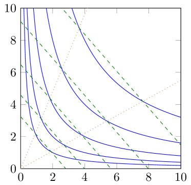
(a) $\xi\in\{2,4,8,16,32\}$, $(a_{1},a_{2})=(1,1)$, $(p,q)=(0.55,2.4)$

(b) $\xi\in\{1,2,3\}$, $(a_{1},a_{2})=(0.3,0.6)$, $(p,q)=(0.19,3.6)$

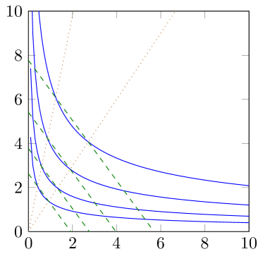
(c) $\xi\in\{8,2^{9},2^{15},2^{21}\}$, $(a_{1},a_{2})=(3.9,7.6)$, $(p,q)=(1.5,4.9)$

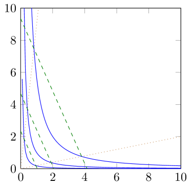
(d) $\xi\in\{0.5,1,2\}$, $(a_{1},a_{2})=(0.6,0.4)$, $(p,q)=(0.2,9)$

Figure 1. Solid lines are the level curves $\{{\boldsymbol{x}}\in\mathbb{R}_{+}^{2}:x_{1}^{a_{1}}x_{2}^{a_{2}}=\xi\}$; the dotted lines $x_{2}=px$ and $x_{2}=qx_{1}$ intersect each level curve in one point each. The dashed lines through the intersections of the level curves and the dotted lines are parallel to one another.

Let us illustrate the property on bivariate functions first. It is easy to show that for $n=2$ and $a_{1}=a_{2}=1$, $C_{\xi}\cap P_{ij}=\{\check{{\boldsymbol{x}}}\}$ and $C_{\xi}\cap Q_{ij}=\{\hat{{\boldsymbol{x}}}\}$ where

$$\check{{\boldsymbol{x}}}=\left(\sqrt{p\xi},\sqrt{\frac{1}{p}\xi}\right),\quad\hat{{\boldsymbol{x}}}=\left(\sqrt{q\xi},\sqrt{\frac{1}{q}\xi}\right).$$

The line through $\check{{\boldsymbol{x}}}$ and $\hat{{\boldsymbol{x}}}$ is given by the linear equation

$$\det\left(\left[\begin{array}[]{ccc}x_{1}&x_{2}&1\\ \sqrt{p\xi}&\sqrt{\frac{1}{p}\xi}&1\\ \sqrt{q\xi}&\sqrt{\frac{1}{q}\xi}&1\\ \end{array}\right]\right)=0,$$

and its slope $\frac{1/\sqrt{p}-1/\sqrt{q}}{\sqrt{p}-\sqrt{q}}=-(pq)^{-\frac{1}{2}}$ is independent of $\xi$. This also holds for general positive exponents $(a_{1},a_{2})\neq(1,1)$, in which case the coefficients of $x_{1}$ and $x_{2}$ are proportional to $\xi^{\frac{1}{\beta}}$ rather than $\sqrt{\xi}$. Figure 1 shows examples for different values of $a_{1}$, $a_{2}$, $p$, $q$, and $\xi$. We prove that this generalizes to $n\geq 2$.

Lemma 5.

Given ${\boldsymbol{a}}\in\mathbb{R}_{+}^{n}$, $i,j\in N$, $\xi\in\mathbb{R}$, $p,q\in\mathbb{R}_{+}$ with $i\neq j$ and $0<p<q$, there exist $d_{i}<0$ and $d_{j}>0$ such that for any $\check{\boldsymbol{x}}$ that satisfies $\check{x}_{j}=p\check{x}_{i}$ and $\prod_{i\in N}\check{x}_{i}^{a_{i}}=\xi$, there exists a unique solution $(\bar{s},\bar{\boldsymbol{x}})\in\mathbb{R}_{+}\times\mathbb{R}_{+}^{n}$ to the nonlinear system

(22) $$\bar{x}_{j}=q\bar{x}_{i}$$

(23) $$(\bar{x}_{i},\bar{x}_{j})=(\check{x}_{i}+\bar{s}d_{i},\check{x}_{j}+\bar{s}d_{j})$$

(24) $$\bar{x}_{k}=\check{x}_{k}\quad\forall k\notin\{i,j\}$$

(25) $$\textstyle\prod_{i\in N}\bar{x}_{i}^{a_{i}}=\xi.$$

Proof.

We prove that there exist $\eta_{1}$ and $\eta_{2}$ such that $(\bar{x}_{i},\bar{x}_{j})=(\eta_{i}\check{x}_{i},\eta_{j}\check{x}_{j})$. First, (25) requires $\prod_{k\in N}\bar{x}_{k}^{a_{k}}=\eta_{i}^{a_{i}}\eta_{j}^{a_{j}}\prod_{k\in N}\check{x}_{k}^{a_{k}}=\xi$, i.e., $\eta_{i}^{a_{i}}\eta_{j}^{a_{j}}=1$. Given that $\check{x}_{j}=p\check{x}_{i}$ and $\eta_{j}\check{x}_{j}=q\eta_{i}\check{x}_{i}$, solving both for $\frac{\check{x}_{i}}{\check{x}_{j}}$ yields $\frac{1}{p}=\frac{\eta_{j}}{q\eta_{i}}$, or

(26) $$\frac{\eta_{j}}{\eta_{i}}=\frac{q}{p}.$$

This yields $\eta_{i}=\left(\frac{q}{p}\right)^{-\frac{a_{j}}{a_{i}+a_{j}}}<1$ and $\eta_{j}=\eta_{i}\frac{q}{p}=\left(\frac{q}{p}\right)^{\frac{a_{i}}{a_{i}+a_{j}}}>1$.

In order to obtain $d_{i}$ and $d_{j}$, observe that

$$\begin{array}[]{lll}\check{x}_{i}+\bar{s}d_{i}=\eta_{i}\check{x}_{i}\\ \check{x}_{j}+\bar{s}d_{j}=\eta_{j}\check{x}_{j}.\\ \end{array}$$

Solving both for $\bar{s}$, we have $\frac{1}{d_{i}}\check{x}_{i}(\eta_{i}-1)=\frac{1}{d_{j}}\check{x}_{j}(\eta_{j}-1)$, and since $\frac{\check{x}_{i}}{\check{x}_{j}}=\frac{1}{p}$ we get

(27) $$\frac{d_{i}}{d_{j}}\frac{\eta_{j}-1}{\eta_{i}-1}=\frac{1}{p}.$$

For convenience, define fractions $\varphi_{i}=\frac{a_{i}}{a_{i}+a_{j}}$ and $\varphi_{j}=\frac{a_{j}}{a_{i}+a_{j}}$. Note that

$$\frac{\eta_{j}-1}{\eta_{i}-1}=\frac{q^{\varphi_{i}}-p^{\varphi_{i}}}{p^{\varphi_{i}}}\cdot\frac{p^{-\varphi_{j}}}{q^{-\varphi_{j}}-p^{-\varphi_{j}}}=\frac{q^{\varphi_{i}}-p^{\varphi_{i}}}{q^{-\varphi_{j}}-p^{-\varphi_{j}}}\cdot\frac{1}{p}.$$

Because $d_{i},d_{j}$ define a direction, rather than normalizing them (which would lead to complications in the next section) we determine $d_{i},d_{j}$ as denominator and numerator of the fraction above:

$$\begin{array}[]{llclc}d_{i}&=&q^{-\varphi_{j}}-p^{-\varphi_{j}}&=&q^{-a_{j}/(a_{i}+a_{j})}-p^{-a_{j}/(a_{i}+a_{j})}\\ d_{j}&=&q^{\varphi_{i}}-p^{\varphi_{i}}&=&q^{a_{i}/(a_{i}+a_{j})}-p^{a_{i}/(a_{i}+a_{j})}.\end{array}$$

Note that (i) $d_{i}<0<d_{j}$ (ii) both $d_{i}$ and $d_{j}$ only depend on $p$, $q$, $a_{i}$, and $a_{j}$, and not on $\check{x}_{i}$ or $\check{x}_{j}$; (iii) they are always defined. Hence, there exist unique $d_{i},d_{j}$ such that for any $\check{\boldsymbol{x}}$ such that $\check{x}_{j}=p\check{x}_{i}$, the parametric nonlinear system (22)–(25) admits the solution $(\bar{s},\bar{\boldsymbol{x}})\in\mathbb{R}_{+}\times\mathbb{R}_{+}^{n}$. Non-negativity of $\bar{\boldsymbol{x}}$, in particular of $\bar{x}_{i}$ and $\bar{x}_{j}$, follows from $0<\eta_{i}<1$ and $\eta_{j}>1$, while $\bar{s}\geq 0$ since $d_{i}<0$ and $\check{x}_{i}+\bar{s}d_{i}=\eta_{i}\check{x}_{i}\leq\check{x}_{i}$. ∎

Although $\bar{s}$ does depend on $\check{\boldsymbol{x}}$, the key fact is that direction $(d_{i},d_{j})$ defines a bijection from $P_{ij}$ to $Q_{ij}$ by joining pairs of points that have same value of the function $\prod_{i\in N}x_{i}^{a_{i}}$. This suggests that on a direction orthogonal to $(d_{i},d_{j})$, i.e., $(d_{j},-d_{i})$, we can define a lower-bounding function that matches the values on $P_{ij}$ and $Q_{ij}$ and that, for $n=2$, is the lower envelope of $f({\boldsymbol{x}})$.

Proposition 5.

The function $f^{\prime}_{\ell}({\boldsymbol{x}})=\lambda(d_{j}x_{i}-d_{i}x_{j})^{a_{i}+a_{j}}\prod_{k\in N\setminus\{i,j\}}x_{k}^{a_{k}}$, with $\lambda=p^{a_{j}}/\left(d_{j}-d_{i}p\right)^{a_{i}+a_{j}}$,

1. matches the value of $f({\boldsymbol{x}})$ for ${\boldsymbol{x}}\in P_{ij}\cup Q_{ij}$;

2. is a minorant of $f({\boldsymbol{x}})$ for ${\boldsymbol{x}}\in W_{ij}$;

3. is, for $n=2$ and $\beta=a_{1}+a_{2}\geq 1$, the lower envelope of $f({\boldsymbol{x}})$ in $W_{ij}$.

Proof.

a In order to prove $f^{\prime}_{\ell}({\boldsymbol{x}})=f({\boldsymbol{x}})\forall{\boldsymbol{x}}\in P_{ij}\cup Q_{ij}$, it suffices to prove that

$$\lambda(d_{j}x_{i}-d_{i}x_{j})^{a_{i}+a_{j}}=x_{i}^{a_{i}}x_{j}^{a_{j}}\,\forall x_{i},x_{j}:x_{j}=px_{i}\vee x_{j}=qx_{i}.$$

We prove this for ${\boldsymbol{x}}\in P_{ij}$ first. For $x_{j}=px_{i}$ we have

$$\begin{array}[]{rcl}\lambda(d_{j}x_{i}-d_{i}(px_{i}))^{a_{i}+a_{j}}&=&x_{i}^{a_{i}}(px_{i})^{a_{j}}\\ \lambda(d_{j}-pd_{i})^{a_{i}+a_{j}}x_{i}^{a_{i}+a_{j}}&=&p^{a_{j}}x_{i}^{a_{i}+a_{j}}\\ \lambda(d_{j}-pd_{i})^{a_{i}+a_{j}}&=&p^{a_{j}},\end{array}$$

which yields $\lambda=\frac{p^{a_{j}}}{(d_{j}-pd_{i})^{a_{i}+a_{j}}}$ in the statement. For $x_{j}=qx_{i}$ we obtain $\lambda^{\prime}=\frac{q^{a_{j}}}{(d_{j}-qd_{i})^{a_{i}+a_{j}}}$. To prove that $\lambda=\lambda^{\prime}$, observe that from (27) we obtain $d_{j}(\eta_{i}-1)=pd_{i}(\eta_{j}-1)$, which implies

$$d_{j}-pd_{i}=d_{j}\eta_{i}-pd_{i}\eta_{j}.$$

From (26) we obtain $p\eta_{j}=q\eta_{i}$, which means $d_{j}-pd_{i}=(d_{j}-qd_{i})\eta_{i}$. Also, $\eta_{i}^{a_{i}}\eta_{j}^{a_{j}}=1$ implies $\eta_{i}^{a_{i}}=\eta_{j}^{-a_{j}}$. Therefore,

$$\begin{array}[]{llll}\lambda^{\prime}&=&\frac{q^{a_{j}}}{(d_{j}-qd_{i})^{a_{i}+a_{j}}}\\ &=&\frac{q^{a_{j}}}{(d_{j}-pd_{i})^{a_{i}+a_{j}}\eta_{i}^{a_{i}+a_{j}}}\\ &=&\frac{q^{a_{j}}\eta_{j}^{a_{j}}}{(d_{j}-pd_{i})^{a_{i}+a_{j}}\eta_{i}^{a_{j}}},\\ \end{array}$$

but (26) implies $\frac{q^{a_{j}}\eta_{j}^{a_{j}}}{\eta_{i}^{a_{j}}}=p^{a_{j}}$, hence the two values of $\lambda$ match.

b First, $\tilde{\boldsymbol{x}}$ is a convex combination $\mu\check{\boldsymbol{x}}+(1-\mu)\hat{\boldsymbol{x}}$ of two points $\check{\boldsymbol{x}}\in P_{ij}$ and $\hat{\boldsymbol{x}}\in Q_{ij}$ such that $f^{\prime}_{\ell}(\check{\boldsymbol{x}})=f^{\prime}_{\ell}(\hat{\boldsymbol{x}})=f^{\prime}_{\ell}(\tilde{\boldsymbol{x}})$. We construct $\check{\boldsymbol{x}}$ and $\hat{\boldsymbol{x}}$ as follows: $\check{x}_{h}=\hat{x}_{h}=\tilde{x}_{h}$ for $i\neq h\neq j$; then we find $\check{x}_{i}$ and $\check{x}_{j}$ by solving the linear system $d_{j}\check{x}_{i}-d_{i}\check{x}_{j}=d_{j}\tilde{x}_{i}-d_{i}\tilde{x}_{j};\check{x}_{j}=p\check{x}_{i}$, and similar for $\hat{\boldsymbol{x}}$. It is easily proven that both systems admit a non-negative solution. Hence we have to prove that $f(\tilde{\boldsymbol{x}})\geq f(\check{\boldsymbol{x}})=f(\hat{\boldsymbol{x}})$. Note that $\tilde{x}_{i}=\mu\check{x}_{i}+(1-\mu)\eta_{i}\check{x}_{i}$ and similar for $\tilde{x}_{j}$, therefore

$$\begin{array}[]{lll}f(\tilde{\boldsymbol{x}})&=&\prod_{k\in N\setminus\{i,j\}}\tilde{x}_{k}^{a_{k}}\cdot\tilde{x}_{i}^{a_{i}}\tilde{x}_{j}^{a_{j}}\\ &=&\prod_{k\in N\setminus\{i,j\}}\check{x}_{k}^{a_{k}}\cdot\check{x}_{i}^{a_{i}}\check{x}_{j}^{a_{j}}\cdot(\mu+(1-\mu)\eta_{i})^{a_{i}}(\mu+(1-\mu)\eta_{j})^{a_{j}},\\ \end{array}$$

and we simply need to prove that $(\mu+(1-\mu)\eta_{i})^{a_{i}}(\mu+(1-\mu)\eta_{j})^{a_{j}}\geq 1$. By concavity of the logarithm,

$$\begin{array}[]{ll}&\log\left((\mu+(1-\mu)\eta_{i})^{a_{i}}(\mu+(1-\mu)\eta_{j})^{a_{j}}\right)\\ =&a_{i}\log(\mu+(1-\mu)\eta_{i})+a_{j}\log(\mu+(1-\mu)\eta_{j})\\ \geq&a_{i}(\mu\log(1)+(1-\mu)\log\eta_{i})+a_{j}(\mu\log(1)+(1-\mu)\log\eta_{j})\\ =&(1-\mu)(a_{i}\log\eta_{i}+a_{j}\log\eta_{j})\\ =&(1-\mu)\log(\eta_{i}^{a_{i}}\eta_{j}^{a_{j}})=0,\end{array}$$

which proves this part.

c For $n=2$, the function $f^{\prime}_{\ell}({\boldsymbol{x}})=\lambda(d_{j}x_{i}-d_{i}x_{j})^{\beta}$ is convex since $\beta\geq 1$. Building on a and b, suppose another convex function $g:\mathbb{R}^{2}\to\mathbb{R}$ exists such that $g({\boldsymbol{x}})\leq f({\boldsymbol{x}})$ for ${\boldsymbol{x}}\in W_{12}$ and there exists $\tilde{\boldsymbol{x}}$ such that $g(\tilde{\boldsymbol{x}})>f^{\prime}_{\ell}(\tilde{\boldsymbol{x}})$. Clearly $\tilde{\boldsymbol{x}}\notin(P_{ij}\cup Q_{ij})$ as otherwise a would imply $g(\tilde{\boldsymbol{x}})>f(\tilde{\boldsymbol{x}})$. Similar to the argument in b, consider then $\check{\boldsymbol{x}}\in P_{ij}$ and $\hat{\boldsymbol{x}}\in Q_{ij}$ such that $d_{2}\check{x}_{1}-d_{1}\check{x}_{2}=d_{2}\tilde{x}_{1}-d_{1}\tilde{x}_{2}=d_{2}\hat{x}_{1}-d_{1}\hat{x}_{2}$, i.e., the three points are aligned on a level curve of $f^{\prime}_{\ell}({\boldsymbol{x}})$. Obviously $\tilde{\boldsymbol{x}}$ is a convex combination (with weight denoted by $\mu$) of $\check{\boldsymbol{x}}$ and $\hat{\boldsymbol{x}}$ and $f(\check{\boldsymbol{x}})=f(\hat{\boldsymbol{x}})=f^{\prime}_{\ell}(\check{\boldsymbol{x}})=f^{\prime}_{\ell}(\hat{\boldsymbol{x}})=f^{\prime}_{\ell}(\tilde{\boldsymbol{x}})<g(\tilde{\boldsymbol{x}})$. This implies that $g(\tilde{\boldsymbol{x}})>\mu g(\check{\boldsymbol{x}})+(1-\mu)g(\hat{\boldsymbol{x}})$ and hence $g$ is not convex, a contradiction. ∎

Note that case c of the previous proposition is valid over the whole $W_{12}$; we are interested in the lower envelope over $X\cap W_{12}$, which will take an extra step. We first prove a similar result for $\beta\leq 1$.

Proposition 6.

For $\beta\leq 1$, the function

$$\textstyle f^{\prime\prime}_{\ell}({\boldsymbol{x}})=\zeta(d_{j}x_{i}-d_{i}x_{j})^{\frac{a_{i}+a_{j}}{\beta}}\left(\prod_{k\in N\setminus\{i,j\}}x_{k}^{a_{k}}\right)^{\frac{1}{\beta}}+z_{0},$$

with $\zeta=\lambda^{1/\beta}\frac{u-\ell}{u^{1/\beta}-\ell^{1/\beta}}$ and $z_{0}$ as defined in (12),

1. matches $f({\boldsymbol{x}})$ at $(P_{ij}\cup Q_{ij})\cap(C_{\ell}\cup C_{u})$;

2. is a minorant of $f$ in $X\cap W_{ij}$;

3. is the lower envelope of $f$ over $\textrm{conv}((P_{ij}\cup Q_{ij})\cap(C_{\ell}\cup C_{u}))$ for $n=2$.

Proof.

a From Proposition 5 (a-b), $\lambda(d_{j}x_{i}-d_{i}x_{j})^{a_{i}+a_{j}}\prod_{k\in N\setminus\{i,j\}}x_{k}^{a_{k}}$ is a minorant of $f$ within the same domain and matches $f$ in $P_{ij}\cup Q_{ij}$. Hence, for ${\boldsymbol{x}}\in P_{ij}\cup Q_{ij}$ such that $f({\boldsymbol{x}})=\ell$ we have $\lambda(d_{j}x_{i}-d_{i}x_{j})^{a_{i}+a_{j}}\prod_{k\in N\setminus\{i,j\}}x_{k}^{a_{k}}=\ell$, i.e., $(d_{j}x_{i}-d_{i}x_{j})^{\frac{a_{i}+a_{j}}{\beta}}\left(\prod_{k\in N\setminus\{i,j\}}x_{k}^{a_{k}}\right)^{\frac{1}{\beta}}=\left(\frac{\ell}{\lambda}\right)^{\frac{1}{\beta}}$, and similar for $u$. Therefore

$$\begin{array}[]{ll}\zeta\left(\frac{\ell}{\lambda}\right)^{\frac{1}{\beta}}+\zeta_{0}=\ell\\ \zeta\left(\frac{u}{\lambda}\right)^{\frac{1}{\beta}}+\zeta_{0}=u,\\ \end{array}$$

which is a linear system in $\zeta,\zeta_{0}$ with solutions

$$\begin{array}[]{l}\zeta=\frac{u-\ell}{\left(\frac{u}{\lambda}\right)^{\frac{1}{\beta}}-\left(\frac{\ell}{\lambda}\right)^{\frac{1}{\beta}}}=\lambda^{\frac{1}{\beta}}\frac{u-\ell}{u^{\frac{1}{\beta}}-\ell^{\frac{1}{\beta}}}=(\gamma\lambda)^{\frac{1}{\beta}}\\ \zeta_{0}=\ell-\zeta\left(\frac{\ell}{\lambda}\right)^{1/\beta}=\ell-\frac{(u-\ell)\ell^{1/\beta}}{u^{1/\beta}-\ell^{1/\beta}}=\frac{u^{1/\beta}\ell-\ell^{1/\beta}u}{u^{1/\beta}-\ell^{1/\beta}}=z_{0}.\end{array}$$

Therefore, $f^{\prime\prime}_{\ell}({\boldsymbol{x}})=f^{\prime}_{\ell}({\boldsymbol{x}})=f({\boldsymbol{x}})$ for ${\boldsymbol{x}}$ such that $x_{j}/x_{i}\in\{p,q\},f({\boldsymbol{x}})\in\{\ell,u\}$.

b By Lemma 3, if $\beta\leq 1$ then $f_{u}({\boldsymbol{x}})=z_{0}+\left(\gamma\prod_{k\in N}x_{k}^{a_{k}}\right)^{\frac{1}{\beta}}$ is a minorant of $f({\boldsymbol{x}})$ for $f({\boldsymbol{x}})\in[\ell,u]$. Therefore it suffices to prove that $f^{\prime\prime}_{\ell}({\boldsymbol{x}})\leq f_{u}({\boldsymbol{x}})$ in $X\cap W_{ij}$.

$$\begin{array}[]{lrlr}&z_{0}+\zeta(d_{j}x_{i}-d_{i}x_{j})^{\frac{a_{i}+a_{j}}{\beta}}\left(\prod_{k\in N\setminus\{i,j\}}x_{k}^{a_{k}}\right)^{\frac{1}{\beta}}&\leq&z_{0}+\left(\gamma\prod_{k\in N}x_{k}^{a_{k}}\right)^{\frac{1}{\beta}}\\ \Leftrightarrow&(\gamma\lambda)^{\frac{1}{\beta}}(d_{j}x_{i}-d_{i}x_{j})^{\frac{a_{i}+a_{j}}{\beta}}\left(\prod_{k\in N\setminus\{i,j\}}x_{k}^{a_{k}}\right)^{\frac{1}{\beta}}&\leq&\left(\gamma\prod_{k\in N}x_{k}^{a_{k}}\right)^{\frac{1}{\beta}}\\ \Leftrightarrow&\lambda^{\frac{1}{\beta}}(d_{j}x_{i}-d_{i}x_{j})^{\frac{a_{i}+a_{j}}{\beta}}\phantom{\left(\prod_{k\in N\setminus\{i,j\}}x_{k}^{a_{k}}\right)^{\frac{1}{\beta}}}&\leq&\left(x_{i}^{a_{i}}x_{j}^{a_{j}}\right)^{\frac{1}{\beta}}.\end{array}$$

The last inequality is equivalent to $\lambda(d_{j}x_{i}-d_{i}x_{j})^{a_{i}+a_{j}}\leq x_{i}^{a_{i}}x_{j}^{a_{j}}$, which holds in $X\cap W_{ij}$ for Proposition 5. Although it is applied here to the two-variable monomial $x_{i}^{a_{i}}x_{j}^{a_{j}}$ rather than $f({\boldsymbol{x}})$, the relationship still holds because $d_{i},d_{j}$ only depend on $p,q,a_{i},a_{j}$, and $\lambda$ depends on $d_{i},d_{j},p,q,a_{i},a_{j}$.

c For $n=2$, $f^{\prime\prime}_{\ell}({\boldsymbol{x}})$ reduces to the linear function $\zeta(d_{2}x_{1}-d_{1}x_{2})+z_{0}$. By a and b, $f^{\prime\prime}_{\ell}$ matches the concave function $f({\boldsymbol{x}})$ at all four points of the set $T=(P_{ij}\cup Q_{ij})\cap(C_{\ell}\cup C_{u})$. For linearity of $f^{\prime\prime}_{\ell}$, any function $g$ defined on $\textrm{conv}(T)$ such that $g(\tilde{\boldsymbol{x}})>f^{\prime\prime}_{\ell}(\tilde{\boldsymbol{x}})$ for some $\tilde{\boldsymbol{x}}\in\textrm{conv}(T)$ is concave w.r.t. two or more elements of $T$, and hence cannot be the (convex) lower envelope of $f$ over $\textrm{conv}(T)$. ∎

Lemma 6.

For $n=2$, the convex hull of $X\cap W_{12}$ is

$$\begin{array}[]{ll}Y=\!\!&\{{\boldsymbol{x}}\in\mathbb{R}^{2}_{+}:\\ &\phantom{\{}px_{1}\leq x_{2}\leq qx_{1},\\ &\phantom{\{}x_{1}^{a_{1}}x_{2}^{a_{2}}\geq\ell,\\ &\phantom{\{}d_{2}x_{1}-d_{1}x_{2}\leq(u/\lambda)^{\frac{1}{\beta}}\}.\end{array}$$

Proof.

$\lambda(d_{2}x_{1}-d_{1}x_{2})^{\beta}\leq f({\boldsymbol{x}})$ and $f({\boldsymbol{x}})\leq u$ imply $d_{2}x_{1}-d_{1}x_{2}\leq(u/\lambda)^{\frac{1}{\beta}}$ and consequently $X\cap W_{12}\subseteq Y$. By convexity of $Y$ we also have $\textrm{conv}(X\cap W_{12})\subseteq Y$. In order to prove $\textrm{conv}(X\cap W_{12})\supseteq Y$, consider $\tilde{\boldsymbol{x}}\in Y$. If $\tilde{\boldsymbol{x}}\in X\cap W_{12}$, the result holds. Otherwise $f(\tilde{\boldsymbol{x}})>u\geq\lambda(d_{2}\tilde{x}_{1}-d_{1}\tilde{x}_{2})^{\beta}$. Consider two vectors $\check{\boldsymbol{x}}\in P_{12}$ and $\hat{\boldsymbol{x}}\in Q_{12}$ such that $d_{2}\check{x}_{1}-d_{1}\check{x}_{2}=d_{2}\hat{x}_{1}-d_{1}\hat{x}_{2}=d_{2}\tilde{x}_{1}-d_{1}\tilde{x}_{2}$. Such points satisfy the two systems

$$\left\{\begin{array}[]{l}d_{2}\check{x}_{1}-d_{1}\check{x}_{2}=d_{2}\tilde{x}_{1}-d_{1}\tilde{x}_{2}\\ p\check{x}_{1}-\check{x}_{2}=0\end{array}\right.\qquad\left\{\begin{array}[]{l}d_{2}\hat{x}_{1}-d_{1}\hat{x}_{2}=d_{2}\tilde{x}_{1}-d_{1}\tilde{x}_{2}\\ q\hat{x}_{1}-\hat{x}_{2}=0,\end{array}\right.$$

both of which always yield a solution as $d_{2},p,q>0$ and $d_{1}<0$. Because $\check{\boldsymbol{x}}\in P_{12}$, $\hat{\boldsymbol{x}}\in Q_{12}$, and $f^{\prime}_{\ell}({\boldsymbol{x}})=\lambda(d_{2}x_{1}-d_{1}x_{2})^{\beta}=\lambda(d_{2}\tilde{x}_{1}-d_{1}\tilde{x}_{2})^{\beta}\leq u$ for both $\check{\boldsymbol{x}}$ and $\hat{\boldsymbol{x}}$, these belong to $X\cap W_{12}$ and $\tilde{\boldsymbol{x}}$ is their convex combination since $\frac{\check{x}_{2}}{\check{x}_{1}}=p\leq\frac{\tilde{x}_{2}}{\tilde{x}_{1}}\leq q=\frac{\hat{x}_{2}}{\hat{x}_{1}}$, proving that $\tilde{\boldsymbol{x}}\in\textrm{conv}(X\cap W_{12})$. ∎

The last condition defining $Y$, i.e., $d_{2}x_{1}-d_{1}x_{2}\leq(u/\lambda)^{\frac{1}{\beta}}$, is equivalent to setting an upper bound of $u$ on the lower-bounding function $f^{\prime}_{\ell}({\boldsymbol{x}})$ for $\beta\geq 1$, as it is equivalent to $\lambda(d_{2}x_{1}-d_{1}x_{2})^{\beta}\leq u$. It is also equivalent to setting an upper bound of $u$ on the lower-bounding function $f^{\prime\prime}_{\ell}({\boldsymbol{x}})$ for the case $\beta\leq 1$: $f^{\prime\prime}_{\ell}({\boldsymbol{x}})=\zeta(d_{2}x_{1}-d_{1}x_{2})+z_{0}\leq u$ if $d_{2}x_{1}-d_{1}x_{2}\leq\frac{u-z_{0}}{\zeta}$, but

$$\frac{u-z_{0}}{\zeta}=\frac{u-z_{0}}{\lambda^{\frac{1}{\beta}}\frac{u-\ell}{u^{\frac{1}{\beta}}-\ell^{\frac{1}{\beta}}}}=\frac{u^{\frac{1}{\beta}}-\ell^{\frac{1}{\beta}}}{\lambda^{\frac{1}{\beta}}(u-\ell)}\left(u-\frac{u^{\frac{1}{\beta}}\ell-\ell^{\frac{1}{\beta}}u}{u^{\frac{1}{\beta}}-\ell^{\frac{1}{\beta}}}\right)=\frac{u^{\frac{1}{\beta}}}{\lambda^{\frac{1}{\beta}}}.$$

Because $f$ is defined over $\mathbb{R}_{+}^{n}$, Lemma 6 defines the projection onto the ${\boldsymbol{x}}$-space of the lower and upper envelopes of $f$ over $X\cap W_{12}$ and consequently the projection of $\textrm{conv}(F(W_{12}))$. The argument used in the above proof is worth underlining and will be used below: a vector $\tilde{\boldsymbol{x}}\in Y$ such that $f(\tilde{\boldsymbol{x}})>u\geq f^{\prime}_{\ell}(\tilde{\boldsymbol{x}})$ is a member of $\textrm{conv}(X\cap W_{12})$.

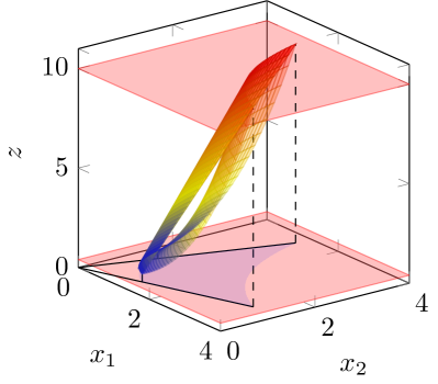
(a) The upper envelope $f^{\prime}_{u}(x_{1},x_{2})=z_{0}+(\gamma x_{1}^{a_{1}}x_{2}^{a_{2}})^{\frac{1}{\beta}}$.

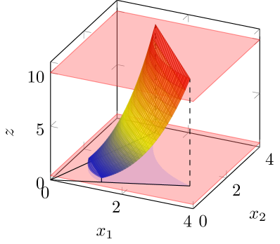
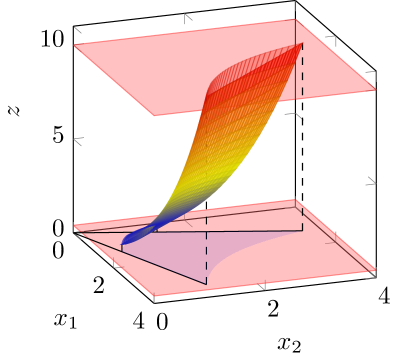
(b) The lower envelope $f^{\prime}_{\ell}(x_{1},x_{2})=\lambda(d_{2}x_{1}-d_{1}x_{2})^{\beta}$.

Figure 2. Upper envelope $f^{\prime}_{u}({\boldsymbol{x}})$ (top) and lower envelope $f^{\prime}_{\ell}({\boldsymbol{x}})$ of function $f({\boldsymbol{x}})=x_{1}^{a_{1}}x_{2}^{a_{2}}$ for $\beta\geq 1$, both shown under different angles. The domain $\{(x_{1},x_{2})\in\mathbb{R}_{+}^{2}:px_{1}\leq x_{2}\leq qx_{1},f({\boldsymbol{x}})\in[\ell,u]\}$ is the shaded area on the $x_{1},x_{2}$ plane. The parameters are as follows: $(p,q)=(0.35,3)$, $(\ell,u)=(0.4,10)$, $(a_{1},a_{2})=(1.7,1.5)$.

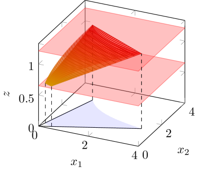
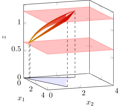
Figure 3. Lower envelope $f^{\prime\prime}_{\ell}({\boldsymbol{x}})$ of function $f({\boldsymbol{x}})=x_{1}^{a_{1}}x_{2}^{a_{2}}$ shown under different angles. The domain $\{(x_{1},x_{2})\in\mathbb{R}_{+}^{2}:px_{1}\leq x_{2}\leq qx_{1},f({\boldsymbol{x}})\in[\ell,u]\}$ is the shaded area on the $x,y$ plane. The parameters are as follows: $(p,q)=(0.4,3.3)$, $(\ell,u)=(0.65,1.21)$, $(a_{1},a_{2})=(0.1,0.2)$.

We are now ready to provide the upper envelope of $f$ over $X\cap W_{ij}$ for $n=2$, which was left uncovered from the previous section. Figures 2 and 3 show upper and lower envelopes for sample values of the parameters. The proof is, up to Case 1 included, similar to the proof of Proposition 3 for $n>2$.

Theorem 1.

For $n=2$, the upper envelope $E_{U}(f,X\cap W_{12})$ is

$$\begin{array}[]{rcl}&H=\!\!&\{({\boldsymbol{x}},z)\in Y\times\mathbb{R}:\\ &&z\leq f_{u}({\boldsymbol{x}})\\ &&z\leq u\},\end{array}$$

where $f_{u}({\boldsymbol{x}})=f^{\prime}_{u}({\boldsymbol{x}})=z_{0}+\left(\gamma x_{1}^{a_{1}}x_{2}^{a_{2}}\right)^{\frac{1}{\beta}}$ if $\beta\geq 1$ and $f_{u}({\boldsymbol{x}})=f({\boldsymbol{x}})$ otherwise.

Proof.

Any $({\boldsymbol{x}},z)\in\textrm{hyp}(f,X\cap W_{ij})$ satisfies ${\boldsymbol{x}}\in Y$ for Lemma 6 and $z\leq u$ as ${\boldsymbol{x}}\in X$. Also, $({\boldsymbol{x}},z)$ satisfies $z\leq f_{u}({\boldsymbol{x}})$: by construction for $\beta\leq 1$, and by Lemma 3 for $\beta\geq 1$. Hence $\textrm{hyp}(f,X\cap W_{ij})\subseteq H$. Because $H$ is convex, $E_{U}(f,X\cap W_{ij})\subseteq H$. We now prove that $H\subseteq E_{U}(f,X\cap W_{ij})$. Consider $(\tilde{\boldsymbol{x}},\tilde{z})\in H$. Two cases arise: either $\tilde{x}_{1}^{a_{1}}\tilde{x}_{2}^{a_{2}}\leq u$ or $\tilde{x}_{1}^{a_{1}}\tilde{x}_{2}^{a_{2}}>u$.

Case 1: $\tilde{x}_{1}^{a_{1}}\tilde{x}_{2}^{a_{2}}\leq u$.

If $\beta\leq 1$ or $\tilde{z}\leq\tilde{x}_{1}^{a_{1}}\tilde{x}_{2}^{a_{2}}$, then obviously $(\tilde{\boldsymbol{x}},\tilde{z})\in\textrm{hyp}(f,X\cap W_{12})$ and the result holds. Otherwise, see Case 1, proof of Proposition 3.

Case 2: $\tilde{x}_{1}^{a_{1}}\tilde{x}_{2}^{a_{2}}>u$.

There exist $\check{\boldsymbol{x}}=s^{\prime}\tilde{\boldsymbol{x}}$ such that $f(\check{\boldsymbol{x}})=f_{u}(\check{\boldsymbol{x}})=u$ (again, by construction for $\beta\leq 1$ and by Lemma 3 for $\beta\geq 1$) and $\hat{\boldsymbol{x}}=s^{\prime\prime}\tilde{\boldsymbol{x}}$ such that $\lambda(d_{2}\hat{x}_{1}-d_{1}\hat{x}_{2})^{\beta}=f^{\prime}_{\ell}(\hat{\boldsymbol{x}})=u\leq f(\hat{\boldsymbol{x}})$. Because $\tilde{\boldsymbol{x}}$ satisfies $\lambda(d_{2}\tilde{x}_{1}-d_{1}\tilde{x}_{2})^{\beta}\leq u$ and $f^{\prime}_{\ell}$ is monotone increasing along the direction $\{s\tilde{\boldsymbol{x}}:s\geq 0\}$, $s^{\prime\prime}$ is unique and $s^{\prime\prime}\geq 1$. Similarly, $s^{\prime}$ is unique and $s^{\prime}<1$. Then $\tilde{\boldsymbol{x}}$ is a convex combination of $\check{\boldsymbol{x}}$ and $\hat{\boldsymbol{x}}$.

Whereas $(\check{\boldsymbol{x}},z)\in\textrm{hyp}(f,X\cap W_{ij})$ for $z\leq u$, $\hat{\boldsymbol{x}}$ is in turn a convex combination of two points in $X\cap W_{ij}$: $\check{{\boldsymbol{x}}}$ and $\hat{{\boldsymbol{x}}}$ such that $f(\check{{\boldsymbol{x}}})=f(\hat{{\boldsymbol{x}}})=u$, $x^{p}_{2}=px^{p}_{1}$, and $x^{q}_{2}=qx^{q}_{1}$. Properties of $f^{\prime}_{\ell}$ show that $f^{\prime}_{\ell}(\check{{\boldsymbol{x}}})=f^{\prime}_{\ell}(\hat{{\boldsymbol{x}}})=f^{\prime}_{\ell}(\hat{\boldsymbol{x}})=u$, which implies $\check{{\boldsymbol{x}}},\hat{{\boldsymbol{x}}},\hat{\boldsymbol{x}}$ lie on the same level line of $f^{\prime}_{\ell}$ and $d_{2}x^{p}_{1}-d_{1}x^{p}_{2}=d_{2}x^{q}_{1}-d_{1}x^{q}_{2}=d_{2}\check{x}_{1}-d_{1}\check{x}_{2}=\left(\frac{u}{\lambda}\right)^{\frac{1}{\beta}}$. Taking into account $z$, the above implies implies $(\tilde{\boldsymbol{x}},u)$ is a convex combination of $(\check{\boldsymbol{x}},u)$, $(\check{{\boldsymbol{x}}},u)$, and $(\hat{{\boldsymbol{x}}},u)$, all elements of $X\cap W_{12}$. But then $(\check{\boldsymbol{x}},\tilde{z})$, $(\check{{\boldsymbol{x}}},\tilde{z})$, and $(\hat{{\boldsymbol{x}}},\tilde{z})$ all belong to $\textrm{hyp}(f,X\cap W_{ij})$ by definition of hypograph, and because $\tilde{z}\leq u$, $(\tilde{\boldsymbol{x}},\tilde{z})$ is their convex combination hence $(\tilde{\boldsymbol{x}},\tilde{z})\in E_{U}(f,X\cap W_{ij})$. ∎

Theorem 2.

For $n=2$, the lower envelope $E_{L}(f,X\cap W_{12})$ is

$$\begin{array}[]{rcl}&H=\!\!&\{({\boldsymbol{x}},z)\in Y\times\mathbb{R}:\\ &&z\geq f_{\ell}({\boldsymbol{x}}),\\ &&z\geq\ell\},\end{array}$$

where $f_{\ell}({\boldsymbol{x}})=f^{\prime}_{\ell}({\boldsymbol{x}})$ if $\beta\geq 1$ and $f_{\ell}({\boldsymbol{x}})=f^{\prime\prime}_{\ell}({\boldsymbol{x}})$ if $\beta\leq 1$.

Proof.

Any $(\tilde{\boldsymbol{x}},\tilde{z})\in\textrm{epi}(f,X\cap W_{12})$ satisfies ${\boldsymbol{x}}\in Y$ and $z\geq\ell$ by definition. It also satisfies $z\geq f^{\prime}_{\ell}({\boldsymbol{x}})$ by Proposition 5 and $z\geq f^{\prime\prime}_{\ell}({\boldsymbol{x}})$ by Proposition 6. Hence $\textrm{epi}(f,X\cap W_{12})\subseteq H$. By convexity of $H$ we conclude $E_{L}(f,X\cap W_{12})\subseteq H$. We prove now $H\subseteq E_{L}(f,X\cap W_{12})$.

Consider $(\tilde{\boldsymbol{x}},\tilde{z})\in H$. If $\tilde{\boldsymbol{x}}\in\textrm{conv}((C_{\ell}\cup C_{u})\cap(P_{12}\cup Q_{12}))$, then for $\beta\leq 1$ the vector $(\tilde{\boldsymbol{x}},f^{\prime\prime}_{\ell}({\boldsymbol{x}}))$ is a convex combination of the four vectors $(\dot{\boldsymbol{x}},f^{\prime\prime}_{\ell}(\dot{\boldsymbol{x}}))=(\dot{\boldsymbol{x}},f(\dot{\boldsymbol{x}}))$ for $\dot{\boldsymbol{x}}\in(C_{\ell}\cup C_{u})\cap(P_{12}\cup Q_{12})$, given that $f^{\prime\prime}_{\ell}$ is linear (see Proposition 6). For $\beta\geq 1$, $f^{\prime}_{\ell}$ matches $f$ within $P_{12}\cup Q_{12}$ (see Proposition 5), hence there exist $\hat{\boldsymbol{x}},\check{\boldsymbol{x}}$ such that $(\tilde{\boldsymbol{x}},f^{\prime}_{\ell}({\boldsymbol{x}}))$ is a convex combination of $(\hat{\boldsymbol{x}},f^{\prime}_{\ell}(\hat{\boldsymbol{x}}))$ and $(\check{\boldsymbol{x}},f^{\prime}_{\ell}(\check{\boldsymbol{x}}))$, both in $\textrm{epi}(f,X\cap W_{12})$. In both cases, $z\geq f_{\ell}({\boldsymbol{x}})$ and therefore $(\tilde{\boldsymbol{x}},\tilde{z})\in E_{L}(f,X\cap W_{12})$.

If $\tilde{\boldsymbol{x}}\in Y\setminus\textrm{conv}((C_{\ell}\cup C_{u})\cap(P_{12}\cup Q_{12}))$, then $f({\boldsymbol{x}})\geq\ell\geq f_{\ell}({\boldsymbol{x}})$. A similar argument to the above leads to three points $\check{\boldsymbol{x}}\in C_{\ell}\cap P_{12}$, $\hat{\boldsymbol{x}}\in C_{\ell}\cap Q_{12}$ (these two sets contain a single vector each), and $\dot{\boldsymbol{x}}$, such that $f(\dot{\boldsymbol{x}})=f(\check{\boldsymbol{x}})=f(\hat{\boldsymbol{x}})=\ell$ and that form $(\tilde{\boldsymbol{x}},\ell)$ as their convex combination, where $\tilde{z}\geq\ell$, yielding $(\tilde{\boldsymbol{x}},\tilde{z})\in E_{L}(f,X\cap W_{12})$. This concludes the proof; note that $Y\setminus\textrm{int}(\textrm{conv}((C_{\ell}\cup C_{u})\cap(P_{12}\cup Q_{12})))$ is the convex hull of $C_{\ell}\cap W_{12}$. ∎

Given a function $f$ and its lower and upper envelopes $f^{\prime\prime}_{\ell}$ and $f^{\prime\prime}_{u}$ over a set $\mathcal{D}$, the convex hull of $\{({\boldsymbol{x}},z)\in\mathbb{R}^{n+1}:z=f({\boldsymbol{x}})\}$ is given by the intersection of lower and upper envelope [27]. The convex hull of $X\cap W_{ij}$ for $n=2$ is hence the intersection of the upper and lower envelope described above.

Unlike the convex hull for $n=2$, the one for $n>2$ has one key feature: its projection onto the ${\boldsymbol{x}}$ variables is unbounded. For this reason the extra linear inequality $d_{2}x_{1}-d_{1}x_{2}\leq\left(\frac{u}{\lambda}\right)^{\frac{1}{\beta}}$ is only valid for $n=2$.

Corollary 1.

The convex hull of $F(W_{12})$ for $n=2$ and $\beta\geq 1$ is

$$\begin{array}[]{rl}\textrm{conv}(F(W_{12}))=\!&\{({\boldsymbol{x}},z)\in Y\times\mathbb{R}:\\ &\max\{\ell,\lambda(d_{2}x_{1}-d_{1}x_{2})^{\beta}\}\leq z\leq\min\{u,z_{0}+(\gamma x_{1}^{a_{1}}x_{2}^{a_{2}})^{\frac{1}{\beta}}\}\}.\end{array}$$

The convex hull of $F(W_{12})$ for $n=2$ and $\beta\leq 1$ is

$$\begin{array}[]{rl}\textrm{conv}(F(W_{12}))=\!&\{({\boldsymbol{x}},z)\in Y\times\mathbb{R}:\\ &\max\{\ell,\zeta(d_{2}x_{1}-d_{1}x_{2})+z_{0}\}\leq z\leq\min\{u,x_{1}^{a_{1}}x_{2}^{a_{2}}\}\}.\end{array}$$

For $\beta\geq 1$, the upper envelope $f^{\prime}_{u}$ matches $f$ only on the level sets of $f$, i.e., $C_{\ell}\cup C_{u}=\{{\boldsymbol{x}}\in\mathbb{R}_{+}^{2}:f(x)\in\{\ell,u\}\}$, and the lower envelope $f^{\prime}_{\ell}$ matches $f$ on the set $P\cup Q=\{{\boldsymbol{x}}\in\mathbb{R}_{+}^{2}:x_{2}=px_{1}\vee x_{2}=qx_{1}\}$. For $\beta\leq 1$, the upper envelope $f^{\prime\prime}_{u}$ matches $f$ in $(P\cup Q)\cup(C_{\ell}\cup C_{u})$, while the lower envelope $f^{\prime\prime}_{\ell}$ matches $f$ in four points: those of the set $(P_{12}\cup Q_{12})\cap(C_{\ell}\cup C_{u})$.

Table 1 summarizes the results from this and the previous two sections. The lower envelope for $W_{ij}$ is an open problem for $n>2$.

	$\beta\geq 1$	$\beta\leq 1$
	$n\geq 2$
$\textrm{conv}(F(\mathbb{R}_{+}^{n}))$	$\begin{array}[]{c}{\boldsymbol{x}}\in\mathbb{R}_{+}^{n}\\ (z-z_{0})^{\beta}\leq\gamma\prod_{k\in N}x_{k}^{a_{k}}\\ z\in[\ell,u]\end{array}$	$\begin{array}[]{c}{\boldsymbol{x}}\in\mathbb{R}_{+}^{n}\\ z\leq\prod_{k\in N}x_{k}^{a_{k}}\\ z\in[\ell,u]\end{array}$
$E_{U}(f,X\cap W_{ij})$	$\begin{array}[]{c}{\boldsymbol{x}}\in\mathbb{R}_{+}^{n}\\ (z-z_{0})^{\beta}\leq\gamma\prod_{k\in N}x_{k}^{a_{k}}\\ z\leq u\\ px_{i}\leq x_{j}\leq qx_{i}\\ \prod_{k\in N}x_{k}^{a_{k}}\geq\ell\end{array}$	$\begin{array}[]{c}{\boldsymbol{x}}\in\mathbb{R}_{+}^{n}\\ z\leq\prod_{k\in N}x_{k}^{a_{k}}\\ z\leq u\\ px_{i}\leq x_{j}\leq qx_{i}\\ \prod_{k\in N}x_{k}^{a_{k}}\geq\ell\end{array}$
	$n=2$
$E_{L}(f,X\cap W_{ij})$	$\begin{array}[]{c}px_{1}\leq x_{2}\leq qx_{1}\\ x_{1}^{a_{1}}x_{2}^{a_{2}}\geq\ell\\ d_{2}x_{1}-d_{1}x_{2}\leq(u/\lambda)^{\frac{1}{\beta}}\\ z\geq\lambda(d_{2}x_{1}-d_{1}x_{2})^{\beta}\\ z\geq\ell\\ \end{array}$	$\begin{array}[]{c}px_{1}\leq x_{2}\leq qx_{1}\\ x_{1}^{a_{1}}x_{2}^{a_{2}}\geq\ell\\ d_{2}x_{1}-d_{1}x_{2}\leq(u/\lambda)^{\frac{1}{\beta}}\\ z\geq\zeta(d_{2}x_{1}-d_{1}x_{2})+z_{0}\\ z\geq\ell\\ \end{array}$
$E_{U}(f,X\cap W_{ij})$	$\begin{array}[]{c}px_{1}\leq x_{2}\leq qx_{1}\\ x_{1}^{a_{1}}x_{2}^{a_{2}}\geq\ell\\ d_{2}x_{1}-d_{1}x_{2}\leq(u/\lambda)^{\frac{1}{\beta}}\\ (z-z_{0})^{\beta}\leq\gamma x_{1}^{a_{1}}x_{2}^{a_{2}}\\ z\leq u\\ \end{array}$	$\begin{array}[]{c}px_{1}\leq x_{2}\leq qx_{1}\\ x_{1}^{a_{1}}x_{2}^{a_{2}}\geq\ell\\ d_{2}x_{1}-d_{1}x_{2}\leq(u/\lambda)^{\frac{1}{\beta}}\\ z\leq x_{1}^{a_{1}}x_{2}^{a_{2}}\\ z\leq u\\ \end{array}$

Table 1. Summary of results on lower and upper envelopes of $f$ over $X$ and over $X\cap W_{ij}$.

5. Volume of the convex hull

Computing the volume of the convex hull of $f({\boldsymbol{x}})$ within $X\cap W_{12}$ finds a practical application in choosing branching rules in a MINLO solver. Branching decisions affect the efficiency of any BB algorithm in a strong and often unpredictable way. Even for the most standard branching decision $(x_{k}\leq b^{\prime})\vee(x_{k}\geq b^{\prime\prime})$, there is no supporting evidence of any single best branching policy for choosing the branching variable $x_{k}$ [1, 7] or the branching point $b^{\prime},b^{\prime\prime}$ [5].

The volume of the convex hull of nonlinear operators has been considered for bi- and tri-linear terms $x_{i}x_{j}$ and $x_{i}x_{j}x_{k}$ [13, 24, 26, 14], as a measure for quality of relaxations and for evaluating branching rules [25]–see also Anstreicher et al. [3].

Mixed Integer Linear Optimization (MILO) algorithms only concern themselves with choosing a branching variable at each node, but this is not the case for MINLO problems. Once a branching variable $x_{k}$ is chosen, balanced branching attempts to create balanced BB subtrees by selecting a branching point such that the convex hulls of the feasible set of each of the two resulting subproblems have equal volume, in the hope of creating two balanced BB subtrees [22, 5]. An alternative branching criterion is that the resulting total volume of the convex hulls of the two subproblems is minimum. Rather than computing the volume of said convex hulls of the new feasible regions, it is more practical to compute it for the operators containing the branched-on variable.

We assume $n=2$ from now on. The feasible region for a two-variable monomial term $z=x_{1}^{a_{1}}x_{2}^{a_{2}}$ considered here is defined by bounds $z\in[\ell,u]$ on the monomial itself and by the $p,q$ parameters defining the homogeneous inequalities $px_{1}\leq x_{2}\leq qx_{1}$ delimiting $x_{1}$ and $x_{2}$. Branching on $z$ and on $x_{1}/x_{2}$ allows for maintaining tight relaxations by using the convex envelopes described in this article. Therefore one can consider two branching rules: given $r\in(p,q)$, either branch using $(px_{1}\leq x_{2}\leq rx_{1})\vee(rx_{1}\leq x_{2}\leq qx_{1})$ or using $(z\leq\nu)\vee(z\geq\nu)$.

Two questions arise: once the monomial term has been chosen for branching, do we branch on $z$ or on $\frac{x_{2}}{x_{1}}$? Also, what is the branching point $\nu$ or $r$ that minimizes the total volume in the two subproblems or, alternatively, finds the most balanced pair of subproblems?

(a) $(p,q)=(0.35,3)$, $(a_{1},a_{2})=(1.7,1.5)$, $(\ell,u)=(0.4,10)$, $z=4.4$

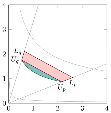
(b) $(p,q)=(0.4,3.3)$, $(a_{1},a_{2})=(0.1,0.2)$, $(\ell,u)=(0.65,1.21)$, $z=1.05$

Figure 4. Cross-section (two shades) of the convex envelope of $f({\boldsymbol{x}})=x_{1}^{a_{1}}x_{2}^{a_{2}}$ for $z\in[\ell,u]$ in the region $W_{12}=\{(x_{1},x_{2})\in\mathbb{R}_{+}^{2}:px_{1}\leq x_{2}\leq qx_{1}\}$, for $\beta\geq 1$ (left) and $\beta\leq 1$. For $\beta\geq 1$, the level curve of $f({\boldsymbol{x}})$ is the dashed arc between $L_{p}$ and $L_{q}$. The arc between $U_{p}$ and $U_{q}$ is the level curve of the upper envelope $\hat{f}({\boldsymbol{x}})=z_{0}+\left(\gamma x_{1}^{a_{1}}x_{2}^{a_{2}}\right)^{\frac{1}{\beta}}$ (left) and the level set for $f({\boldsymbol{x}})$ (right). Finally, the segment $L_{p}L_{q}$ is the level curve of the lower envelope $f^{\prime}_{\ell}({\boldsymbol{x}})=\lambda(d_{2}x_{1}-d_{1}x_{2})^{\beta}=z$ (left) and $f^{\prime\prime}_{\ell}({\boldsymbol{x}})=\zeta(d_{2}x_{1}-d_{1}x_{2})+z_{0}=z$ (right), for the given value of $z$.

Given an initial set defined by $p,q,\ell,u,a_{1},a_{2}$, the volume of the convex envelope denoted as $V(p,q,\ell,u)$, a branching rule on $x_{j}/x_{i}$ using $r$ as a ratio results in a total volume of $V_{r}=V(p,r,\ell,u)+V(r,q,\ell,u)$, while a branching rule on $z$ with branching value $\nu$ results in a total volume of $V_{b}(\nu)=V(p,q,\ell,\nu)+V(p,q,\nu,u)$. If the minimum total volume is sought, one must select between two minimizers: $r\in\textrm{argmin}\{V_{r}(r):r\in[p+\epsilon,q-\epsilon]\}$ and $\nu\in\textrm{argmin}\{V_{b}(\nu):\nu\in[\ell+\epsilon,u-\epsilon]\}$. Here $\epsilon$ is used to obtain tighter bound interval on $\nu$ and $r$, which ensures that the feasible regions of both new subproblems are strict subsets of the subproblem being branched on. Balanced branching requires instead $V(p,r,\ell,u)=V(r,q,\ell,u)$ and $V(p,q,\ell,\nu)=V(p,q,\nu,u)$ respectively. Therefore, an analytical form of the volume of the convex hull described in Corollary 1 would be useful.

Both envelopes of $f$ over $X\cap W_{12}$, i.e., $\max\{\ell,f_{\ell}({\boldsymbol{x}})\}$ (lower) and $\min\{u,f_{u}({\boldsymbol{x}})\}$ (upper), are non-smooth as $f_{\ell}$ and $f_{u}$ have non-null gradient in all of $W_{12}$ (except for $f^{\prime}_{\ell}$ at ${\boldsymbol{x}}=0$). The domain $\mathcal{D}$ makes it additionally awkward to consider each envelope separately.

Consider any $z$ in the range $[\ell,u]$ of $z$. The volume differential $dV$ at $z$ is the product of $dz$ and the area of the cross-section of the convex envelope at $z$. Integrating the volume differential yields the volume of the convex hull. The main advantage of this method is that the structure of the cross-section only depends on $z$ and the original parameters of the problem.

Figure 4 illustrates the cross-section as a shaded region, which we subdivide into two areas (indicated by different shades) for ease of computation. The shape of the cross-section is roughly the same for $\beta\geq 1$ and $\beta\leq 1$. The segment $L_{p}L_{q}$ is the level curve of the lower envelope $f^{\prime}_{\ell}({\boldsymbol{x}})$ (for $\beta\geq 1$) and $f^{\prime\prime}_{\ell}({\boldsymbol{x}})$ (for $\beta\leq 1$), while the arc between $U_{p}$ and $U_{q}$ is the level curve of the upper envelope $f_{u}({\boldsymbol{x}})$. Together with the lines $x_{2}=px_{1}$ and $x_{2}=qx_{1}$ defining $P_{12}$ and $Q_{12}$, these delimit the cross-section. The dashed arc between $L_{p}$ and $L_{q}$ is the level curve of $f({\boldsymbol{x}})$ at $z$ for $\beta\geq 1$ (see Figure 4a) and is only shown for completeness; it will not be used in our derivation.

As proven in Section 4, the extremes $U_{p},U_{q}$ of the arc also form a segment that is parallel to $L_{p}L_{q}$. The area of the cross-section is hence the sum of two areas: that of the lightly-shaded trapezoid with vertices $L_{p},L_{q},U_{q},U_{p}$ and the dark-shaded area between the arc and the segment both delimited by $U_{p},U_{q}$.

Trapezoid.

The area of the trapezoid $L_{p}L_{q}U_{q}U_{p}$ is $\frac{1}{2}\left(\Delta_{\textsc{u}}+\Delta_{\textsc{l}}\right)\delta$, where $\Delta_{\textsc{u}}$ and $\Delta_{\textsc{l}}$ are the lengths of $U_{p}U_{q}$ and $L_{p}L_{q}$, respectively, and $\delta$ is the distance between these two parallel segments. We need $x_{1},x_{2}$ coordinates of all four points: $L_{p}=(x_{1}^{\textsc{l}p},x_{2}^{\textsc{l}p})$, $L_{q}=(x_{1}^{\textsc{l}q},x_{2}^{\textsc{l}q})$, $U_{p}=(x_{1}^{\textsc{u}p},x_{2}^{\textsc{u}p})$, $U_{q}=(x_{1}^{\textsc{u}q},x_{2}^{\textsc{u}q})$. Then $\Delta_{\textsc{l}}$ and $\Delta_{\textsc{u}}$ are $\|{\boldsymbol{x}}^{\textsc{l}p}-{\boldsymbol{x}}^{\textsc{l}q}\|_{2}$ and $\|{\boldsymbol{x}}^{\textsc{u}p}-{\boldsymbol{x}}^{\textsc{u}q}\|_{2}$ respectively.

$$\begin{array}[]{rl}\Delta_{\textsc{l}}&=\left((x_{1}^{\textsc{l}p}-x_{1}^{\textsc{l}q})^{2}+(px_{1}^{\textsc{l}p}-qx_{1}^{\textsc{l}q})^{2})\right)^{\frac{1}{2}}\\ &=\left((1+p^{2})(x_{1}^{\textsc{l}p})^{2}+(1+q^{2})(x_{1}^{\textsc{l}q})^{2}-2(1+pq)x_{1}^{\textsc{l}p}x_{1}^{\textsc{l}q}\right)^{\frac{1}{2}}\\ &=x_{1}^{\textsc{l}p}\left(1+p^{2}+\eta_{1}^{2}(1+q^{2})-2\eta_{1}(1+pq)\right)^{\frac{1}{2}}\\ &=x_{1}^{\textsc{l}p}\left(1+p^{2}+\eta_{1}^{2}+\eta_{1}^{2}q^{2}-2\eta_{1}-2\eta_{1}pq\right)^{\frac{1}{2}}\\ &=x_{1}^{\textsc{l}p}\left((1-\eta_{1})^{2}+p^{2}+\eta_{2}^{2}p^{2}-2\eta_{2}p^{2}\right)^{\frac{1}{2}}\\ &=x_{1}^{\textsc{l}p}\left((1-\eta_{1})^{2}+p^{2}(1-\eta_{2})^{2}\right)^{\frac{1}{2}}.\end{array}$$

Define $\tau=\sqrt{(1-\eta_{1})^{2}+p^{2}(1-\eta_{2})^{2}}$. Then $\Delta_{\textsc{l}}=\tau x_{1}^{\textsc{l}p}$ and $\Delta_{\textsc{u}}=\tau x_{1}^{\textsc{u}p}$.

In order to compute $\delta$, consider the equations of the line through ${\boldsymbol{x}}^{\textsc{u}p}$ and ${\boldsymbol{x}}^{\textsc{u}q}$ and the one through ${\boldsymbol{x}}^{\textsc{l}p}$ and ${\boldsymbol{x}}^{\textsc{l}q}$. They have the same slope,

$$\sigma=\frac{d_{2}}{d_{1}}=p\frac{\eta_{2}-1}{\eta_{1}-1}<0.$$

Then the two equations are $x_{2}=\sigma x_{1}+(x_{2}^{\textsc{u}p}-\sigma x_{1}^{\textsc{u}p})$ and $x_{2}=\sigma x_{1}+(x_{2}^{\textsc{l}p}-\sigma x_{1}^{\textsc{l}p})$. The former equation is used below to compute the area of the remaining part of the cross-section. The distance between two lines with equal slope $x_{2}=\sigma x_{1}+r^{\prime}$ and $x_{2}=\sigma x_{1}+r^{\prime\prime}$ is $\frac{\lvert r^{\prime\prime}-r^{\prime}\rvert}{\sqrt{1+\sigma^{2}}}$, therefore

$$\textstyle\delta=\frac{\lvert(x_{2}^{\textsc{u}p}-\sigma x_{1}^{\textsc{u}p})-(x_{2}^{\textsc{l}p}-\sigma x_{1}^{\textsc{l}p})\rvert}{\sqrt{1+\sigma^{2}}}=\frac{\lvert(p-\sigma)x_{1}^{\textsc{u}p}-(p-\sigma)x_{1}^{\textsc{l}p}\rvert}{\sqrt{1+\sigma^{2}}}=\frac{p-\sigma}{\sqrt{1+\sigma^{2}}}(x_{1}^{\textsc{l}p}-x_{1}^{\textsc{u}p}).$$

Hence the area of the trapezoid is

$$A_{1}(z)=\frac{1}{2}\delta(\Delta_{\textsc{l}}+\Delta_{\textsc{u}})=\frac{\tau(p-\sigma)}{2\sqrt{1+\sigma^{2}}}((x_{1}^{\textsc{l}p})^{2}-(x_{1}^{\textsc{u}p})^{2}).$$

Note that $\sqrt{1+\sigma^{2}}=\sqrt{1+p^{2}\left(\frac{\eta_{2}-1}{\eta_{1}-1}\right)^{2}}=\frac{1}{1-\eta_{1}}\sqrt{(\eta_{1}-1)^{2}+p^{2}(\eta_{2}-1)^{2}}$ and that $p-\sigma=p-p\frac{\eta_{2}-1}{\eta_{1}-1}=p\frac{\eta_{2}-\eta_{1}}{\eta_{1}-1}$, therefore

$$\frac{\tau(p-\sigma)}{2\sqrt{1+\sigma^{2}}}=\frac{p}{2}(\eta_{2}-\eta_{1}).$$

In the remainder of this section, the calculation for the cross-section area is divided for the two cases $\beta\geq 1$ and $\beta\leq 1$.

Case 1: $\beta\geq 1$

The coordinates $(x_{1}^{\textsc{l}p},x_{2}^{\textsc{l}p})$ of $L_{p}$ satisfy $\lambda(d_{2}x_{1}^{\textsc{l}p}-d_{1}x_{2}^{\textsc{l}p})^{\beta}=x_{1}^{a_{1}}x_{2}^{a_{2}}=z$ (because $f^{\prime}_{\ell}$ matches $f$ on $P\cup Q$), whereas those of $U_{p}$ satisfy $z_{0}+\left(\gamma(x_{1}^{\textsc{u}p})^{a_{1}}(x_{2}^{\textsc{u}p})^{a_{2}}\right)^{\frac{1}{\beta}}=z$; both satisfy $x_{2}=px_{1}$. Therefore

$$\begin{array}[]{rlll}(x^{\textsc{l}p}_{1})^{a_{1}}(px^{\textsc{l}p}_{1})^{a_{2}}=z&\Leftrightarrow&x_{1}^{\textsc{l}p}=(p^{-a_{2}}z)^{\frac{1}{\beta}}\\ z_{0}+\left(\gamma p^{a_{2}}(x_{1}^{\textsc{u}p})^{\beta}\right)^{\frac{1}{\beta}}=z&\Leftrightarrow&x_{1}^{\textsc{u}p}=\frac{z-z_{0}}{(\gamma p^{a_{2}})^{\frac{1}{\beta}}},\\ \end{array}$$

and similarly for other points we obtain

(28) $$\begin{array}[]{lllll}x_{1}^{\textsc{l}p}=(p^{-a_{2}}z)^{\frac{1}{\beta}},&x_{2}^{\textsc{l}p}=px_{1}^{\textsc{l}p},&&x_{1}^{\textsc{u}p}=\frac{z-z_{0}}{(\gamma p^{a_{2}})^{\frac{1}{\beta}}},&x_{2}^{\textsc{u}p}=px_{2}^{\textsc{u}p},\\ x_{1}^{\textsc{l}q}=(q^{-a_{2}}z)^{\frac{1}{\beta}},&x_{2}^{\textsc{l}q}=qx_{1}^{\textsc{l}q},&&x_{1}^{\textsc{u}q}=\frac{z-z_{0}}{(\gamma q^{a_{2}})^{\frac{1}{\beta}}},&x_{2}^{\textsc{u}q}=qx_{2}^{\textsc{u}q}.\\ \end{array}$$

The area of the trapezoid is hence $A_{1}(z)=\frac{1}{2}p(\eta_{2}-\eta_{1})\left(z^{\frac{2}{\beta}}-(z-z_{0})^{2}/\gamma^{\frac{2}{\beta}}\right)$.

The area defined by arc and segment between $U_{p}$ and $U_{q}$ is equal to the integral of the difference between two functions: the linear function through $U_{p}$ and $U_{q}$, $x_{2}=\sigma x_{1}+(x_{2}^{\textsc{u}p}-\sigma x_{1}^{\textsc{u}p})$, and the function $x_{2}=\left((\frac{z-z_{0}}{\gamma})^{\beta}x_{1}^{-a_{1}}\right)^{\frac{1}{a_{2}}}$ which arises from solving $z_{0}+\gamma(x_{1}^{a_{1}}x_{2}^{a_{2}})^{\frac{1}{\beta}}=z$ for $x_{2}$.

The difference is $\sigma x_{1}+(p-\sigma)x_{1}^{\textsc{u}p}-(\frac{z-z_{0}}{\gamma})^{\frac{\beta}{a_{2}}}x_{1}^{-\frac{a_{1}}{a_{2}}}$, whose primitive is

$$\left\{\begin{array}[]{ll}\frac{1}{2}\sigma x_{1}^{2}+(p-\sigma)x_{1}^{\textsc{u}p}x_{1}-\frac{a_{2}}{a_{2}-a_{1}}(\frac{z-z_{0}}{\gamma})^{\frac{\beta}{a_{2}}}x_{1}^{\frac{a_{2}-a_{1}}{a_{2}}}&\textrm{ if }a_{1}\neq a_{2}\\ \frac{1}{2}\sigma x_{1}^{2}+(p-\sigma)x_{1}^{\textsc{u}p}x_{1}-(\frac{z-z_{0}}{\gamma})^{\frac{\beta}{a_{2}}}\log x_{1}&\textrm{ otherwise},\\ \end{array}\right.$$

which yields, for $a_{1}\neq a_{2}$,

$$\begin{array}[]{rcl}A_{2}(z)=&\frac{1}{2}\sigma((x_{1}^{\textsc{u}p})^{2}-(x_{1}^{\textsc{u}q})^{2})+(p-\sigma)(x_{1}^{\textsc{u}p}-x_{1}^{\textsc{u}q})-\\ &\frac{a_{2}}{a_{2}-a_{1}}(\frac{z-z_{0}}{\gamma})^{\frac{\beta}{a_{2}}}((x_{1}^{\textsc{u}p})^{\frac{a_{2}-a_{1}}{a_{2}}}-(x_{1}^{\textsc{u}q})^{\frac{a_{2}-a_{1}}{a_{2}}}),\end{array}$$

and $A_{2}(z)=\frac{1}{2}\sigma((x_{1}^{\textsc{u}p})^{2}-(x_{1}^{\textsc{u}q})^{2})+(p-\sigma)(x_{1}^{\textsc{u}p}-x_{1}^{\textsc{u}q})-(\frac{z-z_{0}}{\gamma})^{\frac{\beta}{a_{2}}}(\log x_{1}^{\textsc{u}p}-\log x_{1}^{\textsc{u}q})$ otherwise.

The total area of the cross-section is then a polynomial function with terms $z^{\frac{2}{\beta}}$, $(z-z_{0})^{2}$, and $(z-z_{0})^{\frac{\beta}{a_{2}}}$. For simplicity we write it as $A(z)=b_{1}z^{\frac{2}{\beta}}+b_{2}(z-z_{0})^{2}+b_{3}(z-z_{0})^{\frac{\beta}{a_{2}}}$ for opportune values of $b_{1},b_{2},b_{3}$ which depend on $a_{1},a_{2},p,q,\ell,u$. Therefore the volume of the convex hull for $n=2$ is $\textrm{Vol}(\textrm{conv}(X\cap W_{12}))=\int_{\ell}^{u}A(z)dz$, i.e.,

$$\begin{array}[]{ll}&\left[b_{1}\frac{\beta}{\beta+2}z^{1+\frac{2}{\beta}}+\frac{1}{3}b_{2}(z-z_{0})^{3}+\frac{a_{2}}{a_{2}+\beta}b_{3}(z-z_{0})^{1+\frac{\beta}{a_{2}}}\right]_{\ell}^{u}\\ =&b_{1}\frac{\beta}{\beta+2}(u^{1+\frac{2}{\beta}}-\ell^{1+\frac{2}{\beta}})+\frac{1}{3}b_{2}\left((u-z_{0})^{3}-(\ell-z_{0})^{3}\right)+\\ &\frac{a_{2}}{a_{2}+\beta}b_{3}\left((u-z_{0})^{1+\frac{\beta}{a_{2}}}-(\ell-z_{0})^{1+\frac{\beta}{a_{2}}}\right),\end{array}$$

where $b_{3}$ is defined differently depending on whether $a_{1}=a_{2}$ or not.

Case 2: $\beta\leq 1$

For $L_{p}$ one must solve the system $x_{2}^{lp}=px_{1}^{lp},z=\zeta(d_{2}x_{1}^{lp}-d_{1}x_{2}^{lp})+z_{0}$ for $x_{1}^{lp}$, which yields $x_{1}^{lp}=\frac{z-z_{0}}{(d_{2}-d_{1}p)\zeta}=\frac{(z-z_{0})\big{(}u^{\frac{1}{\beta}}-\ell^{\frac{1}{\beta}}\big{)}}{(u-\ell)q^{\frac{a_{2}}{\beta}}}$. For $U_{p}$ and $U_{q}$, note that $f$ constitutes the upper envelope, hence $(x_{1}^{\textsc{u}p})^{a_{1}}(x_{2}^{\textsc{u}p})^{a_{2}}=z$ and $x_{2}^{\textsc{u}p}=px_{1}^{\textsc{u}p}$ yields $x_{1}^{\textsc{u}p}=z^{\frac{1}{\beta}}p^{-a_{2}}$. Then the area of the trapezoid specializes to

$$A_{1}(z)=\frac{p}{2}(\eta_{2}-\eta_{1})\left(\left(\frac{(z-z_{0})\big{(}u^{\frac{1}{\beta}}-\ell^{\frac{1}{\beta}}\big{)}}{(u-\ell)q^{\frac{a_{2}}{\beta}}}\right)^{2}-(z^{\frac{1}{\beta}}p^{-a_{2}})^{2}\right).$$

Finally, the curve delimiting $X\cap W_{12}$ from below has equation $x_{2}=z^{\frac{1}{a_{2}}}x_{1}^{-\frac{a_{1}}{a_{2}}}$, while the line between ${\boldsymbol{x}}^{\textsc{u}q}$ and ${\boldsymbol{x}}^{\textsc{u}p}$ is $x_{2}=x_{2}^{\textsc{u}p}+\sigma(x_{1}-x_{1}^{\textsc{u}p})=\sigma x_{1}+x_{1}^{\textsc{u}p}(p-\sigma)=\sigma x_{1}+(p-\sigma)z^{\frac{1}{\beta}}p^{-a_{2}}$. The area of $\textrm{conv}(C_{\ell}\cap W_{12})$ is then the integral, between $x_{1}^{\textsc{u}q}$ and $x_{1}^{\textsc{u}p}$, of the function $\sigma x_{1}+(p-\sigma)z^{\frac{1}{\beta}}p^{-a_{2}}-z^{\frac{1}{a_{2}}}x_{1}^{-\frac{a_{1}}{a_{2}}}$, whose primitive is similar, in structure, to that for the case $\beta\geq 1$, and thus we omit it here. The volume of the convex hull for $\beta\leq 1$ is therefore an integral of a polynomial in $z$ with the same exponents as for $\beta\geq 1$, but with different coefficients due to different coordinates of $L_{p},L_{q},U_{p},U_{q}$.

6. Concluding remarks and open questions

We considered the monomial $f({\boldsymbol{x}})=\prod_{k\in N}x_{k}^{a_{k}}$, with positive exponents, for ${\boldsymbol{x}}\in\mathbb{R}_{+}^{n}$. We proved that its upper envelope, for general $n\geq 2$, is a conic function when the domain of $f$ restrict its value between $\ell\geq 0$ and $u$. The result holds even when two variables $x_{i},x_{j}$, apart from being non-negative, are also constrained to form a linear cone $px_{i}\leq x_{j}\leq qx_{i}$ pointed at the origin.

For $n=2$ and when maintaining the linear cone $px_{1}\leq x_{2}\leq qx_{1}$, we also find the lower envelope of $f({\boldsymbol{x}})$ and thus are able to describe the convex hull of $F(W_{12})$ and its volume.

A seemingly easy extension that we have not considered here is the case with $n=2,a_{1},a_{2}<0$, which makes $f$ convex and perhaps yields a convex hull similar to that of the case $\beta\leq 1$.

As discussed in Section 1, these results are applicable to either problems whose model has constraints such as $px_{i}\leq x_{j}\leq qx_{i}$ or algorithms that enforce such constraints as cutting planes or branching operations. If such wedge constraints are not a natural way to describe a problem or an algorithm, the obvious tradeoff is between two approaches for MINLO:

• the classic approach, where variables have initial lower and upper bounds and branching rules are of the form $x_{k}\leq b\vee x_{k}\geq b$, but the convex hull of $\{(x_{1},x_{2})\in\mathbb{R}_{+}^{2}:x_{1}^{a_{1}}x_{2}^{a_{2}}\in[\ell,u],x_{1}\in[\ell_{1},u_{1}],x_{2}\in[\ell_{2},u_{2}]\}$ is not known and therefore a decomposition like the one described in Section 1 is needed;

• an approach where the conic constraint $px_{1}\leq x_{2}\leq qx_{1}$ is enforced and the convex hull is known.

Such tradeoff can make one or the other relaxation tighter. Computational tests are needed to assess the quality of the convex hull above, especially because the partitioning of $\mathbb{R}_{+}^{2}$ through linear inequalities is not as standard as variable bounds.

References

Achterberg et al. [2005]
T. Achterberg, T. Koch, and A. Martin.
Branching rules revisited.
OR Letters, 33(1):42–54, 2005.
Al-Khayyal and Falk [1983]
F. A. Al-Khayyal and J. E. Falk.
Jointly constrained biconvex programming.
Mathematics of Operations Research, 8:273–286,
1983.
Anstreicher et al. [2021]
K. M. Anstreicher, S. Burer, and K. Park.
Convex hull representations for bounded products of variables.
Journal of Global Optimization, 80:757–778, 2021.
Belotti et al. [2009]
P. Belotti, J. Lee, L. Liberti, F. Margot, and A. Wächter.
Branching and bounds tightening techniques for non-convex MINLP.
Optimization Methods & Software, 24(4-5):597–634, 2009.
Belotti et al. [2010]
P. Belotti, A. J. Miller, and M. Namazifar.
Valid inequalities and convex hulls for multilinear functions.
Electronic Notes in Discrete Mathematics, 36:805–812, 2010.
ISSN 1571-0653.
doi: 10.1016/j.endm.2010.05.102.
ISCO 2010 - International Symposium on Combinatorial Optimization.
Bénichou et al. [1971]
M. Bénichou, J. M. Gauthier, P. Girodet, G. Hentges, G. Ribière, and
O. Vincent.
Experiments in mixed-integer linear programming.
Mathematical Programming, 1:76–94, 1971.
Bestuzheva et al. [2021]
K. Bestuzheva, M. Besançon, W.-K. Chen, A. Chmiela, T. Donkiewicz, J. van
Doornmalen, L. Eifler, O. Gaul, G. Gamrath, A. Gleixner, et al.
The SCIP optimization suite 8.0.
arXiv preprint arXiv:2112.08872, 2021.
Boyd et al. [2007]
S. Boyd, S.-J. Kim, L. Vandenberghe, and A. Hassibi.
A tutorial on geometric programming.
Optimization and Engineering, 8(1):67–127, 2007.
Ecker [1980]
J. G. Ecker.
Geometric programming: methods, computations and applications.
SIAM review, 22(3):338–362, 1980.
Horst and Tuy [1993]
R. Horst and H. Tuy.
Global Optimization.
Springer-Verlag, New York, 1993.
Lee et al. [2018]
J. Lee, D. Skipper, and E. Speakman.
Algorithmic and modeling insights via volumetric comparison of
polyhedral relaxations.
Mathematical Programming, 170(1):121–140,
2018.
Lee et al. [2019]
J. Lee, D. Skipper, and E. Speakman.
Gaining or losing perspective.
In World Congress on Global Optimization, pages 387–397.
Springer, 2019.
Lu et al. [2010]
H.-C. Lu, H.-L. Li, C. E. Gounaris, and C. A. Floudas.
Convex relaxation for solving posynomial programs.
Journal of Global Optimization, 46(1):147–154, 2010.
McCormick [1976]
G. P. McCormick.
Computability of global solutions to factorable nonconvex programs:
Part I — Convex underestimating problems.
Mathematical Programming, 10:146–175, 1976.
Meyer and Floudas [2004]
C. A. Meyer and C. A. Floudas.
Trilinear monomials with mixed sign domains: Facets of the convex and
concave envelopes.
Journal of Global Optimization, 29(2), 2004.
Misener and Floudas [2014]
R. Misener and C. A. Floudas.
Antigone: algorithms for continuous/integer global optimization of
nonlinear equations.
Journal of Global Optimization, 59(2-3):503–526, 2014.
Neumeier [1990]
A. Neumeier.
Interval methods for systems of equations.
Cambridge Univ. Press, Cambridge, 1990.
Nguyen et al. [2018]
T. T. Nguyen, J.-P. P. Richard, and M. Tawarmalani.
Deriving convex hulls through lifting and projection.
Mathematical Programming, 169(2):377–415,
2018.
Rikun [1997]
A. D. Rikun.
A convex envelope formula for multilinear functions.
Journal of Global Optimization, 10:425–437, 1997.
Sahinidis [1996]
N. Sahinidis.
Baron: a general purpose global optimization software package.
Journal of Global Optimization, 8:201–205, 1996.
Smith and Pantelides [1999]
E. M. B. Smith and C. C. Pantelides.
A symbolic reformulation/spatial branch-and-bound algorithm for the
global optimisation of nonconvex MINLPs.
Computers & Chem. Eng., 23:457–478, 1999.
Speakman and Lee [2017]
E. Speakman and J. Lee.
Quantifying double McCormick.
Mathematics of Operations Research, 42(4):1230–1253, 2017.
Speakman and Lee [2018]
E. Speakman and J. Lee.
On branching-point selection for trilinear monomials in spatial
branch-and-bound: the hull relaxation.
Journal of Global Optimization, 72(2):129–153, 2018.
Speakman et al. [2017]
E. Speakman, H. Yu, and J. Lee.
Experimental validation of volume-based comparison for
double-McCormick relaxations.
In International Conference on AI and OR Techniques in
Constraint Programming for Combinatorial Optimization Problems, pages
229–243. Springer, 2017.
Tawarmalani and Richard [2013]
M. Tawarmalani and J.-P. P. Richard.
Decomposition techniques in convexification of inequalities.
Technical report, Technical report, 2013.
Tawarmalani and Sahinidis [2002]
M. Tawarmalani and N. V. Sahinidis.
Convexification and Global Optimization in Continuous and
Mixed-Integer Nonlinear Programming: Theory, Algorithms, Software, and
Applications.
Kluwer Academic Publishers, Boston MA, 2002.
Tsai and Lin [2011]
J.-F. Tsai and M.-H. Lin.
An efficient global approach for posynomial geometric programming
problems.
INFORMS Journal on Computing, 23(3):483–492, 2011.