Evolutionary Dynamic Optimization Laboratory: A MATLAB Optimization Platform for Education and Experimentation in Dynamic Environments

Abstract.

Abstract— Many real-world optimization problems possess dynamic characteristics. Evolutionary dynamic optimization algorithms (EDOAs) aim to tackle the challenges associated with dynamic optimization problems. Looking at the existing works, the results reported for a given EDOA can sometimes be considerably different. This issue occurs because the source codes of many EDOAs, which are usually very complex algorithms, have not been made publicly available. Indeed, the complexity of components and mechanisms used in many EDOAs makes their re-implementation error-prone. In this paper, to assist researchers in performing experiments and comparing their algorithms against several EDOAs, we develop an open-source MATLAB platform for EDOAs, called Evolutionary Dynamic Optimization LABoratory (EDOLAB). This platform also contains an education module that can be used for educational purposes. In the education module, the user can observe a) a 2-dimensional problem space and how its morphology changes after each environmental change, b) the behaviors of individuals over time, and c) how the EDOA reacts to environmental changes and tries to track the moving optimum. In addition to being useful for research and education purposes, EDOLAB can also be used by practitioners to solve their real-world problems. The current version of EDOLAB includes 25 EDOAs and three fully-parametric benchmark generators. The MATLAB source code for EDOLAB is publicly available and can be accessed from [https://github.com/EDOLAB-platform/EDOLAB-MATLAB].

1. Introduction

Many real-world optimization problems are dynamic (Nguyen, 2011), meaning that the characteristics of the search spaces of these problems change over time (Yazdani et al., 2021b; Raquel and Yao, 2013). Environmental changes in dynamic optimization problems (DOPs) generate uncertainties that cannot be relaxed/removed and need to be taken into account by the optimization algorithm (Jin and Branke, 2005). To solve many DOPs, it is important that the optimization algorithm can efficiently locate an optimal solution and also track it after environmental changes. This process is known as tracking the moving optimum (TMO) (Nguyen et al., 2012).

Evolutionary algorithms and swarm intelligence methods are popular and effective optimization tools that were originally designed for solving static optimization problems. However, directly using these optimization tools for TMO in DOPs is ineffective because they do not take the environmental changes into account. Environmental changes in DOPs cause several challenges for these methods, including a) outdated stored fitness values, b) local and global diversity loss, and c) limited number of fitness values that can be evaluated between two consecutive environmental changes (i.e., in each environment) (Yazdani et al., 2020a). To cope with optimization in dynamic environments and address the challenges of performing TMO in DOPs, evolutionary algorithms and swarm intelligence methods are usually combined with some other components to form evolutionary dynamic optimization algorithms (EDOAs). These components include local diversity control, global diversity control, explicit archive, change detection, change reaction, population clustering, population management, exclusion, convergence detection, and computational resource allocation (Yazdani et al., 2021b). As a result, they are usually complex algorithms.

The complexity of EDOAs, the state-of-the-art ones in particular, makes them hard to re-implement. This issue sometimes results in reporting significantly different results for a given EDOA (Yazdani et al., 2021c) because re-implementing them is error-prone. The lack of publicly available source codes for many EDOAs has caused a significant challenge for researchers in reproducing the results for experimentation and comparisons. Aside from the EDOAs, the process of calculating the performance indicators and also the dynamic benchmark generators are complex as well. Looking at some of the few available source codes, we realized that the performance indicators, such as offline error (Branke and Schmeck, 2003), are calculated in a wrong way. Moreover, in some source codes, some parameters of the popular moving peaks benchmark (MPB) (Branke, 1999), such as the random number generators and initial values of peaks’ parameters, are set in ways that resulted in unfair comparisons. Furthermore, there is no considerable platform available in the field for evaluating the performance of EDOAs and identifying both their weaknesses and strengths in solving DOP instances with various morphological and dynamical characteristics (Herring et al., 2022).

Considering the aforementioned issues, there is a lack of a comprehensive software platform in the field. To address the urgent demand for such software, we developed an open-source MATLAB platform for EDOAs called Evolutionary Dynamic Optimization LABoratory (EDOLAB). The current version of EDOLAB focuses on single-objective unconstrained continuous DOPs. However, the designed EDOAs for this class of DOPs are shown to be easily extendable to tackle other important classes of DOPs, such as robust optimization over time (ROOT) (Yazdani et al., 2023a, 2022), constrained DOPs (Nguyen and Yao, 2012; Bu et al., 2016), and large-scale DOPs (Luo et al., 2017; Yazdani et al., 2019). Furthermore, although the structures of EDOAs designed for single-objective DOPs are different from those designed for finding Pareto optimal solutions (POS) in each environment in multi-objective DOPs (Jiang et al., 2022), they are still effective for tackling many multi-objective DOPs. Indeed, in many multi-objective DOPs, there is one solution deployed in each environment, which is chosen by a decision maker based on preferences. Thus, finding POS for each environment and picking a solution for deployment may not be the best option for many problems, e.g., the ones with high change frequencies. For example, given a real-world multi-objective DOP whose environment changes every few seconds, it is challenging for a user to pick a solution from POS for each environment. To solve such multi-objective DOPs, the problem can be transformed into a single-objective DOP by combining all objectives according to the preferences (Marler and Arora, 2010; Kaddani et al., 2017). Consequently, in the resulting single-objective problem, a single-objective EDOA can be used, which focuses on finding an optimal solution for deployment in each environment according to the preferences.

In the following, we describe the major contributions and features of EDOLAB:

Comprehensive library

The current release of EDOLAB includes 25 EDOAs, which are listed in Table 1, with various characteristics, including different structures, optimizers, population clustering and sub-population management methods, diversity control components, and computational resource allocation methods. EDOLAB also contains three dynamic benchmark generators that are MPB (Branke, 1999), free peaks (FPs) (Li et al., 2018), and Generalized MPB (GMPB) (Yazdani et al., 2020b, 2021a). These benchmark generators are fully configurable by parameters, and they can generate countless numbers of dynamic problem instances with various morphological and dynamical characteristics. In addition, to measure the efficiency of EDOAs in solving DOPs and facilitate comparisons, the two most commonly used performance indicators –offline error (Branke and Schmeck, 2003) and the average error before environmental changes (Trojanowski and Michalewicz, 1999)– are used in EDOLAB.

Easy to use

The programming language used for developing EDOLAB is MATLAB. The large collection of high-level mathematical functions to operate on arrays and matrices along with various random number generators make MATLAB suitable for implementing EDOAs and dynamic benchmarks. Thanks to the features of MATLAB, the source codes of EDOLAB, EDOAs and benchmarks in particular, are easy to understand, trace, and modify. In addition, by choosing informative names for parameters, distinguishing different components, and adding enlightening comments, we endeavor to further improve the understandability and clarity of the source codes. EDOLAB also benefits from a graphical user interface (GUI) that makes it easy to use, especially for beginners. Using the GUI, the user can easily choose an EDOA, configure a problem instance, and run the experiment.

Multi-purpose usability

EDOLAB can be used either with or without the GUI for empirical studies. Thanks to the rich library of EDOLAB, researchers can easily investigate and compare the performance of different EDOAs with various structures and components on problem instances with different dynamical and morphological characteristics. In addition, researchers who develop new EDOAs can evaluate their algorithms using the source codes provided in EDOLAB. In particular, our platform provides three benchmark generators capable of creating countless problem instances with different characteristics and levels of difficulty, as well as various comparison EDOAs, performance indicators, and plots useful in evaluating new algorithms and writing scientific reports and articles. Moreover, EDOLAB includes a module for educational purposes, whose main target audience is beginners. This module shows the chosen 2-dimensional problem space (i.e., environment) and how its morphology changes after each environmental change. The user can also observe the similarity factors between successive environments to understand the reasons behind the importance of knowledge transfer from the previous to the current environment in EDOAs (Nguyen et al., 2012). Moreover, by showing the individuals’ relocation over time, their behavior can be observed by the user. Another important observation is the relocation of individuals at the beginning of each environment, which helps the user to understand how each EDOA reacts to the environmental changes and tries to track the moving optimum.

Extensibility

EDOLAB is easy to extend, and researchers are able to expand EDOLAB’s library by adding other EDOAs, benchmark problems, and performance indicators. In addition, using EDOLAB’s open-source codes, researchers can modify EDOA frameworks, embed their own components in them, and investigate their effectiveness. For example, if a researcher designs a new exclusion, change reaction, or convergence detection component, she/he can replace the part of the code that belongs to the old component with that of the newly designed one and examine its impact on the overall performance of an EDOA. Furthermore, researchers can expand the EDOAs to solve other classes of DOPs by adding specific components necessary for solving them, e.g., adding constraint handling components for solving constrained DOPs (Nguyen and Yao, 2012) or decision makers for changing or keeping deployed solutions in ROOT (Yazdani et al., 2017; Yazdani et al., 2018a). The flexibility and extensibility of EDOLAB also make the practitioners able to easily modify the source codes according to their specific real-world problems.

The organization of the rest of this paper is as follows. Section 2 describes the definition of DOPs, benchmark generators, performance indicators, and EDOAs included in EDOLAB. In Section 3, we explain several technical aspects of EDOLAB including its software architecture, codes, usage method, GUI, and extension approach. Finally, this paper is concluded in Section 4.

2. EDOLAB’s library

In this section, we first provide the definition of the sub-field of dynamic optimization considered in the current version of EDOLAB, which is single-objective unconstrained continuous DOPs. We then describe the library of EDOLAB, which includes three dynamic benchmark generators, two performance indicators, and 25 EDOAs.

A single-objective unconstrained continuous DOP can be defined as:

(1) $$\mathrm{Maximize:} \;\;f^{(t)}(\mathbf{x})=f\left(\mathbf{x},\mathbf{\alpha}^{(t)}\right),\;\mathbf{x}=\{x_{1},x_{2},\cdots,x_{d}\},$$

where $\mathbf{x}$ is a solution in the $d$-dimensional search space, $f$ is the time-varying objective function, $t$ is the time index, and $\mathbf{\alpha}$ is a set of time-varying environmental parameters. Almost all works in the field are focused on DOPs whose environmental changes occur only in discrete time steps, as can be seen in many real-world DOPs (Nguyen, 2011). For a problem with $T$ environments, there is a sequence of $T$ stationary search spaces. Consequently, $f^{(t)}(\mathbf{x})$ with $T$ environmental states (i.e., $T-1$ environmental changes) can be reformulated as:

(2) $$\mathrm{Maximize:} f^{(t)}(\mathbf{x})=\left\{f(\mathbf{x},\mathbf{\alpha}^{(t)})\right\}_{t=1}^{T}=\left\{f(\mathbf{x},\mathbf{\alpha}^{(1)}),f(\mathbf{x},\mathbf{\alpha}^{(2)}),\dots,f(\mathbf{x},\mathbf{\alpha}^{(T)})\right\},$$

where it is usually assumed that there is a degree of morphological similarity between successive environments. This characteristic can be seen in many real-world DOPs (Yazdani, 2018; Nguyen, 2011; Branke, 2012). Below, we describe the library of EDOLAB.

2.1. Benchmark generators

MPB (Branke, 1999) is the most popular dynamic benchmark generator in the field (Yazdani et al., 2020b, 2021c). By a considerable margin, the second most commonly used benchmark in the field is the generalized dynamic benchmark generator (GDBG) (Li et al., 2008). GDBG is constructed by adding dynamics to the composition benchmark functions (Suganthan et al., 2005; Liang et al., 2005) that are commonly used in the field of evolutionary static optimization. The problem instances generated by GDBG are generally more complex and challenging in comparison to those generated by MPB. In fact, the landscapes generated by the standard version of MPB are constructed by putting together a series of conical promising regions (i.e., peaks), which are simple to optimize since they are regular, unimodal, symmetric, fully non-separable (Yazdani et al., 2019), and without ill-conditioning. Although GDBG generates landscapes whose components are not generally easy to optimize like MPB, its lack of controllable characteristics makes it not the best choice for using as a test bed for investigating the strengths, weaknesses, and behaviors of EDOAs in problem instances with different characteristics. Thus, we do not include GDBG in EDOLAB.

Despite the simplicity of the standard MPB’s search space, we include it in EDOLAB as its simplicity is very useful for educational purposes. Indeed, by using MPB, it is easier for the user to observe the behavior of EDOAs over time and investigate the effectiveness of their components (e.g., promising regions coverage, change reaction, and diversity control). In the standard MPB, the height, width, and center of each promising region, which is a cone, change over time. We have removed a couple of relatively unrealistic options from the standard MPB in EDOLAB. First, we have removed the option that allowed initializing all the promising regions with identical height and width. In EDOLAB, all promising regions’ attributes are initialized randomly in predefined ranges. Second, we have removed the option of correlated movements of promising regions that could result in the linear relocation direction of each promising region center. Herein, the directions of shifts are random.

The second benchmark generator in EDOLAB is FPs (Li et al., 2018). The landscapes generated by FPs are divided into several hypercubes using a k-d tree (Bentley and Friedman, 1979). Each hypercube contains one promising region. Therefore, a promising region’s basin of attraction is determined by the hypercube in which it lies. After each environmental change, the shape of each promising region is randomly chosen from eight different unimodal functions. Thus, unlike MPB, the shape of promising regions changes over time in FPs. In addition, the location and size of each hypercube change over time, which result in changing the basin of attraction of the promising region. The center position of each promising region also changes inside the hypercube. Finally, several transformations, such as symmetry breaking and condition number increasing, are used in FPs. It is worth mentioning that these transformations are fixed over time. FPs is also suitable for educational purposes since its promising regions are clearly distinguished by the hypercubes.

The last benchmark generator included in EDOLAB is GMPB (Yazdani et al., 2020b, 2021a). GMPB is a complex benchmark generator that is fully configurable. The landscapes generated by GMPB are constructed by assembling several promising regions with a variety of controllable characteristics ranging from unimodal to highly multimodal, symmetric to highly asymmetric, smooth to highly irregular, and various degrees of variable interaction and ill-conditioning. All the aforementioned characteristics are changeable over time. Using the high degree of flexibility in configuring the desired dynamical and morphological characteristics of the search space, the user can examine the performance of a proposed or existing EDOA on a variety of problem instances with different characteristics and levels of difficulty. Consequently, GMPB is suitable for experimentation and investigating/comparing the performance of different EDOAs. On the other hand, due to the complexity of the search spaces generated by GMPB, it is not the best choice for educational purposes.

2.2. Performance indicators

Since the information about the global optimum is known in all the benchmark generators used in EDOLAB, we can use error-based performance indicators (Yazdani et al., 2021c). In EDOLAB, we use two error-based performance indicators: offline error and the average error before environmental changes. Offline error calculates the mean error of the best found solution over all fitness evaluations using the following equation (Branke and Schmeck, 2003):

(3) $$E_{O}=\frac{1}{\sum_{t=1}^{T}\upsilon^{(t)}}\sum_{t=1}^{T}\sum_{\vartheta=1}^{\upsilon^{(t)}}\left(f^{(t)}\left(\mathbf{\mathrm{g}}^{\star(t)}\right)-f^{(t)}\left(\mathbf{\mathrm{g}}^{*\left(\vartheta+\sum_{k=1}^{(t-1)}\upsilon^{(k)}\right)}\right)\right),$$

where $E_{O}$ is the offline error, $\mathbf{\mathrm{g}}^{\star(t)}$ is the global optimum at the $t$-th environment, $\upsilon^{(t)}$ is the number of fitness evaluations at the $t$-th environment, $T$ is the number of environments, $\vartheta$ is the fitness evaluation counter for each environment, and $\mathbf{\mathrm{g}}^{*\left(\vartheta+\sum_{k=1}^{(t-1)}\upsilon^{(k)}\right)}$ is the best found solution at the $\vartheta$-th fitness evaluation in the $t$-th environment. The other performance indicator –the average error before environmental changes ($E_{\mathrm{BBC}}$) (Trojanowski and Michalewicz, 1999)– only takes the last error before each environmental change into account. $E_{\mathrm{BBC}}$ is calculated as follows:

(4) $$E_{\mathrm{BBC}}=\frac{1}{T}\sum_{t=1}^{T}\left(f^{(t)}\left(\mathbf{\mathrm{g}}^{\star(t)}\right)-f^{(t)}\left(\mathbf{\mathrm{g}}^{\mathrm{end}(t)}\right)\right),$$

where $\mathbf{\mathrm{g}}^{\mathrm{end}(t)}$ is the best found solution at the end of the $t$-th environment.

The majority of the works in the field (over 85% (Yazdani et al., 2021c)) use the aforementioned two performance indicators. Note that in EDOLAB, we do not use the offline performance (Branke, 1999), which is the third commonly used performance indicator in the field (Yazdani et al., 2021c), because it does not show any additional information in comparison to the offline error. In addition, we do not include any distance to optimum-based performance indicators (Duhain, 2012) in EDOLAB. The reason is that these performance indicators work based on the closest found solution to the global optimum, while almost all EDOAs work based on fitness. Consequently, analyzing the behavior of EDOAs using such indicators, which do not take the quality of the found solutions (i.e., fitness) into account, may not be accurate (Yazdani et al., 2021c).

2.3. EDOAs

The current release of EDOLAB contains 25 EDOAs, which are listed in Table 1. As can be seen in this table, the optimizers used in the majority of the EDOAs are particle swarm optimization (Bonyadi and Michalewicz, 2017) (PSO) and differential evolution (DE) (Das and Suganthan, 2010). The reason is that PSO is the most commonly used optimization component used in the EDOA literature, and the majority of the frameworks show their best performance when they use this optimizer (Yazdani et al., 2020a; Li et al., 2016; Yazdani et al., 2021c; Yazdani, 2018). DE is the second most frequently used optimizer in the field. It is worth mentioning some well-known optimizers, such as the evolution strategy, have been rarely used for tackling single-objective continuous DOPs.

Table 1. EDOAs included in the initial release of EDOLAB.

90 EDOA Reference Optimization Population Number of Population Population Sub-population component structure sub-populations size clustering heterogeneity ACF_PSO (Yazdani et al., 2020a) PSO Multi-population Adaptive Adaptive By index Homogeneous AMP_DE (Li et al., 2016) DE Multi-population Adaptive Adaptive By position Heterogeneous AMP_PSO (Li et al., 2016) PSO Multi-population Adaptive Adaptive By position Heterogeneous AmQSO (Blackwell et al., 2008) PSO Multi-population Adaptive Adaptive By index Homogeneous AMSO (Li et al., 2014) PSO Multi-population Adaptive Adaptive By position Heterogeneous CDE (Du Plessis and Engelbrecht, 2012) DE/best/2/bin Multi-population Fixed Fixed By index Homogeneous CESO (Lung and Dumitrescu, 2007) DE/rand/1/exp and PSO Bi-population Fixed Fixed N/A Heterogeneous CPSO (Yang and Li, 2010) PSO Multi-population Adaptive Fixed By position Heterogeneous CPSOR (Li and Yang, 2012) PSO Multi-population Adaptive Fixed By position Heterogeneous DSPSO (Parrott and Li, 2006) PSO Multi-population Adaptive Fixed By position and fitness Heterogeneous DynDE (Mendes and Mohais, 2005) DE/best/2/bin Multi-population Fixed Fixed By index Homogeneous DynPopDE (du Plessis and Engelbrecht, 2013) DE/best/2/bin Multi-population Adaptive Adaptive By index Homogeneous FTMPSO (Yazdani et al., 2013) PSO Multi-population Adaptive Adaptive By index Heterogeneous HmSO (Kamosi et al., 2010) PSO Multi-population Fixed Fixed By index Homogeneous IDSPSO (Blackwell et al., 2008) PSO Multi-population Adaptive Fixed By position and fitness Heterogeneous ImQSO (Kordestani et al., 2019) PSO Multi-population Fixed Fixed By index Homogeneous mCMA-ES (Yazdani et al., 2019) CMA-ES Multi-population Adaptive Adaptive By index Homogeneous mDE (Yazdani et al., 2019) DE/best/2/bin Multi-population Adaptive Adaptive By index Homogeneous mjDE (Yazdani et al., 2019) jDE Multi-population Adaptive Adaptive By index Homogeneous mPSO (Yazdani et al., 2019) PSO Multi-population Adaptive Adaptive By index Homogeneous mQSO (Blackwell and Branke, 2006) PSO Multi-population Fixed Fixed By index Homogeneous psfNBC (Luo et al., 2018) PSO Multi-population Adaptive Fixed By position and fitness Homogeneous RPSO (Hu and Eberhart, 2002) PSO Single-population Fixed Fixed N/A N/A SPSO_AD+AP (Yazdani et al., 2023b) PSO Multi-population Adaptive Adaptive By position and fitness Homogeneous TMIPSO (Wang et al., 2007) PSO Bi-population Fixed Fixed N/A Heterogeneous

To have fair comparisons in experiments, we unify some aspects of the optimization components used in EDOAs which are described below. For all EDOAs that use PSO as their optimization component, we use PSO with constriction factor (Eberhart and Shi, 2001). In addition, DE/rand/2/bin (Mendes and Mohais, 2005) is used for the majority of EDOAs that use DE. Note that in CESO (Lung and Dumitrescu, 2007), crowding DE (DE/rand/1/exp) (Thomsen, 2004) is used for maintaining global diversity, therefore, we have not changed its DE. Besides, in mjDE, jDE (Brest et al., 2006) which is a well-known self-adaptive version of DE, is used. Furthermore, to handle the box constraints (Mezura-Montes and Coello, 2011) (i.e., keeping the individuals/candidate solutions inside search space boundaries), we use the absorb bound handing technique (Helwig et al., 2012; Gandomi and Yang, 2012) in all EDOAs.

In addition, we assume all EDOAs are informed about the environmental changes. Thus, we do not use any change detection component in the EDOAs in EDOLAB. As described in (Branke and Schmeck, 2003), the environmental changes in many real-world DOPs are visible and the optimization algorithms are informed about them through other parts of the system such as agents, sensors, or the arrival of entities (e.g., new orders) (Yazdani et al., 2021b). Consequently, in DOPs with visible environmental changes, the algorithms do not need to use a change detection component.

In the original version of some EDOAs, some internal parameters of the benchmark generators, such as shift severity, are used by the algorithms. However, the problem instances must be considered black-boxes. Additionally, this disadvantages other EDOAs that do not use such knowledge and makes the comparison biased. In EDOLAB, we use the shift severity estimation method from (Yazdani et al., 2018b) for all EDOAs that require knowledge about the shift severity. Furthermore, in those EDOAs and components that originally required the number of promising regions, we use the number of sub-populations instead (Blackwell et al., 2008).

3. Technical aspects of EDOLAB

3.1. Architecture

EDOLAB is functional-based software implemented in MATLAB. We use MATLAB App Designer for developing EDOLAB’s GUI. EDOLAB can be used either with or without the GUI. The root directory of EDOLAB includes:

• A $\mathtt{.MLAPP}$ file that is the GUI developed by MATLAB App Designer.

• Two $\mathtt{.m}$ files, including: (1) the exported GUI’s $\mathtt{.m}$ file ($\mathtt{RunWithGUI.m}$) and (2) $\mathtt{RunWithoutGUI.m}$that is a function for using EDOLAB without the GUI.

• Four folders, including:

  • Algorithm: this folder contains several sub-folders where each of them belongs to an EDOA from Table 1. Generally, there are several $\mathtt{.m}$ files in each EDOA sub-folder, including: (1) the main file of the EDOA ($\mathtt{main\_EDOA.m}$) that invokes and controls other EDOA’s functions, (2) a sub-population generator function, which generates the sub-populations of the optimization component ($\mathtt{SubPopulationGenerator\_EDOA.m}$), (3) an $\mathtt{IterativeComponents\_EDOA.m}$ function containing the EDOA’s components that are or might be (i.e., when some conditions are met) executed every iteration, and (4) a $\mathtt{ChangeReaction\_EDOA.m}$ function that includes change reaction components of the EDOA.

  • Benchmark: in this folder, there is a sub-folder for each benchmark generator that is included in EDOLAB. Each benchmark’s sub-folder includes two $\mathtt{.m}$ files: (1) $\mathtt{BenchmarkGenerator\_Benchmark.m}$that is responsible for setting up the benchmark and generating the environments and (2) $\mathtt{fitness\_Benchmark.m}$that includes the baseline function of the benchmark for calculating fitness values. These functions are called by three $\mathtt{.m}$ files located in the $\mathtt{Benchmark}$ folder, which are: (1) $\mathtt{BenchmarkGenerator.m}$that invokes the initializer and generator of the benchmark problem chosen by the experimenter, (2) $\mathtt{fitness.m}$that calls the related benchmark’s baseline function for calculating the fitness values, controls the benchmark parameters, counters, and flags, and gathers the information required for calculating performance indicators, and (3) an environment visualization function ($\mathtt{EnvironmentVisualization.m}$) that is responsible for depicting the problem landscape in the education module.

  • Results: for each experiment, EDOLAB generates an Excel file (if the user has opted for this file to be generated) that contains the results, statistics, and experiment settings. These output Excel files are stored in this folder.

  • Utility: this folder includes miscellaneous utility functions, including those for generating output files and figures that are located in $\mathtt{Output}$ sub-folder.

Figure 1 illustrates a general sequence diagram of running an EDOA in EDOLAB, which shows how this platform works. First, the user sets an experiment in the interface, which is either the GUI or $\mathtt{RunWithoutGUI.m}$, and runs it. Thereafter, the interface invokes the chosen algorithm’s main function (e.g., $\mathtt{main\_AmQSO.m}$). At the beginning of the main function, the benchmark generator function ($\mathtt{BenchmarkGenerator.m}$) is called. This function is responsible for initializing the benchmark and generating a sequence of environments based on the parameters set by the user. Note that in EDOLAB’s experimentation module, we use identical random seed numbers when the problem instances are initialized and the environmental changes are generated in $\mathtt{BenchmarkGenerator.m}$. As a result, with the same parameter settings, the same problem instance (from the first environment to the last one) is generated for all comparison algorithms. Using different random seeds in the experiments result in generating problem instances with variety of characteristics and levels of difficulty (Yazdani et al., 2021c). In such circumstances, the comparisons are likely to be biased. In EDOLAB, by controlling the random seed numbers, we have addressed this issue. After generating the sequence of environments, the initial sub-population(s)/individuals are generated by the sub-population/individual generation function (e.g, $\mathtt{SubPopulationGenerator\_AmQSO.m}$).

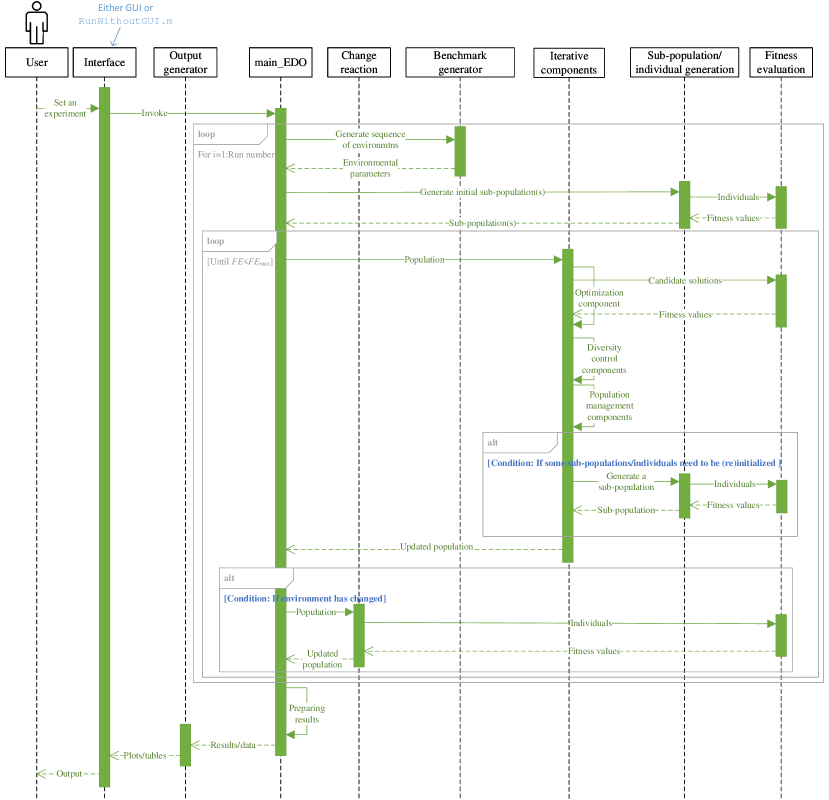
Figure 1. A general sequence diagram of running an EDOA in EDOLAB.

Afterward, the EDOA’s main loop is executed. In each iteration, the iterative components of the EDOA, such as the optimizer (e.g., PSO or DE), diversity control, and population management (Yazdani et al., 2020a), are executed by calling the iterative components function (e.g., $\mathtt{IterativeComponents\_AmQSO.m}$). In many EDOAs with adaptive sub-population number and/or population size, some new individuals/sub-populations are generated when some conditions are met (Yazdani et al., 2021b). Besides, some diversity and population management components of EDOAs also may require reinitializing some sub-populations/individuals. Therefore, in each iteration, if some sub-populations/individuals need to be (re)initialized, the sub-population/individual generation function is called. Thereafter, the updated population is returned to the main EDOA function. At the end of each iteration, if the environment has changed, the change reaction components are called (e.g., $\mathtt{ChangeReaction\_AmQSO.m}$). The main loop of the EDOA continues until the number of fitness evaluations ($FE$) reaches their predefined maximum value ($FE_{\mathrm{max}}$). The aforementioned procedure repeats $\mathtt{RunNumber}$ times. Afterward, the results are prepared (e.g., performance indicator calculation). The results, as well as some gathered data, are then sent to output generator functions that are responsible for generating output plots, tables, and files. Finally, the output tables and figures are returned to the interface.

3.2. Running

As stated before, EDOLAB can be used either with or without GUI. In the following, we describe these two ways.

3.2.1. Using EDOLAB via GUI

As stated before, EDOLAB’s GUI is developed using MATLAB App Designer and can be accessed by executing $\mathtt{GUI.MLAPP}$ or $\mathtt{RunWithGUI.m}$ in the root directory of EDOLAB. EDOLAB’s GUI contains two modules –Experimentation and Education– which are explained below.

Experimentation module

The experimentation module is intended to be used for performing experiments. Figure 2 shows the interface of the experimentation module. In this module, the user can select the algorithm (EDOA) and benchmark generator. Furthermore, the user can set the parameters of the benchmark generator to generate the desired problem instance. Note that EDOLAB’s GUI does not provide any facility for changing the parameter settings of EDOAs. In fact, EDOAs generally contain many parameters that are different from one algorithm to another based on the components used in their structures. Consequently, adding the facility for defining the parameters of different EDOAs in the GUI would make it complex, hard to use, and confusing. In EDOLAB, the parameters of the EDOAs are set according to the suggested values in their original references. Our investigations also indicate that these EDOAs show their best performance with those suggested settings. Those users who are interested in performing sensitivity analysis on the parameters of EDOAs can change their values in the source codes.

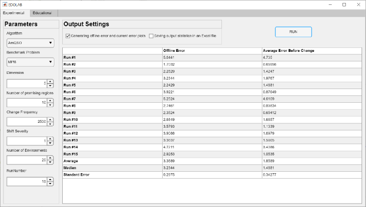
Figure 2. The experimentation module of EDOLAB.

As can be seen in Figure 2, the run number and some main parameters of the benchmark generators, including dimension, number of promising regions, change frequency, shift severity, and the number of environments that are common between MPB, GMPB, and FPs, can be set in the GUI. Type and suggested values for these parameters are shown in Table 2. Note that in the majority of works in the field, only the dimension, number of promising regions, change frequency, and shift severity values in the benchmark generators are modified in order to generate different problem instances. Finally, “output settings” need to be configured, where using two check boxes, the user can opt whether he/she requires an output figure containing the offline error and current error plots and an Excel file containing the output results and statistics.

Table 2. Type and suggested values for the main parameters of the benchmark generators in EDOLAB.

Parameter	Name in the source code	Type	Suggested values
Dimension	$\mathtt{Problem.Dimension}$	Positive integer	$\in\{1,2,5,10\}$$\star$
Number of promising regions	$\mathtt{Problem.PeakNumber}$	Positive integer	$\in\{10,25,50,100\}$
Change frequency	$\mathtt{Problem.ChangeFrequency}$	Positive integer	$\in\{500,1000,2500,5000\}$
Shift severity	$\mathtt{Problem.ShiftSeverity}$	Non-negative real valued	$\in\{1,2,5\}$
Number of environments	$\mathtt{Problem.EnvironmentNumber}$	Positive integer	$100$$\dagger$

• These are suggested values for the experimentation module. In the education module, the dimension can only be set to two.

• For the sake of understandability, the number of environments is suggested to set between 10 and 20 in the education module.

After finishing the experiment configuration, it can be started by pressing the $\mathtt{RUN}$ button in the top-right of the experimentation module interface. Depending on the complexity of the chosen EDOA and the configured problem instance, the experiment can take a long time to finish. It is worth mentioning that due to the complexity of the EDOAs and dynamic benchmark generators, runs in this field generally take a longer time in comparison to some other sub-fields of evolutionary computation with similar problem dimensionalities, such as evolutionary static optimization and evolutionary multi-objective optimization. To show experiment running progress in EDOLAB, the current run number and environment are displayed in the MATLAB Command Window. Once the experiment is carried out, the results of all runs as well as their average, median, and standard error values are displayed. In addition, if the user has ticked the related check-box, the aforementioned information, along with the values of the benchmark’s main parameters, is saved in an Excel file in the $\mathtt{Results}$ folder. The Excel file name includes the EDOA and benchmark names, as well as the date and time of the experiment ($\mathtt{EDOA\_Benchmark\_DateTime.xlsx}$). The statistics and results stored in the Excel files can then be used for performing desirable statistical analysis for comparing results using MATLAB or other applications. An Excel file generated by EDOLAB is shown in Figure 3. Furthermore, a figure containing the plots of offline and current errors over time is generated (if the user has ticked the related check-box). An example of the output plots is given in Figure 4.

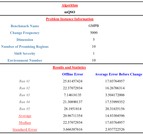
Figure 3. An Excel output table generated by EDOLAB’s $\mathtt{OutputExcel.m}$ function.

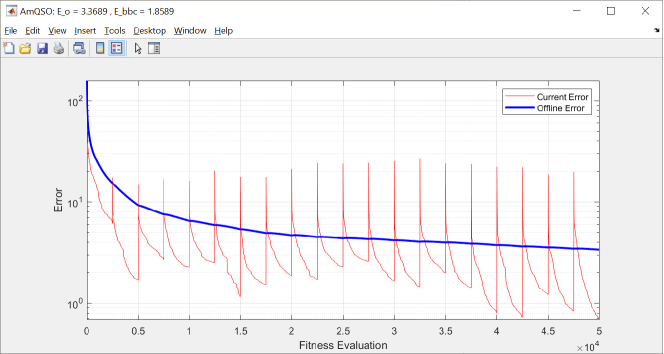
Figure 4. An output figure of an experimentation in EDOLAB. This figure depicts the plots of offline and current errors over time. The plots are the average of all runs.

Education module

Using the education module, the user can visually observe the current environment, environmental changes, and the position and behavior of the individuals over time. Figure 5 shows the education module of EDOLAB. In the left part of the interface, the user can configure an experiment that is similar to the experimentation module. However, only 2-dimensional problem instances are considered in the education module since we intend to visualize the problem space and individuals. After configuring the experiment and pressing the $\mathtt{RUN}$ button, the experiment is run, and the environmental parameters and individuals’ positions over time are archived, which takes time (the waiting time depends on the CPU, the chosen EDOA, and the benchmark settings). After finishing the run, the archived information is sent to the education module interface.

Figure 5. The education module of EDOLAB.

Using the archived information, the education module provides a video for showing the environments and positions of individuals over time. As shown in Figure 5, a 2-dimensional contour plot is used for this purpose. In the contour plot, the center position of each visible promising region is marked with a black circle, the global optimum position is marked with a black pentagram, and individuals are marked with green filled circles. The positions of individuals shown in the contour plot are updated every iteration. The contour plot is also updated after each environmental change. In addition to the contour plot, the current error plot and the current environment number are shown to provide additional information for improving the understandability of the behaviors of the problem and EDOA.

By monitoring the individuals’ positions, the search space/environment, current environment number, and the current error plot over time, the user can observe the performance of exploration, exploitation, and tracking in each environment. Moreover, the capability of the components of EDOAs from some other aspects such as establishing mutual exclusion in the promising regions (Blackwell and Branke, 2006), generating new sub-populations (Blackwell et al., 2008), promising regions coverage, randomization based mechanisms for increasing global diversity, and change reaction can also be observed in the education module.

Note that unlike the experimentation module, which uses identical random seed numbers for benchmark generators in all experiments, different random numbers are used in the education module for each run. Therefore, in each run of the education module, the user can observe the behavior and performance of the EDOA in different problem instances.

3.2.2. Using EDOLAB without GUI

EDOLAB can also be used without the GUI, which offers more advanced and flexible options. To this end, the user needs to work with the source codes of EDOLAB. Interacting with the source codes of EDOLAB makes the user able to (1) change the parameter settings of the EDOAs, (2) modify or deactivate some components of the EDOAs, and (3) alter the values of all parameters of benchmarks. To improve the readability, understandability, and navigation over the source codes of EDOLAB, we have:

• divided all the codes to sections using $\%\%$ command and provided a descriptive header for each section. Each section includes several lines of codes that are related to each other. For example, a section can include a group of lines that implements a component (e.g., exclusion (Blackwell and Branke, 2006)), initializes EDOA’s parameters, or prepares output values,

• chosen meaningful and descriptive names for all the structures, parameters, and functions in the EDOLAB, and

• added helpful comments to many lines.

For running an EDOA in EDOLAB without the GUI, the user needs to interact with the $\mathtt{RunWithoutGUI.m}$ file in the root directory of EDOLAB. In $\mathtt{RunWithoutGUI.m}$, the user can choose the EDOA and benchmark, and set the benchmark’s main parameters (see Table 2). To select an EDOA and a benchmark, the user must set $\mathtt{AlgorithmName}$ to the name of the EDOA (e.g., $\mathtt{AlgorithmName}\;=\;^{\prime}\mathtt{mQSO}^{\backprime}$) and $\mathtt{BenchmarkName}$ to the name of the benchmark (e.g., $\mathtt{BenchmarkName}\;=\;^{\prime}\mathtt{GMPB}^{\backprime}$), respectively.

The user can also choose either the experimentation or education module in $\mathtt{RunWithoutGUI.m}$. Similar to EDOLAB’s education module in the GUI (see Figure 5), the contour plots of the environments, the positions of individuals, and the current error over time are shown when the education module is chosen in $\mathtt{RunWithoutGUI.m}$. In $\mathtt{RunWithoutGUI.m}$, EDOLAB’s education module is activated if the user sets $\mathtt{VisualizationOverOptimization=1}$.

If $\mathtt{VisualizationOverOptimization=0}$, the experimentation module is activated. When the user plans to use the experimentation module, he/she can configure the outputs. To this end, $\mathtt{OutputFigure}$ can be set to 1 if he/she requires offline and current error plots as visualized outputs of the experiment (see Figure 4). In addition, by setting $\mathtt{GeneratingExcelFile=1}$, an excel file containing output statistics and results is saved in the $\mathtt{Results}$ folder. As stated before, archived results in the Excel files can be later used for performing statistical analysis.

The parameters of the chosen EDOA can also be changed in its main function (e.g., $\mathtt{main\_mQSO.m}$) which can be found in the EDOA’s sub-folder. As stated before, the default values of these parameters are set according to the values suggested in their original references. The code lines related to the EDOA’s parameters initialization can be found in section $\mathtt{\%\%~{}Initializing~{}Optimizer}$ of the main function of the EDOA. A structure named $\mathtt{Optimizer}$ contains all the parameters of the EDOA.

In addition to the main parameters of the benchmark generators used in EDOLAB, which are listed in Table 2, each benchmark has several other parameters. Usually, researchers only change the main parameters of the benchmarks to generate different problem instances. However, some may desire to investigate the performance of EDOAs on problem instances with some particular characteristics. In this case, the user can change other parameter values of the chosen benchmark generator in $\mathtt{BenchmarkGenerator\_Benchmark.m}$. For example, Table 3 shows the parameters of GMPB whose values can be altered by the user in $\mathtt{BenchmarkGenerator\_GMPB.m}$ located in $\mathtt{EDOLAB\backslash Benchmark\backslash GMPB}$.

Table 3. Parameters of GMPB that can be changed by the user to generate problem instances with different morphological and dynamical characteristics.

Parameter	Name in the source code	Suggested value(s)
Dimension$\dagger$	$\mathtt{Problem.Dimension}$	$\in\{1,2,5,10\}$
Numbers of promising regions$\dagger$	$\mathtt{Problem.PeakNumber}$	$\in\{10,25,50,100\}$
Change frequency$\dagger$	$\mathtt{Problem.ChangeFrequency}$	$\in\{500,1000,2500,5000\}$
Shift severity$\dagger$	$\mathtt{Problem.ShiftSeverity}$	$\in\{1,2,5\}$
Number of environments$\dagger$	$\mathtt{Problem.EnvironmentNumber}$	$100$
Height severity	$\mathtt{Problem.HeightSeverity}$	7
Width severity	$\mathtt{Problem.WidthSeverity}$	1
Irregularity parameter $\tau$ severity	$\mathtt{Problem.TauSeverity}$	0.05
Irregularity parameter $\eta$ severity	$\mathtt{Problem.EtaSeverity}$	2
Angle severity	$\mathtt{Problem.AngleSeverity}$	$\pi/9$
Search range upper bound	$\mathtt{Problem.MaxCoordinate}$	$50$
Search range lower bound	$\mathtt{Problem.MinCoordinate}$	$-50$
Maximum height	$\mathtt{Problem.MaxHeight}$	$70$
Minimum height	$\mathtt{Problem.MinHeight}$	$30$
Maximum width	$\mathtt{Problem.MaxWidth}$	$12$
Minimum width	$\mathtt{Problem.MinWidth}$	$1$
Maximum angle	$\mathtt{Problem.MaxAngle}$	$\pi$
Minimum angle	$\mathtt{Problem.MinAngle}$	$-\pi$
Maximum irregularity parameter $\tau$	$\mathtt{Problem.MaxTau}$	$0.4$
Minimum irregularity parameter $\tau$	$\mathtt{Problem.MinTau}$	$0$
Maximum irregularity parameter $\eta$	$\mathtt{Problem.MaxEta}$	$25$
Minimum irregularity parameter $\eta$	$\mathtt{Problem.MinEta}$	$10$

• These are commonly used parameters to generate different problem instances with various characteristics. As stated before, these parameters are common among the benchmark generators of EDOLAB and can be either set in the GUI or $\mathtt{RunWithoutGUI.m}$.

Once the configurations are done, the user can run $\mathtt{RunWithoutGUI.m}$ to start the experiment. The run progress information, including the current run number and the current environment number, is shown in the MATLAB Command Window. After finishing the experiment, its results are shown in the MATLAB Command Window.

3.3. Extension

Users can extend EDOLAB since it is an open-source platform. In the following, we describe how users can add new benchmark generators, performance indicators, and EDOAs to EDOLAB.

3.3.1. Adding a benchmark generator

Assume that the user intends to add a new benchmark called ABC. First, the user needs to create a new sub-folder in the $\mathtt{Benchmark}$ folder and name it ABC. Two functions named $\mathtt{fitness\_ABC.m}$ and $\mathtt{BenchmarkGenerator\_ABC.m}$ are then needed to be added into the ABC sub-folder.

In $\mathtt{BenchmarkGenerator\_ABC.m}$, the user needs to define and initialize all the parameters of the new benchmark in a structure named $\mathtt{Problem}$, similar to the way that we have defined the parameters of the existing benchmark generators in EDOLAB. Thereafter, the environmental parameters of all the environments need to be generated in $\mathtt{BenchmarkGenerator\_ABC.m}$. Note that all environmental and control parameters of the ABC must be stored in the $\mathtt{Problem}$ structure.

The other function –$\mathtt{fitness\_ABC.m}$– will contain the code of ABC’s baseline function. Note that the inputs and outputs of $\mathtt{BenchmarkGenerator\_ABC.m}$ and $\mathtt{fitness\_ABC.m}$ must be similar to those of EDOLAB’s current benchmarks. No changes to other functions are required, and ABC is automatically added to the list of benchmarks in the GUI and can be accessed via $\mathtt{RunWithoutGUI.m}$.

3.3.2. Adding a performance indicator

Generally, the information required for calculating the performance indicators in the DOP literature is collected over time, e.g., at the end of each environment (Trojanowski and Michalewicz, 1999), every fitness evaluation (Branke and Schmeck, 2003), or when the solution is deployed in each environment (Yazdani, 2018). In EDOLAB, this information is collected in $\mathtt{fitness.m}$ and archived in the $\mathtt{Problem}$ structure. To add a new performance indicator, in the first step, the user needs to add the code that collects the required information in $\mathtt{fitness.m}$ and store it in $\mathtt{Problem}$ structure. Then, the code for calculating the performance indicator needs to be added in section $\mathtt{\%\%~{}Performance~{}indicator~{}calculation}$ of the main function of EDOA (e.g., $\mathtt{main\_mQSO.m}$). In addition, the results of the newly added performance indicator must be added to the outputs in section $\mathtt{\%\%~{}Output~{}preparation}$ at the bottom of the main function of EDOA.

3.3.3. Adding an EDOA

To add a new EDOA to EDOLAB, its source code must be slightly modified to become compatible with EDOLAB. To this end, the user needs to consider the following points:

• First, a sub-folder, which must be named similarly to the EDOA, needs to be created inside the $\mathtt{Algorithm}$ folder. Then, the functions of the new EDOA need to be added to this sub-folder.

• To run the new EDOA, it must be invoked by $\mathtt{RunWithoutGUI.m}$. Thus, the user needs to consider the inputs and outputs of the main function of the EDOA when it is invoked by $\mathtt{RunWithoutGUI.m}$.

• In the main function of the new EDOA, first, $\mathtt{BenchmarkGenerator.m}$ needs to be called for generating the problem instance.

• The code that generates and collects the information related to the education module needs to be added to the main loop of EDOA. This part of the code can be found in section $\mathtt{\%\%~{}Visualization~{}for~{}education~{}module}$ of the main function of EDOAs.

• Use $\mathtt{fitness.m}$ for evaluating fitness of solutions.

• To make the newly added EDOA accessible via EDOLAB, its main function file must be named as $\mathtt{main\_EDOA.m}$.

For example, if the name of the new EDOA is XYZ, then the sub-folder needs to be named XYZ and the main function file inside this sub-folder must be named as $\mathtt{main\_XYZ.m}$. Thereafter, the name of the new EDOA will be automatically added to the list of EDOAs in both modules of the GUI. In addition, by setting $\mathtt{AlgorithmName}\;=\;^{\prime}\mathtt{XYZ}^{\backprime}$, this algorithm can be run using $\mathtt{RunWithoutGUI.m}$.

4. Conclusion

Evolutionary dynamic optimization methods (EDOAs) and dynamic benchmark generators are usually complex. The complexity of these algorithms and benchmark generators makes re-implementing them hard and error-prone. During the last two decades, the lack of publicly available source codes for many EDOAs and dynamic benchmark generators has caused a significant challenge for researchers in reproducing the results for experimentation and comparisons. To address this issue, this paper has introduced an open-source MATLAB optimization platform for evolutionary dynamic optimization, called Evolutionary Dynamic Optimization Laboratory (EDOLAB). The main purposes of developing EDOLAB are to help the researchers, in particular the less experienced ones, to understand how the EDOAs work and what are the morphological and dynamical characteristics of the dynamic benchmark problem instances, and to facilitate the experimentation and comparison of their EDOAs with various peer algorithms. The former and latter purposes are achieved by the education and experimentation modules of EDOLAB, respectively. The initial release of EDOLAB includes 25 EDOAs, three parametric and highly configurable benchmark generators, and two commonly used performance indicators. In this paper, we have described the technical aspects of EDOLAB, including its architecture, the steps of running EDOLAB with and without the GUI, the education and experimentation modules, and the ways of expanding EDOLAB by adding new EDOAs, benchmark generators, and performance indicators.

As future work, more EDOAs, in particular the state-of-the-art ones, should be added to EDOLAB to further enrich its library. In addition, covering other important sub-fields of dynamic optimization including dynamic multi-objective optimization (Jiang et al., 2022; Raquel and Yao, 2013), large-scale dynamic optimization (Yazdani et al., 2019; Bai et al., 2022), dynamic multimodal optimization (Lin et al., 2022; Luo et al., 2019), dynamic constrained optimization (Nguyen and Yao, 2012; Bu et al., 2016), and robust optimization over time (Fu et al., 2015; Yu et al., 2010; Jin et al., 2013) in EDOLAB is an important future work.

References

- (1)
- Bai et al. (2022) Hui Bai, Ran Cheng, Danial Yazdani, Kay Chen Tan, and Yaochu Jin. Early access, 2022. Evolutionary Large-Scale Dynamic Optimization Using Bilevel Variable Grouping. IEEE Transactions on Cybernetics (Early access, 2022).
- Bentley and Friedman (1979) Jon Louis Bentley and Jerome H. Friedman. 1979. Data Structures for Range Searching. Comput. Surveys 11, 4 (1979), 397–409.
- Blackwell and Branke (2006) Tim Blackwell and Juergen Branke. 2006. Multiswarms, exclusion, and anti-convergence in dynamic environments. IEEE Transactions on Evolutionary Computation 10, 4 (2006), 459–472.
- Blackwell et al. (2008) Tim Blackwell, Juergen Branke, and Xiaodong Li. 2008. Particle swarms for dynamic optimization problems. In Swarm Intelligence: Introduction and Applications, Christian Blum and Daniel Merkle (Eds.). Springer Lecture Notes in Computer Science, 193–217.
- Bonyadi and Michalewicz (2017) Mohammad Reza Bonyadi and Zbigniew Michalewicz. 2017. Particle swarm optimization for single objective continuous space problems: a review. , 54 pages.
- Branke (1999) Juergen Branke. 1999. Memory enhanced evolutionary algorithms for changing optimization problems. In IEEE Congress on Evolutionary Computation, Vol. 3. IEEE, 1875–1882.
- Branke (2012) Juergen Branke. 2012. Evolutionary optimization in dynamic environments. Vol. 3. Springer Science & Business Media.
- Branke and Schmeck (2003) Juergen Branke and Hartmut Schmeck. 2003. Designing Evolutionary Algorithms for Dynamic Optimization Problems. In Advances in Evolutionary Computing, A. Ghosh and S. Tsutsui (Eds.). Springer Natural Computing Series, 239–262.
- Brest et al. (2006) Janez Brest, Sao Greiner, Borko Boskovic, Marjan Mernik, and Viljem Zumer. 2006. Self-Adapting Control Parameters in Differential Evolution: A Comparative Study on Numerical Benchmark Problems. IEEE Transactions on Evolutionary Computation 10, 6 (2006), 646–657.
- Bu et al. (2016) Chenyang Bu, Wenjian Luo, and Lihua Yue. 2016. Continuous dynamic constrained optimization with ensemble of locating and tracking feasible regions strategies. IEEE Transactions on Evolutionary Computation 21, 1 (2016), 14–33.
- Das and Suganthan (2010) Swagatam Das and Ponnuthurai Nagaratnam Suganthan. 2010. Differential evolution: A survey of the state-of-the-art. IEEE transactions on evolutionary computation 15, 1 (2010), 4–31.
- Du Plessis and Engelbrecht (2012) Mathys C. Du Plessis and Andries P. Engelbrecht. 2012. Using competitive population evaluation in a differential evolution algorithm for dynamic environments. European Journal of Operational Research 218, 1 (2012), 7–20.
- du Plessis and Engelbrecht (2013) Mathys C. du Plessis and Andries P. Engelbrecht. 2013. Differential evolution for dynamic environments with unknown numbers of optima. Journal of Global Optimization 55, 1 (2013), 73–99.
- Duhain (2012) Julien Georges Omer Louis Duhain. 2012. Particle swarm optimisation in dynamically changing environments - an empirical study. Master’s thesis. University of Pretoria, Pretoria, South Africa.
- Eberhart and Shi (2001) Russell C. Eberhart and Yuhui Shi. 2001. Comparing inertia weights and constriction factors in particle swarm optimization. In Congress on Evolutionary Computation, Vol. 1. IEEE, 84–88.
- Fu et al. (2015) Haobo Fu, Bernhard Sendhoff, Ke Tang, and Xin Yao. 2015. Robust optimization over time: Problem difficulties and benchmark problems. IEEE Transactions on Evolutionary Computation 19, 5 (2015), 731–745.
- Gandomi and Yang (2012) Amir Hossein Gandomi and Xin-She Yang. 2012. Evolutionary boundary constraint handling scheme. Neural Computing and Applications 21, 6 (2012), 1449–1462.
- Helwig et al. (2012) Sabine Helwig, Juergen Branke, and Sanaz Mostaghim. 2012. Experimental analysis of bound handling techniques in particle swarm optimization. IEEE Transactions on Evolutionary computation 17, 2 (2012), 259–271.
- Herring et al. (2022) Daniel Herring, Michael Kirley, and Xin Yao. 2022. Reproducibility and Baseline Reporting for Dynamic Multi-Objective Benchmark Problems. In Proceedings of the Genetic and Evolutionary Computation Conference (Boston, Massachusetts) (GECCO ’22). Association for Computing Machinery, New York, NY, USA, 529–537.
- Hu and Eberhart (2002) Xiaohui Hu and Russell C. Eberhart. 2002. Adaptive particle swarm optimization: detection and response to dynamic systems. In Congress on Evolutionary Computation, Vol. 2. IEEE, 1666–1670.
- Jiang et al. (2022) Shouyong Jiang, Juan Zou, Shengxiang Yang, and Xin Yao. Early Access, 2022. Evolutionary Dynamic Multi-Objective Optimisation: A survey. Comput. Surveys (Early Access, 2022).
- Jin and Branke (2005) Yaochu Jin and Juergen Branke. 2005. Evolutionary optimization in uncertain environments-a survey. IEEE Transactions on evolutionary computation 9, 3 (2005), 303–317.
- Jin et al. (2013) Yaochu Jin, Ke Tang, Xin Yu, Bernhard Sendhoff, and Xin Yao. 2013. A framework for finding robust optimal solutions over time. Memetic Computing 5, 1 (2013), 3–18.
- Kaddani et al. (2017) Sami Kaddani, Daniel Vanderpooten, Jean-Michel Vanpeperstraete, and Hassene Aissi. 2017. Weighted sum model with partial preference information: application to multi-objective optimization. European Journal of Operational Research 260, 2 (2017), 665–679.
- Kamosi et al. (2010) Masoud Kamosi, Ali Baradaran Hashemi, and Mohommad Reza Meybodi. 2010. A hibernating multi-swarm optimization algorithm for dynamic environments. In Nature and Biologically Inspired Computing. IEEE, 363–369.
- Kordestani et al. (2019) Javidan Kazemi Kordestani, Mohammad Reza Meybodi, and Amir Masoud Rahmani. 2019. A note on the exclusion operator in multi-swarm PSO algorithms for dynamic environments. Connection Science (2019), 1–25.
- Li et al. (2016) Changhe Li, Trung Thanh Nguyen, Ming Yang, Michalis Mavrovouniotis, and Shengxiang Yang. 2016. An Adaptive Multipopulation Framework for Locating and Tracking Multiple Optima. IEEE Transactions on Evolutionary Computation 20, 4 (2016), 590–605.
- Li et al. (2018) Changhe Li, Trung Thanh Nguyen, Sanyou Zeng, Ming Yang, and Min Wu. 2018. An Open Framework for Constructing Continuous Optimization Problems. IEEE Transactions on Cybernetics 49, 6 (2018).
- Li and Yang (2012) Changhe Li and Shengxiang Yang. 2012. A General Framework of Multipopulation Methods With Clustering in Undetectable Dynamic Environments. IEEE Transactions on Evolutionary Computation 16, 4 (2012), 556–577.
- Li et al. (2008) Changhe Li, Shengxiang Yang, Trung Thanh Nguyen, E. Ling Yu, Xin Yao, Yaochu Jin, Hans-Georg Beyer, and Ponnuthurai N. Suganthan. 2008. Benchmark Generator for CEC’2009 Competition on Dynamic Optimization. Technical Report. Center for Computational Intelligence.
- Li et al. (2014) Changhe Li, Shengxiang Yang, and Ming Yang. 2014. An Adaptive Multi-Swarm Optimizer for Dynamic Optimization Problems. Evolutionary Computation 22, 4 (2014), 559–594.
- Liang et al. (2005) Jing Liang, Ponnuthurai N. Suganthan, and Kalyan Deb. 2005. Novel composition test functions for numerical global optimization. In Swarm Intelligence Symposium. IEEE, 68–75.
- Lin et al. (2022) Xin Lin, Wenjian Luo, Peilan Xu, Yingying Qiao, and Shengxiang Yang. 2022. PopDMMO: A general framework of population-based stochastic search algorithms for dynamic multimodal optimization. Swarm and Evolutionary Computation 68 (2022), 101011.
- Lung and Dumitrescu (2007) Rodica Ioana Lung and Dumitru Dumitrescu. 2007. A collaborative model for tracking optima in dynamic environments. In Congress on Evolutionary Computation. IEEE, 564–567.
- Luo et al. (2019) Wenjian Luo, Xin Lin, Tao Zhu, and Peilan Xu. 2019. A clonal selection algorithm for dynamic multimodal function optimization. Swarm and Evolutionary Computation 50 (2019), 100459.
- Luo et al. (2018) Wenjian Luo, Juan Sun, Chenyang Bu, and Ruikang Yi. 2018. Identifying Species for Particle Swarm Optimization under Dynamic Environments. In Symposium Series on Computational Intelligence (SSCI). IEEE, 1921–1928.
- Luo et al. (2017) Wenjian Luo, Bin Yang, Chenyang Bu, and Xin Lin. 2017. A Hybrid Particle Swarm Optimization for High-Dimensional Dynamic Optimization. In Simulated Evolution and Learning, Yuhui Shi et al. (Ed.). Springer International Publishing, Cham, 981–993.
- Marler and Arora (2010) Timothy Marler and Jasbir S. Arora. 2010. The weighted sum method for multi-objective optimization: new insights. Structural and multidisciplinary optimization 41, 6 (2010), 853–862.
- Mendes and Mohais (2005) Rui Mendes and Arvind Mohais. 2005. DynDE: a differential evolution for dynamic optimization problems. In Congress on Evolutionary Computation, Vol. 3. IEEE, 2808–2815.
- Mezura-Montes and Coello (2011) Efrén Mezura-Montes and Carlos A Coello Coello. 2011. Constraint-handling in nature-inspired numerical optimization: past, present and future. Swarm and Evolutionary Computation 1, 4 (2011), 173–194.
- Nguyen (2011) Trung Thanh Nguyen. 2011. Continuous dynamic optimisation using evolutionary algorithms. Ph.D. Dissertation. University of Birmingham.
- Nguyen et al. (2012) Trung Thanh Nguyen, Shengxiang Yang, and Juergen Branke. 2012. Evolutionary dynamic optimization: A survey of the state of the art. Swarm and Evolutionary Computation 6 (2012), 1 – 24.
- Nguyen and Yao (2012) Trung Thanh Nguyen and Xin Yao. 2012. Continuous dynamic constrained optimization—The challenges. IEEE Transactions on Evolutionary Computation 16, 6 (2012), 769–786.
- Parrott and Li (2006) Daniel Parrott and Xiaodong Li. 2006. Locating and tracking multiple dynamic optima by a particle swarm model using speciation. IEEE Transactions on Evolutionary Computation 10, 4 (2006), 440–458.
- Raquel and Yao (2013) Carlo Raquel and Xin Yao. 2013. Dynamic multi-objective optimization: a survey of the state-of-the-art. In Evolutionary computation for dynamic optimization problems. Springer, 85–106.
- Suganthan et al. (2005) Ponnuthurai N. Suganthan, Nikolaus Hansen, Jing Liang, Kalyan Deb, Ying ping Chen, Anne Auger, and S Tiwari. 2005. Problem definitions and evaluation criteria for the CEC 2005 special session on real-parameter optimization. Technical Report. Nanyang Technological University.
- Thomsen (2004) Rene Thomsen. 2004. Multimodal optimization using crowding-based differential evolution. In Congress on Evolutionary Computation, Vol. 2. IEEE, 1382–1389.
- Trojanowski and Michalewicz (1999) Krzysztof Trojanowski and Zbigniew Michalewicz. 1999. Searching for optima in non-stationary environments. In Congress on Evolutionary Computation, Vol. 3. 1843–1850.
- Wang et al. (2007) Hongfeng Wang, Dingwei Wang, and Shengxiang Yang. 2007. Triggered Memory-Based Swarm Optimization in Dynamic Environments. In Applications of Evolutionary Computing, Mario Giacobini (Ed.). Springer Berlin Heidelberg, 637–646.
- Yang and Li (2010) Shengxiang Yang and Changhe Li. 2010. A Clustering Particle Swarm Optimizer for Locating and Tracking Multiple Optima in Dynamic Environments. IEEE Transactions on Evolutionary Computation 14, 6 (2010), 959–974.
- Yazdani (2018) Danial Yazdani. 2018. Particle swarm optimization for dynamically changing environments with particular focus on scalability and switching cost. Ph.D. Dissertation. Liverpool John Moores University, Liverpool, UK.
- Yazdani et al. (2021a) Danial Yazdani, Juergen Branke, Mohammad Nabi Omidvar, Xiaodong Li, Changhe Li, Michalis Mavrovouniotis, Trung Thanh Nguyen, Shengxiang Yang, and Xin Yao. 2021a. IEEE CEC 2022 competition on dynamic optimization problems generated by generalized moving peaks benchmark. arXiv preprint arXiv:2106.06174 (2021).
- Yazdani et al. (2018a) Danial Yazdani, Juergen Branke, Mohammad Nabi Omidvar, Trung Thanh Nguyen, and Xin Yao. 2018a. Changing or Keeping Solutions in Dynamic Optimization Problems with Switching Costs. In Proceedings of the Genetic and Evolutionary Computation Conference. ACM, 1095–1102.
- Yazdani et al. (2020a) Danial Yazdani, Ran Cheng, Cheng He, and Juergen Branke. 2020a. Adaptive Control of Subpopulations in Evolutionary Dynamic Optimization. IEEE Transactions on Cybernetics (2020).
- Yazdani et al. (2021b) Danial Yazdani, Ran Cheng, Donya Yazdani, Juergen Branke, Yaochu Jin, and Xin Yao. 2021b. A Survey of Evolutionary Continuous Dynamic Optimization Over Two Decades – Part A. IEEE Transactions on Evolutionary Computation (2021).
- Yazdani et al. (2021c) Danial Yazdani, Ran Cheng, Donya Yazdani, Juergen Branke, Yaochu Jin, and Xin Yao. 2021c. A Survey of Evolutionary Continuous Dynamic Optimization Over Two Decades – Part B. IEEE Transactions on Evolutionary Computation (2021).
- Yazdani et al. (2013) Danial Yazdani, Babak Nasiri, Alireza Sepas-Moghaddam, and Mohammad Reza Meybodi. 2013. A novel multi-swarm algorithm for optimization in dynamic environments based on particle swarm optimization. Applied Soft Computing 13, 4 (2013), 2144–2158.
- Yazdani et al. (2018b) Danial Yazdani, Trung Thanh Nguyen, and Juergen Branke. 2018b. Robust optimization over time by learning problem space characteristics. IEEE Transactions on Evolutionary Computation 23, 1 (2018), 143–155.
- Yazdani et al. (2017) Danial Yazdani, Trung Thanh Nguyen, Juergen Branke, and Jin Wang. 2017. A New Multi-swarm Particle Swarm Optimization for Robust Optimization Over Time. In Applications of Evolutionary Computation, Giovanni Squillero and Kevin Sim (Eds.). Springer International Publishing, 99–109.
- Yazdani et al. (2019) Danial Yazdani, Mohammad Nabi Omidvar, Juergen Branke, Trung Thanh Nguyen, and Xin Yao. 2019. Scaling Up Dynamic Optimization Problems: A Divide-and-Conquer Approach. IEEE Transaction on Evolutionary Computation (2019).
- Yazdani et al. (2020b) Danial Yazdani, Mohammad Nabi Omidvar, Ran Cheng, Juergen Branke, Trung Thanh Nguyen, and Xin Yao. 2020b. Benchmarking Continuous Dynamic Optimization: Survey and Generalized Test Suite. IEEE Transactions on Cybernetics (2020), 1 – 14.
- Yazdani et al. (2023a) Danial Yazdani, Mohammad Nabi Omidvar, Donya Yazdani, Jürgen Branke, Trung Thanh Nguyen, Amir H Gandomi, Yaochu Jin, and Xin Yao. 2023a. Robust Optimization Over Time: A Critical Review. IEEE Transactions on Evolutionary Computation (2023).
- Yazdani et al. (2022) Danial Yazdani, Donya Yazdani, Juergen Branke, Mohammad Nabi Omidvar, Amir Hossein Gandomi, and Xin Yao. 2022. Robust Optimization Over Time by Estimating Robustness of Promising Regions. IEEE Transactions on Evolutionary Computation (2022).
- Yazdani et al. (2023b) Delaram Yazdani, Danial Yazdani, Donya Yazdani, Mohammad Nabi Omidvar, Amir H. Gandomi, and Xin Yao. 2023b. A Species-Based Particle Swarm Optimization with Adaptive Population Size and Deactivation of Species for Dynamic Optimization Problems. ACM Transactions on Evolutionary Learning Optimization (2023), Early access. https://doi.org/10.1145/3604812
- Yu et al. (2010) Xin Yu, Yaochu Jin, Ke Tang, and Xin Yao. 2010. Robust optimization over time—a new perspective on dynamic optimization problems. In IEEE Congress on evolutionary computation. IEEE, 1–6.