Masked Autoencoders are Efficient Class Incremental Learners

Abstract

Class Incremental Learning (CIL) aims to sequentially learn new classes while avoiding catastrophic forgetting of previous knowledge. We propose to use Masked Autoencoders (MAEs) as efficient learners for CIL. MAEs were originally designed to learn useful representations through reconstructive unsupervised learning, and they can be easily integrated with a supervised loss for classification. Moreover, MAEs can reliably reconstruct original input images from randomly selected patches, which we use to store exemplars from past tasks more efficiently for CIL. We also propose a bilateral MAE framework to learn from image-level and embedding-level fusion, which produces better-quality reconstructed images and more stable representations. Our experiments confirm that our approach performs better than the state-of-the-art on CIFAR-100, ImageNet-Subset, and ImageNet-Full. The code is available at https://github.com/scok30/MAE-CIL.

1 Introduction

Deep learning has had a broad and deep impact on most computer vision tasks over the last ten years. Given the way humans learn continually in their lifespan, it is natural to expect models also to be able to accumulate knowledge and build on past experiences to adapt to new tasks incrementally. The real world is very dynamic, leading to varying data distributions over time, while deep models tend to catastrophically forget old tasks when learning new ones [26].

Class Incremental Learning (CIL) aims to learn new classification tasks sequentially while avoiding catastrophic forgetting [2, 25]. CIL approaches can be roughly divided into three categories [5], , Rehearsal-based methods [13, 29, 31], Regularization-based methods [15, 17], and Architecture-based methods [1, 23, 24]. Among them, Rehearsal-based methods achieve state-of-the-art performance by storing exemplars from past tasks or generating synthetic samples for replay.

Normally, only a fixed size of memory is allowed during incremental learning. Therefore, it limits the stored exemplars from past tasks. Other works exploit generative networks [35, 38, 43] (e.g., GANs) to synthesize samples from old tasks for replay. Although they can generate replay data to mitigate forgetting, a typical drawback is the quality of generated images, and that forgetting can also happen in generative models. In this work, we introduce Masked Autoencoders (MAEs) [11] as a base model to replay. It allows efficient exemplar storage by only requiring a small subset of patches to reconstruct whole images. Therefore, we can store more exemplars with the same amount of limited memory as other exemplar-based approaches. Compared to previous generative methods, replay by MAE is more stable because it uses partial cues to infer global information, which is task-agnostic and suffers less forgetting across tasks. This relieves the unstable generation effect of GANs across tasks with stationary image patches.

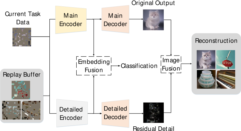
Figure 1: Our proposed bilateral MAE for efficient CIL. The Replay Buffer contains random patches selected from past task images, which is more efficient than storing whole images. Combining these with masked input data from the current task, the MAE simultaneously learns to classify and reconstruct images from the masked input. To further improve the reconstructed image quality and learned representations, embedding-level and image-level fusion is used to learn more stable representations and more detailed reconstructions for CIL.

Masked Autoencoders (MAEs) [11] were initially proposed to learn better feature representations in self-supervised learning scenarios. In this work, we see it as efficient incremental learners and propose a novel bilateral transformer architecture for efficient exemplar replay in CIL. Our main idea is simple: by randomly masking patches of input images and training models to reconstruct the masked pixels, MAEs can provide a new form of self-supervised representation learning for CIL and thus learn more generalizable representations essential for CIL. In addition, leveraging a supervised objective with classification labels benefits unsupervised MAE in training efficiency and model robustness [18]. Masked inputs can also serve as strong classification regularization by only providing a random subset of data.

When learning new tasks, the MAE can coarsely reconstruct images from sparsely sampled patches from exemplars. This process enables the framework to generate reconstructed replay data, but two problems remain: (i) the generated images tend to have less detailed and less realistic textures, which reduces data diversity for replay; and (ii) on the embedding-level, the linear classifier lacks information from low-level features. Therefore, we introduce a bilateral MAE framework with image-level and embedding-level fusion for CIL (see Fig:fig1 for a schematic overview). Fusing a complementary detailed and reconstructed image alleviates catastrophic forgetting by enriching the insufficient replay data with detailed, high-quality data distributions. Embedding-level fusion from the two branches also maintains stable and diverse embeddings, and our framework can thus achieve a better trade-off between plasticity and stability.

The main contributions of our bilateral MAE framework are threefold:

• We introduce an MAE framework for efficient incremental learning that incorporates benefits from both self-supervised reconstruction and data generation for replay.

• To further boost the quality of reconstructed images and learning efficiency, we design a novel bilateral MAE with two complementary branches for better-reconstructed images and regularized representations.

• Our approach achieves state-of-the-art performance under different CIL settings on CIFAR-100, ImageNet-Subset, and ImageNet-Full.

2 Related Work

Incremental learning.

Various methods have been proposed for incremental learning in the past few years [5, 2]. Recent works can be coarsely grouped into three categories: replay-based, regularization-based, and parameter-isolation methods. Replay-based methods mitigate the task-recency bias by replaying training samples from previous tasks. In addition to replaying samples, BiC [36], PODNet [8], and iCaRL [29] apply a distillation loss to prevent forgetting and enhance model stability. GEM [21], AGEM [3], and MER [30] exploit past-task exemplars by modifying gradients on current training samples to match old samples. Rehearsal-based methods may cause models to overfit stored samples.

Pseudo-replay methods reconstruct the old data for replay. MeRGANs [35] use conditional GANs to balance the generation of old and current samples. Besides, dreaming-relevant methods like DeepInversion [41] and AlwaysBeDreaming [33] exploit backward signals to generate images similar to the original datasets.

Regularization-based approaches, such as LwF [17], EWC [15], and DMC [44], offer methods to learn better representations while leaving enough plasticity for adaptation to new tasks. Parameter-isolation methods [24, 39] use models with different computational graphs for each task. With the help of growing models, new model branches mitigate catastrophic forgetting at the cost of more parameters and computational costs.

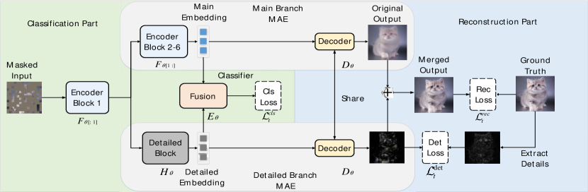
Figure 2: Overall framework of our bilateral MAE for CIL. The masked input is passed through two branches with embedding-level fusion for classification and image-level fusion for reconstruction. Full images can be generated from a small sample of input patches and the reconstructed images can be used as replay.

Self-Supervised Learning.

Self-supervised learning [7, 37, 27] has been shown to help models learn generalizable features, which makes it natural to consider its application to incremental learning. Early works used pretext tasks like patch permutation [27] or rotation prediction [10]. Contrastive learning approaches model the pairwise similarity and dissimilarity between samples [4]. By comparison, MAEs [11] learn feature representations by reconstructing images from a masked version of inputs.

There are a few works proposing self-supervision for class incremental learning. PASS [46] incorporates rotation prediction [10] to learn representations transferable across tasks. DualNet [28] uses Barlow Twins [42] to introduce a “slow” task that regularizes the “fast” incremental learning. In this paper, we explore the framework generates data for replay while applying semantic and detailed-level self-supervision, which mitigates forgetting via richer replay data and more generalizable features.

3 Continual MAE for CIL

In this section, we first define the class incremental learning problem and the basic MAE model. Then we introduce our incremental learning framework and the bilateral MAE architecture it is based on.

3.1 Preliminaries

The class incremental learning problem.

CIL aims to sequentially learn tasks with new classes while preventing or alleviating forgetting of old tasks. At a specific phase of learning task $t\in\{1,2,...,T\}$, model training can exploit only data from the current task $\{(x_{i}^{t},y_{i}^{t})\}$, where $x_{i}^{t}$ denotes image $i$ in task $t$ and $y_{i}^{t}$ its corresponding class label. A CIL model typically consists of a feature extractor $F_{\theta}$ and a common classifier $G_{\phi}$ which grows at each new task. At task $t+1$, $C_{t+1}$ new classes are added to $G_{\phi}$. The feature extractor $F_{\theta}$ first maps the input $x$ to a deep feature vector $z=F_{\theta}(x)\in\mathbb{R}^{d}$, where $d$ is the dimension of the output feature representation, and then the unified classifier $G_{\phi}(z)\in\mathbb{R}^{C_{1:t}}$ produces a probability distribution over classes $C_{1:t}$ which is used to make predictions on input $x$.

When training task $t$, the model aims to minimize losses on the current task without degrading performance on previous tasks. A common technique for mitigating forgetting is to retain a small buffer of training samples from previous tasks. Let $\epsilon$ be this buffer of previous task samples. One essential problem for CIL is the limited amount of replay data. Compared to the full data of current task $t$, only a few samples of old task classes are available (20 samples per class is a common setting), which causes imbalanced training between new and old tasks.

An MAE framework for classification.

An MAE first crops input image $x$ into non-overlapping patches, and we denote the number of patches in the full image $x$ as $N_{f}$. After patchification, the MAE randomly masks a proportion $r\in[0,1]$ of the $N_{f}$ patches, leaving only $N=\lfloor N_{f}\times(1-r)\rfloor$ patches. Then these sampled $K\times K$ pixel patches are mapped to a visual embedding of dimension $D$ using an MLP. After concatenating with a class token, the result is a tensor of size $\mathbb{R}^{(N+1)\times D}$. After positionally encoding the original patch locations, this input is passed to the MAE transformer encoder. This operation maintains the same shape of embedding. The output class token embedding can be used for classification with a cross-entropy loss $\mathcal{L}_{t}^{\mathrm{cls}}$, as shown in Fig:main.

For the MAE Decoder, learnable mask tokens are inserted into the embeddings in place of the masked patches, and the shape of output from the MAE Encoder changes from $\mathbb{R}^{(N+1)\times D}$ to $\mathbb{R}^{(N_{f}+1)\times D}$. Although the decoder is not used for classification, it helps the network back-propagate image-level reconstruction supervision to the embedding-level. This stabilizes the image embedding and helps the optimization process. Also, the reconstructed images after decoding provide richer, higher-quality replay data. To limit computation, we use a single-layer transformer block for the decoder. The additional classification loss after the encoder speeds up convergence and improves reconstruction efficiency during training. The mean squared error between the input image $x$ and reconstructed image $\hat{x}$ is used as the reconstruction loss function $\mathcal{L}_{t}^{\text{rec}}(x,\hat{x})$.

3.2 Efficient Exemplar Storage with MAEs

After training each task, we save small sample images and apply random masking. Keeping the same storage size can save more replay data per class since each sample occupies less space. For example, a masking ratio of 0.75 allows us to save 4$\times$ the number of (reconstructible) samples compared to conventional replay methods.

Let $S$ and $P$ denote the size of the image and patch, respectively. Our encoder patchifies the input image into $\frac{S}{P}\times\frac{S}{P}$ patches. We save the 2D index $(i,j)$ for each patch that is not masked. We need only one byte to save these indexes since their range is less than 255. The two additional bytes for saving this 2D index are negligible compared to the saved image patches. A masking ratio 0.75 on a 224 $\times$ 224 image requires only 36.75KB of storage. For $P=16$, the number of saved patches is $(1-0.75)\times(\frac{224}{16})^{2}=49$, and the storage of indexes is only 98B.

3.3 Bilateral MAE Fusion

To further boost reconstruction quality and embedding diversity, we propose a two-branches MAE to learn global and detailed classification and image reconstruction knowledge. We illustrate the overall framework in Fig:main. Bilateral fusion at the embedding-level aims to improve representations diversity. Reconstruction learning at the image-level yields high-quality replay data and stable self-supervision for CIL.

Mask ratio=40%	Mask ratio=75%	Difference	High-frequency
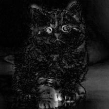
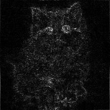
$\hat{x}_{1}$ (Eq. 9)	$\hat{x}_{2}$ (Eq. 10)	$\hat{x}_{1}-\hat{x}_{2}$ (Eq. 11)	$x^{\prime\prime}$ (Eq. 6)

Figure 3: An example of extracting detailed images with reconstructed results from different masking ratios $r_{1}$ and $r_{2}$. The third image comes from the difference between the previous two, and the last image is the extracted high-frequency component from the third image.

Embedding fusion.

In the following we use $F_{\theta[:1]}$ and $F_{\theta[1:]}$ to denote our transformer encoder’s first and following blocks. Let $H_{\theta}$ and $E_{\theta}$ represent the detailed block and embedding fusion module in Fig:main, which are standard MLP layers and attention blocks, respectively. The classification loss is computed as:

$$f = F_{\theta[:1]}(\mathrm{mask}(x,r))$$ (1)

$$z = E_{\theta}(F_{\theta[1:]}(f),H_{\theta}(f))$$ (2)

$$\mathcal{L}_{t}^{\mathrm{cls}}(x,y) = \mathcal{L}_{\mathrm{ce}}(G_{\phi}(z),y),$$ (3)

where $\mathrm{mask}(x,r)$ denotes applying random masking with ratio $r$ on image $x$, $f$ is the embedding extracted by the first encoder block, which is the input to the two branches of our Bilateral MAE, and $G_{\phi}(z)$ is the estimated class distribution used for in the cross entropy loss.

Algorithm 1 Pseudocode of our Bilateral MAE.

1:The number of task $T$, training samples $D_{t}=\{(x_{i},y_{i})\}_{t}$ of task $t$, model $\Theta^{0}$, replay buffer $\epsilon$, and masking ratios $r$, $r_{1}$, $r_{2}$.

2:model $\Theta^{T}$

3:for $t\in$ $\{1,2,...,T\}$ do

4:     $\Theta^{t}$ ← $\Theta^{t-1}$

5:     $R_{t}$ ← ReconstructOldSamples ($\epsilon_{t}$, $r$)

6:     while not converged do

7:         $(x,y)$ ← Sample ($R_{t},D_{t}$)

8:         ($\mathcal{L}_{t}^{\mathrm{cls}}$, $\mathcal{L}_{t}^{\mathrm{rec}}$) ← BilateralMAE ($x,y$)

9:         ($\hat{x}_{1},\hat{x}_{2}$) ← MaskAndReconstruct ($x$, $r_{1}$, $r_{2}$)

10:         $\mathcal{L}_{t}^{\mathrm{det}}$ ← ComputeDetailLoss $(\hat{x}_{1},\hat{x}_{2})$ 

11:         train $\Theta^{t}$ by minimizing $\mathcal{L}_{t}$ from Eq. 12

12:     end while

13:end for

Figure 4: Performance evolution over incremental tasks on CIFAR-100 on 10-, 20- and 50-task scenarios.

Method		$N$=10				$N$=20				$N$=50
		Avg $\uparrow$	Last $\uparrow$	$F\downarrow$		Avg $\uparrow$	Last $\uparrow$	$F\downarrow$		Avg $\uparrow$	Last $\uparrow$	$F\downarrow$
iCaRL [29]		65.27	50.74	31.23		61.20	43.75	32.40		56.08	36.62	36.59
UCIR [12]		58.66	43.39	35.67		58.17	40.63	37.75		56.86	37.09	38.13
BiC [36]		68.80	53.54	28.44		66.48	47.02	29.30		62.09	41.04	34.27
PODNet [8]		58.03	41.05	41.47		53.97	35.02	36.70		51.19	32.99	40.42
DER w/o P [40]		75.36	65.22	15.02		74.09	62.48	23.55		72.41	59.08	26.73
DER [40]		74.64	64.35	15.78		73.98	62.55	23.47		72.05	59.76	26.59
DyTox [9]		75.47	62.10	15.43		75.10	59.41	21.60		73.89	57.21	24.22
Ours		79.12	68.40	12.17		78.76	65.22	14.39		76.95	63.12	18.34

Table 1: Results on CIFAR-100 in average accuracy (%), last phase accuracy (%), and forgetting F (%) on 10-, 20- and 50-task scenarios.

Image fusion with detailed loss.

For the detailed head and corresponding loss, we discovered that working in the frequency domain makes it easier for the network to attend to high-frequency details, which is exactly what the detailed branch should reconstruct. We define a frequency-masking function $M(\cdot)$ that converts its argument (an image patch) to the frequency domain, then masks out low frequencies using a circular mask around the origin. As shown in Fig:main, the MAE decoder is shared by the two branches of our model since they have similar reconstruction tasks, as well as input and output shapes. Let $D_{\theta}$ be this shared decoder, then the image-level outputs of the two branches and the reconstruction loss $\mathcal{L}_{t}^{\mathrm{rec}}$ are:

$$f = F_{\theta[:1]}(\mathrm{mask}(x,r))$$ (4)

$$x^{\prime} = D_{\theta}(F_{\theta[1:]}(f))$$ (5)

$$x^{\prime\prime} = \mathrm{ifft2}(M(D_{\theta}(H_{\theta}(f))))$$ (6)

$$\hat{x} = x^{\prime}+x^{\prime\prime}$$ (7)

$$\mathcal{L}_{t}^{\mathrm{rec}} = \mathcal{L}_{\mathrm{mse}}(x,\hat{x}),$$ (8)

where $x^{\prime}$ and $x^{\prime\prime}$ are the main and residual detailed outputs, respectively, and $\mathrm{ifft2}$ is the inverse Fast Fourier Transform.

The detailed loss $\mathcal{L}_{t}^{\mathrm{det}}$ also makes use of the frequency-masking function $M$ to compare the output of the detailed branch and the difference between two MAE reconstructions of the input image:

$$\hat{x}_{1} = D_{\theta}(F_{\theta}(\mathrm{mask}(x,r_{1})))$$ (9)

$$\hat{x}_{2} = D_{\theta}(F_{\theta}(\mathrm{mask}(x,r_{2})))$$ (10)

$$\mathcal{L}_{t}^{\mathrm{det}} = ||M(D_{\theta}(H_{\theta}(f)))-M(\hat{x}_{2}-\hat{x}_{1})||_{1},$$ (11)

where $\hat{x}_{1}$ and $\hat{x}_{2}$ are two reconstructed images (detatched from the gradient computation graph) using different masking ratios $r_{1}$ and $r_{2}$, respectively. The residual difference $\hat{x}_{2}-\hat{x}_{1}$ is used as supervision in the frequency domain for the detailed branch in loss $\mathcal{L}_{t}^{\mathrm{det}}$. An illustration can be found in fig:ex.

A weighted sum of classification loss $\mathcal{L}_{t}^{\text{cls}}$, reconstruction loss $\mathcal{L}_{t}^{\text{rec}}$, and detail loss $\mathcal{L}_{t}^{\text{det}}$ is used as the overall loss for training:

$$\mathcal{L}_{t} =\lambda_{\mathrm{cls}}\mathcal{L}_{t}^{\mathrm{cls}}+\lambda_{\mathrm{rec}}\mathcal{L}_{t}^{\mathrm{rec}}+\lambda_{\mathrm{det}}\mathcal{L}_{t}^{\mathrm{det}}.$$ (12)

Pseudocode for our method is given in Algorithm 1.

4 Experimental Results

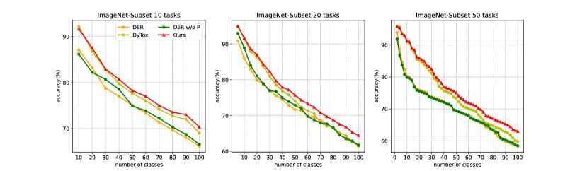
Figure 5: Performance evolution over incremental tasks on ImageNet-Subset.

Method		$N$=10				$N$=20				$N$=50
		Avg $\uparrow$	Last $\uparrow$	$F\downarrow$		Avg $\uparrow$	Last $\uparrow$	$F\downarrow$		Avg $\uparrow$	Last $\uparrow$	$F\downarrow$
BiC [36]		64.96	55.07	31.32		59.40	49.35	34.70		53.75	44.56	40.23
PODNet [8]		63.44	51.75	35.63		55.11	45.37	41.70		51.72	42.94	44.65
DER w/o P [40]		77.18	66.70	14.86		72.70	61.74	20.76		70.44	58.87	24.20
DER [40]		76.12	66.06	15.09		72.56	61.51	20.46		69.77	58.19	25.35
DyTox [9]		77.15	69.10	14.66		73.13	61.87	17.32		71.51	60.02	20.54
Ours		79.54	70.29	12.04		75.20	64.40	14.89		74.42	62.87	17.22

Table 2: Results on ImageNet-Subset in average and last phase accuracy (%) and forgetting rate F (%) on 10-, 20- and 50-task scenarios.

Method		top-1		top-5
		Avg $\uparrow$	Last $\uparrow$	Avg $\uparrow$	Last $\uparrow$
iCaRL [29]		38.40	22.70	63.70	44.00
Simple-DER		66.63	59.24	85.62	80.76
DER w/o P [40]		68.84	60.16	88.17	82.86
DER [40]		66.73	58.62	87.08	81.89
DyTox [9]		71.29	63.34	88.59	84.49
Ours		74.76	66.15	91.43	87.13

Table 3: Results on ImageNet-Full for 10 incremental tasks.

4.1 Benchmarks and Implementation

Datasets and settings.

We experiment on three datasets: CIFAR-100 [16], ImageNet-Subset, and ImageNet-Full [6] to evaluate the performance of our approach. For CIFAR-100 and ImageNet-Subset, we test on 10-, 20- and 50-task scenarios, all with equal numbers of classes per task. We evaluate the 10-task setting for ImageNet-Full in which 100 new classes are included in each task. To measure the overall accuracy after all tasks during training, we report the average accuracy of learned tasks after each task and the accuracy of all tasks at the end of incremental learning.

Implementation details.

We use the same network for all datasets. Models are trained from scratch to prevent data leakage with batch size of 1024 using Adam [14] with initial learning rate 1e-4 and cosine decay. The loss weights from Eq. 12 are set to $\lambda_{cls}=0.01$, $\lambda_{rec}=1.0$ and $\lambda_{det}=1.0$. The masking ratios are set to $r=0.75$, $r_{1}=0.75$, and $r_{2}=0.4$. Each task is trained for 400 epochs. For exemplar-based methods from the literature, we store 20 samples for each classes (as is common practice).

We use 5 transformer blocks for the encoder and 1 for the decoder. All transformer blocks have an embedding dimension of 384 and 12 self-attention heads. This design differs from the original MAE as it is much more lightweight. We save image patches occupying the same amount of memory as other methods which store 20 full images per class. For example, we select 80 images and randomly save only 25% patches from each using a masking ratio of 0.75 (thus only occupying the same space as 20 whole images). The detailed block is implemented with a 3-layer MLP keeping the dimension at 384. Further details about network architecture are given in the Supplementary Material.

4.2 Comparison with the state-of-the-art

In this section we compare our approach with the state-of-the-art, including DER [40] and DyTox [9]. In all plots and tables, “DER w/o P” denotes DER [40] without pruning, therefore leading to more parameters being added across tasks. DyTox [9] also uses a transformer architecture and we use the official codebase to reproduce its results.

CIFAR-100.

We report results in average accuracy (Avg), the accuracy after the last task (Last), and average forgetting (F) in Table 1. It is clear that under each setting our method outperforms others by a large margin. For longer task sequences, our bilateral MAE benefits from self-supervised reconstruction and richer replay data and it forgets much less compared to other methods. An overall accuracy curve is given in fig:cifar. Using the same amount of replay storage, our method outperforms DyTox by about 6% in accuracy after the last task in all three scenarios.

ImageNet-Subset and ImageNet-Full.

We report performance on ImageNet-Subset and ImageNet-Full in Tables 2 and 3, respectively. Our method outperforms DyTox [9] by 1.19%, 2.53%, and 2.85% absolute gain in accuracy after the last task on the 10-, 20- and 50-task settings, respectively. The higher average accuracy during each phase and lower forgetting also demonstrates the effectiveness of our method in alleviating forgetting. We also illustrate the performance evolution on ImageNet-Subset in fig:subset. Our method has accuracy similar to DyTox in the first task, but in later tasks our method surpasses all others, especially for long task sequences. On the larger-scale ImageNet-Full, our Bilateral MAE significantly outperforms other methods by about 3% in all metrics.

4.3 Ablation Study

Method	Replay	Reconstruction	Bilateral	Avg	Last
Baseline				73.40	62.31
Variants	✓			75.88	64.35
	✓	✓		77.48	66.54
	✓	✓	✓	79.12	68.40

Table 4: Ablative experiments on each component of our proposed method in the 10-task setting on CIFAR-100. Replay denotes using generated data from MAE for replay, Reconstruction means applying the self-supervised reconstruction loss, and Bilateral indicates introduction the detailed branch of the MAE.

$r$	Data Source	Avg	Last
0.60	Generated	77.50	67.37
0.75	Generated	79.12	68.40
0.90	Generated	77.12	67.02
N/A	Real	79.57	68.87

Table 5: Ablation on the masking ratio and quality of generated data. Experiments are on CIFAR-100 in the 10-task setting and we report top-1 accuracy in %. Data Source indicates whether replay is generated or real. In the last row we replay a selection of of real images equivalent in storage size to using $r_{1}=0.75$.

Domain	Avg	Last
Spatial	77.45	65.93
Frequency	79.12	68.40

Table 6: Ablative experiments on the detailed head. Experiments are on CIFAR-100 in the 10-task setting and we report the top-1 accuracy in %. Domain denotes to which domain our loss is applied.

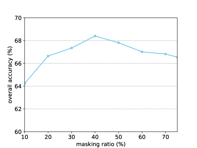
Figure 6: Ablation on masking ratio $r_{2}$ in $\mathcal{L}_{t}^{\mathrm{det}}$. The other masking ratio $r_{1}$ is set to 75% as the reference.

Ablations on different components.

Our bilateral MAE consists of a self-supervised reconstruction task, generated data for replay, and a bilateral MAE branch for image- and embedding-level fusion. We ablate on these three factors in Table 4. These three major components in our method have different functions and they cooperate to boost performance compared with the baseline by about 6%. We observe that: (a) More high-quality replay data has a direct contribution to the performance and masking ration of $r=0.75$ masking ratio yields 4$\times$ replay for the same storage cost as the baseline. (b) The reconstruction loss serves as effective self-supervision and improves performance by about 2% in average accuracy. (c) The bilateral architecture works well by improving replay data generation quality and introducing image and embedding-level supervision.

Pic 1
Pic 4
Pic 7
Pic 10
	Image	Task 1	Task 4	Task 7	Task 10

Figure 7: Reconstructions of images from ImageNet-Subset in the 10-task setting. Four original images were selected from tasks 1, 4, 6, and 10 and are shown on the left. In the remaining columns we show reconstructed images using our combined Bilateral MAE (left), only the detailed branch of our MAE (middle), and only the main branch of our MAE (right).

Masking ratio.

A key parameter of MAE [11] is the masking ratio $r$. There is trade-off on $r$: too large $r$ (e.g. 0.95) leads to poor reconstruction, which influences the quality of replay data and causes more serious forgetting. However, too small $r$ yields a limited extra amount of replay data (e.g. we can afford only about 11% extra replay data when $r$ is 0.10). The results in Table 5 show that $r=0.75$ is a good trade-off for our bilateral MAE. To verify the quality of generated data for replay, also include results using original images for replay in place of generated ones. Results in rows 2 and 4 of Table 5 show that our method achieves good quality images with less than 0.5% accuracy difference compared to replaying real images.

Frequency domain for the detailed loss.

We implemented the detailed loss by converting embeddings from the spatial domain to the frequency domain. This aims to allow concentration on high-frequency information which matches the learning objective of the detailed MAE branch. As shown in Table 6, it is beneficial to make this conversion as it leads to a more than 2% gain at the last task.

Ablation on $r_{1}$ and $r_{2}$ in the detailed loss.

We set $r_{1}$ to 0.75 for all these experiments as a reference and we vary $r_{2}$ used for computing the ground truth of the detailed loss. The trade-off on $r_{2}$ is that large $r_{2}$ results in small differences between the reconstructed results from mask ratios $r_{1}$ and $r_{2}$ and therefore there is little information in the supervisory signal for the detailed loss and the impact of the detailed branch is reduced. On the other hand, too small $r_{2}$ (e.g. 0.10) maintains most of the residual part of reconstructed images from the main branch, which may bring weak supervision for the main branch and slow its training. We show results for a range of $r_{2}$ values in fig:dms. These results show that an $r_{2}$ of about 0.40 is good for providing supervision to the detailed branch of our MAE.

Model and exemplar sizes.

To compare the effectiveness of different methods, normally models with the same or similar number of parameters are used with an equal number of exemplars. In our approach, we adapt the original MAE to be more lightweight and the number of parameters is comparable to or even smaller than DyTox, as shown in Table 7 (last row). We set the masking ratio to 75% by default and save 80 exemplars per class, and therefore the storage size for both models and exemplars is similar since our stored image patches require exactly the same as baselines using only 20 exemplars.

Method	Parameters (M)	Avg $\uparrow$	Last $\uparrow$	$F\downarrow$
DER w/o P	112.27	75.36	65.22	15.02
DyTox	10.73	75.47	62.10	15.43
Ours (MLP size = 1536)	12.89	79.12	68.40	12.17
Ours (MLP size = 768)	9.35	78.36	67.52	12.90

Table 7: Comparison of model sizes. We compare two versions of our Bilateral MAE and competing models. Experiments were conducted on CIFAR-100 with 10 tasks.

Ablation on effective buffer size.

In Table 8 we compare our method with Dytox using the same buffer size by masking input image patches in input to DyTox. All three rows use the same memory size for storing exemplars. Using 80 exemplars with masking ratio of 75%, DyTox (last row) achieves better performance than when using 20 full-image exemplars. It still performs worse than our approach, which shows that our performance gain does not simply come from the additional exemplars, but also from the integration of the MAE into our bilateral architecture with the Detailed Branch.

Reconstruction analysis.

We illustrate results of image reconstruction in the 10-task setting on ImageNet-Subset in fig:img. Randomly selected images from tasks 1, 4, 7, and 10 are shown in the left column. Our bilateral MAE learns to reconstruct images in a task-agnostic way, which helps generate reasonable results for future tasks even before learning them. The detailed branch of our MAE learns to reconstruct high-frequency details complemetary to the main branch. The results from the main branch sometimes lack sample-specific characteristics, but with the help of our proposed detailed branch the reconstructions are more accurate and provide better generated replay data.

Method	Buffer	Memory size	25% Patches	Images	Acc(%)
Ours	80	1x	✓		68.40
DyTox	20	1x		✓	62.10
DyTox$\dagger$	80	1x	✓		65.46

Table 8: Ablation on effective buffer size with equal memory usage. Dytox$\dagger$ represents applying a mask ratio $r=75\%$ directly to stored image exemplars in order to have the same number of exemplars and storage size for DyTox as in our setting.

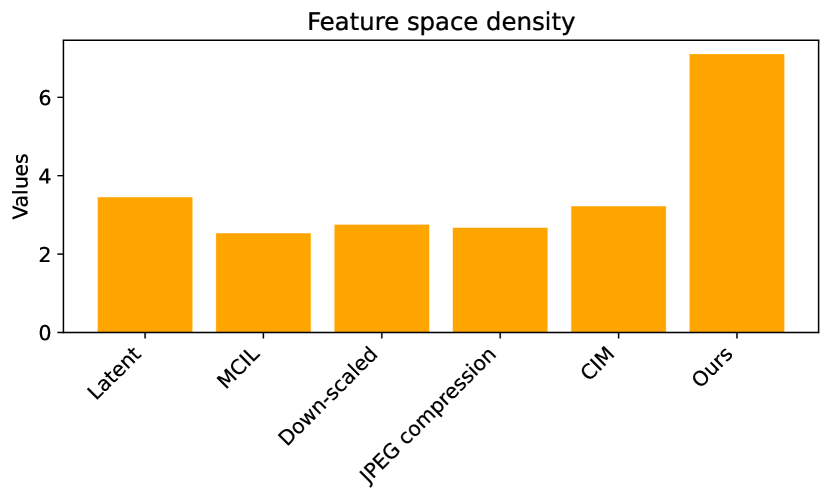
Figure 8: Comparison of feature space density $\pi$.

More generalizable representations help CIL.

We calculated the feature space density metric [32] for different methods following PASS [46]: $\pi=\pi_{intra}/\pi_{inter}$, where $\pi_{intra}$ denotes the average cosine similarity within the same class and $\pi_{inter}$ denotes the one within different classes. Increased feature space density is associated with stronger generalization under data shift [46]. We then compared feature space density after training all tasks, as shown in Figure 8 above. It is clear that Ours yields significantly higher density than other methods.

Metric	Memory	Avg$\uparrow$	Last$\uparrow$
Latent replay (CVPRW’20) [19]	-	62.44	51.30
MCIL (CVPR’20) [20]	60	63.25	53.12
Down-scaled (TNNLS’21) [45]	60	67.04	55.40
JPEG compression (ICLR’22) [34]	60	72.34	61.32
CIM (CVPR’23) [22]	60	75.30	63.05
Ours	60	79.12	68.40

Table 9: Comparison of our bilateral MAE framework with other memory-efficient methods on the CIFAR-100 10-task setting. Memory indicates the required storage space per class (in KB).

Ablation with other efficient replay methods.

We compared the replay samples generated by MAE in our framework with a variety of memory-efficient methods based on latent replay [19], synthesized exemplars [20], down-scaling [45], JPEG image compression [34], and CIM [22] (foreground extraction and background compression). All these methods use the same amount of storage (except Latent Replay uses a GAN with 4.5M parameters), while our approach achieves consistently higher performance.

5 Conclusions

In this work, we demonstrate that Masked Autoencoders are efficient incremental learners. Our approach stores random image patches as exemplars and it can reconstruct high-quality images from only partial information for replay. Furthermore, we propose a novel bilateral MAE architecture which further improves embedding diversity and reconstruction quality. Our Bilateral MAE approach significantly outperforms previous state-of-the-art methods for the same exemplar storage cost.

Acknowledgements

This work is funded by NSFC (NO. 62225604, 62206135), and the Fundamental Research Funds for the Central Universities (Nankai Universitiy, 070-63233085). Computation is supported by the Supercomputing Center of Nankai University.

References

- [1] Rahaf Aljundi, Punarjay Chakravarty, and Tinne Tuytelaars. Expert gate: Lifelong learning with a network of experts. In IEEE Conf. Comput. Vis. Pattern Recog., 2017.
- [2] Eden Belouadah, Adrian Popescu, and Ioannis Kanellos. A comprehensive study of class incremental learning algorithms for visual tasks. Neural Networks, 135:38–54, 2021.
- [3] Arslan Chaudhry, Marc’Aurelio Ranzato, Marcus Rohrbach, and Mohamed Elhoseiny. Efficient lifelong learning with a-gem. In Int. Conf. Learn. Represent., 2019.
- [4] Ting Chen, Simon Kornblith, Mohammad Norouzi, and Geoffrey Hinton. A simple framework for contrastive learning of visual representations. In International conference on machine learning, pages 1597–1607. PMLR, 2020.
- [5] Matthias Delange, Rahaf Aljundi, Marc Masana, Sarah Parisot, Xu Jia, Ales Leonardis, Greg Slabaugh, and Tinne Tuytelaars. A continual learning survey: Defying forgetting in classification tasks. TPAMI, 2021.
- [6] Jia Deng, Wei Dong, Richard Socher, Li-Jia Li, Kai Li, and Li Fei-Fei. Imagenet: A large-scale hierarchical image database. In IEEE Conf. Comput. Vis. Pattern Recog., 2009.
- [7] Carl Doersch, Abhinav Gupta, and Alexei A Efros. Unsupervised visual representation learning by context prediction. In Int. Conf. Comput. Vis., 2015.
- [8] Arthur Douillard, Matthieu Cord, Charles Ollion, Thomas Robert, and Eduardo Valle. Podnet: Pooled outputs distillation for small-tasks incremental learning. In Eur. Conf. Comput. Vis., 2020.
- [9] Arthur Douillard, Alexandre Ramé, Guillaume Couairon, and Matthieu Cord. Dytox: Transformers for continual learning with dynamic token expansion. In IEEE Conf. Comput. Vis. Pattern Recog., 2022.
- [10] Spyros Gidaris, Praveer Singh, and Nikos Komodakis. Unsupervised representation learning by predicting image rotations. In Int. Conf. Learn. Represent., 2018.
- [11] Kaiming He, Xinlei Chen, Saining Xie, Yanghao Li, Piotr Dollár, and Ross Girshick. Masked autoencoders are scalable vision learners. In IEEE Conf. Comput. Vis. Pattern Recog., 2022.
- [12] Saihui Hou, Xinyu Pan, Chen Change Loy, Zilei Wang, and Dahua Lin. Learning a unified classifier incrementally via rebalancing. In IEEE Conf. Comput. Vis. Pattern Recog., 2019.
- [13] David Isele and Akansel Cosgun. Selective experience replay for lifelong learning. In AAAI, 2018.
- [14] Diederik P Kingma and Jimmy Ba. Adam: A method for stochastic optimization. In Int. Conf. Learn. Represent., 2015.
- [15] James Kirkpatrick, Razvan Pascanu, Neil Rabinowitz, Joel Veness, Guillaume Desjardins, Andrei A Rusu, Kieran Milan, John Quan, Tiago Ramalho, Agnieszka Grabska-Barwinska, et al. Overcoming catastrophic forgetting in neural networks. Proceedings of the national academy of sciences, 2017.
- [16] Alex Krizhevsky, Geoffrey Hinton, et al. Learning multiple layers of features from tiny images, 2009.
- [17] Zhizhong Li and Derek Hoiem. Learning without forgetting. In Eur. Conf. Comput. Vis., 2016.
- [18] Feng Liang, Yangguang Li, and Diana Marculescu. Supmae: Supervised masked autoencoders are efficient vision learners. arXiv preprint arXiv:2205.14540, 2022.
- [19] Xialei Liu, Chenshen Wu, Mikel Menta, Luis Herranz, Bogdan Raducanu, Andrew D Bagdanov, Shangling Jui, and Joost van de Weijer. Generative feature replay for class-incremental learning. In IEEE Conf. Comput. Vis. Pattern Recog. Worksh., 2020.
- [20] Yaoyao Liu, Yuting Su, An-An Liu, Bernt Schiele, and Qianru Sun. Mnemonics training: Multi-class incremental learning without forgetting. In IEEE Conf. Comput. Vis. Pattern Recog., pages 12245–12254, 2020.
- [21] David Lopez-Paz and Marc’Aurelio Ranzato. Gradient episodic memory for continual learning. Adv. Neural Inform. Process. Syst., 2017.
- [22] Zilin Luo, Yaoyao Liu, Bernt Schiele, and Qianru Sun. Class-incremental exemplar compression for class-incremental learning. In IEEE Conf. Comput. Vis. Pattern Recog., pages 11371–11380, 2023.
- [23] Arun Mallya, Dillon Davis, and Svetlana Lazebnik. Piggyback: Adapting a single network to multiple tasks by learning to mask weights. In Eur. Conf. Comput. Vis., 2018.
- [24] Arun Mallya and Svetlana Lazebnik. Packnet: Adding multiple tasks to a single network by iterative pruning. In IEEE Conf. Comput. Vis. Pattern Recog., 2018.
- [25] Marc Masana, Xialei Liu, Bartłomiej Twardowski, Mikel Menta, Andrew D. Bagdanov, and Joost van de Weijer. Class-incremental learning: Survey and performance evaluation on image classification. IEEE Trans. Pattern Anal. Mach. Intell., 2022.
- [26] Michael McCloskey and Neal J Cohen. Catastrophic interference in connectionist networks: The sequential learning problem. In Psychology of learning and motivation. Elsevier, 1989.
- [27] Mehdi Noroozi and Paolo Favaro. Unsupervised learning of visual representations by solving jigsaw puzzles. In Eur. Conf. Comput. Vis., 2016.
- [28] Quang Pham, Chenghao Liu, and Steven Hoi. Dualnet: Continual learning, fast and slow. Adv. Neural Inform. Process. Syst., 2021.
- [29] Sylvestre-Alvise Rebuffi, Alexander Kolesnikov, Georg Sperl, and Christoph H Lampert. icarl: Incremental classifier and representation learning. In IEEE Conf. Comput. Vis. Pattern Recog., 2017.
- [30] Matthew Riemer, Ignacio Cases, Robert Ajemian, Miao Liu, Irina Rish, Yuhai Tu, and Gerald Tesauro. Learning to learn without forgetting by maximizing transfer and minimizing interference. In Int. Conf. Learn. Represent., 2019.
- [31] David Rolnick, Arun Ahuja, Jonathan Schwarz, Timothy Lillicrap, and Gregory Wayne. Experience replay for continual learning. Adv. Neural Inform. Process. Syst., 2019.
- [32] Karsten Roth, Timo Milbich, Samarth Sinha, Prateek Gupta, Bjorn Ommer, and Joseph Paul Cohen. Revisiting training strategies and generalization performance in deep metric learning. In Int. Mach. Learn., pages 8242–8252. PMLR, 2020.
- [33] James Smith, Yen-Chang Hsu, Jonathan Balloch, Yilin Shen, Hongxia Jin, and Zsolt Kira. Always be dreaming: A new approach for data-free class-incremental learning. In Int. Conf. Comput. Vis., 2021.
- [34] Liyuan Wang, Xingxing Zhang, Kuo Yang, Longhui Yu, Chongxuan Li, Lanqing Hong, Shifeng Zhang, Zhenguo Li, Yi Zhong, and Jun Zhu. Memory replay with data compression for continual learning. In Int. Conf. Learn. Represent., 2022.
- [35] Chenshen Wu, Luis Herranz, Xialei Liu, Joost van de Weijer, Bogdan Raducanu, et al. Memory replay gans: Learning to generate new categories without forgetting. Adv. Neural Inform. Process. Syst., 2018.
- [36] Yue Wu, Yinpeng Chen, Lijuan Wang, Yuancheng Ye, Zicheng Liu, Yandong Guo, and Yun Fu. Large scale incremental learning. In IEEE Conf. Comput. Vis. Pattern Recog., 2019.
- [37] Zhirong Wu, Yuanjun Xiong, Stella X Yu, and Dahua Lin. Unsupervised feature learning via non-parametric instance discrimination. In IEEE Conf. Comput. Vis. Pattern Recog., 2018.
- [38] Ye Xiang, Ying Fu, Pan Ji, and Hua Huang. Incremental learning using conditional adversarial networks. In Int. Conf. Comput. Vis., 2019.
- [39] Ju Xu and Zhanxing Zhu. Reinforced continual learning. Adv. Neural Inform. Process. Syst., 2018.
- [40] Shipeng Yan, Jiangwei Xie, and Xuming He. Der: Dynamically expandable representation for class incremental learning. In IEEE Conf. Comput. Vis. Pattern Recog., 2021.
- [41] Hongxu Yin, Pavlo Molchanov, Jose M Alvarez, Zhizhong Li, Arun Mallya, Derek Hoiem, Niraj K Jha, and Jan Kautz. Dreaming to distill: Data-free knowledge transfer via deepinversion. In IEEE Conf. Comput. Vis. Pattern Recog., 2020.
- [42] Jure Zbontar, Li Jing, Ishan Misra, Yann LeCun, and Stéphane Deny. Barlow twins: Self-supervised learning via redundancy reduction. In International Conference on Machine Learning, pages 12310–12320. PMLR, 2021.
- [43] Mengyao Zhai, Lei Chen, Frederick Tung, Jiawei He, Megha Nawhal, and Greg Mori. Lifelong gan: Continual learning for conditional image generation. In Int. Conf. Comput. Vis., 2019.
- [44] Junting Zhang, Jie Zhang, Shalini Ghosh, Dawei Li, Serafettin Tasci, Larry Heck, Heming Zhang, and C-C Jay Kuo. Class-incremental learning via deep model consolidation. In WACV, 2020.
- [45] Hanbin Zhao, Hui Wang, Yongjian Fu, Fei Wu, and Xi Li. Memory-efficient class-incremental learning for image classification. TNNLS, 33(10):5966–5977, 2021.
- [46] Fei Zhu, Xu-Yao Zhang, Chuang Wang, Fei Yin, and Cheng-Lin Liu. Prototype augmentation and self-supervision for incremental learning. In IEEE Conf. Comput. Vis. Pattern Recog., 2021.