Overcoming Generic Knowledge Loss with Selective Parameter Update

Abstract

Foundation models encompass an extensive knowledge base and offer remarkable transferability. However, this knowledge becomes outdated or insufficient over time. The challenge lies in continuously updating foundation models to accommodate novel information while retaining their original capabilities. Leveraging the fact that foundation models have initial knowledge on various tasks and domains, we propose a novel approach that, instead of updating all parameters equally, localizes the updates to a sparse set of parameters relevant to the task being learned. We strike a balance between efficiency and new task performance, while maintaining the transferability and generalizability of foundation models. We extensively evaluate our method on foundational vision-language models with a diverse spectrum of continual learning tasks. Our method achieves improvements on the accuracy of the newly learned tasks up to 7% while preserving the pretraining knowledge with a negligible decrease of 0.9% on a representative control set accuracy.

1 Introduction

Recent machine learning models trained on a broad dataset have shown remarkable success in both natural language processing tasks  [45] and computer vision tasks  [47, 1]. These models can directly solve a wide range of tasks, such as recognizing common objects and answering common questions, thus are dubbed as foundation models [7]. What is captured by these models covering various domains and tasks can be referred to as generic knowledge. Despite this, foundation models could still perform poorly on specific tasks. For instance,  Xiang et al. [59] found ChatGPT limited in embodied tasks, while CLIP  [47] is shown struggling in recognizing fine-grained classes like cars from different brands. Therefore, it is crucial to integrate newly revealed data with pre-trained foundation models and expand their knowledge base. As one common solution, finetuning foundation models on new data would usually result in a good performance on the new task if done carefully. This will turn the foundation model into a specific model for a specific task, as illustrated in Figure  1, and would risk losing the existing capabilities of the model or the generic knowledge it has acquired through long phases of pretraining. The effect of deteriorating the model’s previous knowledge upon new learning is a typical phenomenon of neural networks, referred to as catastrophic forgetting [40].

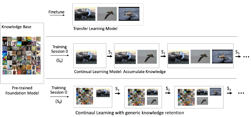
Figure 1: Different from transfer learning and conventional continual learning, we seek to continually accumulate knowledge as well as preserve the generic knowledge obtained from pre-training in the ever-going training session $\text{S}_{0}$, $\text{S}_{1}$, …

Continual learning research has been exploring the problem of accumulating knowledge without forgetting [46] over the past years and has provided valuable techniques. However, most existing works consider this process starting from a randomly initialized model  [17, 18]. Recently, with the success of large pretrained models  [51, 58], many works have considered continual learning starting from a pre-trained model [57, 56]. Nevertheless, the emphasis lies mostly on the learning and forgetting behavior of the newly acquired knowledge, in the upcoming task sequence, often side-lining the pre-trained knowledge, as illustrated in Figure  1. Generic knowledge embedded in large models provides bases for strong performance in various domains and quick transfer to different tasks; when continuously finetuning a large pretrained model on newly received tasks with no regard to preserving its pre-existing knowledge, we are losing the pre-training benefits and being left with merely a large model to deal with.

These prompt a crucial question: Can we effectively and continuously update foundation models while retaining their generic knowledge? As shown in Figure  1, an example is accommodating a generic multimodal model like CLIP [47] to specific fine-grained concepts as various types of vehicles while maintaining its generic recognition capabilities of common world concepts such as people, animals, and plants.

Towards this goal, we seek to update foundation vision-language models from a continual learning perspective while preserving their previously acquired generic knowledge. Starting from a large model pretrained on vast sources of data, it is reasonable to assume that the model has some kind of basic or related knowledge on the new upcoming data. Thus, we hypothesize that there is an implicit modularity in the foundation model and design a method to locate which parameters are most relevant to the new upcoming data. Formally, we first identify specific model layers to be updated based on model analysis works [14, 19]. Among the localized layers, we propose a mechanism to select parameters that are specialized for the task at hand. We opt for selecting parameters that small changes to their values would contribute to a greater improvement in the new task performance compared to other parameters. By doing so, we localize and update only a small number of the selected model’s parameters, while keeping a large portion of the model’s parameters untouched. In this way, we not only provide an efficient method to finetune a large pretrained model on newly arriving data but also preserve greatly the generalizability and transferability of the model. Our strategy is to be executed whenever new data corresponding to a new set of classes, a new task or domain, is received, which is the training sessions $\text{S}_{0}$, $\text{S}_{1}$, and so on in Figure  1

To facilitate a comprehensive analysis of the generic knowledge deterioration, we focus on the classification tasks and formulate the knowledge base as the zero-shot classification ability on a diverse control set containing a wide range of classes. Our main objective is to demonstrate an improvement of a pre-trained model’s performance on datasets where it initially exhibits suboptimal results, while preserving its original ability on a control set, without revisiting it. We evaluate our method on six continual learning tasks and find that by updating merely 3% of the parameters, our approach achieves performance on the new tasks superior to that achieved by methods that fully finetune the model, with almost no deterioration on the generic knowledge, only 0.97% performance loss on the control set. We further conduct comprehensive analyses to assess the impact of each component on generic knowledge forgetting.

Our contribution can be concluded as 1) We introduce the evaluation of generic knowledge forgetting in continual learning starting from foundation models. 2) To ensure the preservation of pre-trained knowledge, we propose an efficient method that localizes the learnable parameters, selects specialized parameters for the new coming data, and performs sparse updates. 3) Through comprehensive evaluations on six datasets, we demonstrate that our algorithm significantly expands the pre-trained knowledge on new tasks while still preserving the generic knowledge. Additionally, we conduct in-depth analyses to understand the impact of each component on generic knowledge forgetting.

2 Related Work

Foundation Models. Pretraining techniques have played a crucial role in establishing the so-called foundation models, such as CLIP [47], Flamingo [1], BLIP-2 [32], PaLM-E [16], and GPT-4 [45]. These models are pre-trained on vast and diverse datasets, providing them with a broad knowledge base and exceptional generalization and transferability. Consequently, many of these models can be directly applied to various tasks in a zero-shot manner. Despite their strong abilities, evaluating these foundation models remains challenging [60], given that their strengths lie predominantly in a diverse domain of generalization. While CLIP [47], an early vision-language model pre-trained on a large dataset of 400 million images and text samples, namely WebImageText, is an exception that exhibits impressive performance mainly on zero-shot classification tasks. This straightforward evaluation format allows us to thoroughly explore the changes in the model’s knowledge base when implementing updates or modifications. By studying the impact of these changes on CLIP, we aim to gain a more in-depth understanding of the potential of updating the foundation models.

Continual Learning. In the realm of continual learning, early methods [11, 29, 10, 18] train models from scratch for each specific sequence. Recent methods leverage the power of pre-trained models to handle a new sequence of tasks. Piggyback [39], as a pioneer, learns separate masks over a frozen pre-trained model for different tasks in the sequence. It requires storing the masks and access to task identification to apply the mask during inference, which is a limiting assumption. Another line of work introduces additional parameters to acquire new knowledge [56, 57, 55, 49]. Determining which set of newly added parameters to use during inference remains challenging. Additionally, the performance of such works is highly dependent on the capacity and flexibility of the added parameters, where some works only get a marginal improvement over the pretrained model [26]. Our work focuses on modifying the pre-trained models themselves, and shares some similarities with weight regularization methods [29, 2] where an importance or relevance score is estimated for the model’s parameters. A clear distinction is that the parameter importance score is estimated after learning a given task and used to prevent changing those important parameters. Differently, our approach estimates the parameter’s relevance score for a new task before starting the learning process. Our selection is to identify which parameters to update. Finally, the majority of these approaches focus on defying forgetting in the learned sequence, with no consideration for the forgetting of pre-trained knowledge. Further, they do not scale to preserving pretrained knowledge, as they either require access to the pretraining dataset [2, 29, 11] or a duplicate storage of the pretrained model [33, 4]. In contrast, we consider the accumulation of knowledge, including the pre-trained and newly acquired knowledge, without any task identification and extra storage of model weights.

Finetuning with Knowledge Preservation. It is usually observed that when finetuning foundation models on new tasks, the generic knowledge and transferability are severely deteriorated. Recently, some works [12, 41, 25, 59, 28, 62] started to tackle the issue of updating large pretrained models while preserving their transferability and the generalizability. Among them,  Meng et al. [41], Ilharco et al. [25] proposes model editing algorithms, where the models are first analyzed to pick specific layers to edit, and then algebra-based or meta-learning based methods are applied to the weight of the local layer. Usually, a local set is utilized to preserve the background knowledge. While these methods have shown promise in incorporating specific concepts into the model, their impact on the generic knowledge remains uncertain, as discussed by  Onoe et al. [44]. Additionally, most of these techniques are designed for specific models for small-scale sample-wise edit of concrete mistakes and updates. Moreover, they are centered around language models, where the input data has a stronger relationship to the concept being edited, leaving the vision models, where the input images can contain various of unrelated visual concepts, relatively unexplored. In contrast, we are interested in allowing continuous model updates on a set of new coming data samples, which can be scaled up to a larger number of concepts and a longer never-ending sequence.

Additionally,  Xiang et al. [59] proposed to finetune language models for embodied tasks while maintaining their generalization ability to handle unseen embodied tasks. They suggested fine-tuning language models with LoRa [24], i.e., low rank updates, to ensure compute efficiency, while applying EWC regularization [29] to reduce forgetting of the pretrained knowledge. On the multimodal models end,  Zheng et al. [62] considered to prevent zero-shot transfer degradation in the continual learning of CLIP by performing distillation on the pre-trained model weights. However, it requires access to a massive dataset to represent the pre-training distribution, which is not a trivial assumption and far from being computationally efficient. In this work, we aim to update foundation models, such as CLIP, continually to recognize additional concepts and preserve their transferability, while striving for efficiency.

3 Continual Learning From Pretrained Models

In Class Incremental Learning (CIL), we are given a dataset $D^{t}_{\text{train}}=\{x_{k},y_{k}\}_{k=1}^{N_{t}}\sim\mathcal{D}^{t}$ sampled from a task-specific distribution $\mathcal{D}^{t}$ for each task $t\in\{1,\ldots,T\}$ sequentially, where $X^{t}_{\text{train}}=\{x_{k}\}_{k=1}^{N_{t}}$ is a set of images and $Y^{t}_{\text{train}}=\{y_{k}\}_{k=1}^{N_{t}}$ is the set of the corresponding labels with $y_{k}\in Y^{t}_{\text{train}}$. Here $Y^{t}_{\text{train}}$ is the label space of task $t$. Note that while we focus on image-based data, our method can be extended to any modality. We are given a model parameterized by $\theta$ pre-trained on a vast pre-training dataset $D_{p}\sim\mathcal{D}_{p}$ sampled from the pre-training distribution, which is inaccessible during the CIL procedure. During the learning of each task, the model parameters $\theta$ are to be optimized to minimize a loss function $\mathcal{L}$ on the current training set $D^{t}_{\text{train}}$. The loss function depends on the task at hand and the model deployed. For CLIP model [47] and image text pairs data, we deploy the same contrastive loss used for CLIP pretraining. After the learning of each task, we evaluate our model on both the validation set of the seen distributions of the CIL sequence $D_{\text{test}}^{1:t}$, where $D_{\text{test}}^{t}\sim\mathcal{D}^{t}$, and a small control set $D_{\text{control}}\sim\mathcal{D}_{p}$ sampled from the pre-training distribution.

4 Selective Parameter Update

Most existing continual learning methods that start from randomly initialized models optimize all parameters equally, as such a starting point has no knowledge or relevance to the task being learned. However, foundation models often have a reasonable initial performance on novel tasks, indicating some pre-existing knowledge relevant to these tasks. With the strive for efficiency and the preservation of the generic knowledge, we suggest identifying a small set of parameters corresponding to tasks in hand and only updating them instead of modifying all the pre-trained model parameters. We now introduce how to localize the update to specific layers and how to identify a sparse set of specialized parameters to be optimized.

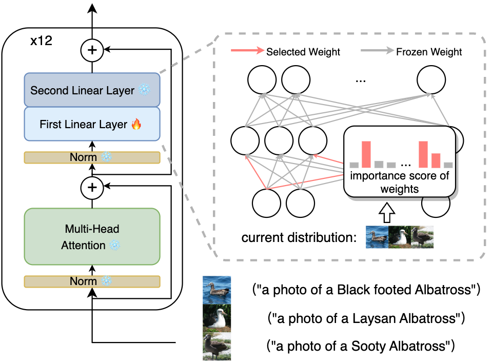
Figure 2: We first localize our update to the first layer of MLP blocks, and then select a sparse set of parameters specialized to the new task to update.

Localization. The objective of our work is to accumulate new knowledge without catastrophically forgetting the generic knowledge. To achieve this, we introduce a method that performs local changes restricted to specific layers in the pre-trained transformer backbones. As shown in Figure 2, a transformer block contains a multi-head attention block and a two-layer MLP block. Recent research on transformer analysis [19] has shown that MLP blocks emulate key-value neural memories, where the first layer of MLP acts as memory keys, operating as pattern detectors. Each individual key corresponds to a specific pattern seen in the input data. Whereas, the second layer learns the distribution over the detected patterns. Later,  Meng et al. [41] adopted casual tracking to analyze the contribution of attention layers and MLP layers to the output prediction. It performs comparisons by computing the average effects of restoring activations at these locations over a corrupted input. A large body of model editing work  [41, 22, 43, 42] follows these analyses and edits MLP layers to achieve local modification of facts.

Our work aims to add, update, or refine current knowledge embedded in the model, and with the analogy to the key-value memories, we opt for refining the keys (corresponding to pattern detectors) to accommodate the new information. Empirically, we investigated whether we need to change the patterns’ distributions represented by the second MLP layer and attention layer as well, and it turned out that updating the first layer is sufficient and more effective, as we shall show in the experiments Section 5.3. With this in mind, we localize the model updates to the first layer of the MLP in each transformer block. With such localization, our candidate parameters to change are only around one third of the total parameters. To further verify our choice, we follow the casual analysis proposed by Meng et al. [41] in Supplementand show that the changes on the first MLP layer, that we localize the update to, have a larger effect on the model predictions than changes in attention layers; which support our localization strategy.

Parameter Selection. Pre-trained foundational models have inherent knowledge, as evidenced by their capacity to execute diverse tasks without fine-tuning. Moreover, recent investigations [19, 20, 6] have unveiled the correlation between the concepts and specific neurons’ output in foundation language models. Therefore, we hypothesize that there exists some sort of modulation and specialization among specific neurons and their corresponding parameters in foundation models. Updating the most related neurons while keeping other neurons unchanged will not only facilitate the learning of new tasks but prevent the inference between different concepts in the new task sequence and between newly learned concepts and ones learned from pre-training.

Upon these, we propose to identify which parameters in the first MLP layer are specialized on the task at hand based on a scoring function. As shown in Figure  2, we select parameters associated with top scores and minimize the new task loss by only updating those selected parameters. In practice, we only make small changes to 3% of the total parameters, leading to efficiency and effectiveness in preventing forgetting, as we shall show in later experiments. We now formally outline our parameter selection methodology.

We receive the current task dataset $D^{t}$ representing a task $t$ in a continual learning sequence and localize the updates to the first MLP layer $\theta^{l}$ for each transformer block, where $l$ denotes the localized first layer indexed over transformer blocks. We aim to define an element-wise scoring function $\mathcal{S}(\theta^{l}_{i,j},D^{t})$, for each parameter in a localized layer $\theta^{l}_{i,j}$; $i,j$ refers to the parameter connecting an input element $i$ (the $i$-th output entry of the attention layer) to the neuron $j$ in the first MLP layer. We propose to select a subset of parameters $\theta_{U}^{l}\subseteq\theta^{l}$ that has the largest scores $\{\mathcal{S}(\theta^{l}_{i,j},D^{t})\}$, subject to $\frac{|\theta^{l}_{U}|}{|\theta^{l}|}=r$, where $|\cdot|$ is the parameter size and $r$ is the selection rate. This set is then expected to combine the most relevant parameters to the current task represented by the dataset $D^{t}$. We select parameters regardless of their corresponding neurons and ablate the effect of selecting the entire parameters of identified neurons in Supplement. In the sequel, we present our parameter scoring function. For clarity, the presentation of the method is focused on $\theta^{l}$, and it can be generalized to a plural of selected layers covering all transformer blocks.

Gradient-Based Scoring Function. We aim to identify which parameters are more relevant to the new task at hand. We formulate this as finding parameters where small changes to their values could lead to a greater improvement in the task performance, with the loss function as a proxy. When achieving this, we only make small changes to the model and thus can preserve the generic knowledge while improving the new task performance. Specifically, we can approximate the change in the loss function upon small changes $\delta$ in the parameters’ values with

$$\small\mathcal{L}(\theta^{l}+\delta;x_{k})-\mathcal{L}(\theta^{l};x_{k})\approx\sum_{i,j}g_{ij}(x_{k})\delta_{ij},$$ (1)

where $\mathcal{L}$ is the loss function, $g_{ij}(x_{k})=\frac{\partial(\mathcal{L}(\theta^{l};x_{k}))}{\partial\theta^{l}_{ij}}$ is the gradient of the loss function regarding the parameter $\theta^{l}_{ij}$ evaluated at the data point $x_{k}\in D^{t}$, and $\delta_{ij}$ is the local change in parameter space. The above first-order approximation suggests that a fixed small changes made to parameters with the larger gradient magnitude $\parallel g_{ij}\parallel$ in the opposite direction of the gradient would incur a larger reduction in the loss function, and hence greater improvements with minor changes.

Following this, we define our scoring function as:

$$\small\mathcal{S}(\theta^{l}_{ij},D^{t})=\|\frac{1}{N^{\prime}_{t}}\sum_{k=1}^{N^{\prime}_{t}}g_{ij}(x_{k})\|,$$ (2)

where $N^{\prime}_{t}$ is the number of samples we use to compute the gradient. Note that $N^{\prime}_{t}$ can be much smaller than the total number of samples in the dataset, $N_{t}$ as we shall show in the Supplement.

Sparse update. Upon selecting the relevant parameters $\theta_{U}=\{\theta^{l}_{U}\}$, we freeze all other model parameters and learn the current dataset $D^{t}$ by only optimizing $\theta_{U}$.

Following the current practice in class incremental learning methods, [4, 18, 57] we deploy a replay buffer to reduce the forgetting across the new tasks sequence. We keep a replay buffer $\mathcal{M}$ of a fixed size, and sample batches from it of the same size as the batch from the current dataset at each optimization step. We update the replay buffer at the end of learning of each task by experience replay [11].

Our final objective function at task $t$ can be written as

$$\min_{\theta_{U}}\mathcal{L}(\theta;D^{t}_{\text{train}})+\mathcal{L}(\theta;\mathcal{M})$$ (3)

where $\mathcal{L}(\theta;D)$ is the current task loss computed on the training set $D^{t}$.

Algorithm applicability. Our algorithm involves three key steps: localizing update layers, selecting relevant parameters, and training on the new task with sparse updates. It is important to note that while we primarily delve into the localization within the transformer architecture, the concept of selectively updating certain layers while keeping others frozen to achieve efficiency and comparable performance is not confined to this architecture alone.  [48, 8]. Should the need arises to extend our approach to different architectures, the first step of our methodology can be readily adapted. Furthermore, the processes of parameter selection and sparse updates remain architecture-agnostic, making them versatile across various model structures. We refer to our method as SPU , short for Selective Parameter Update.

	Aircraft			Birdsnap			Cars			CIFAR100			CUB			GTSRB			Average
	Acc.	F.	C.	Acc.	F.	C.	Acc.	F.	C.	Acc.	F.	C.	Acc.	F.	C.	Acc.	F.	C.	Acc. In.	Avg. F.	C. Drop
Frozen [47]	24.45	-	63.55	43.20	-	63.55	64.63	-	63.55	68.25	-	63.55	55.13	-	63.55	43.38	-	63.55	0.0	-	0.0
FLYP [21]	18.63	39.93	41.04	44.06	23.43	51.06	51.64	25.65	52.25	46.26	37.78	26.53	45.74	26.62	44.30	21.76	55.48	1.59	-11.82	34.81	27.42
+ MAS [2]	33.69	27.50	61.09	47.42	17.12	60.05	69.43	9.18	61.17	63.88	21.16	49.35	61.72	12.05	57.35	42.04	25.38	42.06	3.19	18.73	8.37
+ ER [11]	41.42	31.48	50.41	56.22	21.63	56.72	69.08	16.42	58.07	82.86	3.41	42.10	64.07	17.72	51.30	96.28	-7.40	17.34	18.48	13.88	17.56
+ ER + LwF [33]	36.08	18.12	63.06	50.23	10.20	62.08	72.56	4.04	62.59	74.32	8.16	55.71	65.11	5.90	62.05	53.56	11.86	57.99	8.80	9.71	2.97
+ ER + PRD [4]	37.11	17.35	63.38	51.34	9.45	62.85	74.08	3.75	62.96	79.66	3.10	59.01	65.92	6.55	62.09	63.00	12.44	61.04	12.01	8.77	1.66
LoRA-EWC  [59]	30.36	12.23	62.82	45.91	12.12	62.53	66.11	3.89	61.39	67.35	15.28	55.27	58.72	4.92	61.27	46.14	13.23	61.70	2.59	10.28	2.72
+ ER (r=8)	33.12	12.14	62.99	50.28	8.70	62.74	70.51	0.88	62.49	81.27	-0.70	59.90	62.36	2.99	62.80	89.87	-7.17	61.62	14.73	2.81	1.46
+ ER (r=96)	33.75	11.75	62.91	50.52	8.96	63.00	71.17	0.46	62.39	82.10	-1.59	59.91	62.31	2.81	62.72	90.01	-7.46	61.66	15.14	2.49	1.45
L2P [57]	32.20	21.73	43.43	24.37	36.17	44.63	67.04	11.22	42.53	67.71	18.81	39.61	64.04	6.82	45.51	75.45	2.68	34.05	5.29	16.24	21.92
DualPrompt [56]	26.61	17.20	56.31	36.34	30.23	46.43	63.30	18.67	55.76	61.72	19.87	42.37	64.38	12.94	55.63	69.65	8.43	40.37	3.83	17.89	14.07
SLCA [61]	29.40	11.45	63.49	43.18	9.28	63.33	62.65	4.42	63.29	70.03	0.19	60.23	53.87	7.75	63.31	46.01	0.83	62.76	1.02	5.65	0.81
ZSCL [62]	30.96	15.65	65.53	49.85	13.28	63.13	67.79	8.27	62.90	80.50	1.05	61.90	61.09	7.69	62.78	62.92	13.54	62.92	9.01	9.91	0.36
SPU - Ours	44.43	14.42	63.48	55.35	12.78	61.94	77.51	3.26	63.42	83.99	-0.39	61.38	71.51	4.84	62.87	94.25	-7.87	62.55	21.34	4.51	0.94

Table 1: Average Accuracy (Acc.), Forgetting (F.), and control set Accuracy (C.) of our method SPU and baselines on 6 CIL sequences, demonstrating our superior knowledge accumulation and preservation. We highlight parameter efficiency via parameters size and learnable parameters rate, and data efficiency via data use.

5 Experiments

We evaluate our proposed framework on various datasets compared to different methods and baselines in Section 5.2, and analyze different components of our method and ablate our design choices in Section 5.3. We provide further ablations on defying generic knowledge loss in the Supplement.

5.1 Setup

Backbone. We assess the efficacy of our approach through its application to vision-language classification tasks, given the relatively robust measurement of the knowledge base in such tasks. We choose the pre-trained CLIP-ViT/B-16 [47] as our backbone.

Datasets. We evaluate the performance of our algorithms on a total of six datasets— four fine-grained datasets (Birdsnap [5], CUB-200-2011 [53], FGVC-Aircraft [38], Stanford Cars [30]), one coarse dataset (CIFAR100 [31]), and one out-of-distribution dataset (GTSRB [50]). These datasets are chosen primarily based on their initially low zero-shot performance with CLIP pre-trained models. To form the continual learning sequences, we split each dataset into 10 subsets with disjoint classes composing 10 tasks. For methods that leverage a replay buffer, we use a buffer size of around 4% of the dataset size. Ablation study of buffer size is shown in Section 5.3. For more comprehensive information, including detailed statistics, data sources, and implementation details, please refer to the Supplement.

Baselines. We conduct a comprehensive comparison of our method against various baselines. Firstly, we evaluate our approach against the best fine-tuning method of CLIP, FLYP  [21]. We further integrate with FLYP classical continual learning components to evaluate their performance on the CLIP backbone, including ER [11], weight regularization method, MAS [2], and functional regularization methods LwF [33] and PRD  [4]. We combine these functional regularization methods with a replay buffer. We further consider the latest pre-trained model based continual learning techniques. L2P [57], DualPrompt [56], and SLCA  [61]. Finally, we compare to two recent methods that target knowledge retention of foundation models. ZSCL [62] designed for CLIP [47] and LoRA-EWC [59] which combines LoRA [24] and EWC [29] to finetune an LLM, here we adapt it to CLIP. Results, evaluation with ImageNet pretrained backbones of these methods, and discussion are in the Supplement.

Evaluation Metrics. We measure the Acc. at the end of the class-incremental process, as well as the forgetting rate following prior arts [11, 10]. Additionally, we aim to understand how the knowledge base shifts as we continually update the pre-trained models. To achieve this, and similar to [25], we evaluate a continually trained model $M$ on a diverse dataset representing generic knowledge, i.e., the validation set of ImageNet [15], which acts as a control set (C.). We report the zero-shot classification accuracy on (C.), and compare it with that from the frozen pre-trained models.

To provide a comprehensive view of model performance across all $N_{D}$ datasets $\{D_{i}\}_{i=1}^{N_{D}}$, we denoted the model parameters trained after $D_{i}$ as $M_{i}$, and frozen model performance on $D_{i}$ as $M_{\text{f}_{i}}$. We present the increment of Average Accuracy (Acc. In.) across these datasets as

$$\footnotesize\text{Acc. In.}(M)=\frac{1}{N_{D}}\sum_{i=1}^{N_{D}}\text{Acc.}(M_{i})-\text{Acc.}(M_{\text{f}_{i}}),$$ (4)

the average forgetting rate (Avg. F.)

$$\footnotesize\text{Avg. F}(M)=\frac{1}{N_{D}}\sum_{i=1}^{N_{D}}\text{F. }(M_{i}),$$ (5)

and the average drop of control set accuracy (C. Drop).

$$\footnotesize\text{C. Drop}(M)=\frac{1}{N_{D}}\sum_{i=1}^{N_{D}}\text{C.}(M_{\text{f}})-\text{C.}(M_{i}),$$ (6)

Implementation Details. We follow  [21] to both perform selection and sparse update on the visual tower and text tower of the CLIP model, and use contrastive loss as our loss function. Within our algorithm, we use a selection rate of 10%, which optimally balances learning and forgetting. We perform an ablation study on the selection rate in section  5.3. More implementation details of all baselines can be found in the Supplement.

5.2 Results

We present the comparison between our approach and other methods in Table 1. In the subsequent sections, we delve into our observations from the dual lenses of learning and forgetting.

Comparison with other methods. In our experiment, we view accumulating novel knowledge as prioritized, at the same time also pay attention to knowledge retention. Regrading the accuracy of newly learned knowledge (Acc.), we achieve state-of-the-art results in four out of six datasets, i.e., Aircraft, Cars, CIFAR100, and CUB, and comparable results in Birdsnap and GTSRB, with a notable average margin of 2.86% over the existing continual learning methods. We analyze how our scoring function contribute to the achievement in Section  5.3.

Regarding the knowledge retention, our approach achieves control set accuracy drop (C. Drop) of 0.94% which is the least drop among methods with no external data access, and is comparable to that of ZSCL, which requires access to the additional Conceptual Caption dataset for knowledge retention. This brings efficiency concerns, which we will elaborate later in Section  5.4. In spite of ZSCL preservation of the generic knowledge, this comes at the expense of the new tasks increment average accuracy which is  12% lower than ours.

The superior results in new task accuracy and control set accuracy demonstrates that SPU can effectively extends the knowledge base during continual learning.

Among the continual learning methods we have compared with, FLYP+ER stands as the only comparable contender in terms of average accuracy of new task. This mainly benefits from the balanced loss terms on buffer data and current task data. However, it exhibits a significant drawback in the form of forgetting, averaging at 13.88% in the forgetting of the current dataset, and a notable decrease of 17.56% in average control set accuracy.

Notably, distillation-based methods such as FLYP+ER+LwF/PRD and ZSCL generally perform good at preserving the pre-trained knowledge, all displaying control set accuracy drop of less than 3%. These line of algorithms impose penalty of the model output change by comparing the outputs from the newly finetuned model and a pre-trained model. However, their flexibility in learning the new tasks, as indicated by their average accuracy, remains limited, reflecting a discernible gap of over 8% when compared to our method. While SLCA achieves the second best results of 0.81% in preserving the pre-trained knowledge, but it almost cannot improve the new task when compared to SPU .

LoRA based methods exhibit extraordinary performance in eliminating forgetting. In the forgetting of the new tasks, LoRA-EWC combined with ER can achieve only 2.49% of forgetting. In the preservation of pre-trained knowledge, LoRA-EWC has only 1% - 3% control set accuracy drop depending on the rank choice and buffer choice. However, this is a larger drop than our marginal 0.94% drop in control set accuracy. In spite of their knowledge retention ability being slightly worse than ours, their average increment accuracy on new tasks is lower than ours, with at least a margin of 6.2%.

	Aircraft			Birdsnap			Cars			CIFAR100			CUB			GTSRB			Average
	Acc.	F.	C.	Acc.	F.	C.	Acc.	F.	C.	Acc.	C.	H.	Acc.	C.	H.	Acc.	F.	C.	Acc. In.	Avg. F.	D. Drop
Attention layers	41.34	14.68	64.02	55.22	11.73	62.53	76.35	3.61	63.73	84.00	-0.35	62.49	70.99	4.03	63.39	92.41	-8.23	63.20	20.21	4.24	0.32
First MLP layers	44.43	14.42	63.48	55.35	12.78	61.94	77.51	3.26	63.42	83.99	-0.39	61.38	71.51	4.84	62.87	94.25	-7.87	62.55	21.34	4.51	0.94
Second MLP layers	43.32	14.02	63.24	54.98	12.25	61.17	76.91	3.24	62.77	83.59	-0.42	59.57	70.00	5.40	62.19	93.32	-8.38	61.24	20.51	4.35	1.85
Both MLP layers	44.21	14.78	63.32	55.10	13.46	61.32	77.25	3.79	63.13	84.15	-0.31	60.47	71.23	5.42	62.34	94.18	-7.85	61.65	21.18	4.88	1.51

Table 2: Compared to various choice of selected layers, our choice (in gray background) achieves the best performance in new task accuracy (Acc.) while has comparable results in control set accuracy (C.)

	Aircraft			Birdsnap			Cars			CIFAR100			CUB			GTSRB			Average
	Acc.	F.	H.	Acc.	F.	H.	Acc.	F.	H.	Acc.	F.	H.	Acc.	F.	H.	Acc.	F.	H.	Acc. In.	Avg. F.	C. Drop
Random	38.34	11.19	63.83	54.74	8.92	63.64	74.62	2.91	63.64	83.84	-2.17	62.88	67.36	3.59	63.77	86.51	-6.06	63.30	17.73	3.06	0.04
SPU	44.43	14.42	63.48	55.35	12.78	61.94	77.51	3.26	63.42	83.99	-0.39	61.38	71.51	4.84	62.87	94.25	-7.87	62.55	21.34	4.51	0.94
piggyback [39]	43.68	14.86	63.66	53.81	13.97	61.91	76.58	3.94	63.45	83.93	-0.70	61.45	70.97	5.00	62.98	93.02	-7.83	62.30	20.49	4.87	0.92
Mask	43.95	14.80	63.58	54.23	13.10	62.23	76.92	3.56	63.43	84.30	-1.07	62.08	71.11	4.78	62.98	92.41	-7.33	62.63	20.65	4.64	0.73

Table 3: Compared to random selection, our superior performance (in gray background) implies the selected weights specialized to the task. Compared to training-based scoring functions, our training-free function performs better in new task accuracy and control set accuracy.

Fine-grained Datasets. The diverse characteristics of various datasets also lead to distinct behaviors. Across fine-grained datasets like Aircraft, Cars, and CUB, we achieve SOTA average accuracy, outperforming the baselines by around 3%, while demonstrating minimal degradation in control set accuracy of less than 1%.

Out of Distribution Dataset. We view GSTRB as out of distribution for CLIP pretraining, as it is the only considered dataset where the zero shot performance of CLIP is significantly lower than the performance of a linear classifier trained on ResNet50 features [47]. Its extremely detailed class descriptions (such as “blue circle with white forward arrow mandatory”) make the deep semantic understanding of images, such as the exact meaning of the signs, less important. In these experiments, GSTRB proves an outlier for SOTA CIL methods with significantly low Acc., while our method proves robust. FLYP+ER achieves an average accuracy of 96.28% in GTSRB, but at the expense of a 17.34% control set accuracy, equating to around 60% accuracy loss, indicating a large decay in the generic knowledge after learning such out of distribution datasets. In contrast, our proposed method achieves competitive accuracy, concurrently delivering small control set loss of around 1%, signifying minimal loss of generic knowledge.

Coarse Dataset. In contrast, in the case of the coarser CIFAR100 dataset, we still achieve an impressive SOTA learning accuracy of 83.99%, albeit with a marginal trade-off of approximately 2% in control set accuracy. Even with this reduction, SPU stands out as significant compared to most other continual learning techniques that experience losses of generic knowledge ranging from 4% to 21%. This phenomenon can be attributed to that CIFAR100 encapsulates a degree of generic knowledge, possibly causing interference in the information on control sets like ImageNet.

5.3 Ablation Study

In this section, we perform ablation studies on the individual components comprising our algorithm to validate the rationale behind our design of these components. Refer to the Supplementfor more details and full results.

Which layer to update? We compare localizing the update to the first MLP layer parameters (our choice) to that of the second MLP layers and both MLP layers together. We also consider the choice of Attention layers. In the experiment of Attention layers and second MLP layers, we updated 10% of parameters as what we do in our choice. In the experiment of updating both MLP layers, we updated 5% parameters of each layer to match the selection rate. Results reported in Table 2. Updating the Attention layers helps to migrate the forgetting better, which is consistent with the LoRA-EWC performance. However, it has obvious worse performances on the new tasks accuracy in Aircraft, Cars, CUB, and GTSRB. Updating parameters from the second layer suffers double the generic knowledge loss compared to that of the first layer parameters. Updating parameters in both layers is also worse in both forgetting and control set accuracy than localizing the updates to the first layer only. We conclude that localizing the updates to selected parameters of the first layer only is sufficient to achieve the best trade-offs.

Do the selected weights represent the task? We want to validate whether the selected parameters by our scoring function can represent the task at hand in Table 3. We first compare our scoring function with a random scoring function. The results indicate that with sparse update, we can preserve the knowledge learned from pre-training. However, the Avg. In. of the random select baseline, 17.73%, is worse than the Avg. In. of FLYP+ER, 18.48%. This suggests that with only sparse update we may miss some important representations to the new task in the parameter space. However, with our scoring function, we do not only improve over random select, but over full finetune (FLYP+ER) in continual learning by mitigating forgetting. This implies that our selected parameters are specialized in the current task concepts, thus changing them will cause the least interference with other tasks.

There are also existing methods, e.g. Piggyback [39], that train a mask for parameter selection. We note that these methods require an additional phase of training; thus SPU is more computationally efficient. Furthermore, in Table 3, we compare SPU with Piggyback and a learnable variant of our scoring function, denoted as Mask. Details of the implementation can be found in Supplement. Comparing with these two methods, our gradient-based scoring function is better in both new task learning (Acc.) and in knowledge preservation (C.).

Selection Rate	Acc. In.	Avg. F.	C. Drop
0.01	17.70	3.10	1.11
0.10	21.34	4.51	0.94
0.50	21.73	7.76	0.95

Table 4: Ablation on selection rate of SPU. Our approach achieves the best trade-off when selecting 10% weights.

Selection rate. Table  4 illustrates the variants of our method under varying selection rates applied to the first layer of MLP blocks. Across all selection rates, SPU demonstrates competitive average accuracy, forgetting, and control set accuracy when compared with other baselines in Table  1. Even with a 0.5 selection rate, the learnable parameters comprise only 30% of the total parameters. We note that as the selection rate increases, there is a marginal enhancement in learning performance, but accompanied by a compromise in forgetting. For instance, raising from 0.1 to 0.5 selection rate, the Average Accuracy improves around 0.5% but the forgetting also raises around 3%. Therefore, we opt for a selection rate of 0.1, which gives the best trade-off between the accumulation of the new knowledge and the preservation of the pre-trained knowledge.

Buffer Size / Total Size	FLYP+ER			SPU
	ACC. In	Avg. F.	C. Drop	ACC. In	Avg. F.	C. Drop
1%	8.97	22.27	19.18	16.18	10.28	1.00
2%	13.24	19.35	18.24	18.63	8.14	0.96
4%	18.48	13.88	17.56	21.34	4.51	0.94

Table 5: Ablation on buffer size and comparison to FLYP+ER. Our approach has lower performance drop and small forgetting when the buffer size decreases

Buffer size. In Table  1, we present the outcomes of SPU using a buffer size equivalent to 4% of the total dataset size. Table  5 shows our performance over an array of buffer sizes, ranging from 1% to 4% of the total dataset size, compared with ER. Evidently, our algorithm excels in preserving pre-training knowledge across all buffer sizes, all with less than 1% drop in control set accuracy. As we decrease the buffer size, FLYP+ER encounters substantial influence; our method with 1% buffer size doubles Avg. Acc. improvement of FLYP+ER with 1% buffer and suffers 50% less forgetting with merely 1% control set accuracy loss.

5.4 Efficiency

Method	Full Parameter	Trainable Parameter	Extra Data Source
FLYP	149.5M	149.5M (100%)	-
LoRA-EWC (r=96)	154M	5.90M (3.79%)	CC12m
ZSCL	299M	149.5M (50%)	CC12m
SPU (ours)	149.5M	4.72M (3.15%)	-

Table 6: Parameter efficiency and data efficiency of various CL algorithms. Our approach is parameter and data efficient in updating a small portion of parameters with no added parameters and no requirement of extra data source.

We consider efficiency from two perspectives, parameter efficiency and data efficiency, as shown in Table  6. For parameter efficiency, we follow  [24, 23, 27] to report the full parameter size and trainable parameter size. While most of the current methods necessitate a complete parameter update, SPU only requires an update of a sparse subset of parameters, which only consists of 2.7% of the total model’s parameters. Besides this, we neither require adding extra parameters to the model as in LoRA-EWC and L2P, nor storing the frozen pre-trained model as in ZSCL. Using the pre-trained model consumes extra GPU memory during the training. Adding extra model parameters consumes extra GPU memory during the training, and disk memory when saving the model. This influence may be ignorable in a limited number of tasks. However, continual learning expects an ever-going algorithm. Then the storage problem becomes profound, together with the added model components (prompt, adapter, and so on) choosing problem, as in L2P.

For data efficiency, our algorithm does not require extra data source, making it light to deploy on various applications without loading huge datasets. LoRA-EWC and ZSCL are the only two methods achieving similar control set accuracy to SPU . However, LoRA-EWC takes Conceptional Caption 12M (CC12M)  [9] to compute the Fisher information of pre-trained task, and ZSCL uses CC12M for distillation.

We further perform an ablation study on the number of samples $N_{t}^{\prime}$ used to approximate the scoring function. Results show that our method can still have good performance even when using only one batch of samples for the approximation. This implies that the computation of the scoring function is also efficient which does not require a full pass of the data prior to the training, and can be done transparently with the first received batch. Details are in Supplement.

6 Discussion

With the rise of advanced foundation models pretrained on vast datasets, we propose a method that preserves pre-learned information in continual learning. We base on the fact that foundation models already have initial knowledge for the task in hand, and identify specific model layers and parameters corresponding to this knowledge for sparse updates. As such, we perform small update for the model to cope with the new knowledge while preserving the previously acquired generic knowledge. We evaluate our method extensively and show superior performance. However, our current method operates unidirectional, and future research could explore knowledge accumulation across diverse domains. Additionally, expanding our focus from discriminative to generative tasks would enhance the applicability of our techniques.

Appendix A Casual Tracking for Localization

In this paper, the weight selection is localized to the first MLP layer within transformer blocks. We discussed such localization in prior model editing and probing works in Section 4. We further perform casual tracking to validate the localization.

Vig et al. [52] quantifies the contribution of intermediate variables in causal graphs for causal mediation analysis. Based on this, Meng et al. [41] proposed casual tracking for identifying neuron activations that are decisive in a language model’s factual predictions. Casual tracking identifies specific locations that contribute to the input’s recognition by computing the average effects of restoring activations at these locations on a corrupted input. We adapt the casual tracking to CLIP models and formulate the computation of average indirect effect (AIE) in the following.

In CLIP model with ViT backbone, we freeze one tower of visual or text and perform casual tracking on the other. Take the casual tracking on image tower for example, we do the next three runs:

• Clean run. We pass an image-text pair into the model and store activations of the visual tower $\{a_{i}^{\ell}|i\in[1,T],\ell\in[1,L]\}$, and get the similarity score $S$. Here $T$ is the number of tokens, and $L$ is the number of layers.

• Corrupted run. We then pass the image into visual tower by adding noises to the image embeddings of patches related to the corresponding text and get a corrupted visual output feature. We compute the similarity score $S_{c}$ between this feature and the clean text features.

• Corrupted-with-restoration run. Finally, we follow the corrupted run to add noises on image embeddings, and replace the activation of layer $\ell$ token $i$ with the clean activation $a_{i}^{\ell}$, and get corrupted-with-restoration visual output features. We compute the similarity score ${S_{r}}_{i}^{\ell}$ between these features and the clean text features.

The average indirect effect (AIE) is computed by the average difference between the similarity scores of corrupted run and corrupted-with-restoration runs, i.e.

$$\text{AIE}^{\ell}=\frac{1}{T}\sum_{i\in[1,T]}\frac{\big{|}{S_{r}}_{i}^{\ell}-S_{c}\big{|}}{S}.$$ (7)

Here $\big{|}{S_{r}}_{i}^{\ell}-S_{c}\big{|}$ measures the change of similarity scores when we restore one single state, i.e., activation, back to the clean activation. In CLIP model, we observe that this restoration often does not lead to positive effect to the similarity score; thus we compute the absolute change here. As we need to aggregate AIE over multiple image-text pairs, we normalize the change of similarity by the score from the clean run. In casual tracking of text tower, we freeze the CLIP visual tower and apply the same procedure on the text tower.

Intuitively, higher $\text{AIE}^{\ell}$ means activations or states of layer $\ell$ are more important to the final classification. We further compute AIE over MLP layers $\text{AIE}^{\ell}_{\text{mlp}}$ or Attention layers $\text{AIE}^{\ell}_{\text{attn}}$ by restoring activation values outputted from MLP or Attention layers among all the transformer blocks.

In practice, we perform casual tracking on the validation set of COCO [34] since it provides detailed information on objects in images. We decide the object-related image patch by the bounding box information. We use the prompt a photo of {class name} as text input, and the image-related tokens are those that represent the class name. The casual tracking results are in Figure  3. Here we show the effect of restoring states (activations) after full layer in blue, the effect of restoring states after Attention layers in orange, and the effect of restoring states after MLP layers in green.

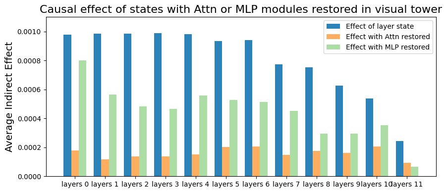
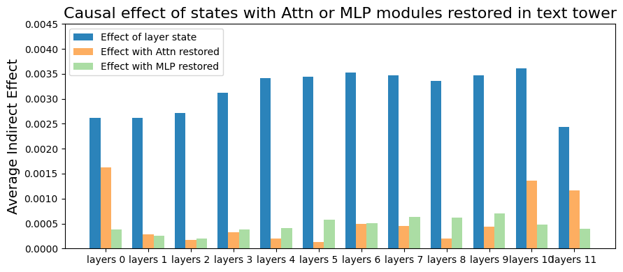
Figure 3: Casual tracking results of visual and text tower of CLIP. Changing MLP layers has higher effect to the CLIP prediction than changing Attention layers.

The figure demonstrates higher $\text{AIE}^{\ell}_{\text{mlp}}$ values compared to $\text{AIE}^{\ell}_{\text{attn}}$ values in both visual and text tower, with a larger contrast in the visual tower. This implies the change of MLP layers contributes more to the final classification, which further validates our choice in performing selection on the MLP layers.

Appendix B Visualization for Parameter Selection

In addition to section 5.3, we further validate the parameter selection qualitatively from two perspectives. Firstly, we utilize gScoreCAM [13] to visualize the attention of selected neurons on original images, illustrating their representativeness to the features. Secondly, we visualize the correlation of selected weights from different tasks. This is to demonstrate the task-wise separation in the selection process, which aids in mitigating forgetting.

gScoreCAM [13] follows the idea of ScoreCAM [54] to perturb the input image with the upsampled activation map, and aggregate the CAM scores. The importance of neuron activations to specific input features is derived from the aggregated scores. gScoreCAM selects only 10% of the activations in regard to their gradient values to perturb the input image, and shows the selected activations are effective in localizing the features. This is in agreement with our selection strategy and modularity hypothesis (section 4). We applied gScoreCAM on the neurons of the first MLP layers in CLIP visual tower and selected the top 10% activation values to perturb the input image. We show the highlighted regions by selected activations of images from the CUB dataset in Figure 4. We perform the visualization on the neurons of the first MLP layers of the 9th transformer layers.

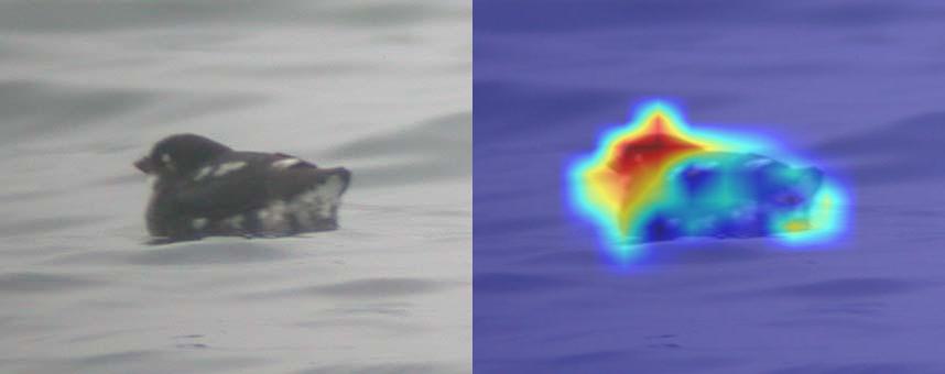
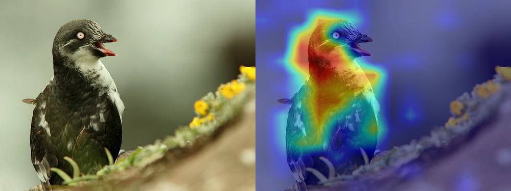
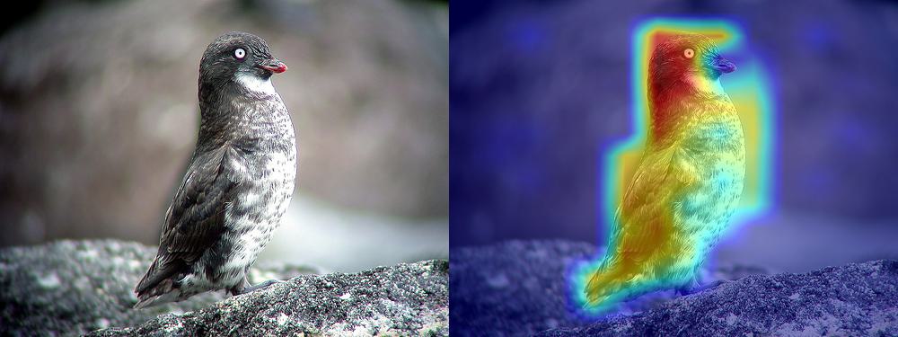
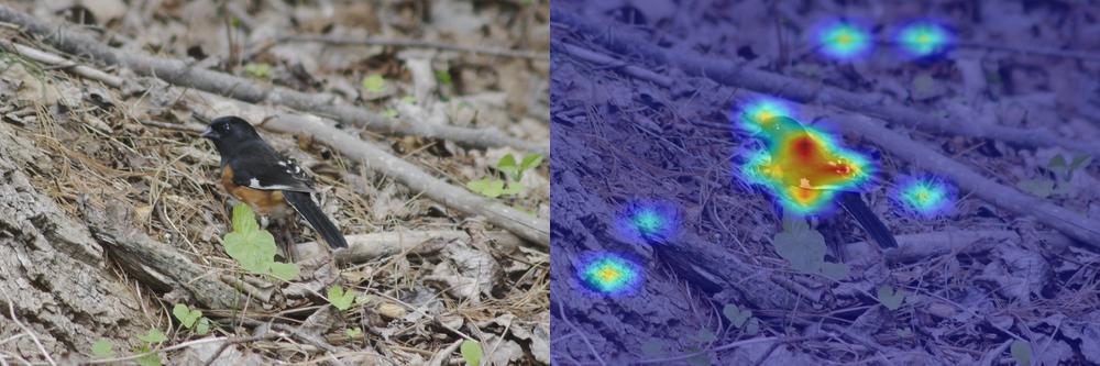
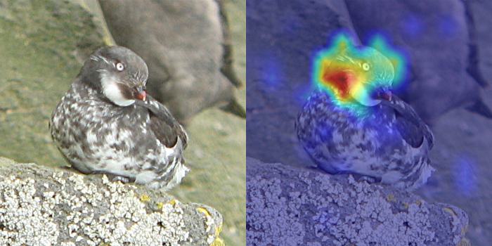
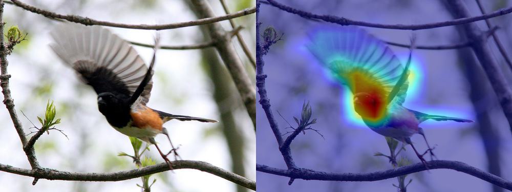
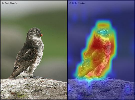
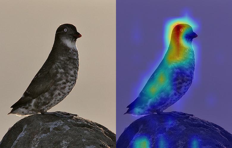
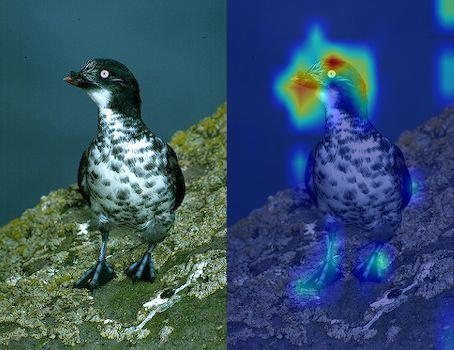
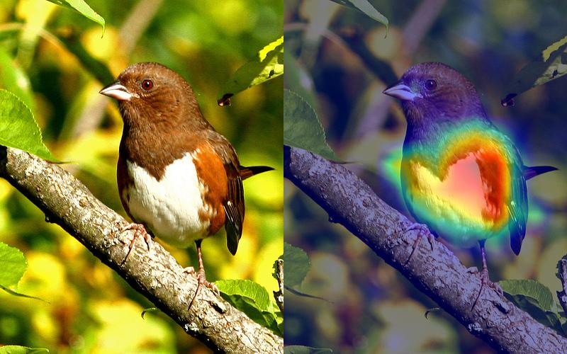
Figure 4: Highlighted regions by activations of selected neurons in the first MLP layers of the 9th transformer block in gScoreCAM visualization. Selected neurons represent meaningful features in the input image.

In Figure  5, we analyze the correlation between selected weights across different tasks in various layers. Patch with row label task $i$ and column label task $j$ shows the percentage of the shared weights selected in task $i$ and task $j$. We observe that the frequency of repeated weight selection for different tasks seldom exceeds 50%. This pattern suggests that while our scoring function occasionally identifies common weights across tasks, it predominantly selects task-specific weights. Notably, the incidence of repeated selection decreases in shallower layers, as demonstrated in layer 5 (first row), which implies a higher occurrence of modulation in these layers. Thus, our approach of selecting weights across all transformer layers is further validated.

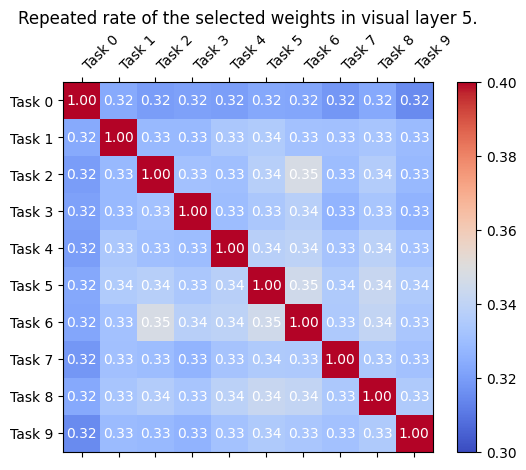
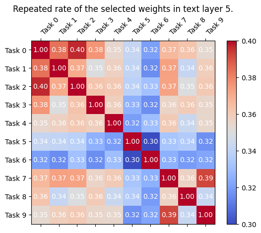
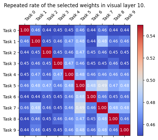
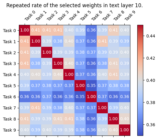
Figure 5: Repeat rate of the selected weight in visual and text tower of layer 5 and layer 10 in CLIP. The shared weight selected two different tasks only counts a small amount of total selected weight.

Appendix C Learnable Scoring Function

In section 5.3, we perform different scoring functions to validate the effectiveness of our proposed gradient-based scoring function, including the Mask baseline. Here, we describe the Mask baseline.

Although the gradient is an efficient approximation of the parameters’ relevance to the task at hand, we suspect selecting parameters independently based on their gradient magnitude might not consider the contribution of the parameters together when updated, and can potentially cause redundancy in the selection. To explore this, we propose to involve an optional optimization stage to adjust the scoring function based on the initial gradient values. Specifically, for parameters $\mathbf{\theta}^{l}\in\mathbb{R}^{m\times n}$, we define ${\bm{S}}\in\mathbb{R}^{m\times n}$ to be the learnable parameters scores. We initialize ${\bm{S}}$ with the gradients computed on the current task, where ${\bm{S}}_{ij}=\frac{1}{N_{t}^{\prime}}\sum_{k=1}^{N_{t}^{\prime}}g_{ij}(x_{k})$. We consider the estimated gradient as the basis for a target update of the model parameters and construct an imaginary update:

$$\theta^{l\prime}=\theta^{l}-\mu\cdot{\bm{S}},$$ (8)

where $\mu$ is the update step size (learning rate). We then optimize ${\bm{S}}$ by minimizing the task loss $\mathcal{L}$ and an additional $L_{1}$ loss ($\|{\bm{S}}\|_{1}$)

$${\bm{S}}^{\prime}=\operatorname*{arg\,min}_{{\bm{S}}}\mathcal{L}(\theta^{l\prime};D^{t})+\lambda\|{\bm{S}}\|_{1},\vspace{-1mm}$$ (9)

where $\lambda$ is a hyperparameter that weighs the contribution of $L_{1}$ loss. $L_{1}$ loss is introduced to encourage sparsity in the estimated scores, guiding the optimization to tolerate parameters with large gradient magnitude (and hence large initial scores) when proven relevant to the minimization of the task loss while zeroing out gradients of irrelevant or redundant parameters.

We optimize ${\bm{S}}$ for a few epochs. Then, we define $\mathcal{S}(\theta^{l}_{ij},D^{t})={\bm{S}}^{\prime}_{i,j}$ and select top $r$ parameters as the most relevant parameters for the task at hand. Note that here we estimate parameter scores for one selected layer $\theta^{l}$, but the formulation can generalize to an arbitrary number of layers.

The learnable scoring function requires more computation due to the additional optimization phase of ${\bm{S}}$ compared to the gradient scores. We present the efficacy of this optional stage in Table 3 of the main paper.

Appendix D Implementation Details

D.1 Dataset

Here are the statistics of our six experimental benchmarks.

Birdsnap [5] Birdsnap is a large bird dataset originally consisting of 49,829 images from 500 bird species with 47,386 images used for training and 2,443 images used for testing. We download the dataset from the official link. We follow the official train-test split. We use a fixed buffer of size 1,500 for this dataset.

CUB-200-2011 [53] The Caltech-UCSD Birds-200-2011 (CUB-200-2011) dataset is for fine-grained visual categorization task. It contains 11,788 images of 200 subcategories belonging to birds, 5,994 for training and 5,794 for testing. We use the Hugging Face implementation of the dataloader. We use a fixed buffer of size 240 for this dataset.

CIFAR100 [31] This dataset has 100 classes containing 600 images each. There are 500 training images and 100 testing images per class. We use the PyTorch implementation of the dataloader. We used a fixed buffer of 2,000 for this dataset.

FGVC-Aircraft [38] The dataset contains 10,200 images of aircraft, with 100 images for each of 102 different aircraft model variants, most of which are airplanes. The data is divided into three equally sized training, validation, and test subsets. We use the PyTorch implementation of the dataloader, where train and valid set are used for training, and the test set is used for testing. We use a fixed buffer of size 250 for this dataset.

Stanford Cars [30] The Cars dataset contains 16,185 images of 196 classes of cars. The data is split into 8,144 training images and 8,041 testing images, where each class has been split roughly in a 50-50 split. Classes are typically at the level of Make, Model, Year, e.g., 2012 Tesla Model S or 2012 BMW M3 coupe. We use the Hugging Face implementation of the dataloader. We use a fixed buffer of size 240 for this dataset.

GTSRB [50] This dataset is designed for recognition of traffic signs. By the time we download it, it contains 43 classes with 26,640 training samples and 12,630 testing samples. We use the PyTorch implementation of the dataloader. We used a fixed buffer of 1,000 for this dataset.

For each dataset, during the training, we use the prompt a photo of {} with class name as text inputs. We evaluate each baseline on the test set using the original prompts and ensembling strategy provided by  Radford et al. [47].

D.2 Hyper-parameters

For our algorithm, we use PyTorch implemented AdamW optimizer  [37] and learning rate scheduler of Cosine Annealing with Warmup  [36] for our algorithm, as well as FLYP combined with ER and other CL regularization methods. We use a learning rate of 7.5e-6 and train for 10 epochs for all datasets. We report results based on an average of 5 different random seeds. We run all our experiments on one single Nvidia A100 GPU.

D.3 Baseline Details

Here are the implementations for other baselines in Table 1.

FLYP [21] For all FLYP based baselines, we tuned the learning rate in [2.5e-6, 5e-6, 7.5e-6] and training epochs in [5,10,15] and report the best results

FLYP+ER [11] For ER-based baselines, we apply balanced sampling, where at each step, we sample a balanced batch, half from the current task and half from the previous tasks.

FLYP + MAS [2] We follow the avalanche  [35] to implement MAS regularizer with FLYP. To cope with the large-scale architecture, we normalize the estimated weights’ importance by their maximum value. We tuned the scaling factor of MAS loss in [0.01, 0.05, 0.1] and report the best results.

FLYP + ER + LwF/PRD  [33, 4] For LwF, we follow the implementation of avalanche. For PRD, we follow the official implementation. We further tuned temperature in [0.01,0.1,1.0,5.0] and loss scaling factor in [0.01, 0.05, 0.1] and report the best results.

L2P, DualPrompt [57, 56] These two methods were originally designed for ViT backbone with linear classifier. They proposed to freeze the feature extractor and only train the classifier. We adopt the idea to the backbone of CLIP architecture, where we freeze the visual and text feature extractors and only train the linear projection layers. We applied the prompt techniques on the visual tower of CLIP. We deploy them with the CLIP pre-trained weights provided by timm library. We further applied a class balanced buffer to them as what we did for FLYP + ER. These methods are highly tailored for ImageNet pretrained transformers and do not scale to other pretrained weights, leading to surprisingly bad performance when combined with CLIP, in spite of our best efforts to tune the hyperparameters carefully.

SLCA [61] We adopted the slow learning rate and classifier alignment to the CLIP backbone. In the first training phase, we applied the learning of $1.5e-6$ to the backbone, and $7.5e-6$ to the projection layers. In the section training phase of classifier alignment, we only train the projection layers.

LoRA-EWC [59] We compute fisher information by CC12m [9], and apply the EWC loss on every task. We applied the LoRA architecture on both visual and text tower. We further modified it with different ranks in LoRA and applied a replay buffer.

Here are other baselines in Table 2.

Random This baseline mainly follows our method SPU, except for Equation 2 in the main paper. In this baseline, we use random values for the scoring function.

Mask We described this method in Section  C in the supplement. We optimize the learnable score matrix ${\bm{S}}$ for 5 epochs, with the learning rate of $5e-4$ and step size $\mu=5e-4$. We set the $L_{1}$ loss coefficient $\lambda=1e-3$

PiggyBack [39] This baseline mainly follows the Mask baseline, except for the format of the imaginary update in Equation 8 in the supplement. We applied the PiggyBack mask learning format, where

$$\theta^{l\prime}=\theta^{l}+\mu\cdot\text{m}({\bm{S}}).$$ (10)

Here $\mu$ is a scaling factor, and $\text{m}(\cdot)$ is a binary mask. We uniformly initialized ${\bm{S}}$ and applied AdamW optimizer as proposed in PiggyBack. We optimize the score matrix ${\bm{S}}$ for 5 epochs, with the learning rate of 1e-4 and the scaling factor $\mu$ of 1e-5.

Appendix E More Details in Ablation Study

Neuron-based Selection.

	Aircraft			Birdsnap			Cars			CIFAR100			CUB			GTSRB			Average
	Acc.	F.	C.	Acc.	F.	C.	Acc.	F.	C.	Acc.	F.	C.	Acc.	F.	C.	Acc.	F.	C.	Acc. In.	Avg. F.	C. Drop
Weight	44.43	14.42	63.48	55.35	12.78	61.94	77.51	3.26	63.42	83.99	-0.39	61.38	71.51	4.84	62.87	94.25	-7.87	62.55	21.34	4.51	0.94
Neuron	44.13	14.02	63.60	55.32	12.66	62.77	77.46	3.33	63.62	83.98	-0.79	61.84	71.14	5.16	63.23	93.54	-8.15	63.22	21.09	4.37	0.50

Table 7: Comparison between weight-based selection and neuron-based selection. Our method employs weight selection and has better learning ability.

We propose to compute the element-wise importance scores by Equation 2 in the main paper to facilitate weight-based selection. Whereas,  Aljundi et al. [3] put forth a technique to calculate row-wise importance scores to perform neuron-based selection.

Table  7 shows the full results of variants of selection strategy, where the gray row represents our strategy. In the baseline named “Weight” we compute an element-wise scoring function by Equation 2, and select the top 10% entries of each weight matrix to update. In the baseline named “Neuron”, we compute a row-wise scoring function based on the row summation of the element-wise scoring function by Equation 2. Then we select the 10% rows of each weight matrix to update.

We find that weight-based selection yields slightly improved learning performance while exhibiting a marginal decrease in hold-out accuracy. Nonetheless, the overall performance trends remain comparable between the two strategies. This observation highlights the robustness of our localization and importance scoring methods to any of the selection strategy.

Selection Rate.

In Section 5.3, we present the average results of our method under varying selection rates. Table  8 shows the full results, where the gray row represents our reported results. Our main results select the top 10% elements localized layer. We compare to the baselines where the top 1% or the top 50% are selected for update. All other configurations are kept the same.

	Aircraft			Birdsnap			Cars			CIFAR100			CUB			GTSRB			Average
	Acc.	F.	C.	Acc.	F.	C.	Acc.	F.	C.	Acc.	F.	C.	Acc.	F.	C.	Acc.	F.	C.	Acc. In.	Avg. F.	C. Drop
0.01	37.64	11.45	63.54	53.49	9.87	62.25	74.62	2.20	63.40	83.79	-1.64	60.91	66.79	4.39	63.01	88.89	-7.71	61.53	17.70	3.10	1.11
0.10	44.43	14.42	63.48	55.35	12.78	61.94	77.51	3.26	63.42	83.99	-0.39	61.38	71.51	4.84	62.87	94.25	-7.87	62.55	21.34	4.51	0.94
0.50	46.73	20.74	63.56	53.96	17.98	61.72	77.64	6.12	63.48	83.47	1.51	61.53	71.89	8.06	62.85	95.74	-7.85	62.43	21.73	7.76	0.95

Table 8: Full results of ablation on selection rate. Our method select 10% weights, achieving better trade-off in learning and forgetting.

Buffer Size.

In Section 5.3, we present the average results of our method and FLYP + ER under varying buffer size. We study buffer sizes of 1%, 2% and 4% of the total dataset size. Table  9 shows the full results of buffer size ablation. We report our method with 4% buffer size of the total dataset size in Table 1 in the main paper, highlighted in gray.

Method	Buffer Size / Total Size	Aircraft			Birdsnap			Cars			CIFAR100			CUB			GTSRB			Average
		Acc.	F.	C.	Acc.	F.	C.	Acc.	F.	C.	Acc.	F.	C.	Acc.	F.	C.	Acc.	F.	C.	Acc. In.	Avg. F.	C. Drop
ER	1%	27.76	44.49	49.22	43.76	33.59	55.90	61.22	21.19	55.34	73.70	13.34	40.14	53.39	25.26	48.81	93.03	-4.22	16.79	8.97	22.27	19.18
ER	2%	33.42	41.37	49.74	49.96	29.20	56.35	62.83	21.45	57.35	78.72	7.94	41.74	57.90	22.84	50.83	95.64	-6.68	15.82	13.24	19.35	18.24
ER	4%	41.42	31.48	50.41	56.22	21.63	56.72	69.08	16.42	58.07	82.86	3.41	42.10	64.07	17.72	51.30	96.28	-7.40	17.34	18.48	13.88	17.56
SPU	1%	37.82	21.96	63.56	47.54	23.61	61.65	73.68	6.84	63.36	80.44	4.87	61.49	66.06	9.32	62.47	90.55	-4.93	62.76	16.18	10.28	1.00
SPU	2%	40.65	20.31	63.44	51.33	18.97	61.90	75.00	6.17	63.41	82.45	2.03	61.36	68.39	8.42	62.81	92.99	-7.04	62.63	18.63	8.14	0.96
SPU	4%	44.43	14.42	63.48	55.35	12.78	61.94	77.51	3.26	63.42	83.99	-0.39	61.38	71.51	4.84	62.87	94.25	-7.87	62.55	21.34	4.51	0.94

Table 9: Full results of ablation on the buffer size. Our method shows superior performance over ER even in smaller buffer scenarios.

Appendix F More Details in Efficiency

	Aircraft			Birdsnap			Cars			CIFAR100			CUB			GTSRB			Average
	Acc.	F.	C.	Acc.	F.	C.	Acc.	F.	C.	Acc.	F.	C.	Acc.	F.	C.	Acc.	F.	C.	Acc. In.	Avg. F.	C. Drop
one batch	44.42	14.40	63.50	55.02	13.33	62.04	77.41	3.36	63.40	83.99	-0.38	61.36	71.48	4.90	62.86	94.14	-7.79	62.52	21.24	4.64	0.94
0.25	44.43	14.42	63.48	55.35	12.78	61.94	77.51	3.26	63.42	83.99	-0.39	61.38	71.51	4.84	62.87	94.25	-7.87	62.55	21.34	4.51	0.94
0.50	44.33	14.48	63.48	55.31	12.73	61.88	77.54	3.16	63.44	84.03	-0.41	61.37	71.67	4.63	62.87	94.24	-7.82	62.58	21.35	4.46	0.94
1.00	44.40	14.40	63.47	55.28	12.61	61.85	77.61	3.12	63.44	84.05	-0.40	61.35	71.66	4.64	62.87	94.27	-7.81	62.58	21.37	4.43	0.96

Table 10: Full results of ablation on the number of samples to compute the gradient approximation. Our scoring function can efficiently cope with only one-batch gradient accumulation.

Number of samples to compute gradient approximation.

In Equation 2, we accumulate the gradients of $N^{\prime}_{t}$ samples to approximate the importance. Here we ablate the effect of accumulating gradients with one batch (128 data points), 25% 50%, and 100% of the current set. We compute the importance score by the accumulated gradients before the training of every task, and the computational cost per task gets reduced with fewer samples to approximate the scoring function. With more samples, the accuracy is slightly increased, with also slight decrease in forgetting. Our algorithm is robust to all different configurations in general. Full results are shown in Table  10. We choose to report our main results by accumulate gradients of 25% samples of the current set, highlighted in gray.

References

- Alayrac et al. [2022] Jean-Baptiste Alayrac, Jeff Donahue, Pauline Luc, Antoine Miech, Iain Barr, Yana Hasson, Karel Lenc, Arthur Mensch, Katherine Millican, Malcolm Reynolds, Roman Ring, Eliza Rutherford, Serkan Cabi, Tengda Han, Zhitao Gong, Sina Samangooei, Marianne Monteiro, Jacob Menick, Sebastian Borgeaud, Andrew Brock, Aida Nematzadeh, Sahand Sharifzadeh, Mikolaj Binkowski, Ricardo Barreira, Oriol Vinyals, Andrew Zisserman, and Karen Simonyan. Flamingo: a visual language model for few-shot learning. In Advances in Neural Information Processing Systems, 2022.
- Aljundi et al. [2018] Rahaf Aljundi, Francesca Babiloni, Mohamed Elhoseiny, Marcus Rohrbach, and Tinne Tuytelaars. Memory aware synapses: Learning what (not) to forget. In European Conference on Computer Vision (ECCV), 2018.
- Aljundi et al. [2019] Rahaf Aljundi, Marcus Rohrbach, and Tinne Tuytelaars. Selfless sequential learning. In International Conference on Learning Representations, 2019.
- Asadi et al. [2023] Nader Asadi, MohammadReza Davari, Sudhir Mudur, Rahaf Aljundi, and Eugene Belilovsky. Prototype-sample relation distillation: Towards replay-free continual learning. In International Conference on Machine Learning, pages 1093–1106. PMLR, 2023.
- Berg et al. [2014] Thomas Berg, Jiongxin Liu, Seung Woo Lee, Michelle L Alexander, David W Jacobs, and Peter N Belhumeur. Birdsnap: Large-scale fine-grained visual categorization of birds. In Proceedings of the IEEE Conference on Computer Vision and Pattern Recognition, pages 2011–2018, 2014.
- Bills et al. [2023] Steven Bills, Nick Cammarata, Dan Mossing, Henk Tillman, Leo Gao, Gabriel Goh, Ilya Sutskever, Jan Leike, Jeff Wu, and William Saunders. Language models can explain neurons in language models. https://openaipublic.blob.core.windows.net/neuron-explainer/paper/index.html, 2023.
- Bommasani et al. [2021] Rishi Bommasani, Drew A Hudson, Ehsan Adeli, Russ Altman, Simran Arora, Sydney von Arx, Michael S Bernstein, Jeannette Bohg, Antoine Bosselut, Emma Brunskill, et al. On the opportunities and risks of foundation models. arXiv preprint arXiv:2108.07258, 2021.
- Caccia et al. [2020] Massimo Caccia, Pau Rodríguez, Oleksiy Ostapenko, Fabrice Normandin, Min Lin, Lucas Caccia, Issam Laradji, Irina Rish, Alexandre Lacoste, David Vazquez, and Laurent Charlin. Online fast adaptation and knowledge accumulation (osaka): A new approach to continual learning. In Proceedings of the 34th International Conference on Neural Information Processing Systems, Red Hook, NY, USA, 2020. Curran Associates Inc.
- Changpinyo et al. [2021] Soravit Changpinyo, Piyush Sharma, Nan Ding, and Radu Soricut. Conceptual 12M: Pushing web-scale image-text pre-training to recognize long-tail visual concepts. In CVPR, 2021.
- Chaudhry et al. [2019a] Arslan Chaudhry, Marc’Aurelio Ranzato, Marcus Rohrbach, and Mohamed Elhoseiny. Efficient lifelong learning with a-gem. In ICLR, 2019a.
- Chaudhry et al. [2019b] Arslan Chaudhry, Marcus Rohrbach, Mohamed Elhoseiny, Thalaiyasingam Ajanthan, Puneet K. Dokania, Philip H. S. Torr, and Marc’Aurelio Ranzato. On tiny episodic memories in continual learning, 2019b.
- Chen et al. [2022a] Jun Chen, Han Guo, Kai Yi, Boyang Li, and Mohamed Elhoseiny. Visualgpt: Data-efficient adaptation of pretrained language models for image captioning. In Proceedings of the IEEE/CVF Conference on Computer Vision and Pattern Recognition, pages 18030–18040, 2022a.
- Chen et al. [2022b] Peijie Chen, Qi Li, Saad Biaz, Trung Bui, and Anh Nguyen. gscorecam: What objects is clip looking at? In Proceedings of the Asian Conference on Computer Vision, pages 1959–1975, 2022b.
- Dar et al. [2022] Guy Dar, Mor Geva, Ankit Gupta, and Jonathan Berant. Analyzing transformers in embedding space, 2022.
- Deng et al. [2009] Jia Deng, Wei Dong, Richard Socher, Li-Jia Li, Kai Li, and Li Fei-Fei. Imagenet: A large-scale hierarchical image database. In 2009 IEEE Conference on Computer Vision and Pattern Recognition, pages 248–255, 2009.
- Driess et al. [2023] Danny Driess, Fei Xia, Mehdi SM Sajjadi, Corey Lynch, Aakanksha Chowdhery, Brian Ichter, Ayzaan Wahid, Jonathan Tompson, Quan Vuong, Tianhe Yu, et al. Palm-e: An embodied multimodal language model. arXiv preprint arXiv:2303.03378, 2023.
- Ebrahimi et al. [2019] Sayna Ebrahimi, Mohamed Elhoseiny, Trevor Darrell, and Marcus Rohrbach. Uncertainty-guided continual learning with bayesian neural networks. In International Conference on Learning Representations, 2019.
- Ebrahimi et al. [2020] Sayna Ebrahimi, Franziska Meier, Roberto Calandra, Trevor Darrell, and Marcus Rohrbach. Adversarial continual learning. In European Conference on Computer Vision (ECCV), 2020.
- Geva et al. [2021] Mor Geva, Roei Schuster, Jonathan Berant, and Omer Levy. Transformer feed-forward layers are key-value memories. In Empirical Methods in Natural Language Processing (EMNLP), 2021.
- Geva et al. [2022] Mor Geva, Avi Caciularu, Kevin Wang, and Yoav Goldberg. Transformer feed-forward layers build predictions by promoting concepts in the vocabulary space. In Proceedings of the 2022 Conference on Empirical Methods in Natural Language Processing, pages 30–45, Abu Dhabi, United Arab Emirates, 2022. Association for Computational Linguistics.
- Goyal et al. [2023] Sachin Goyal, Ananya Kumar, Sankalp Garg, Zico Kolter, and Aditi Raghunathan. Finetune like you pretrain: Improved finetuning of zero-shot vision models. In Proceedings of the IEEE/CVF Conference on Computer Vision and Pattern Recognition, pages 19338–19347, 2023.
- Hartvigsen et al. [2022] Thomas Hartvigsen, Swami Sankaranarayanan, Hamid Palangi, Yoon Kim, and Marzyeh Ghassemi. Aging with grace: Lifelong model editing with discrete key-value adaptors. arXiv preprint arXiv:2211.11031, 2022.
- He et al. [2021] Junxian He, Chunting Zhou, Xuezhe Ma, Taylor Berg-Kirkpatrick, and Graham Neubig. Towards a unified view of parameter-efficient transfer learning. In International Conference on Learning Representations, 2021.
- Hu et al. [2022] Edward J Hu, yelong shen, Phillip Wallis, Zeyuan Allen-Zhu, Yuanzhi Li, Shean Wang, Lu Wang, and Weizhu Chen. LoRA: Low-rank adaptation of large language models. In International Conference on Learning Representations, 2022.
- Ilharco et al. [2022] Gabriel Ilharco, Marco Tulio Ribeiro, Mitchell Wortsman, Ludwig Schmidt, Hannaneh Hajishirzi, and Ali Farhadi. Editing models with task arithmetic. In The Eleventh International Conference on Learning Representations, 2022.
- Janson et al. [2022] Paul Janson, Wenxuan Zhang, Rahaf Aljundi, and Mohamed Elhoseiny. A simple baseline that questions the use of pretrained-models in continual learning. In NeurIPS 2022 Workshop on Distribution Shifts: Connecting Methods and Applications, 2022.
- Jia et al. [2022] Menglin Jia, Luming Tang, Bor-Chun Chen, Claire Cardie, Serge Belongie, Bharath Hariharan, and Ser-Nam Lim. Visual prompt tuning. In European Conference on Computer Vision, pages 709–727. Springer, 2022.
- Khattak et al. [2023] Muhammad Uzair Khattak, Syed Talal Wasim, Muzammal Naseer, Salman Khan, Ming-Hsuan Yang, and Fahad Shahbaz Khan. Self-regulating prompts: Foundational model adaptation without forgetting. arXiv preprint arXiv:2307.06948, 2023.
- Kirkpatrick et al. [2017] James Kirkpatrick, Razvan Pascanu, Neil Rabinowitz, Joel Veness, Guillaume Desjardins, Andrei A Rusu, Kieran Milan, John Quan, Tiago Ramalho, Agnieszka Grabska-Barwinska, et al. Overcoming catastrophic forgetting in neural networks. Proceedings of the national academy of sciences, 114(13):3521–3526, 2017.
- Krause et al. [2013] Jonathan Krause, Michael Stark, Jia Deng, and Li Fei-Fei. 3d object representations for fine-grained categorization. In Proceedings of the IEEE international conference on computer vision workshops, pages 554–561, 2013.
- Krizhevsky et al. [2009] Alex Krizhevsky, Geoffrey Hinton, et al. Learning multiple layers of features from tiny images. 2009.
- Li et al. [2023] Junnan Li, Dongxu Li, Silvio Savarese, and Steven Hoi. Blip-2: Bootstrapping language-image pre-training with frozen image encoders and large language models, 2023.
- Li and Hoiem [2017] Zhizhong Li and Derek Hoiem. Learning without forgetting. IEEE transactions on pattern analysis and machine intelligence, 40(12):2935–2947, 2017.
- Lin et al. [2014] Tsung-Yi Lin, Michael Maire, Serge Belongie, James Hays, Pietro Perona, Deva Ramanan, Piotr Dollár, and C Lawrence Zitnick. Microsoft coco: Common objects in context. In Computer Vision–ECCV 2014: 13th European Conference, Zurich, Switzerland, September 6-12, 2014, Proceedings, Part V 13, pages 740–755. Springer, 2014.
- Lomonaco et al. [2021] Vincenzo Lomonaco, Lorenzo Pellegrini, Andrea Cossu, Antonio Carta, Gabriele Graffieti, Tyler L. Hayes, Matthias De Lange, Marc Masana, Jary Pomponi, Gido van de Ven, Martin Mundt, Qi She, Keiland Cooper, Jeremy Forest, Eden Belouadah, Simone Calderara, German I. Parisi, Fabio Cuzzolin, Andreas Tolias, Simone Scardapane, Luca Antiga, Subutai Amhad, Adrian Popescu, Christopher Kanan, Joost van de Weijer, Tinne Tuytelaars, Davide Bacciu, and Davide Maltoni. Avalanche: an end-to-end library for continual learning. In Proceedings of IEEE Conference on Computer Vision and Pattern Recognition, 2021.
- Loshchilov and Hutter [2016] Ilya Loshchilov and Frank Hutter. Sgdr: Stochastic gradient descent with warm restarts. arXiv preprint arXiv:1608.03983, 2016.
- Loshchilov and Hutter [2017] Ilya Loshchilov and Frank Hutter. Decoupled weight decay regularization. arXiv preprint arXiv:1711.05101, 2017.
- Maji et al. [2013] S. Maji, J. Kannala, E. Rahtu, M. Blaschko, and A. Vedaldi. Fine-grained visual classification of aircraft. Technical report, 2013.
- Mallya et al. [2018] Arun Mallya, Dillon Davis, and Svetlana Lazebnik. Piggyback: Adapting a single network to multiple tasks by learning to mask weights. In Proceedings of the European conference on computer vision (ECCV), pages 67–82, 2018.
- McCloskey and Cohen [1989] Michael McCloskey and Neal J Cohen. Catastrophic interference in connectionist networks: The sequential learning problem. In Psychology of learning and motivation, pages 109–165. Elsevier, 1989.
- Meng et al. [2022a] Kevin Meng, David Bau, Alex Andonian, and Yonatan Belinkov. Locating and editing factual associations in gpt. Advances in Neural Information Processing Systems, 35:17359–17372, 2022a.
- Meng et al. [2022b] Kevin Meng, Arnab Sen Sharma, Alex J Andonian, Yonatan Belinkov, and David Bau. Mass-editing memory in a transformer. In The Eleventh International Conference on Learning Representations, 2022b.
- Mitchell et al. [2022] Eric Mitchell, Charles Lin, Antoine Bosselut, Chelsea Finn, and Christopher D Manning. Fast model editing at scale. In International Conference on Learning Representations, 2022.
- Onoe et al. [2023] Yasumasa Onoe, Michael JQ Zhang, Shankar Padmanabhan, Greg Durrett, and Eunsol Choi. Can lms learn new entities from descriptions? challenges in propagating injected knowledge. arXiv preprint arXiv:2305.01651, 2023.
- OpenAI [2023] OpenAI. Gpt-4 technical report, 2023.
- Parisi et al. [2019] German I Parisi, Ronald Kemker, Jose L Part, Christopher Kanan, and Stefan Wermter. Continual lifelong learning with neural networks: A review. Neural networks, 113:54–71, 2019.
- Radford et al. [2021] Alec Radford, Jong Wook Kim, Chris Hallacy, Aditya Ramesh, Gabriel Goh, Sandhini Agarwal, Girish Sastry, Amanda Askell, Pamela Mishkin, Jack Clark, et al. Learning transferable visual models from natural language supervision. In International conference on machine learning, pages 8748–8763. PMLR, 2021.
- Santurkar et al. [2021] Shibani Santurkar, Dimitris Tsipras, Mahalaxmi Elango, David Bau, Antonio Torralba, and Aleksander Madry. Editing a classifier by rewriting its prediction rules. In Advances in Neural Information Processing Systems, 2021.
- Smith et al. [2023] James Seale Smith, Leonid Karlinsky, Vyshnavi Gutta, Paola Cascante-Bonilla, Donghyun Kim, Assaf Arbelle, Rameswar Panda, Rogerio Feris, and Zsolt Kira. Coda-prompt: Continual decomposed attention-based prompting for rehearsal-free continual learning. In Proceedings of the IEEE/CVF Conference on Computer Vision and Pattern Recognition, pages 11909–11919, 2023.
- Stallkamp et al. [2012] Johannes Stallkamp, Marc Schlipsing, Jan Salmen, and Christian Igel. Man vs. computer: Benchmarking machine learning algorithms for traffic sign recognition. Neural networks, 32:323–332, 2012.
- Steiner et al. [2021] Andreas Steiner, Alexander Kolesnikov, , Xiaohua Zhai, Ross Wightman, Jakob Uszkoreit, and Lucas Beyer. How to train your vit? data, augmentation, and regularization in vision transformers. arXiv preprint arXiv:2106.10270, 2021.
- Vig et al. [2020] Jesse Vig, Sebastian Gehrmann, Yonatan Belinkov, Sharon Qian, Daniel Nevo, Yaron Singer, and Stuart Shieber. Investigating gender bias in language models using causal mediation analysis. Advances in neural information processing systems, 33:12388–12401, 2020.
- Wah et al. [2011] Catherine Wah, Steve Branson, Peter Welinder, Pietro Perona, and Serge Belongie. The caltech-ucsd birds-200-2011 dataset. 2011.
- Wang et al. [2020] Haofan Wang, Zifan Wang, Mengnan Du, Fan Yang, Zijian Zhang, Sirui Ding, Piotr Mardziel, and Xia Hu. Score-cam: Score-weighted visual explanations for convolutional neural networks. In Proceedings of the IEEE/CVF conference on computer vision and pattern recognition workshops, pages 24–25, 2020.
- Wang et al. [2022a] Yabin Wang, Zhiwu Huang, and Xiaopeng Hong. S-prompts learning with pre-trained transformers: An occam’s razor for domain incremental learning. In Conference on Neural Information Processing Systems (NeurIPS), 2022a.
- Wang et al. [2022b] Zifeng Wang, Zizhao Zhang, Sayna Ebrahimi, Ruoxi Sun, Han Zhang, Chen-Yu Lee, Xiaoqi Ren, Guolong Su, Vincent Perot, Jennifer Dy, et al. Dualprompt: Complementary prompting for rehearsal-free continual learning. European Conference on Computer Vision, 2022b.
- Wang et al. [2022c] Zifeng Wang, Zizhao Zhang, Chen-Yu Lee, Han Zhang, Ruoxi Sun, Xiaoqi Ren, Guolong Su, Vincent Perot, Jennifer Dy, and Tomas Pfister. Learning to prompt for continual learning. In Proceedings of the IEEE/CVF Conference on Computer Vision and Pattern Recognition (CVPR), pages 139–149, 2022c.
- Wightman [2019] Ross Wightman. Pytorch image models. https://github.com/huggingface/pytorch-image-models, 2019.
- Xiang et al. [2023] Jiannan Xiang, Tianhua Tao, Yi Gu, Tianmin Shu, Zirui Wang, Zichao Yang, and Zhiting Hu. Language models meet world models: Embodied experiences enhance language models. arXiv preprint arXiv:2305.10626, 2023.
- Xu et al. [2023] Peng Xu, Wenqi Shao, Kaipeng Zhang, Peng Gao, Shuo Liu, Meng Lei, Fanqing Meng, Siyuan Huang, Yu Qiao, and Ping Luo. Lvlm-ehub: A comprehensive evaluation benchmark for large vision-language models. arXiv preprint arXiv:2306.09265, 2023.
- Zhang et al. [2023] Gengwei Zhang, Liyuan Wang, Guoliang Kang, Ling Chen, and Yunchao Wei. Slca: Slow learner with classifier alignment for continual learning on a pre-trained model. In Proceedings of the IEEE/CVF International Conference on Computer Vision (ICCV), pages 19148–19158, 2023.
- Zheng et al. [2023] Zangwei Zheng, Mingyuan Ma, Kai Wang, Ziheng Qin, Xiangyu Yue, and Yang You. Preventing zero-shot transfer degradation in continual learning of vision-language models. In ICCV, 2023.