Pion Transition Form Factor from Twisted-Mass Lattice QCD
and the Hadronic Light-by-Light $\pi^{0}$-pole Contribution to the Muon $g-2$

Abstract

The neutral pion generates the leading pole contribution to the hadronic light-by-light tensor, which is given in terms of the nonperturbative transition form factor $\mathcal{F}_{\pi^{0}\gamma\gamma}(q_{1}^{2},q_{2}^{2})$. Here we present an ab-initio lattice calculation of this quantity in the continuum and at the physical point using twisted-mass lattice QCD. We report our results for the transition form factor parameterized using a model-independent conformal expansion valid for arbitrary space-like kinematics and compare it with experimental measurements of the single-virtual form factor, the two-photon decay width, and the slope parameter. We then use the transition form factors to compute the pion-pole contribution to the hadronic light-by-light scattering in the muon $g-2$, finding $a_{\mu}^{\pi^{0}-\mathrm{pole}}=56.7(3.2)\times 10^{-11}$.

I Introduction

The anomalous magnetic moment of the muon (the muon $g-2$) provides a stringent test of the Standard Model at high precision and the possibility to glimpse subtle effects of potential new physics beyond the Standard Model. Recent results from the Fermilab experiment PhysRevLett.126.141801 ; Muong-2:2023cdq in combination with the Brookhaven result Bennett:2006fi have yielded the most precise experimental determination to date at the level of 19 ppm: $a_{\mu}(\text{exp})=116\,592\,059(22)\times 10^{-11}$, where $a_{\mu}\equiv(g-2)_{\mu}/2$. A comparable precision is striven for on the theoretical side with the recent state of affairs summarized in the white paper Aoyama:2020ynm .

The leading hadronic contributions to the muon anomalous magnetic moment come from diagrams involving the hadronic vacuum polarization (HVP) and the hadronic light-by-light (HLbL) scattering tensors. Both make significant contributions at the level of precision achieved by the experimental results. It is important to improve the theoretical determinations of both contributions to match future targets of experimental precision; this work addresses the HLbL contribution.

Two complementary approaches to the theoretical determination of the HLbL contribution are becoming recognizable for reliable estimates. On one hand, several direct lattice calculations have analyzed the complete HLbL tensor Blum:2014oka ; Blum:2015gfa ; Blum:2016lnc ; Blum:2017cer ; Chao2021 ; Chao:2022xzg ; Asmussen2022 . On the other hand, the HLbL tensor can be decomposed into contributions from exchanges of various intermediate on-shell states in a data-driven dispersive approach, where contributions from heavier intermediate states are suppressed Colangelo2014a ; Colangelo:2014pva ; Colangelo:2015ama ; Pauk:2014rfa . The latter approach has provided the most precise theoretical estimates of the HLbL contribution to the muon $g-2$ to date Aoyama:2020ynm , while the former has the benefit of allowing for a fully self-contained lattice QCD calculation from first principles without resorting to chiral effective field theory and experimental data. However, there has been an ongoing effort to provide also ab-initio data based on lattice QCD calculations for the leading contributions within the dispersive decomposition of the HLbL.

tff/.style= /tikz/shape=circle, /tikz/draw=black, /tikz/pattern=north east lines

blob/.style= /tikz/shape=circle, /tikz/minimum size=1cm, /tikz/draw=black, /tikz/pattern=north east lines

Figure 1: Pseudoscalar-pole diagrams contributing to the leading order hadronic light-by-light (HLbL )scattering. Each striped circle represents a nonperturbative $P\rightarrow\gamma^{*}\gamma^{*}$ transition form factor required to evaluate these contributions, where “$P$” indicates the exchanged pseudoscalar meson. The “flipped” contribution signifies the diagram with the pseudoscalar and photon portions of the diagram horizontally flipped.

The leading single-pole contributions to the HLbL component of the muon $g-2$ arise from the exchange of neutral pseudoscalar mesons $P\in\{\pi^{0},\eta,\eta^{\prime}\}$ as shown in FIG. 1. The key nonperturbative input to these diagrams are the transition form factors (TFFs) $\mathcal{F}_{P\gamma\gamma}(q_{1}^{2},q_{2}^{2})$, defined by Knecht:2001qf

$$\epsilon_{\mu\nu\alpha\beta}q^{\alpha}p^{\beta}\mathcal{F}_{P\gamma\gamma}(q_{1}^{2},q_{2}^{2})\equiv M_{\mu\nu}(p,q_{1})$$ (1)

$$\hskip 40.0pt=i\int d^{4}xe^{iq_{1}x}\langle 0|T\{j_{\mu}(x)j_{\nu}(0)\}|P(p)\rangle,$$

where

$$j_{\mu}(x)=\overline{\psi}(x)\gamma_{\mu}Q\psi(x)$$ (2)

is the electromagnetic current written in terms of the charge matrix $Q$. The momentum of the pseudoscalar meson satisfies the on-shell condition $p^{2}=M_{P}^{2}$, while the photon momenta $q_{1}$ and $q_{2}=p-q_{1}$ may be either on-shell or virtual. The pole contribution to the HLbL tensor from the pseudoscalar meson $P$ is given by

$$\Pi^{(P)}_{\mu\nu\lambda\rho}(q_{1},q_{2},q_{3}) =i\frac{\mathcal{F}_{P\gamma\gamma}(q_{1}^{2},q_{2}^{2})\mathcal{F}_{P\gamma\gamma}(q_{3}^{2},(q_{1}+q_{2}+q_{3})^{2})}{(q_{1}+q_{2})^{2}-M_{P}^{2}}$$ (3)

$$\quad\times\epsilon_{\mu\nu\alpha\beta}q_{1}^{\alpha}q_{2}^{\beta}\epsilon_{\lambda\rho\sigma\tau}q_{3}^{\sigma}(q_{1}+q_{2})^{\tau}$$

$$\quad+(q_{1}\leftrightarrow q_{3})+(q_{2}\leftrightarrow q_{3}).$$

Integrating over space-like $q_{1}$, $q_{2}$, and $q_{3}=-q_{1}-q_{2}$ with the appropriate kinematical factors from the diagrams in FIG. 1 yields contributions to the total muon $g-2$ from each pseudoscalar meson exchange.

The $\pi^{0}$-pole contribution to the muon $g-2$ is larger than those of the $\eta$ and $\eta^{\prime}$ by roughly a factor of four PhysRevD.94.053006 ; Jegerlehner2009 . This feature, together with the relative simplicity of accessing the pion TFF in both lattice and data-driven approaches, means that the study of this transition form factor is farthest advanced at this point. Direct experimental data for $\mathcal{F}_{\pi^{0}\gamma\gamma}(q_{1}^{2},q_{2}^{2})$ is primarily available in the singly virtual (either $q_{1}^{2}=0$ or $q_{2}^{2}=0$) regime with large photon virtuality CELLO:1990klc ; CLEO:1997fho ; BaBar:2009rrj ; BaBar:2011nrp ; Belle:Uehara2012 . Fits to this data using Canterbury approximants have yielded a data-based estimate across all virtualities Masjuan2017a . Meanwhile, the pion TFF has also been determined from indirect experimental data using a dispersive approach Hoferichter:2018dmo ; Hoferichter:2018kwz . On the other hand, an ab-initio determination is desirable to remove the dependence on experimental inputs. As such, the neutral pseudoscalar meson TFF has also been computed on the lattice. The calculation of the neutral-pion TFF on the lattice has been pioneered by the Mainz group using Wilson quarks Gerardin:2016cqj ; Gerardin:2019vio . The BMW collaboration recently added their results using staggered quarks Gerardin:2023naa . Our preliminary results with Wilson twisted-mass quarks appeared in Refs. Burri:2021cxr ; BurriPoS2022 . The major sources of uncertainty in these approaches is the extrapolation to the continuum and, in case the quark masses are not tuned to their physical values as in Refs. Gerardin:2016cqj ; Gerardin:2019vio , the extrapolation to the physical point. A first calculation of the $\eta$-meson TFF and the corresponding pole contribution at one lattice spacing has been reported by our collaboration in Ref. Alexandrou:2022qyf and results for both the $\eta$- and $\eta^{\prime}$-meson TFF and pole contributions addressing all systematic errors have been presented by the BMW collaboration in Ref. Gerardin:2023naa .

In the present work, we complement these existing efforts by evaluating the pion transition form factor in the continuum using the twisted-mass lattice QCD discretization, with ensembles generated directly at the physical point. This calculation serves to strengthen the lattice consensus of the continuum limit and minimizes systematic effects from extrapolation of the pion mass. In this work, we present a parameterization of the pion transition form factor and use it to calculate the $\pi^{0}$-pole contribution to the muon $g-2$. As our main result, we find $a_{\mu}^{\pi^{0}-\mathrm{pole}}=56.7(3.2)\times 10^{-11}$. We further use the transition form factor to estimate the two-photon decay width as $\Gamma(\pi\to\gamma\gamma)=7.50(0.50)\,\mathrm{eV}$, and the slope parameter as $b_{\pi}=2.16(0.20)\,\mathrm{GeV}^{-2}$, which provides input for determining the electromagnetic interaction radius. Quoted uncertainties include statistical errors and systematic uncertainty from analysis choices and the continuum extrapolation.

The structure of this paper is as follows. In Sec. II, we review the theoretical background for the extraction of the required amplitude from lattice QCD simulations. In Sec. III, we describe the calculation of the transition form factors and their extrapolation to photon virtualities required for the observables that we calculate. In Sec. IV, we present the calculation of $a_{\mu}^{\pi^{0}-\mathrm{pole}}$ from the transition form factors and the determination of the decay width $\Gamma(\pi\to\gamma\gamma)$ and the slope parameter $b_{\pi}$. Next, in Sec. V, we discuss the estimation of statistical and systematic errors based on model averaging, before presenting our results in Sec. VI, comparing them to experimental and theoretical predictions. Then, in Sec. VIII, we make some concluding remarks and give an outlook on possible future directions for improving the calculation presented here.

II Euclidean amplitude

By analytic continuation, the Minkowski neutral pion transition form factor in Eq. (1) is related to the Euclidean amplitude

$$\tilde{A}_{\mu\nu}(\tau)=\left<0\big{|}T\{j_{\mu}(\vec{q}_{1},\tau)j_{\nu}(\vec{p}-\vec{q}_{1},0)\}\big{|}\pi^{0}(p)\right>$$ (4)

by Ji:2001wha ; Ji:2001nf ; Dudek:2006ut

$$M_{\mu\nu}(p,q_{1})=i^{n_{0}}M_{\mu\nu}^{E}(p,q_{1}),\quad M_{\mu\nu}^{E}=\int_{-\infty}^{\infty}d\tau\,e^{\omega_{1}\tau}\tilde{A}_{\mu\nu}(\tau),$$ (5)

where $n_{0}=\delta_{\mu,0}+\delta_{\nu,0}$, $q_{1}=(\omega_{1},\vec{q}_{1})$, and $\tau$ indicates a Euclidean time coordinate. Note that $\tilde{A}_{\mu\nu}$ depends on the momenta $\vec{q}_{1}$ and $\vec{p}$, but this dependence is suppressed for conciseness of notation. The analytic continuation is valid for virtualities $q^{2}_{1}$ and $q^{2}_{2}$ below the two-pion threshold at $4m_{\pi}^{2}$ Ji:2001wha . In particular, this includes the entire space-like quadrant $q_{1,2}^{2}\leq 0$ required for evaluation of the muon $g-2$.

II.1 Three-point function

We access the amplitude $\tilde{A}_{\mu\nu}(\tau)$ through the following lattice three-point correlation function

$$C_{\mu\nu}(\tau,t_{\pi}) =a^{6}\sum_{\vec{x},\vec{z}}\left\langle j_{\mu}(\vec{x},\tau)\;j_{\nu}(\vec{0},0)\;P^{0{\dagger}}(\vec{z},-t_{\pi})\right\rangle e^{-i\vec{q}_{1}\cdot\vec{x}}e^{i\vec{p}\cdot\vec{z}}$$ (6)

$$=\left\langle j_{\mu}(\vec{q}_{1},\tau)\;j_{\nu}(\vec{0},0)\;P^{0{\dagger}}(\vec{p},-t_{\pi})\right\rangle,$$

where $P^{0{\dagger}}$ is an interpolating operator for the neutral pion and $\langle\dots\rangle$ indicates the Euclidean path-integral expectation value. Translation invariance, or equivalently conservation of momentum, ensures that the current $j_{\nu}$ must carry momentum $\vec{q}_{2}=\vec{p}-\vec{q}_{1}$. We denote the minimal separation between the pion creation operator and the nearest electromagnetic current by $t_{\mathrm{sep}}=\mathrm{min}(\tau,0)+t_{\pi}$. When $t_{\mathrm{sep}}\gg 0$, or equivalently $t_{\pi}\gg 0,-\tau$, the pion creation operator $P^{0{\dagger}}(\vec{p},-t_{\pi})$ is in the distant Euclidean past, and the Euclidean matrix element in Eq. (4) can be recovered from the three-point function as

$$C_{\mu\nu}(\tau,t_{\pi}) \stackrel{{\scriptstyle t_{\mathrm{sep}}\gg 0}}{{=}}e^{-E_{\pi}t_{\pi}}\frac{Z_{\pi}}{2E_{\pi}}\left\langle 0\left|T\{j_{\mu}(\tau)j_{\nu}(0)\}\right|\pi^{0}(\vec{p})\right\rangle$$ (7)

$$\qquad+O(e^{-\Delta Et_{\mathrm{sep}}})$$

$$=e^{-E_{\pi}t_{\pi}}\frac{Z_{\pi}}{2E_{\pi}}\tilde{A}_{\mu\nu}(\tau)+O(e^{-\Delta Et_{\mathrm{sep}}}),$$

where

$$Z_{\pi}\equiv\left<0|P^{0}(\vec{0},0)|\pi^{0}(\vec{p})\right>$$ (8)

and $\Delta E$ indicates the energy gap to the first excited state produced by $P^{0{\dagger}}(\vec{p},-t_{\pi})$. Given this limiting behavior, we define

$$\tilde{A}_{\mu\nu}(\tau;t_{\pi}) \equiv\frac{2E_{\pi}}{Z_{\pi}}e^{E_{\pi}t_{\pi}}C_{\mu\nu}(\tau,t_{\pi})$$ (9)

$$=\tilde{A}_{\mu\nu}(\tau)+O(e^{-\Delta Et_{\mathrm{sep}}}).$$

In practice, we compute this quantity for finite values of $t_{\pi}$ taken sufficiently large to ensure the excited state contamination is suppressed below our uncertainties. When it is clear from context, we elide the $t_{\pi}$ argument in the following.

The parameters $E_{\pi}$ and $Z_{\pi}$ are extracted from a separate analysis of the the $\tau$-dependence of the two-point function

$$C^{(2)}(\tau) \equiv a^{3}\sum_{\vec{x}}e^{-i\vec{p}\cdot\vec{x}}\left<0|P^{0}(\vec{x},\tau)P^{0{\dagger}}(\vec{0},0)|0\right>$$ (10)

$$=\frac{|Z_{\pi}|^{2}}{2E_{\pi}}e^{-E_{\pi}\tau}+O(e^{-\Delta E\tau}).$$

We note that for maximally twisted fermions the value of $Z_{\pi}$ is strictly positive and can be unambiguously extracted from Eq. (10), because it is related to the pion decay constant $f_{\pi}$ through $Z_{\pi}=f_{\pi}m_{\pi}\sinh(m_{\pi})/2\mu_{l}$ where $\mu_{l}$ is the twisted light-quark mass parameter Frezzotti:2003ni ; Frezzotti:2000nk .

II.2 Twisted-mass Lattice QCD

We perform our calculation using twisted-basis fermion fields, denoted $\chi$. For the light quarks, these are related to the physical-basis doublet $\psi=(u,d)$ through the maximal twist transformation

$$\psi=e^{i\pi\gamma_{5}\tau^{3}/4}\,\chi\,,\,\,\,\bar{\psi}=\bar{\chi}\,e^{i\pi\gamma_{5}\tau^{3}/4}\,,$$ (11)

where $\tau^{3}$ is the generator of the third component of isospin, represented by the third Pauli matrix. In the continuum limit, the twist transformation is a trivial change of basis. At finite lattice spacing, however, the Wilson term breaks chiral invariance meaning the twisted basis provides an alternative path towards the continuum limit, with certain desirable properties such as automatic $O(a)$ improvement Frezzotti:2003ni ; Frezzotti:2004wz .

To relate calculations performed in the twisted basis to the physical amplitude and the TFF, we choose twisted basis operators which correspond to the physical-basis electromagnetic currents and pion operators. Specifically, we choose the pion annihilation operators to be

$$P^{0}(x) =i\,\overline{\psi}(x)\gamma_{5}\tau^{3}\psi(x)=-\overline{\chi}(x)\chi(x),$$ (12)

$$P^{\pm}(x) =i\,\overline{\psi}(x)\gamma_{5}\tau^{\pm}\psi(x)=i\,\overline{\chi}(x)\gamma_{5}\tau^{\pm}\chi(x),$$

where $\tau^{\pm}$ are the raising/lowering operators of isospin. We also choose local electromagnetic currents, given in the physical basis in the light-quark sector by

$$j^{\,(l)}_{\mu}(x)=\overline{\psi}(x)\,\gamma_{\mu}\,Q^{(l)}\,\psi(x),$$ (13)

where $Q^{(l)}=\mathrm{diag}(2/3,\,-1/3)$ is the light-quark charge matrix. This current can be decomposed into terms of total isospin $I=1$ and $I=0$ (always with fixed $z$-component $I_{z}=0$), denoted respectively by $j^{1,0}$ and $j^{0,0}$. The result is then easily written in the twisted basis, giving

$$j^{\,(l)}_{\mu}(x) =\frac{1}{6}\,j^{\,0,0}_{\mu}(x)+\frac{1}{2}\,j^{1,0}_{\mu}(x)$$ (14)

$$=\frac{1}{6}\,\overline{\chi}(x)\gamma_{\mu}\chi(x)+\frac{1}{2}\,\overline{\chi}(x)\gamma_{\mu}\tau^{3}\chi(x).$$

It will also be useful for the following section to define the currents with isospin $I=1$ and $I_{z}=\pm 1$,

$$j^{1,\pm}_{\mu}(x)=\overline{\psi}(x)\gamma_{\mu}\tau^{\pm}\psi(x)=\mp i\,\overline{\chi}(x)\gamma_{\mu}\gamma_{5}\tau^{\pm}\chi(x).$$ (15)

For the strange and charm quark we use a mixed-action approach: In the sea-quark action the strange and charm quark form a twisted-mass quark doublet, including tuned twisted-mass and quark-mass splitting terms. Details about tuning of the twisted-mass parameters for the sea-quark action, in particular to maximal twist, are given in Ref. Alexandrou:2018egz . In the valence action we use two Osterwalder-Seiler heavy-quark doublets Frezzotti:2004wz by introducing two doublets $\chi^{(h)}=(\chi^{(h)}_{+},\,\chi^{(h)}_{-})$, for $h=s,\,c$, which avoids twisted-mass-related mixing of strange and charm flavor. Both doublets work analogously to the up- and down-quark doublet, they have the same critical hopping parameter, but use individual tuning of the twisted quark-mass parameters. The strange-quark mass is tuned such that the $\Omega$ baryon takes its physical value, while the charm-quark mass is tuned to reproduce a near-physical $\Lambda_{c}$ mass.

The strange- and charm-flavor electromagnetic currents then use the local operators

$$j^{\,(s)} =-\frac{1}{3}\,\overline{\psi}^{(s)}(x)\,\gamma_{\mu}\,\psi^{(s)}(x)=-\frac{1}{3}\,\overline{\chi}^{(s)}(x)\,\gamma_{\mu}\,\chi^{(s)}(x)\,,$$

$$j^{\,(c)} =\phantom{-}\frac{2}{3}\,\overline{\psi}^{(c)}(x)\,\gamma_{\mu}\,\psi^{(c)}(x)=\phantom{-}\frac{2}{3}\,\overline{\chi}^{(c)}(x)\,\gamma_{\mu}\,\chi^{(c)}(x)\,.$$ (16)

The iso-scalar strange- and charm-flavor currents enter correlation functions in FIG. 2 only as vector-current disconnected diagrams “V-disconnected I” and “V-disconnected II” (details on the Wick contractions are provided in the following section). To maintain automatic $\mathcal{O}(a)$ improvement we average the vector-current disconnected contributions from strange and charm propagators generated from both $\chi^{h}_{+}$ and $\chi^{h}_{-}$ with $h=s,\,c$.

We use gauge ensembles produced by the Extended Twisted Mass Collaboration (ETMC) from simulations of isospin-symmetric QCD (isoQCD) with $N_{f}=2+1+1$ flavors of Wilson Clover twisted mass quarks. The properties of the used ensembles most relevant for this work can be found in Tab. 1; for more details see Refs. Alexandrou:2018egz ; Bergner:2020vQ ; ExtendedTwistedMass:2021qui ; Finkenrath:2022Q3 ; ExtendedTwistedMass:2022jpw .

Ensemble	$V/a^{4}$	$N_{\mathrm{conf}}$	$\beta$	$a$ [fm]	$a\mu_{l}$	$m_{\pi}$ [MeV]	$L$ [fm]	$m_{\pi}L$
cB211.072.64	$64^{3}\cdot 128$	748	1.778	0.07961(13)	0.00072	140.2(2)	5.09	3.62
cC211.060.80	$80^{3}\cdot 160$	397	1.836	0.06821(12)	0.00060	136.7(2)	5.46	3.78
cD211.054.96	$96^{3}\cdot 192$	495	1.900	0.05692(10)	0.00054	140.8(2)	5.46	3.90

Table 1: Parameters of the ETMC ensembles for the analysis presented in this work, adapted from ExtendedTwistedMass:2022jpw . Further parameters can be found in Alexandrou:2018egz ; Bergner:2020vQ ; ExtendedTwistedMass:2021qui ; Finkenrath:2022Q3 ; ExtendedTwistedMass:2022jpw .

The local vector currents detailed above renormalize multiplicatively. Because of the twisted-mass formulation, iso-scalar and neutral iso-vector vector currents are renormalized with renormalization factor $Z_{V}$, while the charged iso-vector vector currents renormalize with $Z_{A}$:

$$j_{\mu,R}^{\,0,0} =Z_{V}j_{\mu}^{\,0,0}\,,\quad j_{\mu,R}^{1,0}=Z_{V}j_{\mu}^{1,0}\,,$$ (17)

$$j_{\mu,R}^{1,\pm} =Z_{A}j_{\mu}^{1,\pm}\,,$$ (18)

$$j_{\mu,R}^{\,(s)} =Z_{V}j_{\mu}^{\,(s)}\,,\quad j_{\mu,R}^{\,(c)}=Z_{V}j_{\mu}^{\,(c)}\,.$$ (19)

These renormalization constants (RCs) were calculated to high precision for the ensembles used in this work in Ref. ExtendedTwistedMass:2022jpw , as shown in Tab. 2. The uncertainties on the RCs are negligible compared to the errors on the bare TFFs, such that we only use the central values of the RCs throughout this work.

Ensemble	$Z_{V}$	$Z_{A}$
cB211.072.64	0.706379(24)	0.74294(24)
cC211.060.80	0.725404(19)	0.75830(16)
cD211.054.96	0.744108(12)	0.77395(12)

Table 2: Values of $Z_{V}$ and $Z_{A}$ for the ETMC ensembles which were used in this work, as determined in Ref. ExtendedTwistedMass:2022jpw using a hadronic method.

Two remarks are in order due to the fact that we are using nonconserved local vector currents for the construction of the three-point correlation function in Eq. (6). First, one can show that possible short-distance singularities are absent, i.e., the local currents in Eq. (6) admit a well defined continuum limit. The arguments are based on the operator product expansion and are given in Appendix D of Ref. Gerardin:2016cqj for Wilson fermions. Due to universality, they also apply to the Wilson twisted-mass lattice QCD formulation. Second, we note that the nonconserved local currents do not spoil the automatic $O(a)$ improvement. This can be seen from the fact that all involved lattice quantities are constructed such that they have the correct symmetry property under the combined twisted-mass transformation ${\cal P}\times{\cal D}_{d}\times(\mu\to-\mu)$ where ${\cal P}$ is the standard parity symmetry transformation, ${\cal D}_{d}$ the operator-dimensionality transformation, and $\mu$ the twisted-quark mass parameter. This symmetry forbids the appearance of $O(a)$ terms in physical matrix elements for twisted-mass lattice QCD at maximal twist Frezzotti:2003ni ; Frezzotti:2004wz , and hence guarantees automatic $O(a)$-improvement of the three-point function in Eq. (6).

II.3 Wick contractions

A naive evaluation of the three-point amplitude Eq. (6) contains disconnected contributions in which the quarks within the neutral pion contract with themselves. These include a singly-disconnected contribution which correlates the neutral-pion loop with the connected vector-vector two-point function, as well as a doubly-disconnected contribution with three loops. In the limit of exact isospin symmetry, these contributions vanish identically. In the twisted-mass formulation at finite lattice spacing, however, isospin symmetry is broken by $\mathcal{O}(a^{2})$ lattice artifacts Frezzotti:2000nk (independently of the twist angle) and the disconnected contributions do not cancel at finite lattice spacing.

Since typically disconnected diagrams are costly to evaluate, we minimize the number of such diagrams by instead considering the isospin-rotated amplitude

$$C_{\mu\nu}^{\prime} =-\frac{1}{6}\left\langle j_{\mu}^{\,0,0}j_{\nu}^{1,-}P^{+}\right\rangle+\frac{1}{6}\left\langle j_{\mu}^{\,0,0}j_{\nu}^{1,+}P^{-}\right\rangle$$ (20)

$$\qquad+\frac{1}{3}\left<j_{\mu}^{\,(s)}j_{\nu}^{1,-}P^{+}\right>-\frac{1}{3}\left<j_{\mu}^{\,(s)}j_{\nu}^{1,+}P^{-}\right>$$

$$\qquad-\frac{2}{3}\left<j_{\mu}^{\,(c)}j_{\nu}^{1,-}P^{+}\right>+\frac{2}{3}\left<j_{\mu}^{\,(c)}j_{\nu}^{1,+}P^{-}\right>$$

where spacetime coordinates have been suppressed for clarity. The amplitude in Eq. (20) does not contain pion-loop disconnected contributions, leaving only the connected and vector-current disconnected (“V-disconnected”) contributions depicted in FIG. 2.

cross/.style=/tikz/path picture= [black] (path picture bounding box.south east) – (path picture bounding box.north west) (path picture bounding box.south west) – (path picture bounding box.north east); , current/.style= /tikz/circle, /tikz/fill=white, /tikz/draw=black, /tikz/inner sep=0.7mm, /tikzfeynman/cross , ps/.style= /tikz/circle, /tikz/draw=black, /tikz/fill, /tikz/inner sep=0.5mm , tiny/.style= /tikzfeynman/arrow size=0.8pt

Figure 2: Wick contractions contributing to $C_{\mu\nu}^{\pm}(\tau,t_{P})$. These are the connected (top row), and vector-current disconnected (“V-disconnected”, bottom row) diagrams. Note that the connected diagrams only involve light quarks, while the disconnected vector-current loop in the V-disconnected diagrams involves light, strange, and charm quarks for the $2+1+1$ ensembles used in this work.

This rotation is valid in the continuum due to the iso-symmetric continuum limit of twisted-mass lattice QCD. Consequently, the rotation only modifies the lattice artifacts at $O(a^{2})$ in the twisted-mass formulation, which is taken into account in the continuum extrapolation.

We evaluate the connected diagrams using inversions based on point sources for the current $j_{\nu}(\vec{0},0)$ with sequential inversion through the pseudoscalar operator $P^{\pm{\dagger}}$. This means that each choice of momentum $\vec{p}$ for the pseudoscalar requires a new inversion, while momentum $\vec{q}_{1}$ inserted at the sink current $j_{\mu}(\vec{x},\tau)$ can be easily varied. For the evaluation of the connected contribution to the three-point amplitude, 16 point sources per configuration are used for cB211.072.64 and 8 point sources per configuration on the other two ensembles cC211.06.80 and cD211.054.96 in Tab. 1.

For the vector-current disconnected diagrams “V-disconnected I/II” we use quark loops generated with hierarchical probing Stathopoulos:2013aci in general, and low-mode deflation Gambhir:2016uwp in particular on ensemble cB211.072.64. Details on the dilution scheme for the Hadamard vectors and the number of low modes are given in Ref. Alexandrou:2020sml and in Table 2 of Ref. Alexandrou:2022osy . The associated two-point correlators built from the charged pion and iso-vector vector current (cf. FIG. 2) are evaluated with stochastic timeslice propagators based on $\mathbb{Z}_{2}\times i\,\mathbb{Z}_{2}$ noise sources. The number of stochastic samples is chosen equal to the time extent in lattice units, $T/a$.

II.4 Kinematics

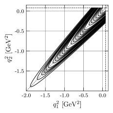
Figure 3: Range of photon virtualities spanned in our calculation on the ensembles cB211.072.64 (left), cC211.060.80 (middle), and cD211.054.96 (right). Dotted lines at $q_{1,2}^{2}=4m_{\pi}^{2}$ indicate the nonanalytic threshold beyond which the rotation to Euclidean spacetime is no longer valid.

The pion momentum $\vec{p}$ is set through the pseudoscalar interpolating operator while the momentum $\vec{q}_{1}$ is set through the current $j_{\mu}$, as shown in Eq. (6), with both momenta selected from the available finite-volume momenta $\vec{q}_{1},\vec{p}=2\pi/L\cdot\vec{n}$, where $\vec{n}\in\mathbb{Z}^{3}$. Momentum conservation sets the momentum $\vec{q}_{2}=\vec{p}-\vec{q}_{1}$. The energy $E_{\pi}$ of the pion is then imposed by the on-shell condition, while the temporal component $\omega_{1}$ of $q_{1}$ can be continuously varied as indicated in Eq. (5), with the temporal component $\omega_{2}$ of $q_{2}$ fixed by energy conservation to $\omega_{2}=E_{\pi}-\omega_{1}$. The kinematical range accessible on the lattice can be parameterized by the accessible virtualities of the electromagnetic currents,

$$q_{1}^{2} =\omega_{1}^{2}-\vec{q}_{1}^{\,2},$$

$$q_{2}^{2} =(E_{\pi}-\omega_{1})^{2}-(\vec{p}-\vec{q}_{1})^{2}.$$ (21)

For the Wick rotation to the Euclidean metric to be valid, the virtualities must fall below the two-pion threshold, i.e., $q_{i}^{2}<4m_{\pi}^{2}$.

For a pion at rest, $\vec{p}=0$, it holds that $E_{\pi}=m_{\pi}$ and $\vec{q}_{2}=-\vec{q}_{1}$. In this case, the photon virtualities simplify to

$$q_{1}^{2} =\omega_{1}^{2}-\vec{q}_{1}^{\,2},$$

$$q_{2}^{2} =(m_{\pi}-\omega_{1})^{2}-\vec{q}_{1}^{2}.$$ (22)

The analyticity constraint becomes a constraint on $\omega_{1}$,

$$\sqrt{4m_{\pi}^{2}+\vec{q}_{1}^{2}}+m_{\pi}<\omega_{1}<\sqrt{4m_{\pi}^{2}+\vec{q}_{1}^{2}}.$$ (23)

FIG. 3 depicts the kinematical range for 26 different choices of $|\vec{q}_{1}|^{2}$ satisfying $(2\pi/L)^{2}\leq|\vec{q}_{1}|^{2}\leq 32(2\pi/L)^{2}$ for each of the finite volumes accessible on the three distinct ensembles given in Tab. 1. For all three ensembles, the maximum momentum used in the evaluation of the three-point correlation function gives access to virtualities up to $|q_{1,2}^{2}|\approx 1.7\,\text{GeV}^{2}$.

Using Eqs. (1), (5) and (II.4) it is straightforward to show that in the rest frame of the pion $\tilde{A}_{\mu\nu}(\tau)$ vanishes when one or both Lorentz indices are temporal, while the spatial components can be written as

$$\tilde{A}_{ij}(\tau)=-im_{\pi}\epsilon_{ijk}q_{1}^{k}\tilde{A}(\tau).$$ (24)

Inverting the relation gives

$$\tilde{A}(\tau)=i\epsilon_{ijk}\frac{q_{1}^{k}}{m_{\pi}\vec{q}_{1}^{\,2}}\tilde{A}_{ij}(\tau),$$ (25)

where $\tilde{A}(\tau)$ is a scalar under the spatial rotation group. Combining Eqs. (1), (5) and (25) shows that the form factor can be extracted from a Laplace transform of this scalar quantity as

$$\mathcal{F}_{\pi^{0}\gamma\gamma}(q_{1}^{2},q_{2}^{2})=\int_{-\infty}^{\infty}d\tau\,\tilde{A}(\tau)e^{\omega_{1}\tau}.$$ (26)

Since the full TFF can be extracted from the scalar $\tilde{A}(\tau)$ in the rest frame of the pion, we focus on the evaluation of this scalar function for the remainder of this work.

The scalar amplitude $\tilde{A}(\tau)$ is implicitly parameterized by the momentum $\vec{q}_{1}$. All choices of momenta with a fixed value of $|\vec{q}_{1}|^{2}$ can be used to evaluate the form factor as in Eq. (26) at identical kinematics. We therefore choose to average the scalar amplitude over such equivalent momenta to increase statistics.

II.5 Finite-time extent corrections

All ensembles in this work use periodic (anti-periodic) temporal boundaries for the fundamental bosons (fermions). As a result, the pion experiences a periodic boundary condition in time, and the three-point function $C_{\mu\nu}$ receives corrections from states propagating backwards around the finite-time extent of our lattices. Denoting the lattice time extent $T$, including the leading correction gives

$$C_{\mu\nu}(\tau,t_{\pi}) \approx e^{-E_{\pi}t_{\pi}}\frac{Z_{\pi}}{2E_{\pi}}\left<0\left|T\{j_{\mu}(\tau)j_{\nu}(0)\}\right|\pi^{0}(\vec{p})\right>$$ (27)

$$+e^{-E_{\pi}(T-t_{\pi})}\frac{Z_{\pi}}{2E_{\pi}}\left<\pi^{0}(\vec{p})\left|T\{j_{\mu}(\tau)j_{\nu}(0)\}\right|0\right>$$

$$+O(e^{-\Delta Et_{\mathrm{sep}}}+e^{-\Delta E(T-|\tau|-t_{\mathrm{sep}})}).$$

In the rest frame of the pion, we can apply Bose symmetry and PT symmetry to define a corrected scalar amplitude $\tilde{A}(\tau)$ (cf. Eq. (25)) to account for this leading-order effect,

$$\tilde{A}(\tau;t_{\pi}) \equiv i\epsilon_{ijk}\frac{q_{1}^{k}}{m_{\pi}\vec{q}_{1}^{2}}\left[1-e^{E_{\pi}(T-|\tau|-t_{\pi})}\right]^{-1}\tilde{A}_{ij}(\tau;t_{\pi})$$ (28)

$$=\tilde{A}(\tau)+O(e^{-\Delta Et_{\mathrm{sep}}}+e^{-\Delta E(T-|\tau|-t_{\mathrm{sep}})}).$$

In all further analysis, this corrected form of the lattice amplitude is used as input.

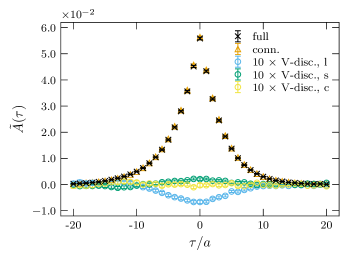
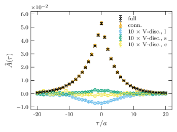
Figure 4: $\tilde{A}(\tau)$ with $|\vec{q}_{1}|^{2}=10(2\pi/L)^{2}$ including finite-time extent corrections on the ensembles cC211.060.80 (left) and cD211.054.96 (right). We show the full $\tilde{A}(\tau)$ as black crosses, the connected contribution as orange triangles, and the V-disconnected contributions (multiplied by 10 for easier comparison) with a light, strange and charm vector-current loop as blue, green and yellow circles, respectively.

II.6 Dependence on $t_{\pi}$

An example of the scalar amplitude $\tilde{A}(\tau)$ with the decomposition into contributions from individual Wick contractions is given in FIG. 4. These results, along with those used in the following analysis are based on the choice of interpolating operator time $t_{\pi}=2.23\,$fm for ensemble cB211.072.64, $t_{\pi}=2.18$ fm for ensemble cC211.060.80, and $t_{\pi}=2.28$ fm for ensemble cD211.054.96, with the choices made such that $t_{\pi}$ in physical units is similar on all three ensembles. Note that smaller values of $t_{\pi}$ lead to a reduction of the statistical errors, however, this requires a careful analysis of excited state effects. To confirm that our choices do not suffer from significant excited state effects, two larger choices of $t_{\pi}$ were measured on cB211.072.64 and cC211.060.80 and one larger choice on cD211.054.96. We depict an example of the comparison of $\tilde{A}(\tau;t_{\pi})$ across different choices of $t_{\pi}$ in FIG. 5. In all cases, $\tilde{A}(\tau;t_{\pi})$ does not show any systematic dependence on $t_{\pi}$ across the choices.

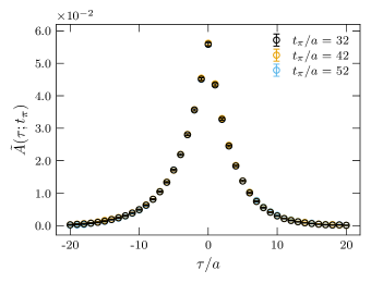
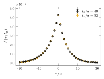
Figure 5: $\tilde{A}(\tau;t_{\pi})$ with $|\vec{q}_{1}|^{2}=10(2\pi/L)^{2}$ including finite-time extent corrections on the ensembles cC211.060.80 (left) and cD211.054.96 (right) for the choices $t_{\pi}\in\{2.18,2.86,3.55\}\,$fm (left) and $t_{\pi}\in\{2.28,3.02\}\,$fm (right).

II.7 Tail Fits

The extraction of the transition form factor using Eq. (5) in principle requires access to $\tilde{A}(\tau)$ for arbitrary $\tau\in(-\infty,\infty)$. To estimate the amplitude over the whole temporal range from our lattice data with finite temporal extent, we use two phenomenological models, the Vector Meson Dominance model (VMD) and Lowest Meson Dominance model (LMD) PhysRevD.94.053006 ; PhysRevD.51.4939 ; PhysRevLett.83.5230 . The VMD and LMD form factors are given, respectively, by

$$\mathcal{F}_{\pi^{0}\gamma\gamma}^{\mathrm{VMD}}(q_{1}^{2},q_{2}^{2})=\frac{\alpha M_{V}^{4}}{(M_{V}^{2}-q_{1}^{2})(M_{V}^{2}-q_{2}^{2})}$$ (29)

and

$$\mathcal{F}_{\pi^{0}\gamma\gamma}^{\mathrm{LMD}}(q_{1}^{2},q_{2}^{2})=\frac{\alpha M_{V}^{4}+\beta(q_{1}^{2}+q_{2}^{2})}{(M_{V}^{2}-q_{1}^{2})(M_{V}^{2}-q_{2}^{2})}.$$ (30)

The phenomenological origin of the models suggests particular parameter choices. In the chiral limit and at low energy, the fermionic triangle diagram gives rise to the Adler-Bell-Jackiw (ABJ) anomaly PhysRev.177.2426 ; BellJackiw , which constrains the form factor in these limits to

$$\mathcal{F}_{\pi^{0}\gamma\gamma}(0,0)=\frac{1}{4\pi^{2}F_{\pi}},$$ (31)

with $F_{\pi}=92.3(1)$ MeV the pion decay constant Workman:2022ynf , suggesting $\alpha=1/(4\pi^{2}F_{\pi})=0.274\,\mathrm{GeV}^{-1}$. Meanwhile, the mass $M_{V}=775\,\mathrm{MeV}$ is the $\rho$-meson mass in the VMD and LMD models, and $\beta=-F_{\pi}/3=-0.0308\,\mathrm{GeV}$ reproduces the leading OPE prediction PhysRevD.51.4939 ; PhysRevLett.83.5230 ; Gerardin:2016cqj . However, we treat $\alpha,M_{V}$ and $\beta$ as free model parameters when fitting the models to our data, using the models as inspiration for the fit form rather than a prediction of the precise asymptotic behavior.

Using the relation between the TFF and amplitude in Eq. (1) and inverting the relation in Eq. (5), the VMD and LMD form factors can be converted into fit functions for the Euclidean-time amplitude $\tilde{A}$ as follows. For the LMD fit function one finds

$$\tilde{A}^{\mathrm{LMD}}(\tau) =e^{m_{\pi}|\tau|\Theta(-\tau)}[C_{+}e^{-E_{V}|\tau|}-C_{-}e^{-(m_{\pi}+E_{V})|\tau|}],$$ (32)

in terms of

$$C_{\pm} \equiv\frac{\alpha M_{V}^{4}+\beta(2M_{V}^{2}+m_{\pi}^{2}\mp 2m_{\pi}E_{V})}{m_{\pi}E_{V}(2E_{V}\mp m_{\pi})},$$ (33)

$$E_{V} \equiv\sqrt{M_{V}^{2}+|\vec{q}_{1}|^{2}}.$$

The VMD fit function is obtained by setting $\beta=0$.

The VMD and LMD models should not be expected to fully capture the large-$Q^{2}$ behavior of the form factor, or conversely the small-$|\tau|$ behavior of $\tilde{A}(\tau)$. In particular, the Brodsky-Lepage behavior constrains the single-virtual form factor at large Euclidean (space-like) momentum Lepage:1979zb ; Lepage:1980fj ; Brodsky:1981rp , giving

$$\mathcal{F}_{\pi^{0}\gamma\gamma}(-Q^{2},0)\overset{Q^{2}\rightarrow\infty}{\longrightarrow}\frac{2F_{\pi}}{Q^{2}}$$ (34)

at leading order in $\alpha_{s}$. This behavior is reproduced by the VMD model, but the LMD model tends to a constant at large Euclidean momenta in the single-virtual form factor. Meanwhile, the operator product expansion (OPE) at short distances Nesterenko:1982dn ; Novikov:1983jt restricts the double-virtual form factor where both momenta become large at the same time, giving in the chiral limit

$$\mathcal{F}_{\pi^{0}\gamma\gamma}(-Q^{2},-Q^{2})\overset{Q^{2}\rightarrow\infty}{\longrightarrow}\frac{2F_{\pi}}{3}\left[\frac{1}{Q^{2}}+\mathcal{O}\left(\frac{1}{Q^{4}}\right)\right].$$ (35)

This behavior is reproduced by the LMD model (with the choice of $\beta$ given above), but the VMD model in this case falls off as $1/Q^{4}$ Gerardin:2016cqj . Despite these shortcomings at large $Q^{2}$, both models accurately capture the long-distance behavior. As such, we use the lattice data directly for the short-distance region while replacing only the tails with these fits. Details of this procedure are discussed in the following section.

III Transition Form Factor

To obtain the transition form factors, we need to evaluate the Laplace transform in Eq. (26), reproduced here for convenience:

$$\mathcal{F}_{\pi^{0}\gamma\gamma}(q_{1}^{2},q_{2}^{2})=\int_{-\infty}^{\infty}d\tau\,\tilde{A}(\tau)e^{\omega_{1}\tau},$$ (36)

where for a given momentum orbit $|\vec{q}_{1}|^{2}$ the squared four-momenta $q_{1}^{2}$ and $q_{2}^{2}$ are given by Eq. (II.4). The TFF is only directly available on specific sets of orbits $q_{1,2}^{2}$ determined by the kinematics, and it must therefore be interpolated/extrapolated to other points in the $(q_{1}^{2},q_{2}^{2})$ plane. In the following we describe our strategy for the numerical integration in Eq. (36) and for the extension of the TFF lattice data to the whole momentum plane using the modified $z$-expansion.

III.1 Numerical integration

The tails of $\tilde{A}(\tau)$ associated with large $|\tau|$ are expected to decrease exponentially quickly, with a mass scale predicted by the VMD/LMD models to be $E_{V}=\sqrt{M_{V}^{2}+|\vec{q}_{1}|^{2}}$ in one tail and $E_{V}+m_{\pi}$ in the other (see Eq. (32)). However, the exponential factor $e^{\omega_{1}\tau}$ enhances one tail of $\tilde{A}(\tau)$ significantly whenever $|\omega_{1}|$ is sufficiently large compared to this energy scale. This makes the numerical integration difficult: Since the signal-to-noise ratio decreases when going to larger $|\tau|$, fluctuations in one of the tails due to the small signal-to-noise ratio are exponentially enhanced. We observe that this effect is small for virtualities near the diagonal $q_{1}^{2}=q_{2}^{2}$, for which $\omega_{1}=m_{\pi}/2\ll E_{V}$, but can be severe in the single-virtual cases corresponding to either $q_{1}^{2}=0$ or $q_{2}^{2}=0$, for which $\omega_{1}=|\vec{q}_{1}|\approx E_{V}$, especially for the larger momentum orbits. FIG. 6

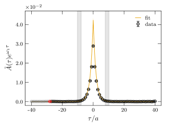
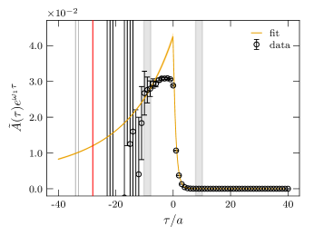
Figure 6: Integrands $\tilde{A}(\tau)e^{\omega_{1}\tau}$ with $|\vec{q}_{1}|^{2}=6(2\pi/L)^{2}$ on the ensemble cB211.072.64, comparing diagonal kinematics $q_{1}^{2}=q_{2}^{2}$ (left) and single-virtual kinematics $q_{2}^{2}=0$ (right). We show the integrand from lattice data as black circles and from a correlated LMD fit to $\tilde{A}(\tau)$ according to Eq. (32) as an orange line. The fit was done globally including all momentum orbits $(2\pi/L)^{2}\leq|\vec{q}_{1}|^{2}\leq 32(2\pi/L)^{2}$ with fit range $[-10,-8]\cup[8,10]$, indicated by the grey bands, yielding $\chi^{2}/\mathrm{d.o.f.}=1.01$ with correlations taken into account across all orbits and fit range. The red data point indicates the timeslice where the pseudoscalar operator is inserted, while the greyed-out points are those where the time ordering does not satisfy the one from Eq. (4).

shows a representative comparison of the integrand of the Laplace transform for both the diagonal and single-virtual cases. For choices of virtualities between these two cases, the exponential enhancement gets more and more pronounced when going from the diagonal to the single-virtual case.

These issues are addressed by the introduction of cutoff times $\tau^{R}_{\mathrm{cut}}$ and $\tau^{L}_{\mathrm{cut}}$, with lattice data replaced by a global fit to $\tilde{A}(\tau)$ for $\tau\geq\tau^{R}_{\mathrm{cut}}$ and $\tau\leq\tau^{L}_{\mathrm{cut}}$. In our analysis, we perform a fit to Eq. (32) across data at all available $\vec{q}_{1}$ and for values of $\tau$ selected from symmetrical fit ranges on both sides of the peak, i.e., $\tau\in[-\tau_{\mathrm{max}},-\tau_{\mathrm{min}}]\cup[\tau_{\mathrm{min}},\tau_{\mathrm{max}}]$. Variation of the fit ranges allows us to determine a corresponding systematic error. The left and right cutoff times are selected depending on the sign of $\omega_{1}$ to include as much data as possible on the exponentially suppressed tail of the integrand, in particular by fixing $\tau^{L}_{\mathrm{cut}}=-T/2$ for $\omega_{1}\geq 0$ or $\tau^{R}_{\mathrm{cut}}=T/2$ for $\omega_{1}<0$. The choice of the cutoff time $\tau_{\mathrm{cut}}$ is varied to assess the systematic error associated with this choice.

Finally, we filter the choices of cutoff times and kinematics to demand that for a given momentum orbit and value of $\omega_{1}$ a minimum percentage of $\mathcal{F}_{\pi^{0}\gamma\gamma}(q_{1}^{2},q_{2}^{2})$ must come from the lattice data. This is done to minimize the introduction of a model dependence in the final result. To do so, we define the data content for a given momentum and value of $\omega_{1}$ to be

$$\Delta_{\mathrm{latt.}}=\frac{\int_{\tau^{L}_{\textrm{cut}}}^{\tau^{R}_{\textrm{cut}}}d\tau\,\tilde{A}^{\textrm{(latt.)}}(\tau)e^{\omega_{1}\tau}}{\mathcal{F}_{\pi^{0}\gamma\gamma}(q_{1}^{2},q_{2}^{2})}.$$ (37)

In this work, we always restrict kinematics to only include TFFs for which $\Delta_{\mathrm{latt.}}\geq 95\%$.

III.2 Sampling in the Momentum Plane

As illustrated in FIG. 3, the transition form factor obtained from the lattice is a continuous function of $\omega_{1}$ for each spatial momentum orbit $|\vec{q}_{1}|^{2}$. In order to interpolate/extrapolate to the rest of the $(q_{1}^{2},q_{2}^{2})$ plane, we first sample choices of $\omega_{1}$ on which to evaluate the TFF as the input points for the fit. In this work, we do so by selecting $\omega_{1}$ corresponding to fixed choices of the ratio $q_{2}^{2}/q_{1}^{2}$, i.e., by finding the intersection between the available orbits and several diagonal “cuts” through the $(q_{1}^{2},q_{2}^{2})$ plane. Because the underlying lattice data are the same for all choices of $\omega_{1}$ within each orbit, data at nearby values of $\omega_{1}$ are strongly correlated. A relatively sparse sampling is therefore possible without sacrificing useful inputs to the $z$-expansion fits. Both $q_{2}^{2}/q_{1}^{2}=0$ and $q_{2}^{2}/q_{1}^{2}=1$ are useful choices of ratios to include, the former since the single-virtual transition form factor plays an important role in the evaluation of $a_{\mu}^{\pi^{0}-\mathrm{pole}}$, and the latter since we get the best signal-to-noise ratio in the transition form factor there.

We use the following procedure for the sampling in the momentum plane. We determine five values of $\omega_{1}$ on the highest momentum orbit $|\vec{q}_{1}|^{2}=32(2\pi/L)^{2}$, including those corresponding to the diagonal and single-virtual kinematics, such that the arc length of the curve parameterized by $\omega_{1}$ between neighbouring samples is constant. This fixes five ratios $q_{2}^{2}/q_{1}^{2}$ which are then used to determine the $\omega_{1}$ on all other spatial momentum orbits. To better cover the region close to single-virtual kinematics, we additionally include a cut $q_{2}^{2}/q_{1}^{2}=0.1$, as depicted in FIG. 7. We use several subsets of these cuts in the further analysis in order to determine systematic uncertainties associated with the sampling: all combinations of three cuts including both $q_{2}^{2}/q_{1}^{2}\in\{1,0\}$ and one of $q_{2}^{2}/q_{1}^{2}\in\{0.88,0.78,0.59,0.1\}$, and in addition a subset containing the four cuts $q_{2}^{2}/q_{1}^{2}\in\{1.0,0.88,0.1,0.0\}$. Including more than four cuts usually leads to an ill-conditioned covariance matrix yielding nonconverging or unstable fits.

For each cut, we impose a threshold for a minimal data content $\Delta_{\mathrm{latt.}}\geq 95\%$ (see Sec. III.1) in the TFF evaluated at each sampled kinematical point, dropping those from further analysis that do not meet the threshold.

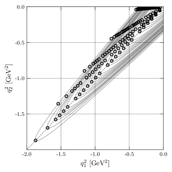
Figure 7: Cuts $(q_{2}^{2}/q_{1}^{2})\in\{1.0,0.88,0.78,0.59,0.1,0.0\}$ on ensemble cB211.072.64 illustrating our sampling of $\mathcal{F}_{\pi^{0}\gamma\gamma}(q_{1}^{2},q_{2}^{2})$ in the momentum plane used as input for the fit of the modified $z$-expansion.

III.3 $z$-Expansion

We use the modified $z$-expansion proposed in Gerardin:2019vio to interpolate/extrapolate the data from the sampling as described above to the whole kinematical range. This is a model-independent way of extending the transition form factor to arbitrary photon momenta which is preconditioned to more easily reproduce the form factor structure. Following Ref. Gerardin:2019vio , the model-independent fit form is constructed by first defining the conformal variables $z_{1}$ and $z_{2}$ as Boyd:1995sq

$$z_{k}=\frac{\sqrt{t_{c}+Q_{k}^{2}}-\sqrt{t_{c}-t_{0}}}{\sqrt{t_{c}+Q_{k}^{2}}+\sqrt{t_{c}-t_{0}}},\quad k\in\{1,2\},$$ (38)

where $Q_{k}^{2}=-q_{k}^{2}$ and $t_{c}=4m_{\pi}^{2}$ indicates the position of the branch cut due to the two-pion threshold. The parameter $t_{0}$ can be freely tuned to optimize the rate of convergence. For a given choice of $Q_{\mathrm{max}}^{2}$, to best map the region $0\leq Q_{1,2}^{2}\leq Q_{\mathrm{max}}^{2}$ to conformal variables near the origin, the optimal choice of $t_{0}$ is

$$t_{0}=t_{c}\left(1-\sqrt{1+Q_{\mathrm{max}}^{2}/t_{c}}\right),$$ (39)

which minimizes the maximum value of $|z_{k}|$ in the range $[0,Q_{\mathrm{max}}^{2}]$. We use $Q_{\mathrm{max}}^{2}=4$ GeV² in the present study, as this is the region yielding the dominant contribution to the integral for $a_{\mu}$ (see Sec. IV.1).

In terms of these conformal variables, one can expand

$$\mathcal{F}_{\pi^{0}\gamma\gamma}(-Q_{1}^{2},-Q_{2}^{2})=\sum_{n,m=0}^{\infty}c_{nm}z_{1}^{n}z_{2}^{m},$$ (40)

which is a convergent expansion within the analytic domain $|z_{k}|<1$. The coefficients $c_{nm}=c_{mn}$ are symmetric due to the Bose symmetry. By restricting the sum to $m,n\leq N$, one can approximate the form factor with accuracy determined by the choice of maximum order $N$. In addition, the transition form factor can be multiplied by an arbitrary analytic function $P(Q_{1}^{2},Q_{2}^{2})$ before expanding the resulting product in powers of $z_{k}$ as above. This preconditioning allows the expansion to more easily reproduce the form factor structure. As shown in Ref. Gerardin:2019vio , the choice

$$P(Q_{1}^{2},Q_{2}^{2})=1+\frac{Q_{1}^{2}+Q_{2}^{2}}{M_{V}^{2}},$$ (41)

where $M_{V}\approx 775\,\mathrm{MeV}$ is the $\rho$-meson mass, leads to a parameterization of the transition form factor which decreases asymptotically as $1/Q^{2}$ in all directions in the momentum plane even at finite values of $N$, thus satisfying the momentum dependence of Eqs. (34) and (35). As shown in Ref. Bourrely:2008za , to enforce the appropriate scaling at the two-pion threshold, the expansion should be further modified to fix the derivatives of the transition form factors with respect to $z_{k}$ at $z_{k}=-1$ to zero. Including the cutoff $N$, preconditioning, and threshold constraints gives the modified expansion Gerardin:2019vio

$$P(Q_{1}^{2},Q_{2}^{2})\mathcal{F}_{\pi^{0}\gamma\gamma}(-Q_{1}^{2}, -Q_{2}^{2})$$

$$\approx\sum_{m,n=0}^{N}c_{nm} \left(z_{1}^{n}-(-1)^{N+n+1}\frac{n}{N+1}z_{1}^{N+1}\right)$$

$$\times \left(z_{2}^{m}-(-1)^{N+m+1}\frac{m}{N+1}z_{2}^{N+1}\right).$$ (42)

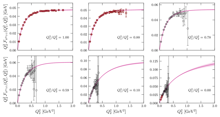
Figure 8: Correlated $z$-expansion fit to the TFFs evaluated on ensemble cC211.060.80 using $c_{00},c_{10},c_{11}$ and $c_{22}$. Shown is $Q_{2}^{2}\,\mathcal{F}_{\pi^{0}\gamma\gamma}(Q_{1}^{2},Q_{2}^{2})$, plots showing $\mathcal{F}_{\pi^{0}\gamma\gamma}(Q_{1}^{2},Q_{2}^{2})$ can be found in FIG. 9. Only TFF data points with at least 95% data content are included (colored in red for the used cuts $(q_{2}^{2}/q_{1}^{2})\in\{1.0,0.88,0.0\}$); data in grey with less than 95% data content are shown for illustration only. For $\tilde{A}(\tau)$ a global LMD fit with fit range $[20,21]$ and $\tau_{\mathrm{cut}}=23$ in lattice units is used. The reduced $\chi^{2}$ are $\chi^{2}_{\tilde{A}}/\mathrm{d.o.f.}=0.86$ and $\chi^{2}_{z\mathrm{-exp.}}/\mathrm{d.o.f.}=1.00$.

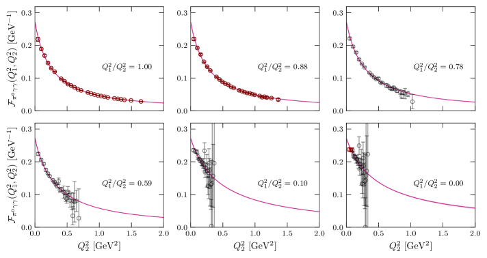
Figure 9: Same as FIG. 8, but showing $\mathcal{F}_{\pi^{0}\gamma\gamma}(Q_{1}^{2},Q_{2}^{2})$ instead of $Q_{2}^{2}\mathcal{F}_{\pi^{0}\gamma\gamma}(Q_{1}^{2},Q_{2}^{2})$ in order to highlight the quality of fit at low values of $Q_{2}^{2}$.

In the following, we either fit the coefficients $c_{nm}$ independently to the data for each ensemble or perform a combined fit to all three ensembles with correction terms for $\mathcal{O}(a^{2})$ lattice artifacts as

$$c_{nm}(a)=c_{nm}(0)+\delta_{nm}\left(\frac{a}{a_{\mathrm{ref.}}}\right)^{2},$$ (43)

where we use the cC211.060.80 lattice spacing for $a_{\mathrm{ref.}}$, i.e., $a_{\mathrm{ref.}}=0.06821(12)\,$fm. The continuum-extrapolation strategies based on these two options are considered below in Sec. VI.

In contrast to Refs. Gerardin:2019vio and Ref. Gerardin:2023naa we perform fully correlated fits with the modified $z$-expansion. We use $N=1,2$ and all possible combinations of the $N=1$ coefficients with one of the $N=2$ coefficients. We find that the resulting fits describe the lattice data well, even along the cuts not included in the fit, as seen in the example in FIG. 8 and 9.

Note that the transition form factors obtained from Eq. (42) multiplied by $Q^{2}$ asymptote to a constant by construction, with predictions for the single-virtual and diagonal case described in Eqs. (34) and (35), respectively. We exclude analyses in which the single-virtual transition form factor multiplied by $Q^{2}$ turn out to be asymptotically negative, since this clearly violates those predictions.

We find that correlated $z$-expansion fits with cutoffs set to either $N=1$ or $N=2$ already lead to a good quality of fit when including input data from three or four cuts in the momentum plane as described in Sec. III.2. For $N=2$, at least two of the coefficients $c_{nm}$ are strongly correlated, indicating a degeneracy in the parameterization. Even when including only one of the second-order coefficients in conjunction with all three first-order coefficients, we find slight correlations between some of them. See FIG. 10 for a corner plot depicting correlations in a representative case when including coefficients $\{c_{00},c_{10},c_{11},c_{22}\}$.

The corresponding correlation matrix is given by

$$\mathrm{cor}(c_{nm})=\left(\begin{array}[]{cccc}+1.00&-0.30&-0.39&+0.31\\ -0.30&+1.00&-0.05&-0.14\\ -0.39&-0.05&+1.00&-0.88\\ +0.31&-0.14&-0.88&+1.00\end{array}\right),$$ (44)

clearly showing the strong (anti)correlation between $c_{11}$ and $c_{22}$, and lesser (anti)correlations between all other coefficients except for $c_{10}$ and $c_{11}$ which are almost completely uncorrelated. When including all $N=2$ coefficients, it turns out that $c_{20}$ and $c_{21}$ are strongly correlated with $c_{11}$ for almost all choices of parameters. To get reliable estimates of the individual coefficients, it is desirable to remove such near-degeneracies in the parameterization by only using a subset of the coefficients which are not strongly correlated. In the final analysis, we therefore determine the preferred values of all quantities studied based on a $z$-expansion parameterization with minimal degeneracy, but we use variations between these choices of parameterizations to determine an additional systematic error.

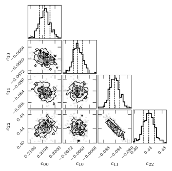
Figure 10: Corner plot for the coefficients $c_{00},c_{10},c_{11}$ and $c_{22}$ from the correlated $z$-expansion fit to the TFFs on cC211.060.80 as shown in FIG. 8 and 9 from a jackknife resampling. The corresponding correlation matrix is given in Eq. (44).

IV Observables

The main observable studied in this work is $a_{\mu}^{\pi^{0}-\mathrm{pole}}$, i.e., the pion-pole contribution to the muon $(g-2)/2$. We further study the two-photon decay width $\Gamma(\pi\to\gamma\gamma)$ and the slope parameter $b_{\pi}$, both of which are related to $\mathcal{F}_{\pi^{0}\gamma\gamma}$.

IV.1 Pion-pole contribution to $a_{\mu}$

Following Refs. PhysRevD.94.053006  and Jegerlehner2009 , we use the three-dimensional integral representation for the pion-pole contribution

$$a_{\mu}^{\pi^{0}-\mathrm{pole}} =\left(\frac{\alpha}{\pi}\right)^{3}\left[a_{\mu}^{\pi^{0}-\mathrm{pole}(1)}+a_{\mu}^{\pi^{0}-\mathrm{pole}(2)}\right],$$ (45)

where $\alpha$ is the fine structure constant,

$$a_{\mu}^{\pi^{0}-\mathrm{pole}(1)} =\int_{0}^{\infty}dQ_{1}\int_{0}^{\infty}dQ_{2}\int_{-1}^{1}d\tau\,$$ (46)

$$w_{1}(Q_{1},Q_{2},\tau)\mathcal{F}_{\pi^{0}\gamma\gamma}(-Q_{1}^{2},-Q_{3}^{2})\mathcal{F}_{\pi^{0}\gamma\gamma}(-Q_{2}^{2},0),$$

and

$$a_{\mu}^{\pi^{0}-\mathrm{pole}(2)} =\int_{0}^{\infty}dQ_{1}\int_{0}^{\infty}dQ_{2}\int_{-1}^{1}d\tau\,$$ (47)

$$w_{2}(Q_{1},Q_{2},\tau)\mathcal{F}_{\pi^{0}\gamma\gamma}(-Q_{1}^{2},-Q_{2}^{2})\mathcal{F}_{\pi^{0}\gamma\gamma}(-Q_{3}^{2},0).$$

The integration is performed over the magnitudes $Q_{1}$, $Q_{2}$ of two of the four-momenta and $\tau=\cos\theta$ describing the angle $\theta$ between them, with the magnitude of the third four-momentum fixed by $Q_{3}^{2}=Q_{1}^{2}+Q_{2}^{2}+2Q_{1}Q_{2}\tau$. The weight functions $w_{1}$ and $w_{2}$ are given in Appendix A. Note that $w_{1,2}$ are both dimensionless and $w_{1,2}(Q_{1},Q_{2},\tau)\rightarrow 0$ for $Q_{1,2}\rightarrow 0$ and for $\tau\rightarrow\pm 1$. Further, $w_{2}$ is symmetric under the exchange of $Q_{1}$ and $Q_{2}$. In Ref. PhysRevD.94.053006 , the weight functions for the pion are studied and discussed in detail. One finds that the momentum region $Q_{1,2}\leq 0.5\,$GeV is the most important in Eqs. (46) and (47) for $a_{\mu}^{\pi^{0}-\mathrm{pole}}$, which is where we have the strongest data support from our lattice calculation. For two examples illustrating the concentration of the weight functions at low momenta, see FIG. 11. In particular, note that $w_{2}(Q_{1},Q_{2},\tau)$ is roughly an order of magnitude smaller than $w_{1}(Q_{1},Q_{2},\tau)$.

By introducing a momentum cutoff $\Lambda$, i.e., by replacing

$$\int_{0}^{\infty}dQ_{1,2}\;\longrightarrow\;\int_{0}^{\Lambda}dQ_{1,2}$$ (48)

in Eqs. (46) and (47), one can estimate the importance of various momentum regions in the evaluation of Eqs. (46) and (47). Though the cutoffs are only directly imposed on $Q_{1,2}$, they imply a cutoff of $Q_{3}\leq 2\Lambda$ on the third momentum as well. We find that the integrals saturate rapidly, such that we get around 85% of the total result with $\Lambda=1$ GeV and around 90% with $\Lambda=1.5$ GeV, i.e., from momentum regions with strong data support from our lattice calculation. An example of this exercise is shown in FIG. 12.

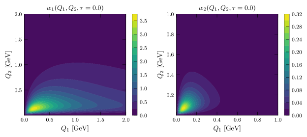
Figure 11: Weight function $w_{1}(Q_{1},Q_{2},\tau)$ (left) and $w_{2}(Q_{1},Q_{2},\tau)$ (right) for the pion for momenta $Q_{1}$ and $Q_{2}$ and $\tau=\cos\theta$ where $\theta=90^{\circ}$, showing the concentration at low momenta. Note the different momentum range for and magnitude of $w_{2}$ as well as its symmetry with respect to $Q_{1}\leftrightarrow Q_{2}$.

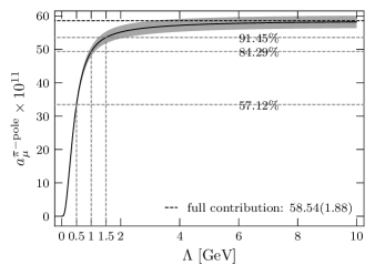
Figure 12: Contribution to $a_{\mu}^{\pi^{0}-\mathrm{pole}}$ for increasing cutoff $\Lambda$ for ensemble cC211.060.80, using a $N=2$ correlated $z$-expansion fit to $(q_{2}^{2}/q_{1}^{2})\in\{1.0,0.88,0.1,0.0\}$. Only TFF data points where at least 95% of the transition form factors come from lattice data are included, for $\tilde{A}(\tau)$ a global LMD fit with fit range $[7,8]$ and $\tau_{\mathrm{cut}}=26$ in lattice units is used. The reduced $\chi^{2}$ are $\chi^{2}_{\tilde{A}}/\mathrm{d.o.f.}=0.85$ and $\chi^{2}_{z~{}\mathrm{exp.}}/\mathrm{d.o.f.}=1.02$. Indicated is the saturation at $\Lambda\in\{0.5,1.0,1.5\}$ GeV as well as the value of the full contribution for this particular choice of parameters.

IV.2 Decay Width and Slope Parameter

To leading order in the fine structure constant $\alpha$, the transition form factors determine the partial decay width through

$$\Gamma(\pi\to\gamma\gamma)=\frac{\pi\alpha^{2}m_{\pi}^{3}}{4}\left|\mathcal{F}_{\pi^{0}\gamma\gamma}(0,0)\right|^{2}+O(\alpha^{3}).$$ (49)

The neutral-pion decay width has been measured in the PrimEx and PrimEx-II experiments PrimEx:2010fvg ; doi:10.1126/science.aay6641 with a combined result of $\Gamma(\pi\to\gamma\gamma)=7.802(52)_{\mathrm{stat}}(105)_{\mathrm{sys}}(117)_{\mathrm{tot}}$ eV. At our level of statistical precision, uncertainties from radiative corrections to the decay width are negligible and we therefore quote the leading-order result as our estimate of this quantity.

Further, the transition form factors can be used to extract the slope parameter

$$b_{\pi}=\frac{1}{\mathcal{F}_{\pi^{0}\gamma\gamma}(0,0)}\frac{\mathrm{d}\mathcal{F}_{\pi^{0}\gamma\gamma}(q^{2},0)}{\mathrm{d}q^{2}}\Bigg{|}_{q^{2}=0},$$ (50)

thus providing input for determining the electromagnetic interaction radius of the pion. The averaged experimental result for the slope parameter is $b_{\pi}=1.84(17)$ GeV^-2 Workman:2022ynf .

These quantities are easily extracted from the form of the $z$-expansion fit at $(q_{1}^{2},q_{2}^{2})=(0,0)$. The value of $\mathcal{F}_{\pi^{0}\gamma\gamma}(0,0)$ comes directly from the $z$-expansion fit, while the derivative can be acquired by differentiating the form of the $z$-expansion in Eq. (42) with respect to $-Q_{1}^{2}$, yielding the slope parameter

$$b_{\pi} =-\frac{d}{dQ_{1}^{2}}\ln\mathcal{F}_{\pi^{0}\gamma\gamma}(-Q_{1}^{2},0)\big{|}_{Q_{1}^{2}=0}$$ (51)

$$\approx\frac{1}{M_{V}^{2}}-\frac{1}{z_{1}}\frac{dz_{1}}{dQ_{1}^{2}}\Big{[}\sum_{\begin{subarray}{c}m=0\\ n=1\end{subarray}}^{N}nc_{nm}\left(z_{1}^{n}-(-1)^{N+n+1}z_{1}^{N+1}\right)$$

$$\hskip 55.0pt\times\left(z_{2}^{m}-(-1)^{N+m+1}\frac{m}{N+1}z_{2}^{N+1}\right)\Big{]}_{Q_{1,2}^{2}=0}.$$

The term in square brackets can be directly evaluated, and the derivative of the conformal parameter is given by

$$\frac{1}{z_{1}}\frac{dz_{1}}{dQ_{1}^{2}}\Bigg{|}_{Q_{1}^{2}=0}=\frac{1}{t_{0}}\sqrt{1-t_{0}/t_{c}}.$$ (52)

V Model averaging and error estimation

We follow different analysis chains from the initial lattice correlation function data to estimates of the quantities $a_{\mu}^{\pi^{0}-\mathrm{pole}}$, $\Gamma(\pi\to\gamma\gamma)$ and $b_{\pi}$. Each such chain is determined by a choice of parameters, namely the choice of fit range and fit model in the fit to $\tilde{A}(\tau)$, $\tau_{\mathrm{cut}}$ when constructing the transition form factors and finally the included cuts in the momentum plane in the fit to the modified $z$-expansion. This yields $\mathcal{O}(10^{3}-10^{4})$ estimates. For the remainder of this section such a choice of parameters is called an “analysis”. A priori, only fits with $\chi^{2}_{\tilde{A}}/\mathrm{d.o.f.}$ close to 1 are included in an analysis chain for the single ensemble analyses, with $0.84\lesssim\chi^{2}_{\tilde{A}}/\mathrm{d.o.f.}\lesssim 2.05$. For the combined $z$-expansion fits the input $\tilde{A}(\tau)$ fit ranges and $\tau_{\mathrm{cut}}$ were chosen to be similar in physical units across all ensembles, using $t_{min}\in[0.48,1.27]$ fm, $t_{max}\in[0.64,1.43]$ fm and $\tau_{\mathrm{cut}}\in[1.35,2.07]$ fm on cB211.072.64 as a reference and remaining within $10\%$ of these physical-units values for the cC211.060.80 and cD211.054.96 ensembles. The fits across all ensembles are of good quality, with $\chi^{2}$ values in the range $1\lesssim\chi^{2}_{\tilde{A}}/\mathrm{d.o.f.}\lesssim 2.4$ with an average of $\bar{\chi}^{2}_{\tilde{A}}/\mathrm{d.o.f.}\approx 1.5$.

We calculate the statistical errors for each analysis using the jackknife resampling procedure, finding that there is virtually no autocorrelation between the input data $\tilde{A}(\tau)$ amongst the available configurations listed in Tab. 1. Jackknife resampling is applied over the entire analysis pipeline for each set of analysis choices, ensuring that statistical errors are fully propagated.

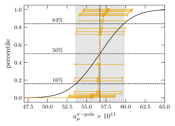
Figure 13: Cumulative distribution functions (CDF) of $a_{\mu}^{\pi^{0}-\mathrm{pole}}$ for the combined fit using $c_{nm}=\{c_{00},c_{10},c_{11},c_{22}\}$. The orange curve shows the CDF of $\approx$15’000 different analyses obtained from their AIC weights, the errors on the orange point show the statistical errors for some analyses with a significant weight in the model averaging. This curve corresponds to statistical errors rescaled by $\lambda=0$ while the black curve corresponds to rescaling by $\lambda=1$. The latter gives the central value by the $50\%$ percentile, and the total error as the half variation between the $16\%$ and $84\%$ percentiles shown in gray. To separate the statistical and systematic part of the error, we further calculate the error of the distribution with statistical errors rescaled by $\lambda=2$ (not shown in the figure), as described in the main text.

To take a weighted average of estimates under various analysis choices in an analysis chain, we use a modified version of the Akaike Information Criterion (AIC) Akaike1978 ; Jay2021 . Closely following the method introduced in doi:10.1126/science.1257050 and Borsanyi:2020mff , the model averaging proceeds as follows. For a target observable $y$, here $a_{\mu}^{\pi^{0}-\mathrm{pole}}$, $\Gamma(\pi\to\gamma\gamma)$ or $b_{\pi}$, we build a histogram from the different analyses, assigning to each analysis a weight given by the AIC. This criterion is derived from the Kullback-Leibler divergence, which measures the distance of a fit function from the true distribution of the points (for a derivation see Ref. doi:10.1126/science.1257050 ). We use the modified AIC introduced in Borsanyi:2020mff ,

$$\text{AIC}\sim\exp\left[-\frac{1}{2}\left(\chi^{2}+2n_{\text{par}}-n_{\text{data}}\right)\right],$$ (53)

where the $\chi^{2}$, the number of fit parameters $n_{\text{par}}$ and the number of data points $n_{\text{data}}$ describe the fit of interest. The first two terms in the exponent correspond to the standard AIC, and the last term is needed to weigh fits with different lengths in the fit ranges when fitting to $\tilde{A}(\tau)$ or to weight $z$-expansion fits with a differing number of cuts in the momentum plane when sampling the transition form factors.

In general, two fitting steps are involved in the determination of each of $a_{\mu}^{\pi^{0}-\mathrm{pole}}$, $\Gamma(\pi^{0}\to\gamma\gamma)$, and $b_{\pi}$ on a given ensemble: the global fit to $\tilde{A}(\tau)$ and the $z$-expansion fit to the transition form factors. A combined weight can be assigned to each combination of fitting choices across both of these steps by multiplying the respective AIC weights $\tilde{w}_{i}$ given in Eq. (53). In the alternative simultaneous continuum and $z$-expansion fit procedure described in Sec. III.3, the model averaging step is instead performed globally across all three ensembles, and therefore a combined AIC weight is assigned by multiplying the weights of the fits to $\tilde{A}(\tau)$ across all three ensembles as well as the weight of the final global $z$-expansion fit with lattice artifacts included. In either case, the result is one unnormalized weight $\tilde{w}_{i}$ per analysis.

Given the weights $\tilde{w}_{i}$, central values $m_{i}$, and statistical error $\sigma_{i}$ from each analysis, the global cumulative distribution function (CDF) is expected to be well-described by a weighted combination of normal distribution CDFs. We take the median of the CDF as the central value across all analyses and the half variation between the 16% and 84% percentiles as the total error. To separate statistical and systematic errors, the same procedure can be performed with errors rescaled as $\sigma_{i}\rightarrow\sqrt{\lambda}\sigma_{i}$. The variation between $\lambda=2$ and $\lambda=1$ yields a separate statistical and systematic error Borsanyi:2020mff . For an illustration, see FIG. 13.

For a better understanding on the composition of the systematic error, we follow the error budgeting procedure suggested in Borsanyi:2020mff : For each of the choices made during the analysis chain, e.g., the choice between the VMD or LMD fit to $\tilde{A}(\tau)$ or the different fit ranges, we first determine the total error for each possible option, varying all other components of the analysis. We then construct a second CDF as above with $m_{i}$ the average of the 16% and 84% percentiles, $\sigma_{i}$ the total error and $w_{i}$ the sum of the weights coming from this choice. Using this CDF, we derive the systematic error as described above for the original CDF; this is our result for the systematic error corresponding to the choice. Note that the estimated systematic errors associated with each of the steps of the analysis by this procedure are correlated, thus they do not sum up quadratically to the full systematic error.

VI Lattice results and continuum extrapolation

Here, our results using the model averaging described in Sec. V are summarized. Comparing to our earlier publication BurriPoS2022 we have refined the analysis by systematically studying different $z$-expansion fits and by excluding analyses leading to unphysical TFFs as described in Sec. III.3.

For the single ensemble analyses, we perform an AIC averaging over different fit models and fit ranges for $\tilde{A}(\tau)$, different choices of $\tau_{\mathrm{cut}}\approx[1.3,2.0]$ fm on all three ensembles, different samplings in the momentum plane and different choices of $z$-expansion fits. The results including error budgeting are summarized in Tab. 3, and are shown in FIG. 16 as diamonds (cD211.054.96), triangles (cC211.060.80), and circles (cB211.072.64), respectively. We note that the error budgets from fit model and fit range are very small, indicating that by restricting the transition form factors in the $z$-expansion to have at least a 95% contribution from lattice data effectively removes the dependence on the model used to fit the tails of $\tilde{A}(\tau)$ almost completely.

cB211.072.64	$a_{\mu}^{\pi^{0}-\mathrm{pole}}\times 10^{11}$	$\Gamma(\pi\to\gamma\gamma)$ [eV]	$b_{\pi}$ [GeV-2]
value	57.5(1.8)	6.89(0.33)	1.63(0.18)
$\sigma_{\mathrm{stat}}$	1.39	0.28	0.11
$\sigma_{\mathrm{sys}}$	1.16	0.18	0.15
fit model	0.09	0.01	0.01
fit range	0.00	0.00	0.00
$\tau_{\mathrm{cut}}$	0.17	0.06	0.03
sampling	0.20	0.06	0.04
$z$-exp.	1.15	0.17	0.14

cC211.060.80	$a_{\mu}^{\pi^{0}-\mathrm{pole}}\times 10^{11}$	$\Gamma(\pi\to\gamma\gamma)$ [eV]	$b_{\pi}$ [GeV-2]
value	56.7(2.0)	6.72(0.29)	1.54(0.14)
$\sigma_{\mathrm{stat}}$	1.33	0.28	0.13
$\sigma_{\mathrm{sys}}$	1.54	0.08	0.04
fit model	0.01	0.00	0.00
fit range	0.07	0.01	0.00
$\tau_{\mathrm{cut}}$	0.36	0.03	0.02
sampling	0.50	0.03	0.03
$z$-exp.	1.51	0.04	0.02

cD211.054.96	$a_{\mu}^{\pi^{0}-\mathrm{pole}}\times 10^{11}$	$\Gamma(\pi\to\gamma\gamma)$ [eV]	$b_{\pi}$ [GeV-2]
value	58.1(2.1)	7.51(0.39)	2.03(0.09)
$\sigma_{\mathrm{stat}}$	2.08	0.36	0.06
$\sigma_{\mathrm{sys}}$	0.37	0.13	0.06
fit model	0.00	0.00	0.00
fit range	0.01	0.00	0.00
$\tau_{\mathrm{cut}}$	0.19	0.08	0.03
sampling	0.10	0.05	0.03
$z$-exp.	0.29	0.10	0.06

Table 3: Values of measured observables on each ensemble, with systematic error budgeting indicated below each result.

For the $z$-expansion fits considered in the combined fitting, the set $c_{nm}=\{c_{00},c_{10},c_{11},c_{22}\}$ with the lattice-artefact correction coefficients $\delta_{nm}=\{\delta_{00},\delta_{10}\}$ leads to the least correlation amongst the coefficients and gives an AIC-averaged fully correlated $\chi^{2}/\mathrm{d.o.f.}=1.36$. The AIC-averaged $z$-expansion coefficients (cf. Eq. (42)) in the continuum limit based on the combined fit across all ensembles are given by

$c_{00}$	$c_{10}$	$c_{11}$	$c_{22}$
0.2220(48)	-0.0596(59)	-0.050(18)	0.27(14)

with correlation matrix

$$\mathrm{cor}(c_{nm})=\left(\begin{array}[]{cccc}+1.00&-0.46&-0.07&+0.07\\ -0.46&+1.00&+0.03&-0.08\\ -0.07&+0.03&+1.00&-0.83\\ +0.07&-0.08&-0.83&+1.00\end{array}\right)$$ (54)

and the corresponding corner plot given in FIG. 14.

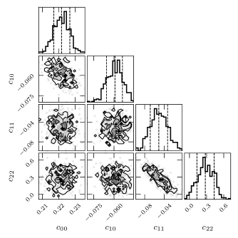
Figure 14: Corner plot of the AIC averaged coefficients of the combined correlated $z$-expansion fit, utilizing bootstrap resampling on each ensemble, where only the coefficients $c_{00},c_{10},c_{11}$ and $c_{22}$ were used. Notice the anticorrelation between $c_{11}$ and $c_{22}$ and the less severe anticorrelation between $c_{00}$ and $c_{10}$. All other coefficients are virtually uncorrelated. The corresponding correlation matrix is given in Eq. (69).

This is our preferred continuum result. We note that the coefficients describing the lattice artefacts are very small and compatible with zero, $\delta_{00}=0.0005(41)$ and $\delta_{10}=-0.0085(49)$. The resulting continuum TFFs for diagonal and single-virtual kinematics are shown in FIG. 15. The figure further indicates the kinematic region directly supported by lattice data, where the fit is expected to be most reliable. For the single-virtual kinematics we find good agreement with the CELLO CELLO:1990klc bins below $Q^{2}\lesssim 2\text{ GeV}^{2}$, while at larger momenta $Q^{2}\gtrsim 2\text{ GeV}^{2}$ our analysis results tend to be systematically lower than the experimental ones.

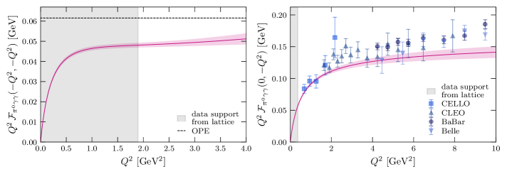
Figure 15: Transition form factor from the combined fit for diagonal (left) and single-virtual (right) kinematics. For the diagonal kinematics, the OPE prediction for large $Q^{2}$ is indicated by the horizontal dashed line while for the single-virtual kinematics, experimental values from CELLO CELLO:1990klc , CLEO CLEO:1997fho , BaBar BaBar:2009rrj ; BaBar:2011nrp and Belle Belle:Uehara2012 are shown. The region with direct support from lattice data is shaded in grey.

For the quantities $a_{\mu}^{\pi^{0}-\mathrm{pole}}$, $\Gamma(\pi\to\gamma\gamma)$ and $b_{\pi}$, in order to account for different choices of $z$-expansion parameters in a more conservative way than by using the AIC, we use a procedure inspired by the method described in Ref. ExtendedTwistedMass:2021gbo . It consists of taking the absolute difference of the central value of the combined fit using the coefficient set $c_{nm}=\{c_{00},c_{10},c_{11},c_{22}\}$ and the weighted average of the results from the other considered fits each weighted with $1/\sigma_{\mathrm{tot}}^{2}$ as an additional systematic error $\sigma_{\mathrm{sys,}\,z\mathrm{-exp.}}$ added in quadrature. We find

$$\begin{gathered}a_{\mu}^{\pi^{0}-\mathrm{pole}}=56.7(3.1)_{\mathrm{stat}}(1.0)_{\mathrm{sys}}[3.2]_{\mathrm{tot}}\times 10^{-11},\\ \Gamma(\pi\to\gamma\gamma)=7.50(0.48)_{\mathrm{stat}}(0.16)_{\mathrm{sys}}[0.50]_{\mathrm{tot}}\,\mathrm{eV},\\ b_{\pi}=2.16(0.07)_{\mathrm{stat}}(0.19)_{\mathrm{sys}}[0.20]_{\mathrm{tot}}\,\mathrm{GeV}^{-2}.\end{gathered}$$ (55)

These values including a detailed error budget are summarized in Tab. 4,

combined fit	$a_{\mu}^{\pi^{0}-\mathrm{pole}}\times 10^{11}$	$\Gamma(\pi\to\gamma\gamma)$ [eV]	$b_{\pi}$ [GeV-2]
value	56.7(3.2)	7.50(0.50)	2.16(0.20)
$\sigma_{\mathrm{stat}}$	3.06	0.48	0.07
$\sigma_{\mathrm{sys,}\,z\mathrm{-exp.}}$	0.91	0.14	0.19
$\sigma_{\mathrm{sys}}$	0.35	0.07	0.01
fit model	0.00	0.00	0.00
fit range	0.00	0.00	0.00
$\tau_{\mathrm{cut}}$	0.33	0.07	0.00
sampling	0.19	0.05	0.01

Table 4: Preferred continuum result from the combined fit using $c_{nm}=\{c_{00},c_{10},c_{11},c_{22}\}$ and $\delta_{nm}=\{\delta_{00},\delta_{10}\}$. $\sigma_{\mathrm{sys,}\,z\mathrm{-exp.}}$ denotes the more conservative systematic error from different $z$-expansion parameter choices as described in the text.

and are shown in FIG. 16 as crosses.

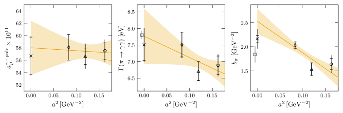
Figure 16: Combined fit and single ensemble results from Tabs. 3 and 4: $a_{\mu}^{\pi^{0}-\mathrm{pole}}$ (left), $\Gamma(\pi\to\gamma\gamma)$ (middle) and $b_{\pi}$ (right). Indicated are the statistical and total errors. For comparison, we also show linear fits in $a^{2}$ on the per-ensemble data points. In each plot, the points with caps on the errorbars correspond to the combined fit (cross), the cD211.054.96 (diamond), the cC211.060.80 (triangle) and the cB211.072.64 (circle) result. In the $\Gamma(\pi\to\gamma\gamma)$ and $b_{\pi}$ plots, the square symbols show the experimental values and their errors, namely $\Gamma(\pi\to\gamma\gamma)=7.802(117)$ eV doi:10.1126/science.aay6641 and $b_{\pi}=1.84(17)$ GeV^-2 Workman:2022ynf .

Instead of using the continuum values of the $z$-expansion coefficients from the combined fit to calculate the continuum values of $a_{\mu}^{\pi^{0}-\mathrm{pole}}$, $\Gamma(\pi\to\gamma\gamma)$ and $b_{\pi}$, we could also extrapolate their per-ensemble values in $a^{2}$ directly. As depicted in FIG. 16, we find that fits linear in $a^{2}$ agree well with the combined fit continuum results, albeit with significantly larger errors at $a^{2}=0$. We note that at the current level of accuracy the lattice artefacts in $a_{\mu}^{\pi^{0}-\mathrm{pole}}$ are compatible with zero. Hence, a continuum extrapolation with a constant is also possible leading to a better $\chi^{2}/\mathrm{d.o.f.}$ and a significantly smaller error. However, in order to be on the conservative side, we do not consider this value in our analysis.

Our result for $a_{\mu}^{\pi^{0}-\mathrm{pole}}$ is compatible with our earlier analysis BurriPoS2022 , where we used a continuum extrapolation in the individual ensemble estimates of each observable instead of one coming from a combined fit to the TFF across ensembles. It is also compatible with the recent lattice result $a_{\mu}^{\pi^{0}-\mathrm{pole}}=57.8\pm 1.8_{\mathrm{stat}}\pm 0.9_{\mathrm{sys}}\times 10^{-11}$ from the BMW collaboration in Ref. Gerardin:2023naa , and $a_{\mu}^{\pi^{0}-\mathrm{pole}}=59.7\pm 3.6\times 10^{-11}$ from the Mainz group in Ref. Gerardin:2019vio . Comparing to the dispersive result $a_{\mu}^{\pi^{0}-\mathrm{pole}}=63.0^{+2.7}_{-2.1}\cdot 10^{-11}$ from Refs. Aoyama:2020ynm ; Hoferichter:2018dmo ; Hoferichter:2018kwz , we find that our result is compatible at the level of 1.6 $\sigma$.

For $\Gamma(\pi\to\gamma\gamma)$, we again find agreement with $\Gamma(\pi\to\gamma\gamma)=7.11\pm 0.44_{\mathrm{stat}}\pm 0.21_{\mathrm{sys}}$ GeV^-2 from Ref. Gerardin:2023naa . Our result is also compatible with the experimental value $\Gamma(\pi\to\gamma\gamma)=7.802(52)_{\mathrm{stat}}(105)_{\mathrm{sys}}$ eV from Ref. doi:10.1126/science.aay6641 .

Finally, for $b_{\pi}$, our result is compatible with the experimental result $b_{\pi}=1.84(17)$ GeV^-2 from Ref. Workman:2022ynf at the level of 1.2 $\sigma$. We also agree at the level of 1.6 $\sigma$ with $b_{\pi}=1.78(12)$ GeV^-2 from the extraction based on Padé approximants Masjuan:2012wy and find a slight tension of 2.1 $\sigma$ with the dispersive result $b_{\pi}=1.73(5)$ GeV^-2 from Refs. Hoferichter:2018dmo ; Hoferichter:2018kwz . In all cases our central value is higher than these results by $O(10\%)$. Further investigation of this quantity from the lattice may therefore be of interest.

VII Combined analysis of lattice and experimental data

With our determination of the TFF at the physical point and in the continuum limit we can attempt a combined analysis of our lattice data together with the available experimental data from CELLO CELLO:1990klc , CLEO CLEO:1997fho , BaBar BaBar:2009rrj ; BaBar:2011nrp and Belle Belle:Uehara2012 . Such an exercise is interesting for several reasons.

Firstly, we can test whether or not the systematic difference, as evident from FIG. 15, between the experimental data for the single-virtual TFF in the momentum region $Q^{2}\gtrsim 2\text{ GeV}^{2}$ and our prediction based on the extrapolation of the lattice data using the modified $z$-expansion is indeed significant. To this end we perform a combined fit of the same $z$-expansion as used for our global fit in Sec. VI, i.e., using the coefficient set $c_{nm}=\{c_{00},c_{10},c_{11},c_{22}\}$ with the corresponding lattice-artefact corrections $\delta_{nm}=\{\delta_{00},\delta_{10}\}$ to the lattice data, while including all the available experimental data up to $Q^{2}\simeq 35\text{ GeV}^{2}$. In the $\chi^{2}/\text{d.o.f.}$ we use equal weights for each set of experimental data and each set of per-ensemble lattice data. As before, we perform a model average over all analysis chains and obtain the AIC-averaged $z$-expansion coefficients

$c_{00}$	$c_{10}$	$c_{11}$	$c_{22}$
0.2277(31)	-0.0621(52)	-0.1087(85)	0.776(39)

with the correlation matrix given in Appendix B. The resulting TFFs for diagonal and single-virtual kinematics are shown in FIG. 17. We notice the stability and slightly better determination of the $z$-expansion coefficients $c_{00},c_{10}$ and the significant shifts in $c_{11},c_{22}$ with substantially reduced errors. This leads to a much more precise determination of the single-virtual TFF at large values of $Q^{2}\gtrsim 1.5\text{ GeV}^{2}$ which is now fully compatible with the experimental data. The AIC-averaged value of $\chi^{2}/\mathrm{d.o.f.}=1.35$ demonstrates that the single-virtual data from the lattice and from experiment are indeed completely consistent with each other and can be described by the same TFF function. For the double-virtual TFF we note the significant difference for $Q^{2}\gtrsim 3.0\text{ GeV}^{2}$ which is not surprising given the fact that there is no data support in that momentum range. Additional lattice data is needed there in order to further restrict the TFF.

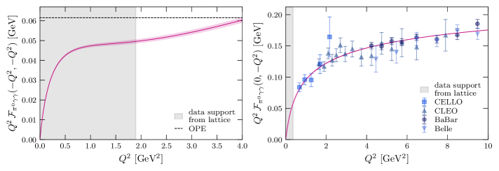
Figure 17: Transition form factor from the combined fit to lattice and experimental data for diagonal (left) and single-virtual (right) kinematics. For the diagonal kinematics, the OPE prediction for large $Q^{2}$ is indicated by the horizontal dashed line while for the single-virtual kinematics, experimental values from CELLO CELLO:1990klc , CLEO CLEO:1997fho , BaBar BaBar:2009rrj ; BaBar:2011nrp and Belle Belle:Uehara2012 are shown. The region with direct support from lattice data is shaded in grey.

Secondly, we can test the stability of the lattice-driven determination of $a_{\mu}^{\pi^{0}-\mathrm{pole}}$, $\Gamma(\pi\to\gamma\gamma)$ and $b_{\pi}$. For these quantities we obtain from the combined fit to the lattice and experimental data

$$\begin{gathered}a_{\mu}^{\pi^{0}-\mathrm{pole}}=61.7(2.0)_{\mathrm{stat}}(0.5)_{\mathrm{sys}}[2.0]_{\mathrm{tot}}\times 10^{-11},\\ \Gamma(\pi\to\gamma\gamma)=7.97(0.35)_{\mathrm{stat}}(0.11)_{\mathrm{sys}}[0.37]_{\mathrm{tot}}\,\mathrm{eV},\\ b_{\pi}=2.336(0.049)_{\mathrm{stat}}(0.018)_{\mathrm{sys}}[0.052]_{\mathrm{tot}}\,\mathrm{GeV}^{-2}.\end{gathered}$$ (56)

While these quantities are now much better determined with errors reduced by factors of 1.4, 1.6 and 3.8, the values are still fully compatible with the lattice-only determinations in Eq. (55) in Sec. VI, with the largest shift observed in $a_{\mu}^{\pi^{0}-\mathrm{pole}}$ upwards by about 1.5$\sigma$. This is easy to understand from the fact that the experimental data shifts the TFF to slightly larger values for $Q^{2}\gtrsim 2.5\text{ GeV}^{2}$ outside the lattice support, and the fact that this momentum region may still contribute up to 3% to the total value of $a_{\mu}^{\pi^{0}-\mathrm{pole}}$, cf., for example, FIG.12. Nevertheless, this exercise shows that the low-energy quantities $a_{\mu}^{\pi^{0}-\mathrm{pole}}$, $\Gamma(\pi\to\gamma\gamma)$ and $b_{\pi}$ are not very sensitive to the large-$Q^{2}$ behavior of the TFF and can safely be determined from the lattice alone.

Thirdly, for phenomenological analyses where the large-$Q^{2}$ behavior of the TFF is important, the lattice- and data-driven parameterization given here is most useful. However, we would like to add the cautionary remark that our analysis does not contain a full systematic analysis of the dependence on higher-orders in the $z$-expansion fits. We likely expect that the corresponding systematic error leads to an increased total error for the TFFs, in particular for those close to diagonal virtuality where there is no support from lattice or experimental data.

VIII Conclusions and outlook

We have presented an ab-initio computation of the pion transition form factor at the physical point in the continuum limit using twisted-mass lattice QCD, covering the kinematic range relevant for the extraction of the pion-pole contribution to the HLbL. We are able to include all disconnected Wick contractions contributing to the amplitudes and hence relevant for the calculation of the form factors.

This allows us to provide a parameterization of the transition form factor through the modified $z$-expansion including the determination of correlations between all coefficients. Our results in the double-virtual and low-$Q^{2}$, single-virtual regimes are complementary to the currently available single-virtual experimental data. Our data in the latter regime is of particular interest as new experimental data will become available Ablikim_2020 which can be compared with our prediction from first principles.

In the single-virtual regime we find agreement between our calculated pion form factor and the experimental data up to $Q_{2}^{2}\lesssim 2\text{ GeV}^{2}$, while the extrapolation to $Q_{2}^{2}\gtrsim 2\text{ GeV}^{2}$, based purely on our lattice data, systematically undershoots the experimental data from CELLO CELLO:1990klc , CLEO CLEO:1997fho , BaBar BaBar:2009rrj ; BaBar:2011nrp and Belle Belle:Uehara2012 , cf. FIG. 15. In contrast, our results for the partial decay width $\Gamma(\pi\to\gamma\gamma)$ and the slope parameter $b_{\pi}$ are compatible with the experimental values, cf. FIG. 16. We note, however, that we do not observe any significant tension between the lattice data and the experimental one, as discussed in Sec. VII.

The main result of this paper, namely the pion-pole contribution to HLbL,

$$a_{\mu}^{\pi^{0}-\mathrm{pole}}=56.7(3.1)_{\mathrm{stat}}(1.0)_{\mathrm{sys}}[3.2]_{\mathrm{tot}}\times 10^{-11},$$ (57)

is compatible with recent lattice and data-driven results, with a relative total error at thesub-6% level. The main systematic effect not fully accounted for in this work is the effect of working at a fixed finite spatial volume. On general grounds finite-size effects can be estimated in QCD to be of the order ${\cal O}(\exp(-m_{\pi}L))$, i.e., they are exponentially suppressed. With our values of $m_{\pi}L=3.6$–$3.9$ we expect them to be at most a few percent. In practice, at the physical lattice sizes of $5.1$–$5.5$ fm employed in this work, finite-size effects appear to be negligible compared to the current precision for $a_{\mu}^{\pi^{0}-\mathrm{pole}}$ and $\Gamma(\pi\to\gamma\gamma)$, as demonstrated in Ref. Gerardin:2023naa for similar physical lattice sizes. Since there are no lattice results available from previous work for the slope parameter and its sensitivity to finite-size effects, we can not exclude it to be affected more. We leave the study of finite-size effects as future work, potentially using ETMC ensembles at physical pion mass and the same range of lattice spacings with larger lattice sizes up to $\approx 7.5\,$fm.

To achieve further precision in future work, several options are available: One can use momentum $\vec{p}\neq 0$ for the pseudoscalar creation operator (i.e., the moving frame) to give a better coverage of the single-virtual axis. In addition, a fourth physical point ensemble with approximately the same volume as the three used here, but with an even smaller lattice spacing, is currently in production and could then also be included in this calculation.

Appendix A 3d Integral representation weights

The weight functions $w_{1,2}$ appearing in Eqs. (46) and (47) presented here are taken from PhysRevD.94.053006 and have been derived in Jegerlehner2009 using the method of Gegenbauer polynomials PhysRev.136.B1111 ; PhysRev.163.1699 ; ROSNER196711 ; PhysRevD.9.421 ; PhysRevD.20.2068 .

The weight functions read

$$w_{1}(Q_{1},Q_{2},\tau) =\left(-\frac{2\pi}{3}\right)\sqrt{1-\tau^{2}}\frac{Q_{1}^{3}Q_{2}^{3}}{Q_{2}^{2}+m_{\pi}^{2}}I_{1}(Q_{1},Q_{2},\tau),$$ (58)

$$w_{2}(Q_{1},Q_{2},\tau) =\left(-\frac{2\pi}{3}\right)\sqrt{1-\tau^{2}}\frac{Q_{1}^{3}Q_{2}^{3}}{(Q_{1}+Q_{2})^{2}+m_{\pi}^{2}}I_{2}(Q_{1},Q_{2},\tau),$$ (59)

with

$$I_{1}(Q_{1},Q_{2},\tau) =X(Q_{1},Q_{2},\tau)[8P_{1}P_{2}Q_{1}Q_{2}\tau-2P_{1}P_{3}(Q_{2}^{4}/m_{\mu}^{2}-2Q_{2}^{2})$$

$$\quad+4P_{2}P_{3}Q_{1}^{2}-4P_{2}-2P_{1}(2-Q_{2}^{2}/m_{\mu}^{2}+2Q_{1}Q_{2}\tau/m_{\mu}^{2})$$

$$\quad-2P_{3}(4+Q_{1}^{2}/m_{\mu}^{2}-2Q_{2}^{2}/m_{\mu}^{2})+2/m_{\mu}^{2}]$$

$$-2P_{1}P_{2}(1+(1-R_{m1})Q_{1}Q_{2}\tau/m_{\mu}^{2})$$

$$+P_{1}P_{3}(2-(1-R_{m1})Q_{2}^{2}/m_{\mu}^{2})$$

$$+P_{2}P_{3}(2+(1-R_{m1})^{2}Q_{1}Q_{2}\tau/m_{\mu}^{2})$$

$$+P_{1}(1-R_{m1})/m_{\mu}^{2}+3P_{3}(1-R_{m1})/m_{\mu}^{2}$$ (60)

and

$$I_{2}(Q_{1},Q_{2},\tau) =X(Q_{1},Q_{2},\tau)[4P_{1}P_{2}Q_{1}Q_{2}\tau+2P_{1}P_{3}Q_{2}^{2}-2P_{1}$$

$$\quad+2P_{2}P_{3}Q_{1}^{2}-2P_{2}-4P_{3}-4/m_{\mu}^{2}]$$

$$-2P_{1}P_{2}-3P_{1}(1-R_{m2})/(2m_{\mu}^{2})-3P_{2}(1-R_{m1})/(2m_{\mu}^{2})$$

$$-P_{3}(2-R_{m1}-R_{m2})/(2m_{\mu}^{2})$$

$$+P_{1}P_{3}[2+3(1-R_{m2})Q_{2}^{2}/(2m_{\mu}^{2})+(1-R_{m2})^{2}Q_{1}Q_{2}\tau/(2m_{\mu}^{2})]$$

$$+P_{2}P_{3}[2+3(1-R_{m1})Q_{1}^{2}/(2m_{\mu}^{2})+(1-R_{m1})^{2}Q_{1}Q_{2}\tau/(2m_{\mu}^{2})],$$ (61)

where

$$Q_{3}^{2} =(Q_{1}+Q_{2})^{2}=Q_{1}^{2}+2Q_{1}Q_{2}\tau+Q_{2}^{2},$$ (62)

$$\tau =\cos\theta,$$ (63)

$$P_{i} =1/Q_{i}^{2},i\in\{1,2,3\}.$$ (64)

Further,

$$X(Q_{1}Q_{2},\tau) =\frac{1}{Q_{1}Q_{2}x}\arctan\left(\frac{zx}{1-z\tau}\right),$$ (65)

$$x =\sqrt{1-\tau^{2}},$$ (66)

$$z =\frac{Q_{1}Q_{2}}{4m_{\mu}^{2}}(1-R_{m1})(1-R_{m2}),$$ (67)

$$R_{mi} =\sqrt{1+\frac{4m_{\mu}^{2}}{Q_{i}^{2}}},i\in\{1,2\}.$$ (68)

For a detailed discussion of the behavior of $w_{1,2}$ in different limits see PhysRevD.94.053006 .

Appendix B Correlation matrix for the combined fit to lattice and experimental data

Here we provide the correlation matrix for the combined fit of the modified $z$-expansion as desrcibed in Sec. VII using the coefficient set $c_{nm}=\{c_{00},c_{10},c_{11},c_{22}\}$ with the corresponding lattice-artefact corrections $\delta_{nm}=\{\delta_{00},\delta_{10}\}$ to the lattice and experimental data,

$$\mathrm{cor}(c_{nm})=\left(\begin{array}[]{cccc}+1.00&-0.14&+0.54&-0.78\\ -0.14&+1.00&-0.12&-0.06\\ +0.54&-0.12&+1.00&+0.07\\ -0.78&-0.06&+0.07&+1.00\end{array}\right)\,.$$ (69)

We refrain from providing the corresponding corner plot, since it serves the purpose of illustration only.

References

- (1) Muon g-2 collaboration, B. Abi, T. Albahri, S. Al-Kilani, D. Allspach, L. P. Alonzi, A. Anastasi et al., Measurement of the Positive Muon Anomalous Magnetic Moment to 0.46 ppm, Phys. Rev. Lett. 126 (2021) 141801, [2104.03281].
- (2) Muon g-2 collaboration, D. P. Aguillard et al., Measurement of the Positive Muon Anomalous Magnetic Moment to 0.20 ppm, 2308.06230.
- (3) G. W. Bennett and Others, Final Report of the Muon E821 Anomalous Magnetic Moment Measurement at BNL, Phys. Rev. D 73 (2006) 72003, [0602035].
- (4) T. Aoyama, N. Asmussen, M. Benayoun, J. Bijnens, T. Blum, M. Bruno et al., The anomalous magnetic moment of the muon in the Standard Model, Phys. Rept. 887 (2020) 1–166, [2006.04822].
- (5) T. Blum, S. Chowdhury, M. Hayakawa and T. Izubuchi, Hadronic light-by-light scattering contribution to the muon anomalous magnetic moment from lattice QCD, Phys. Rev. Lett. 114 (2015) 012001, [1407.2923].
- (6) T. Blum, N. Christ, M. Hayakawa, T. Izubuchi, L. Jin and C. Lehner, Lattice Calculation of Hadronic Light-by-Light Contribution to the Muon Anomalous Magnetic Moment, Phys. Rev. D 93 (2016) 014503, [1510.07100].
- (7) T. Blum, N. Christ, M. Hayakawa, T. Izubuchi, L. Jin, C. Jung et al., Connected and Leading Disconnected Hadronic Light-by-Light Contribution to the Muon Anomalous Magnetic Moment with a Physical Pion Mass, Phys. Rev. Lett. 118 (2017) 022005, [1610.04603].
- (8) T. Blum, N. Christ, M. Hayakawa, T. Izubuchi, L. Jin, C. Jung et al., Using infinite volume, continuum QED and lattice QCD for the hadronic light-by-light contribution to the muon anomalous magnetic moment, Phys. Rev. D 96 (2017) 034515, [1705.01067].
- (9) E. H. Chao, R. J. Hudspith, A. Gérardin, J. R. Green, H. B. Meyer and K. Ottnad, Hadronic light-by-light contribution to from lattice QCD: a complete calculation, Eur. Phys. J. C 81 (2021) 5–11, [2104.02632].
- (10) E.-H. Chao, R. J. Hudspith, A. Gérardin, J. R. Green and H. B. Meyer, The charm-quark contribution to light-by-light scattering in the muon from lattice QCD, Eur. Phys. J. C 82 (2022) 664, [2204.08844].
- (11) N. Asmussen, E.-H. Chao, A. Gérardin, J. R. Green, R. J. Hudspith, H. B. Meyer et al., Hadronic light-by-light scattering contribution to the muon from lattice QCD: semi-analytical calculation of the QED kernel, JHEP 04 (2023) 040, [2210.12263].
- (12) G. Colangelo, M. Hoferichter, M. Procura and P. Stoffer, Dispersive approach to hadronic light-by-light scattering, JHEP 2014 (2014) 1–33, [1402.7081].
- (13) G. Colangelo, M. Hoferichter, B. Kubis, M. Procura and P. Stoffer, Towards a data-driven analysis of hadronic light-by-light scattering, Phys. Lett. B 738 (2014) 6–12, [1408.2517].
- (14) G. Colangelo, M. Hoferichter, M. Procura and P. Stoffer, Dispersion relation for hadronic light-by-light scattering: theoretical foundations, JHEP 09 (2015) 074, [1506.01386].
- (15) V. Pauk and M. Vanderhaeghen, Anomalous magnetic moment of the muon in a dispersive approach, Phys. Rev. D 90 (2014) 113012, [1409.0819].
- (16) M. Knecht and A. Nyffeler, Hadronic light by light corrections to the muon : The Pion pole contribution, Phys. Rev. D 65 (2002) 73034, [0111058].
- (17) A. Nyffeler, Precision of a data-driven estimate of hadronic light-by-light scattering in the muon : Pseudoscalar-pole contribution, Phys. Rev. D 94 (2016) 53006.
- (18) F. Jegerlehner and A. Nyffeler, The muon , Phys. Rept. 477 (2009) 1–110, [0902.3360].
- (19) CELLO collaboration, H. J. Behrend et al., A Measurement of the , and -prime electromagnetic form-factors, Z. Phys. C 49 (1991) 401–410.
- (20) CLEO collaboration, J. Gronberg et al., Measurements of the meson - photon transition form-factors of light pseudoscalar mesons at large momentum transfer, Phys. Rev. D 57 (1998) 33–54, [hep-ex/9707031].
- (21) BaBar collaboration, B. Aubert et al., Measurement of the transition form factor, Phys. Rev. D 80 (2009) 052002, [0905.4778].
- (22) BaBar collaboration, P. del Amo Sanchez et al., Measurement of the and transition form factors, Phys. Rev. D 84 (2011) 052001, [1101.1142].
- (23) Belle Collaboration collaboration, S. Uehara, Y. Watanabe, H. Nakazawa, I. Adachi, H. Aihara, D. M. Asner et al., Measurement of transition form factor at belle, Phys. Rev. D 86 (2012-11) 092007.
- (24) P. Masjuan and P. Sanchez-Puertas, Pseudoscalar-pole contribution to the : A rational approach, Phys. Rev. D 95 (2017) 1–19, [1701.05829].
- (25) M. Hoferichter, B.-L. Hoid, B. Kubis, S. Leupold and S. P. Schneider, Pion-pole contribution to hadronic light-by-light scattering in the anomalous magnetic moment of the muon, Phys. Rev. Lett. 121 (2018) 112002, [1805.01471].
- (26) M. Hoferichter, B.-L. L. Hoid, B. Kubis, S. Leupold and S. P. Schneider, Dispersion relation for hadronic light-by-light scattering: pion pole, JHEP 10 (2018) 141, [1808.04823].
- (27) A. Gérardin, H. B. Meyer and A. Nyffeler, Lattice calculation of the pion transition form factor , Phys. Rev. D 94 (2016) 74507, [1607.08174].
- (28) A. Gérardin, H. B. Meyer and A. Nyffeler, Lattice calculation of the pion transition form factor with Wilson quarks, Phys. Rev. D 100 (2019) 34520, [1903.09471].
- (29) A. Gérardin, W. E. A. Verplanke, G. Wang, Z. Fodor, J. N. Guenther, L. Lellouch et al., Lattice calculation of the , and transition form factors and the hadronic light-by-light contribution to the muon , 2305.04570.
- (30) S. Burri, C. Alexandrou, S. Bacchio, G. Bergner, J. Finkenrath, A. Gasbarro et al., Pion-pole contribution to HLbL from twisted mass lattice QCD at the physical point, PoS LATTICE2021 (2022) 519, [2112.03586].
- (31) S. Burri, G. Kanwar, C. Alexandrou, S. Bacchio, G. Bergner, J. Finkenrath et al., Pseudoscalar-pole contributions to the muon at the physical point, PoS LATTICE2022 (2023) 306, [2212.10300].
- (32) C. Alexandrou, S. Bacchio, S. Burri, J. Finkenrath, A. Gasbarro, K. Hadjiyiannakou et al., The transition form factor and the hadronic light-by-light -pole contribution to the muon from lattice QCD, 2212.06704.
- (33) X.-d. X. Ji and C.-w. C. Jung, Studying hadronic structure of the photon in lattice QCD, Phys. Rev. Lett. 86 (2001) 208, [0101014].
- (34) X.-d. Ji and C.-w. Jung, Photon structure functions from quenched lattice QCD, Phys. Rev. D 64 (2001) 34506, [0103007].
- (35) J. J. Dudek and R. G. Edwards, Two Photon Decays of Charmonia from Lattice QCD, Phys. Rev. Lett. 97 (2006) 172001, [0607140].
- (36) R. Frezzotti and G. C. Rossi, Chirally improving Wilson fermions. 1. O(a) improvement, JHEP 08 (2004) 007, [hep-lat/0306014].
- (37) Alpha collaboration, R. Frezzotti, P. A. Grassi, S. Sint and P. Weisz, Lattice QCD with a chirally twisted mass term, JHEP 08 (2001) 058, [hep-lat/0101001].
- (38) R. Frezzotti and G. C. Rossi, Chirally improving Wilson fermions. II. Four-quark operators, JHEP 10 (2004) 070, [hep-lat/0407002].
- (39) C. Alexandrou et al., Simulating twisted mass fermions at physical light, strange and charm quark masses, Phys. Rev. D 98 (2018) 054518, [1807.00495].
- (40) G. Bergner, P. Dimopoulos, J. Finkenrath, E. Fiorenza, R. Frezzotti, M. Garofalo et al., Quark masses and decay constants in isoQCD with Wilson clover twisted mass fermions, PoS LATTICE2019 (2020) 181, [2001.09116].
- (41) Extended Twisted Mass collaboration, C. Alexandrou, S. Bacchio, G. Bergner, P. Dimopoulos, J. Finkenrath, R. Frezzotti et al., Ratio of kaon and pion leptonic decay constants with Wilson-clover twisted-mass fermions, Phys. Rev. D 104 (2021) 74520, [2104.06747].
- (42) J. Finkenrath, C. Alexandrou, S. Bacchio, M. Constantinou, P. Dimopoulos, R. Frezzotti et al., Twisted mass gauge ensembles at physical values of the light, strange and charm quark masses, PoS LATTICE2021 (2022) 284, [2201.02551].
- (43) Extended Twisted Mass collaboration, C. Alexandrou et al., Lattice calculation of the short and intermediate time-distance hadronic vacuum polarization contributions to the muon magnetic moment using twisted-mass fermions, Phys. Rev. D 107 (2023) 074506, [2206.15084].
- (44) A. Stathopoulos, J. Laeuchli and K. Orginos, Hierarchical probing for estimating the trace of the matrix inverse on toroidal lattices, 1302.4018.
- (45) A. S. Gambhir, A. Stathopoulos and K. Orginos, Deflation as a Method of Variance Reduction for Estimating the Trace of a Matrix Inverse, SIAM J. Sci. Comput. 39 (2017) A532–A558, [1603.05988].
- (46) C. Alexandrou, S. Bacchio, M. Constantinou, J. Finkenrath, K. Hadjiyiannakou, K. Jansen et al., Complete flavor decomposition of the spin and momentum fraction of the proton using lattice QCD simulations at physical pion mass, Phys. Rev. D 101 (2020) 094513, [2003.08486].
- (47) C. Alexandrou et al., Disconnected contribution to the LO HVP term of muon g-2 from ETMC, PoS LATTICE2022 (2023) 303, [2212.07057].
- (48) B. Moussallam, Chiral sum rules for parameters and its application to ,,’ decays, Phys. Rev. D 51 (1995) 4939–4949.
- (49) M. Knecht, S. Peris, M. Perrottet and E. de Rafael, Decay of Pseudoscalars into Lepton Pairs and Large- QCD, Phys. Rev. Lett. 83 (1999) 5230–5233.
- (50) S. L. Adler, Axial-Vector Vertex in Spinor Electrodynamics, Phys. Rev. 177 (1969) 2426–2438.
- (51) J. S. Bell and R. Jackiw, A PCAC puzzle: in the -model, Nuovo Cimento A 60 (1969) 47–61.
- (52) Particle Data Group collaboration, R. L. Workman and Others, Review of Particle Physics, PTEP 2022 (2022) 083C01.
- (53) G. P. Lepage and S. J. Brodsky, Exclusive Processes in Quantum Chromodynamics: Evolution Equations for Hadronic Wave Functions and the Form-Factors of Mesons, Phys. Lett. B 87 (1979) 359–365.
- (54) G. P. Lepage and S. J. Brodsky, Exclusive Processes in Perturbative Quantum Chromodynamics, Phys. Rev. D 22 (1980) 2157.
- (55) S. J. Brodsky and G. P. Lepage, Large Angle Two Photon Exclusive Channels in Quantum Chromodynamics, Phys. Rev. D 24 (1981) 1808.
- (56) V. A. Nesterenko and A. V. Radyushkin, Comparison of the QCD Sum Rule Approach and Perturbative QCD Analysis for Process, Sov. J. Nucl. Phys. 38 (1983) 284.
- (57) V. A. Novikov, M. A. Shifman, A. I. Vainshtein, M. B. Voloshin and V. I. Zakharov, Use and Misuse of QCD Sum Rules, Factorization and Related Topics, Nucl. Phys. B 237 (1984) 525–552.
- (58) C. G. Boyd, B. Grinstein and R. F. Lebed, Model independent determinations of , form-factors, Nucl. Phys. B 461 (1996) 493–511, [9508211].
- (59) C. Bourrely, I. Caprini and L. Lellouch, Model-independent description of decays and a determination of , Phys. Rev. D 79 (2009) 013008, [0807.2722].
- (60) PrimEx collaboration, I. Larin et al., A New Measurement of the Radiative Decay Width, Phys. Rev. Lett. 106 (2011) 162303, [1009.1681].
- (61) I. Larin, Y. Zhang, A. Gasparian, L. Gan, R. Miskimen, M. Khandaker et al., Precision measurement of the neutral pion lifetime, Science 368 (2020) 506–509, [https://www.science.org/doi/pdf/10.1126/science.aay6641].
- (62) H. Akaike, A Bayesian analysis of the minimum AIC procedure, Annals of the Institute of Statistical Mathematics 30 (1978) 9–14.
- (63) W. I. Jay and E. T. Neil, Bayesian model averaging for analysis of lattice field theory results, Phys. Rev. D 103 (2021) , [2008.01069].
- (64) S. Borsanyi, S. Durr, Z. Fodor, C. Hoelbling, S. D. Katz, S. Krieg et al., Ab initio calculation of the neutron-proton mass difference, Science 347 (2015) 1452–1455.
- (65) S. Borsanyi, Z. Fodor, J. N. Guenther, C. Hoelbling, S. D. Katz, L. Lellouch et al., Leading hadronic contribution to the muon magnetic moment from lattice QCD, Nature 593 (2021) 51–55, [2002.12347].
- (66) Extended Twisted Mass collaboration, C. Alexandrou, S. Bacchio, G. Bergner, M. Constantinou, M. D. Carlo, P. Dimopoulos et al., Quark masses using twisted-mass fermion gauge ensembles, Phys. Rev. D 104 (2021) 074515, [2104.13408].
- (67) P. Masjuan, transition form factor at low-energies from a model-independent approach, Phys. Rev. D 86 (2012) 094021, [1206.2549].
- (68) M. Ablikim, M. N. Achasov, P. Adlarson, S. Ahmed, M. Albrecht, M. Alekseev et al., Future physics programme of BESIII, Chinese Physics C 44 (2020) 040001.
- (69) D. Krause, JUWELS: Modular Tier-0/1 Supercomputer at the Jülich Supercomputing Centre, JLSRF 5 (2019) A135.
- (70) K. Jansen and C. Urbach, tmLQCD: A Program suite to simulate Wilson Twisted mass Lattice QCD, Comput. Phys. Commun. 180 (2009) 2717–2738, [0905.3331].
- (71) A. Deuzeman, K. Jansen, B. Kostrzewa and C. Urbach, Experiences with OpenMP in tmLQCD, PoS LATTICE2013 (2014) 416, [1311.4521].
- (72) A. Abdel-Rehim, F. Burger, A. Deuzeman, K. Jansen, B. Kostrzewa, L. Scorzato et al., Recent developments in the tmLQCD software suite, PoS LATTICE2013 (2014) 414, [1311.5495].
- (73) B. Kostrzewa, S. Bacchio, J. Finkenrath, M. Garofalo, F. Pittler, S. Romiti et al., Twisted mass ensemble generation on GPU machines, 2022-12. 2212.06635.
- (74) C. Alexandrou, S. Bacchio, J. Finkenrath, A. Frommer, K. Kahl and M. Rottmann, Adaptive Aggregation-based Domain Decomposition Multigrid for Twisted Mass Fermions, Phys. Rev. D 94 (2016) 114509, [1610.02370].
- (75) C. Alexandrou, S. Bacchio and J. Finkenrath, Multigrid approach in shifted linear systems for the non-degenerated twisted mass operator, Comput. Phys. Commun. 236 (2019) 51–64, [1805.09584].
- (76) M. A. Clark, R. Babich, K. Barros, R. C. Brower and C. Rebbi, Solving Lattice QCD systems of equations using mixed precision solvers on GPUs, Comput. Phys. Commun. 181 (2010) 1517–1528, [0911.3191].
- (77) R. Babich, M. A. Clark, B. Joo, G. Shi, R. C. Brower and S. Gottlieb, Scaling Lattice QCD beyond 100 GPUs, in SC11 International Conference for High Performance Computing, Networking, Storage and Analysis, 2011-09. 1109.2935. DOI.
- (78) M. A. Clark, B. Joó, A. Strelchenko, M. Cheng, A. Gambhir and R. Brower, Accelerating Lattice QCD Multigrid on GPUs Using Fine-Grained Parallelization, 1612.07873.
- (79) J. D. Hunter, Matplotlib: A 2d graphics environment, Computing in Science & Engineering 9 (2007) 90–95.
- (80) D. Foreman-Mackey, corner.py: Scatterplot matrices in python, The Journal of Open Source Software 1 (jun, 2016) 24.
- (81) K. Johnson, M. Baker and R. Willey, Self-Energy of the Electron, Phys. Rev. 136 (1964) B1111—-B1119.
- (82) K. Johnson, R. Willey and M. Baker, Vacuum Polarization in Quantum Electrodynamics, Phys. Rev. 163 (1967) 1699–1715.
- (83) J. L. Rosner, Higher-order contributions to the divergent part of in a model quantum electrodynamics, Annals of Physics 44 (1967) 11–34.
- (84) M. J. Levine and R. Roskies, Hyperspherical approach to quantum electrodynamics: sixth-order magnetic moment, Phys. Rev. D 9 (1974) 421–429.
- (85) M. J. Levine, E. Remiddi and R. Roskies, Analytic contributions to the factor of the electron in sixth order, Phys. Rev. D 20 (1979) 2068–2076.