Improving Generative Model-based Unfolding with Schrödinger Bridges

Abstract

Machine learning-based unfolding has enabled unbinned and high-dimensional differential cross section measurements. Two main approaches have emerged in this research area: one based on discriminative models and one based on generative models. The main advantage of discriminative models is that they learn a small correction to a starting simulation while generative models scale better to regions of phase space with little data. We propose to use Schrödinger Bridges and diffusion models to create SBUnfold, an unfolding approach that combines the strengths of both discriminative and generative models. The key feature of SBUnfold is that its generative model maps one set of events into another without having to go through a known probability density as is the case for normalizing flows and standard diffusion models. We show that SBUnfold achieves excellent performance compared to state of the art methods on a synthetic $Z$+jets dataset.

I Introduction

Correcting detector effects – called deconvolution or unfolding – is the central statistical task in differential cross section measurements in particle, nuclear, and astrophysics. Classical unfolding methods are based on histograms, which result in binned measurements in a small number of dimensions. Machine learning has the potential to revolutionize differential cross section measurements by enabling unbinned and high-dimensional measurements. A number of machine learning-based unfolding techniques have been proposed [1, 2, 3, 4, 5, 6, 7, 8, 9, 10, 11, 12, 13, 14, 15] (see also Ref. [16] for an overview) and the OmniFold method [5, 9] has recently been applied to studies of hadronic final states with data from H1 [17, 18, 19, 20], LHCb [21], CMS [22], and STAR [23].

Let $X$ represent an event at detector-level and $Z$ represent the same event at particle-level. The goal of unfolding is to infer the most likely density $p(z)$ using simulated pairs $(Z,X)$ and observations $x$ from data. In classical approaches, $X$ and $Z$ are discretized and unfolding proceeds via regularized matrix inversion to approximate the maximum likelihood solution. The likelihood is a product of Poisson probability mass functions, although most measurements do not directly maximize this likelihood. For example, one of the most common classical unfolding algorithms is called Lucy-Richardson deconvolution [24, 25] (also known as Iterative Bayesian Unfolding [26]) which uses an Expectation-Maximization (EM) algorithm to converge to a maximum likelihood estimator.

In the unbinned case, the likelihood is not known. One solution is to use the EM algorithm, which is at the core of two maximum likelihood machine learning approaches. The first is OmniFold, which proceeds as follows:

E step

$\omega_{i+1}(x)=p_{\text{data}}(x)/\tilde{p}_{\text{sim.}}(x)$

$\tilde{p}_{\text{sim.}}(x)\equiv\int\text{d}z\,p_{\text{sim.}}(x,z)\,\nu_{i}(z)$

M step

$\nu_{i+1}(z)=\bar{p}_{\text{sim.}}(z)/p_{\text{sim.}}(z)$

$\bar{p}_{\text{sim.}}(z)\equiv\int\text{d}x\,p_{\text{sim.}}(x,z)\,\omega_{i+1}(x)$

Both the Expectation (E) and Maximization (M) steps are achieved in practice by training classifiers and interpreting the resulting score as the target likelihood ratio, e.g. take samples from $p_{\text{data}}$ and from $\tilde{p}_{\text{sim.}}$ (samples from $p_{\text{sim.}}$ weighted by $\nu$) and train a classifier to distinguish them for the E step. The final result is the set of simulated events weighted by $\nu$ with probability density $p_{\text{sim.}}(z)\,\nu(z)$ in the continuum limit. An alternative approach called IcINN [11] is instead based on generative models:

E step

$p_{i}(z|x)\propto p_{\text{sim.}}(x|z)\,\nu_{i}(z)$

M step

$\nu_{i+1}(z)=\check{p}_{\text{sim.}}(z)/p_{\text{sim.}}(z)$

$\check{p}_{\text{sim.}}(z)\equiv\int\text{d}x\,p_{i}(z|x)\,p_{\text{data}}(x)$

The E step of the IcINN is achieved by training a generative model (a normalizing flow [27]) to emulate $p_{\text{sim.}}(x|z)\,\nu_{i}(z)$ while the M step uses a classifier as in OmniFold. The groundwork for the IcINN was laid in Ref. [7], which focused on the E step, as have other papers using normalizing flows, diffusion models, and generative adversarial networks [2, 6, 14]. Comparing both the E and M steps of OmniFold and the IcINN, one can see that they are formally the same and thus the EM proof in Ref. [5] applies to both approaches.

While formally both algorithms achieve the same EM algorithm step by step, they have complementary strengths in practice. One of OmniFold’s strengths is that it starts from an existing simulation and if that simulation is close to nature, then the neural networks only have to learn a small correction. In contrast, the normalizing flows in IcINN have to map a known probability density (e.g. a multidimensional Gaussian) to the data and these can be quite different. However, the E step of OmniFold trains directly on data and thus its performance degrades when there are not many events. In contrast, the E step of the IcINN is trained using simulation and so can better handle the case of fewer events.

We propose an approach called SBUnfold that incorporates strengths of both OmniFold and the IcINN. We employ a technique called a Schrödinger Bridge (SB) using a diffusion model to learn the generative model in the IcINN workflow. In contrast to a normalizing flow or standard diffusion model, a Schrödinger Bridge learns to map one dataset into another without needing to know the probability density of one of the datasets. Thus, the Schrödinger Bridge should ideally learn a small correction while also preserving the E step learning with simulation and not data. The latter property means that SBUnfold should outperform OmniFold when there are few events in data. Since OmniFold and the IcINN differ only in the E step, we focus exclusively on the E step of the first iteration for all methods and will refer to IcINN as cINN for disambiguation.

This paper is organized as follows. Section II introduces Schrödinger Bridges and Sec. III describes how this can be used for unfolding. Numerical results from the OmniFold public $Z$+jets dataset are presented in Sec. IV. The paper ends with conclusions and outlook in Sec. V.

II Schrodinger Bridge and the connection with Diffusion Models

Diffusion models have become popular choices for generative modeling due to their large degree of flexibility, stable training, and often competitive results compared to other approaches. The core idea is to design a time-dependent perturbation process that slowly perturbs data towards a tractable noise distribution. The goal of the generative model is to then reverse this process, starting from a noise sample and denoising towards new data observations. From a fixed choice of stochastic differential equation (SDE)

$$\mathrm{d}\textbf{x}=f(\textbf{x},t)\mathrm{d}t+g(t)\mathrm{dw},$$ (1)

described by parameters $f(\textbf{x},t)\in\mathbb{R}^{d}$ and $g(t)\in\mathbb{R}$, the evolution over time of the data observation $\textbf{x}\in\mathbb{R}^{d}$ is determined. The same initial data point can undergo different paths due to the additional stochastic term identified by the Wiener process, or Brownian motion, w$(t)\in\mathbb{R}^{d}$, often sampled from a normal distribution with the same dimension as the data. The reverse process follows the reverse SDE equation that reads:

$$\mathrm{d}\textbf{x}=[f(\textbf{x},t)-g(t)^{2}\nabla\log p(\textbf{x},t)]\mathrm{d}t+g(t)\mathrm{d\bar{w}}.$$ (2)

The only unknown term in the Eq. 2 is the score function, $\nabla\log p(\textbf{x},t)$, which can be approximated using denoising score matching [29] and minimizing the loss function

$$\mathcal{L}_{SGM}=\frac{1}{2}\mathbb{E}_{\textbf{x}_{t},t}\left\|\epsilon_{\theta}(\textbf{x}_{t},t)-\sigma_{t}\nabla_{\textbf{x}_{t}}\log q(\textbf{x}_{t}|\textbf{x})\right\|^{2}_{2},$$ (3)

where a neural network with trainable parameters $\theta$ is optimized to approximate the score function of data that have been perturbed by a Gaussian distribution with time-dependent parameters $\alpha_{t}$ and $\sigma_{t}$. For this Gaussian perturbation, $q(\textbf{x}_{t}|\textbf{x})=\mathcal{N}(\textbf{x}_{t},\alpha_{t}\textbf{x},\sigma_{t}^{2}\textbf{I})$, requiring $f(\textbf{x},t)$ to be affine with respect x and resulting in a Gaussian noise at the end of the diffusion process. For an arbitrary noise distribution, the corresponding choice of $f(\textbf{x},t)$ cannot be easily identified, often restricting the family of distributions one is allowed to choose for the diffusion process. A more general framework that allows the mapping between general distributions corresponds to the solution of the Schrödinger Bridge (SB) problem. Initially proposed by Erwin Schrödinger [30], the problem concerned the inference of the trajectories from particles undergoing a diffusion process where experimental observations of the particle’s trajectory are available only at specific time values, fixing the boundary conditions of the problem. The connection with diffusion generative models becomes more clear by considering the following forward and backward SDEs:

$$\mathrm{d}\textbf{x} =[f(\textbf{x},t)+g(t)^{2}\nabla\log{\Psi}(\textbf{x},t)]\mathrm{d}t+g(t)\mathrm{dw},$$ (4a)

$$\mathrm{d}\textbf{x} =[f(\textbf{x},t)-g(t)^{2}\nabla\log\hat{\Psi}(\textbf{x},t)]\mathrm{d}t+g(t)\mathrm{d\bar{w}}.$$ (4b)

The wave-functions $\Psi$ and $\hat{\Psi}$ satisfy

$$\frac{\partial{\Psi(\textbf{x},t)}}{\partial t} =-\nabla\Psi(\textbf{x},t)^{\intercal}f(\textbf{x},t)-\frac{1}{2}g(t)^{2}\Delta\Psi(\textbf{x},t)$$

$$\frac{\partial{\hat{\Psi}(\textbf{x},t)}}{\partial t} =-\nabla\cdot(\hat{\Psi}(\textbf{x},t)f(\textbf{x},t))+\frac{1}{2}g(t)^{2}\Delta\hat{\Psi}(\textbf{x},t)$$

with $\Psi(\textbf{x},0)\hat{\Psi}(\textbf{x},0)=p_{A}(\textbf{x})$ and $\Psi(\textbf{x},1)\hat{\Psi}(\textbf{x},1)=p_{B}(\textbf{x})$ for densities $p_{A}(\textbf{x})$ and $p_{B}(\textbf{x})$. Compared to Eq. 2, the presence of an additional non-linear term to the drift function, $g(t)^{2}\nabla\log\hat{\Psi}(\textbf{x},t)$, enables the diffusion between densities that are not necessarily represented by a standard normal distributions at the end of the diffusion process. Additionally, $\nabla\log\hat{\Psi}(\textbf{x},t)$ no longer represents the score function of the perturbed data, but is related to it since

$$\Psi(\textbf{x},t)\hat{\Psi}(\textbf{x},t)=q(\textbf{x},t),$$ (5)

hence

$$\nabla\log\Psi(\textbf{x},t)+\nabla\log\hat{\Psi}(\textbf{x},t)=\nabla\log q(\textbf{x},t).$$ (6)

While the equations describing the general SB problem have similarities with the standard framework for diffusion generative models, a general strategy to solve the problem is not immediately obvious. The authors of Ref. [31] propose a tractable solution named I²SB, by considering the presence of pairs of observations in the dataset such that $p(\textbf{x}_{a},\textbf{x}_{b})=p_{A}(\textbf{x}_{a})p_{B}(\textbf{x}_{b}|\textbf{x}_{a})$. This assumption also holds for the unfolding methodology where pairs of particle collisions before and after detector interactions are always available in the simulation. With this approximation, the authors of Ref. [31] have shown that by setting the linear drift term $f(\textbf{x},t){:=}0$, the posterior of Eq. 4, $q(\textbf{x}|\textbf{x}_{a},\textbf{x}_{b})$, has the analytic form:

$$q(\textbf{x}|\textbf{x}_{a},\textbf{x}_{b})=\mathcal{N}(\textbf{x}_{t};\mu_{t}(\textbf{x}_{a},\textbf{x}_{b}),\Sigma_{t}),$$ (7)

$$\mu_{t} =\frac{\bar{\sigma}_{t}^{2}}{\bar{\sigma}_{t}^{2}+\sigma^{2}_{t}}\textbf{x}_{a}+\frac{\sigma^{2}_{t}}{\bar{\sigma}_{t}^{2}+\sigma^{2}_{t}}\textbf{x}_{b},\quad\Sigma_{t}=\frac{\sigma_{t}^{2}\bar{\sigma}_{t}^{2}}{\bar{\sigma}_{t}^{2}+\sigma^{2}_{t}}\cdot I,$$ (8)

with $\sigma^{2}_{t}{:=}\int_{0}^{t}g^{2}(\tau)\mathrm{d}\tau$ and $\bar{\sigma}^{2}_{t}{:=}\int_{t}^{1}g^{2}(\tau)\mathrm{d}\tau$. From this expression, given pairs $(\textbf{x}_{a},\textbf{x}_{b})$, we can directly determine $\textbf{x}_{t}=\mu_{t}+\Sigma_{t}\epsilon$, $\epsilon\sim\mathcal{N}(0,1)^{d}$ for any time step $t$. The loss function is then identified similar to Eq. 3 as:

$$\mathcal{L}_{\mathrm{I^{2}SB}}=\frac{1}{2}\mathbb{E}_{\textbf{x}_{t},t}\left\|\epsilon_{\theta}(\textbf{x}_{t},t)-\frac{\textbf{x}_{t}-\textbf{x}_{0}}{\sigma_{t}}\right\|^{2}_{2},$$ (9)

where the right term of the loss function approximates the score function of the backward drift $\nabla\log\hat{\Psi}(\textbf{x},t)$, which can then be used during sampling to transport samples from $p_{B}$ to $p_{A}$.

During sampling, standard recursive samplers like DDPM [32] can be used with the prediction of the denoised data $\textbf{x}_{0}^{\theta}=\textbf{x}_{n+1}-\sigma_{n+1}\epsilon_{\theta}(\textbf{x}_{n+1},n+1)$ at time step $n<N$ defined as:

$$\textbf{x}_{n}\sim q(\textbf{x}_{n}|\textbf{x}_{0}^{\theta},\textbf{x}_{n+1}),\textbf{x}_{N}\sim p_{B}.$$ (10)

The stochastic solver is able to produce different observations given the same exact inputs, which can then be used for different coverage tests regarding the validity of the generated outputs. A second option is to consider the deterministic case where the posterior distributions are effectively replaced by their means. This particular case is described by the solution of the following ODE:

$$\mathrm{d}\textbf{x}_{t}=\mathbf{v}_{t}(\textbf{x}_{t}|\textbf{x}_{0})\mathrm{d}t=\frac{\beta_{t}}{\sigma_{t}^{2}}(\textbf{x}_{t}-\textbf{x}_{0})\mathrm{d}t\,,$$ (11)

which describes an optimal transport plan [33]. In our studies, we observe similar sample quality between the stochastic and deterministic settings and report the results based on the deterministic case for simplicity.

We set $f(\textbf{x},t){:=}0$ and $g(t)=\sqrt{\beta(t)}$, with $\beta(t)$ the triangular function:

$$\beta(t)=\begin{cases}\beta_{0}+2(\beta_{1}-\beta_{0})t,&0\leq t<\frac{1}{2},\\ \beta_{1}-2(\beta_{1}-\beta_{0})(t-\frac{1}{2}),&\frac{1}{2}\leq t\leq 1.\end{cases}$$ (12)

with $\beta_{0}=10^{-5}$ and $\beta_{1}=10^{-4}$.

III Unfolding Methodology

We test SBUnfold using the public dataset from Ref. [5], available on Zenodo [34] and briefly summarized in the following. Proton-proton collisions producing a $Z$ boson are generated at a center-of-mass energy of $\sqrt{s}=14$ TeV. A non-trivial test of unfolding requires at least two datasets, one that acts as the ‘data’ and one that is the ‘simulation’. For the ‘data’, collisions are simulated with the default tune of Herwig 7.1.5 [35, 36, 37]. We only make use of the reconstructed events from Herwig as would be the case with real data. The Herwig particle-level events are only used when evaluating the performance of different methods. For the ‘simulation’, events are simulated with Tune 26 [38] of Pythia 8.243 [39, 40, 41]. Detector distortions are simulated with Delphes 3.4.2 [42] and the CMS tune that uses a particle flow reconstruction. In future work, we will investigate the performance of SBUnfold on the full phase space of particles (particle-level) and particle flow objects (detector-level). For this study, we focus on a fixed set of six observables that serve as the benchmark for fixed-dimension unfolding. These observables are computed from the substructure of the leading jet. The jets are clustered using all particle flow objects at detector level and all stable non-neutrino truth particles at particle level. They are defined by the anti-$k_{T}$ algorithm [43] with radius parameter $R=0.4$ as implemented in FastJet 3.3.2 [44, 45]. The first four observables are the jet mass $m$, constituent multiplicity $M$, the $N$-subjettiness ratio $\tau_{21}=\tau_{2}^{(\beta=1)}/\tau_{1}^{(\beta=1)}$ [46, 47], and the jet width $w$ (implemented as $\tau_{1}^{(\beta=1)}$). The remaining two observables are the jet mass $\ln\rho=\ln m_{\text{SD}}^{2}/p_{T}^{2}$ and momentum fraction $z_{g}$ after Soft Drop grooming [48, 49] with $z_{\text{cut}}=0.1$ and $\beta=0$. Many of the observables are computed with FastJet Contrib 1.042 [50].

The $Z$ bosons are required to have $p_{T}>200$ GeV in order to render acceptance effects negligible. Each dataset consists of about 1.6 millon events.

The noise prediction model of SBUnfold is implemented using a fully-connected architecture incorporating multiple skip connections. Specifically, the model employs four ResNet [51] blocks, where each residual layer is connected to the output of a single-layer network through a skip connection. The activation function used is LeakyRelu [52] with a slope of $\alpha=0.01$, and all layer sizes are set to 32. The implementation of the model is carried out using Pytorch [53]. The generation is carried out by starding from data observations at reconstruction level and using the SB to move towards the generator level events using 1000 time steps to improve accuracy. The cINN implementation uses the normalizing flow model presented in Ref. [7] while the first step of the first iteration of OmniFold uses a fully-connected model with three hidden layers, ReLu activation function, and node sizes set to 50, 150, 50, before the output layer with a single node and sigmoid activation function. Both cINN and OmniFold are implemented in TensorFlow [54]. For all models, the number of trainable parameters are kept similar at around 13k. The initial learning rate is set to $10^{-3}$ and all models are trained for 30 epochs with batch size of 128. A total of 1M training events are used to train all models taken from the Pythia simulations. The pseudo-data used to evaluate the performance of the unfolding is taken from Herwig. Both SBUnfold and cINN do not have access to the data during training while OmniFold uses a total of 2M training events (1M from Pythia and 1M from Herwig). We investigate the impact of the pseudo-data training size in Sec. IV when determining the unfolded results. All trainings are carried out using the Perlmutter supercomputer with a single NVIDIA A100 GPU.

Figure 1: Comparison between different unfolding algorithms for six different physics observables unfolded. All observables are unfolded simultaneously without binning, with histograms shown only for evaluation. Results are evaluated over 600’000 pseudo-data points. Statistical uncertainties are shown only in the ratio panel. Pseudo-data and simulation are described by Pythia.

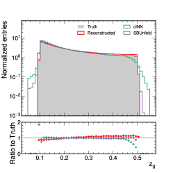
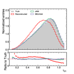
IV Results

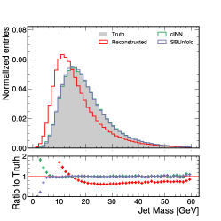
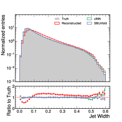
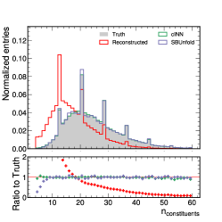
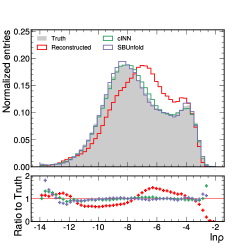
We evaluate the performance of SBUnfold compared to other unfolding methodologies by first looking at unfolded distributions where both pseudo-data and samples used to train the different unfolding methods originate from the Pythia simulation. The results showing the unfolded distributions are shown in Fig. 1. In App. A, we also provide the comparison of the results obtained by a standard diffusion model.

Figure 2: Pairwise correlation plot between all unfolded variables using the cINN (left) or SBUnfold (right) algorithms.

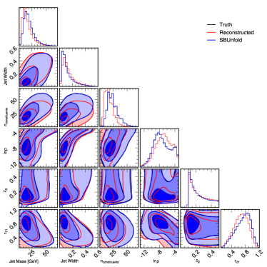
We observe a good agreement with the expected distributions from Pythia at generator level and the responses of the generative models for unfolding. We omit the OmniFold results since the weighting function becomes trivial when both data and simulation are statistically identical. We also investigate the distribution of the pairwise correlation between each pair of unfolded features to verify that SBUnfold is also capable of learning the correct correlations between distributions. The results are shown in Fig. 2.

Table 1: Comparison of the earth mover’s distance (EMD) and triangular discriminator between different algorithms. EMD is calculated over unbinned distributions while triangular discriminator uses histograms as inputs. Uncertainties from EMD are derived using 100 bootstraps with replacement taken from the unfolded data. Results are evaluated using 600’000 pseudo-data points sampled from Pythia. Quantities in bold represent the method with best performance.

Model	EMD($\times 10$)/Triangular Discriminator($\times 10^{3}$)
	cINN	SBUnfold
Jet mass	1.4$\pm$0.2/0.29	0.70$\pm$0.06/0.30
Jet Width	0.013$\pm$0.002/0.25	0.0029$\pm$0.0005/0.06
N	2.3$\pm$0.8/0.09	0.57$\pm$0.04/0.9
$\log\rho$	1.1$\pm$0.3/0.64	0.27$\pm$0.01/0.68
$z_{g}$	0.095$\pm$0.003/10.9	0.009$\pm$0.001/3.1
$\tau_{21}$	0.2$\pm$0.1/0.6	0.016$\pm$0.001/0.2

We again observe a good agreement between the generated distributions and expected distributions from the simulation for both generative models, with SBUnfold showing improved description compared to the cINN for a few distributions such as $z_{g}$ vs. $\log\rho$ and $z_{g}$ vs $\tau_{21}$. The distribution of $z_{g}$ shows a sharp cutoff at $z_{g}=0$ which is hard to reproduce with generative models. Since the same sharp distribution is observed at reconstructed level events, SBUnfold can take advantage of the reconstructed prior when starting the diffusion process, contrary to the cINN that always requires samples from the standard normal distribution for the prior transformation. We also quantify the agreement between unfolded distributions with expected values derived from Pythia by calculating both the triangular discriminator metric [55, 56, 57] over histograms as presented in Fig. 1, as well as using the Earth mover’s distance (EMD) directly on the marginalized one-dimensional features generated by the unfolding methods. The results are listed in Table 1.

Figure 3: Comparison between different unfolding algorithms for six different physics observables unfolded. All observables are unfolded simultaneously without binning, with histograms shown only for evaluation. Results are evaluated over 600’000 pseudo-data points. Statistical uncertainties are shown only in the ratio panel. Pseudo-data is taken from Herwig while Pythia is taken as the main simulator.

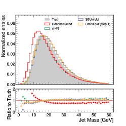
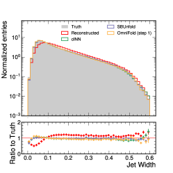
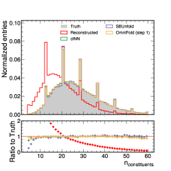
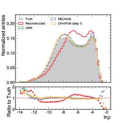
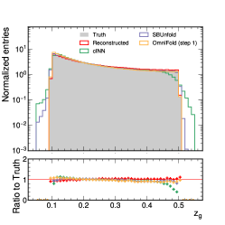
For all distributions we observe significantly lower EMD values for SBUnfold compared to cINN with four out of six also showing lower values of the triangular discriminator. Uncertainties from the EMD calculation are derived from the standard deviation of 100 bootstraps with replacement taken from the unfolded data. We observe the EMD uncertainties from cINN to be often higher than SBUnfold, which points to improved stability from SBUnfold due the more informative prior.

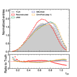
Next, we keep the same unfolding methodology from SBUnfold and cINN trained over Pythia samples but instead use reconstructed events from Herwig as the data representative. We compare the unfolded results between the different distributions in Fig. 3.

We observe improved agreement in all unfolded distributions compared to the distributions of reconstructed events, while systematic shifts are observed in all unfolding methodologies for the jet mass and $\tau_{21}$ distributions. These features highlight the prior dependence of all models which cannot be excluded without the presence of the M step and additional iterations. In Table 2 we calculate the EMD and triangular discriminator using the unfolded distributions with Herwig as pseudo-data.

Table 2: Comparison of the earth mover’s distance (EMD) and triangular discriminator between different algorithms. EMD is calculated over unbinned distributions while triangular discriminator uses histograms as inputs. Uncertainties from EMD are derived using 100 bootstraps with replacement taken from the unfolded data. Results are evaluated using 600,000 pseudo-data points sampled from Herwig. Quantities in bold represent the method with best performance.

Model	EMD($\times 10$)/Triangular Discriminator($\times 10^{3}$)
	OmniFold Step 1	cINN	SBUnfold
Jet mass	6.1$\pm$0.1/1.5	10.1$\pm$1.2/2.4	9.0$\pm$0.1/3.1
Jet Width	0.06$\pm$0.001/1.1	0.05$\pm$0.003/0.7	0.02$\pm$0.001/0.2
N	1.7$\pm$0.1/0.2	6.1$\pm$4.0/0.2	3.0$\pm$0.1/0.6
$\log\rho$	1.35$\pm$0.03/1.1	3.1$\pm$2.1/0.8	0.4$\pm$0.1/0.7
$z_{g}$	0.086$\pm$0.001/1.2	0.3$\pm$0.1/12.7	0.049$\pm$0.001/3.5
$\tau_{21}$	0.23$\pm$0.02/4.6	0.7$\pm$0.4/3.5	0.12$\pm$0.02/1.4

Once again we observe a good performance of SBUnfold, achieving the lowest EMD values for four out of six distributions and lowest triangular discriminator values for three of the six. We also observe OmniFold achieving similar performance for all observables, in particular OmniFold shows improved performance for the particle multiplicity, which is not a continuous distribution and hence harder for generative models to determine precisely. We also study how SBUnfold corrects physics observables back to generator level events by calculating the migration matrix between reconstructed and unfolded observables. Results showing that SBUnfold learns to apply small corrections to reconstructed events are shown in App. B.

OmniFold is also the only algorithm that uses the statistical power of the data to determine the unfolded distributions. We investigate how the unfolding results change when the available number of data entries is reduced to only 1,000 instead of the 600,000 thousands we used previously. For both SBUnfold and cINN this change only modifies the number of generated samples from the trained model while OmniFold only has access to the 1,000 data examples during training while the number of Pythia samples is not changed and kept at 1,000,000. The unfolded results are shown in Fig. 4.

Figure 4: Comparison between different unfolding algorithms for six different physics observables unfolded. All observables are unfolded simultaneously without binning, with histograms shown only for evaluation. Results are evaluated over 1’000 pseudo-data points, the same number was used to train OmniFold while other algorithms only rely on simulation. Statistical uncertainties are shown only in the ratio panel. Pseudo-data is taken from Herwig while Pythia is taken as the main simulator.

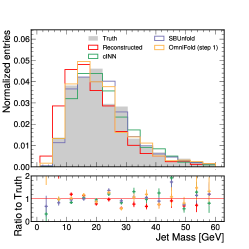
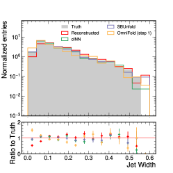
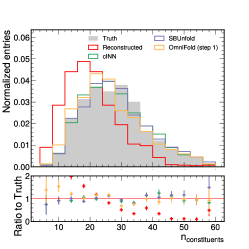
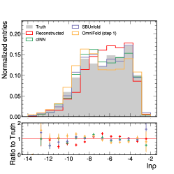
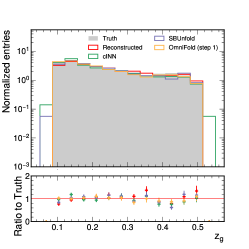
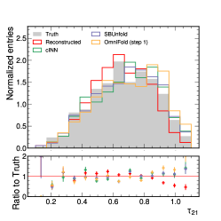
Due to the lower number of data entries we observe larger statistical fluctuations from the unfolded results which still shows a good agreement compared to the expected quantities. We evaluate further the unfolded results by calculating the EMD and triangular discriminator, listed in Table 3.

Table 3: Comparison of the earth mover’s distance (EMD) and triangular discriminator between different algorithms. EMD is calculated over unbinned distributions while triangular discriminator uses histograms as inputs. Uncertainties from EMD are derived using 100 bootstraps with replacement taken from the unfolded data. Results are evaluated using 1’000 pseudo-data points sampled from Herwig. Quantities in bold represent the method with best performance.

Model	EMD($\times 10$)/Triangular Discriminator($\times 10^{3}$)
	OmniFold Step 1	cINN	SBUnfold
Jet mass	8.7$\pm$1.8/13.6	9.2$\pm$3.0/8.4	7.7$\pm$2.5/6.9
Jet Width	0.14$\pm$0.02/18	0.07$\pm$0.02/5.7	0.05$\pm$0.02/4.6
N	12$\pm$3/10.9	5.4$\pm$1.3/3.8	5.8 $\pm$1.6/3.7
$\log\rho$	4.0$\pm$0.8/11	1.6$\pm$0.5/6.2	1.2$\pm$0.3/4.4
$z_{g}$	0.08$\pm$0.02/1.5	0.08$\pm$0.03/7.2	0.06$\pm$0.01/7.1
$\tau_{21}$	0.4$\pm$0.07/16	0.2$\pm$0.05/12	0.1$\pm$0.04/8

The reported results for SBUnfold and cINN are less affected by the reduced data sizes, even though the uncertainties from EMD have greatly increased due to limited pseudo-data examples. On the other hand, OmniFold shows a worse degradation compared to previous results, with EMD values often disagreeing by more than two standard deviations.

V Conclusion and Outlook

In this paper we presented SBUnfold, an unfolding algorithm that uses a Schrödinger bridge (SB) to design a stochastic mapping between distributions. Since the SB allows the transport between arbitrary distributions, SBUnfold does not require a tractable prior similar to other generative models, but instead uses a diffusion process to directly denoise physics observables from detector effects. We have demonstrated the performance of SBUnfold using synthetic $Z$+jets samples and compared with both state-of-the-art methods using generative models (cINN) and reweighting (OmniFold). Using different metrics, we observe an excellent performance of SBUnfold. Compared to cINN, SBUnfold shows improved fidelity for distributions with sharp features and smaller uncertainties overall likely due to more informative priors from reconstructed level events. Compared to OmniFold, SBUnfold shows a more robust performance against variations of the number of available data observations, showing promising results for cases where the amount of available data is reduced.

We have only investigated the expectation step of different unfolding algorithms, leaving the maximization step for future study. We notice that the maximization step based on classifiers used by IcINN is also applicable for SBUnfold, and would be interesting to compare how the unfolding results improve with subsequent iterations between both algorithms.

Finally, similar to OmniFold, SBUnfold can be readily adapted to different data structures such as image-like datasets. On the other hand, the diffusion process currently relies on the specific ordering of the features used during unfolding (see Eq. 8), making the application of SBUnfold with low-level features, such as particles, not trivial. Following studies will investigate how to accommodate permutation invariance within SBUnfold.

Code Availability

The code for this paper can be found at https://github.com/ViniciusMikuni/SBUnfold.

Appendix A Comparison with standard diffusion models

We investigate the benefits of using SBUnfold as opposed to a standard diffusion model. The diffusion model implementation follows the FPCD model proposed in [58] for jet kinematic generation. The backbone neural network architecture used is the same as the one used in SBUnfold. Similarly, the learning rate, number of training epochs, and training samples are kept the same between the two models. The main conceptual difference between the implementations is that SBUnfold starts from the reconstruction level events instead of a Gaussian prior used in FPCD. Similarly to the cINN implementation, the FPCD model is only conditioned on reconstruction level events to determine the unfolded response. Results of the unfolded distributions using Pythia both as pseudo-data and simulation are shown in Fig. 5.

Figure 5: Comparison between different unfolding algorithms for six different physics observables unfolded. Results are evaluated over 600’000 pseudo-data points. Statistical uncertainties are shown only in the ratio panel. Pseudo-data and simulation are described by Pythia.

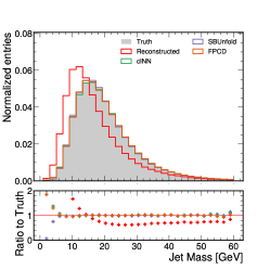
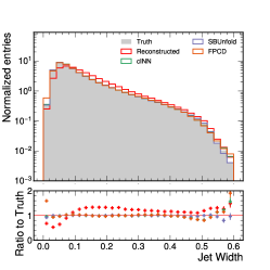
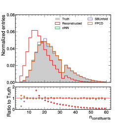
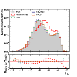
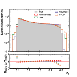
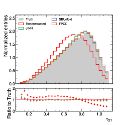
For all distributions we observe a good agreement between the unfolded results and the pseudo-data. In Table 4 we calculate the EMD and triangular discriminator using the unfolded distributions obtained by the different methodologies.

Table 4: Comparison of the earth mover’s distance (EMD) and triangular discriminator between different unfolding methodologies. EMD is calculated over unbinned distributions while triangular discriminator uses histograms as inputs. Uncertainties from EMD are derived using 100 bootstraps with replacement taken from the unfolded data. Results are evaluated using 600’000 pseudo-data points sampled from Pythia. Quantities in bold represent the method with best performance.

Model	EMD($\times 10$)/Triangular Discriminator($\times 10^{3}$)
	FPCD	cINN	SBUnfold
Jet mass	0.74$\pm$0.08/0.19	1.4$\pm$0.2/0.29	0.70$\pm$0.06/0.30
Jet Width	0.0087$\pm$0.0006/0.9	0.013$\pm$0.002/0.25	0.0029$\pm$0.0005/0.04
N	0.81$\pm$0.06/0.1	2.3$\pm$0.8/0.09	0.57$\pm$0.04/0.9
$\log\rho$	0.34$\pm$0.01/0.77	1.1$\pm$0.3/0.64	0.27$\pm$0.01/0.68
$z_{g}$	0.035$\pm$0.007/12.4	0.095$\pm$0.003/10.9	0.009$\pm$0.001/3.1
$\tau_{21}$	0.024$\pm$0.002/0.3	0.2$\pm$0.1/0.6	0.016$\pm$0.001/0.2

From the results we observe that FPCD often outperforms the cINN in the EMD metric while still not achieving the same level of performance as SBUnfold. These results indicate that standard diffusion models may be more expressive compared to the normalizing flow model implemented in the original cINN, but still not as precise as SBUnfold which leverages the more informative prior distribution from reconstruction level objects rather than the Gaussian prior required by both cINN and FPCD.

Appendix B Migration matrix of unfolded events

In this appendix we investigate how SBUnfold maps reconstructed level distributions back to generator level samples by calculating the corresponding migration matrix using Herwig as the pseudo-data while the detector response is derived from the Pythia simulation. The distributions are shown in Fig. 6.

Figure 6: Migration distribution between reconstructed level events and generator level distribution after unfolding with SBUnfold. Results are evaluated over 600’000 pseudo-data points. Pseudo-data is taken from Herwig while Pythia is taken as the main simulator.

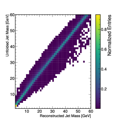
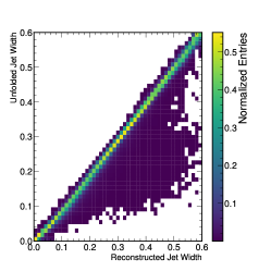
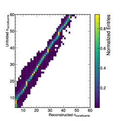
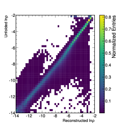
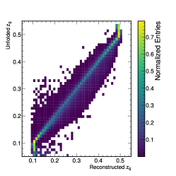
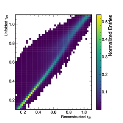
The migration matrix for all observables has a high fraction of events present close to the diagonal, consistent with SBunfold learning to apply only a small correction to the inputs.

References

- Glazov [2017] A. Glazov, (2017), arXiv:1712.01814 [physics.data-an] .
- Datta et al. [2018] K. Datta, D. Kar, and D. Roy, (2018), arXiv:1806.00433 [physics.data-an] .
- Bunse et al. [2018] M. Bunse, N. Piatkowski, T. Ruhe, W. Rhode, and K. Morik, in 5th International Conference on Data Science and Advanced Analytics (DSAA) (IEEE, 2018) pp. 21–30.
- Ruhe et al. [2019] T. Ruhe, T. Voigt, M. Wornowizki, M. Börner, W. Rhode, and K. Morik (2019).
- Andreassen et al. [2020] A. Andreassen, P. T. Komiske, E. M. Metodiev, B. Nachman, and J. Thaler, Phys. Rev. Lett. 124, 182001 (2020), arXiv:1911.09107 [hep-ph] .
- Bellagente et al. [2019] M. Bellagente, A. Butter, G. Kasieczka, T. Plehn, and R. Winterhalder, (2019), 10.21468/SciPostPhys.8.4.070, arXiv:1912.00477 [hep-ph] .
- Bellagente et al. [2020] M. Bellagente, A. Butter, G. Kasieczka, T. Plehn, A. Rousselot, and R. Winterhalder, (2020), 10.21468/SciPostPhys.9.5.074, arXiv:2006.06685 [hep-ph] .
- Vandegar et al. [2020] M. Vandegar, M. Kagan, A. Wehenkel, and G. Louppe, (2020), arXiv:2011.05836 [stat.ML] .
- Andreassen et al. [2021] A. Andreassen, P. T. Komiske, E. M. Metodiev, B. Nachman, A. Suresh, and J. Thaler, (2021), arXiv:2105.04448 [stat.ML] .
- Howard et al. [2022] J. N. Howard, S. Mandt, D. Whiteson, and Y. Yang, Sci. Rep. 12, 7567 (2022), arXiv:2101.08944 [hep-ph] .
- Backes et al. [2022] M. Backes, A. Butter, M. Dunford, and B. Malaescu, (2022), arXiv:2212.08674 [hep-ph] .
- Arratia et al. [2022] M. Arratia, D. Britzger, O. Long, and B. Nachman, JINST 17, P07009 (2022), arXiv:2203.16722 [hep-ex] .
- Chan and Nachman [2023] J. Chan and B. Nachman, Phys. Rev. D 108, 016002 (2023), arXiv:2302.05390 [hep-ph] .
- Shmakov et al. [2023] A. Shmakov, K. Greif, M. Fenton, A. Ghosh, P. Baldi, and D. Whiteson, (2023), arXiv:2305.10399 [hep-ex] .
- Alghamdi et al. [2023] T. Alghamdi et al., (2023), arXiv:2307.04450 [hep-ph] .
- Arratia et al. [2021] M. Arratia et al., (2021), arXiv:2109.13243 [hep-ph] .
- Andreev et al. [2022] V. Andreev et al. (H1), Phys. Rev. Lett. 128, 132002 (2022), arXiv:2108.12376 [hep-ex] .
- H1 Collaboration [2022] H1 Collaboration, H1prelim-22-031 (2022).
- Andreev et al. [2023] V. Andreev et al. (H1), (2023), arXiv:2303.13620 [hep-ex] .
- H1 Collaboration [2023] H1 Collaboration, H1prelim-23-031 (2023).
- LHC [2022] (2022), arXiv:2208.11691 [hep-ex] .
- Komiske et al. [2022] P. T. Komiske, S. Kryhin, and J. Thaler, Phys. Rev. D 106, 094021 (2022), arXiv:2205.04459 [hep-ph] .
- Song [2023] Y. Song (STAR), (2023), arXiv:2307.07718 [nucl-ex] .
- Lucy [1974] L. B. Lucy, Astronomical Journal 79, 745 (1974).
- Richardson [1972] W. H. Richardson, J. Opt. Soc. Am. 62, 55 (1972).
- D’Agostini [1995] G. D’Agostini, Nucl. Instrum. Meth. A362, 487 (1995).
- Rezende and Mohamed [2016] D. J. Rezende and S. Mohamed, Proceedings of Machine Learning Research, 37, 1530 (2016), arXiv:1505.05770 [stat.ML] .
- Goodfellow et al. [2014] I. J. Goodfellow, J. Pouget-Abadie, M. Mirza, B. Xu, D. Warde-Farley, S. Ozair, A. Courville, and Y. Bengio, (2014), arXiv:1406.2661 [stat.ML] .
- Song et al. [2021] Y. Song, J. Sohl-Dickstein, D. P. Kingma, A. Kumar, S. Ermon, and B. Poole, ArXiv abs/2011.13456 (2021).
- Schrödinger [1931] E. Schrödinger, Sitzungsberichte der Preuss Akad. Wissen. Phys. Math. Klasse Sonderausgabe 9, 144 (1931).
- Liu et al. [2023] G.-H. Liu, A. Vahdat, D.-A. Huang, E. A. Theodorou, W. Nie, and A. Anandkumar, arXiv preprint arXiv:2302.05872 (2023).
- Ho et al. [2020] J. Ho, A. Jain, and P. Abbeel, in Advances in Neural Information Processing Systems, Vol. 33, edited by H. Larochelle, M. Ranzato, R. Hadsell, M. Balcan, and H. Lin (Curran Associates, Inc., 2020) pp. 6840–6851.
- Peyré et al. [2019] G. Peyré, M. Cuturi, et al., Foundations and Trends® in Machine Learning 11, 355 (2019).
- Andreassen et al. [2019] A. Andreassen, P. Komiske, E. Metodiev, B. Nachman, and J. Thaler, “Pythia/Herwig + Delphes Jet Datasets for OmniFold Unfolding,” (2019).
- Bahr et al. [2008] M. Bahr et al., Eur. Phys. J. C58, 639 (2008), arXiv:0803.0883 [hep-ph] .
- Bellm et al. [2016] J. Bellm et al., Eur. Phys. J. C76, 196 (2016), arXiv:1512.01178 [hep-ph] .
- Bellm et al. [2017] J. Bellm et al., (2017), arXiv:1705.06919 [hep-ph] .
- ATL [2014] ATLAS Run 1 Pythia8 tunes, Tech. Rep. ATL-PHYS-PUB-2014-021 (CERN, Geneva, 2014).
- Sjöstrand et al. [2008] T. Sjöstrand, S. Mrenna, and P. Z. Skands, Comput. Phys. Commun. 178, 852 (2008), arXiv:0710.3820 [hep-ph] .
- Sjöstrand et al. [2006] T. Sjöstrand, S. Mrenna, and P. Z. Skands, JHEP 05, 026 (2006), arXiv:hep-ph/0603175 [hep-ph] .
- Sjöstrand et al. [2015] T. Sjöstrand, S. Ask, J. R. Christiansen, R. Corke, N. Desai, P. Ilten, S. Mrenna, S. Prestel, C. O. Rasmussen, and P. Z. Skands, Comput. Phys. Commun. 191, 159 (2015), arXiv:1410.3012 [hep-ph] .
- de Favereau et al. [2014] J. de Favereau, C. Delaere, P. Demin, A. Giammanco, V. Lemaître, A. Mertens, and M. Selvaggi (DELPHES 3), JHEP 02, 057 (2014), arXiv:1307.6346 [hep-ex] .
- Cacciari et al. [2008] M. Cacciari, G. P. Salam, and G. Soyez, JHEP 04, 063 (2008), arXiv:0802.1189 [hep-ph] .
- Cacciari et al. [2012] M. Cacciari, G. P. Salam, and G. Soyez, Eur. Phys. J. C72, 1896 (2012), arXiv:1111.6097 [hep-ph] .
- Cacciari and Salam [2006] M. Cacciari and G. P. Salam, Phys. Lett. B641, 57 (2006), arXiv:hep-ph/0512210 [hep-ph] .
- Thaler and Van Tilburg [2011] J. Thaler and K. Van Tilburg, JHEP 03, 015 (2011), arXiv:1011.2268 [hep-ph] .
- Thaler and Van Tilburg [2012] J. Thaler and K. Van Tilburg, JHEP 02, 093 (2012), arXiv:1108.2701 [hep-ph] .
- Larkoski et al. [2014] A. J. Larkoski, S. Marzani, G. Soyez, and J. Thaler, JHEP 05, 146 (2014), arXiv:1402.2657 [hep-ph] .
- Dasgupta et al. [2013] M. Dasgupta, A. Fregoso, S. Marzani, and G. P. Salam, JHEP 09, 029 (2013), arXiv:1307.0007 [hep-ph] .
- [50] “Fastjet contrib,” https://fastjet.hepforge.org/contrib/.
- He et al. [2016] K. He, X. Zhang, S. Ren, and J. Sun, in Proceedings of the IEEE conference on computer vision and pattern recognition (2016) pp. 770–778.
- Xu et al. [2015] B. Xu, N. Wang, T. Chen, and M. Li, CoRR abs/1505.00853 (2015), 1505.00853 .
- Paszke et al. [2019] A. Paszke, S. Gross, F. Massa, A. Lerer, J. Bradbury, G. Chanan, T. Killeen, Z. Lin, N. Gimelshein, L. Antiga, et al., Advances in neural information processing systems 32 (2019).
- Abadi et al. [2016] M. Abadi, P. Barham, J. Chen, Z. Chen, A. Davis, J. Dean, M. Devin, S. Ghemawat, G. Irving, M. Isard, et al., in OSDI, Vol. 16 (2016) pp. 265–283.
- Topsoe [2000] F. Topsoe, IEEE Transactions on Information Theory 46, 1602 (2000).
- Gras et al. [2017] P. Gras, S. Höche, D. Kar, A. Larkoski, L. Lönnblad, S. Plätzer, A. Siódmok, P. Skands, G. Soyez, and J. Thaler, JHEP 07, 091 (2017), arXiv:1704.03878 [hep-ph] .
- Bright-Thonney and Nachman [2019] S. Bright-Thonney and B. Nachman, JHEP 03, 098 (2019), arXiv:1810.05653 [hep-ph] .
- Mikuni et al. [2023] V. Mikuni, B. Nachman, and M. Pettee, Phys. Rev. D 108, 036025 (2023).