Understanding Dark Scenes by Contrasting Multi-Modal Observations

Abstract

Understanding dark scenes based on multi-modal image data is challenging, as both the visible and auxiliary modalities provide limited semantic information for the task. Previous methods focus on fusing the two modalities but neglect the correlations among semantic classes when minimizing losses to align pixels with labels, resulting in inaccurate class predictions. To address these issues, we introduce a supervised multi-modal contrastive learning approach to increase the semantic discriminability of the learned multi-modal feature spaces by jointly performing cross-modal and intra-modal contrast under the supervision of the class correlations. The cross-modal contrast encourages same-class embeddings from across the two modalities to be closer and pushes different-class ones apart. The intra-modal contrast forces same-class or different-class embeddings within each modality to be together or apart. We validate our approach on a variety of tasks that cover diverse light conditions and image modalities. Experiments show that our approach can effectively enhance dark scene understanding based on multi-modal images with limited semantics by shaping semantic-discriminative feature spaces. Comparisons with previous methods demonstrate our state-of-the-art performance. Code and pretrained models are available at https://github.com/palmdong/SMMCL.

1 Introduction

(a) RGB

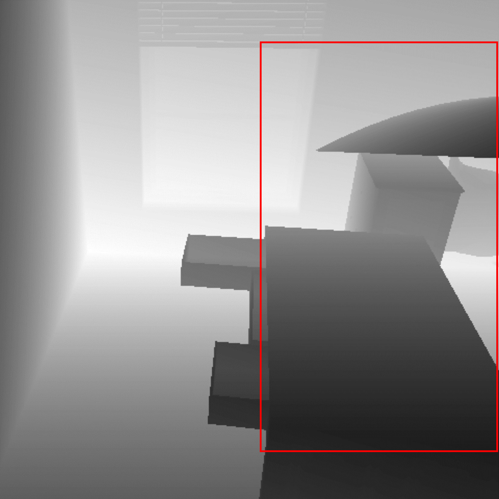
(b) Depth

(c) Ground Truth

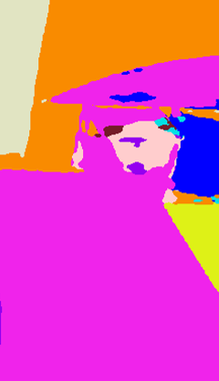
(d) CEN [55]

(e) ToFusion [53]

(f) Ours

Figure 1: Low-light indoor scene segmentation from RGB-depth data. Compared to state-of-the-art methods, our model with supervised multi-modal contrastive learning achieves higher accuracy.

A robust scene understanding capability in dark environments, including low-light indoor and nighttime outdoor environments, is important to automated work systems such as indoor robots and automotive vehicles [13, 44]. However, semantic segmentation on dark scenes, especially based on observation images from visible RGB modality, is not trivial due to the poor visibility of spatial content in images caused by adverse light conditions [12, 15].

Combining images from multiple modalities that can provide complementary spatial information for a scene, often visible RGB modality and an auxiliary depth or thermal modality, has been proved beneficial to semantic segmentation tasks [41, 23]. And numerous multi-modal image semantic segmentation methods have been developed [53, 55, 69, 4, 10, 75, 49].

However, in the task of dark scene segmentation, the visible and auxiliary modalities both provide limited semantic information. To be specific: The visible modality reflects contextual semantic cues in RGB color space, but available cues are usually limited due to its dark nature [15]. The auxiliary modality is robust to adverse lights and can provide rich geometry cues for dark environments, but is lacking in contextual semantics [4, 10]. These cause low discrimination between different semantic classes, as shown in Fig. 1. Previous multi-modal image segmentation methods [66, 53, 55, 69, 4, 10] focus on developing fusion techniques to combine the two modalities, then minimizing cross-entropy losses to align pixels with corresponding labels without considering the correlations (similarities and differences) among semantic classes. As a result, they tend to predict inaccurate class information for objects in darkness (Fig. 1). Overall, multi-modal dark scene understanding remains an open problem.

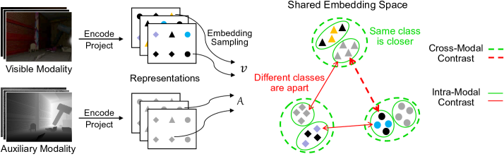
Figure 2: An illustration of our supervised multi-modal contrastive learning approach. During training, embeddings from the visible and auxiliary modalities are cast to a shared space, where cross-modal and intra-modal contrast are jointly performed under the supervision of the class correlations. Same shape means the embeddings are from the same semantic class and are positive to each other. Colored, black, and grey mean the embeddings carry semantic cues, are not observable, and lack contextual semantics, respectively.

In this paper, we address the issues by increasing the semantic discriminability of the learned feature spaces via contrastive learning. Specifically, we introduce a supervised multi-modal contrastive learning approach (Fig. 2) to boost the learning on the visible and auxiliary modalities and encourage them to be semantic-discriminative, by jointly performing cross-modal and intra-modal contrast under the supervision of the class correlations. The cross-modal contrast encourages same-class embeddings from across the two modalities to be closer and simultaneously pushes different-class ones apart. Within each modality, the intra-modal contrast pulls together embeddings from the same class and forces apart those from different classes. By regularizing the embeddings with considering the class similarities and differences, the encoder feature spaces learned from the two modalities can show higher semantic discriminability. With the adoption of our approach, our segmentation model achieves much higher accuracy when understanding dark scenes based on multi-modal images with limited semantics (Fig. 1).

Contributions: (1) We tackle dark scene understanding from a new perspective by contrasting multi-modal images with limited semantics. (2) We introduce the first supervised multi-modal contrastive learning approach for image segmentation, and show it can effectively enhance dark scene understanding by shaping semantic-discriminative feature spaces. (3) We validate our approach on low-light, nighttime, and normal-light conditions, indoor and outdoor scenes, and RGB, depth, and thermal modalities, demonstrating its effectiveness, generalizability, and applicability. (4) We compare our model and approach with state-of-the-art methods on different tasks, showing our superiority quantitatively and qualitatively.

2 Related Work

2.1 Semantic Segmentation

Semantic segmentation is the task of understanding scenes by assigning each pixel in an image to a specific class. Since FCN [34] was proposed, numerous CNN-based semantic segmentation methods have been developed. Representative work includes the DeepLab series [5, 6, 7], multi-scale networks [70, 43, 50], boundary or context-aware networks [3, 16, 73, 64, 77, 62], and attention-based networks [71, 17, 74, 27]. Most recently, Vision Transformers [11, 30, 21, 58, 63, 42] have shown great potential and outperformed CNN-based methods. However, these advances are made for normal-light scenarios. In practical applications, there is a need for a robust scene understanding capability in dark environments.

2.2 Dark Scene Semantic Segmentation

Existing dark scene semantic segmentation methods are mainly developed based on visible RGB data, and can be divided into unsupervised domain adaptation methods and supervised methods. Unsupervised domain adaptation methods [20, 19, 56, 40, 39, 14] tackle unlabeled dark scenes by transferring knowledge from labeled normal-light scenes that share similar spatial content. The problems with such methods are that they require paired dark-normal training data, which is hard to collect in practice, and their unsupervised working piepline causes limited performance [15, 28]. Supervised methods [15, 32, 59, 46, 67, 68] learn the task from labeled dark scene data directly, and so avoid the need for additional normal-light data. However, they still show unsatisfactory performance on regions of poor visibility because reliable contextual cues in the visible modality is limited [15, 66]. Therefore, recent methods [28, 66, 69, 37] combine auxiliary modalities that can provide robust geometry cues for even dark environments.

2.3 Multi-Modal Image Semantic Segmentation

Multi-modal image data, e.g., RGB-depth and RGB-thermal, has been proven beneficial to semantic segmentation due to the capability of providing complementary spatial information for scenes. Numerous methods with advanced fusion techniques, such as token fusion [53], channel exchanging [55, 54], feature interaction modules [69, 66, 10, 75, 61], and novel convolutions [4, 60, 51, 8], have been developed and show promising performance, especially for normal-light scenes. On dark scenes, however, they still suffer inaccurate class predictions because: (1) The visible and auxiliary modalities both provide limited semantic information, which causes low discrimination between different classes. (2) They neglect the correlations among classes when minimizing losses to align pixels with labels. To address the issues, we introduce a supervised multi-modal contrastive learning approach to increase the semantic discriminability of the learned feature spaces of the two modalities, by regularizing their embeddings under the supervision of the class correlations. We demonstrate that our approach enables a higher accuracy in understanding dark scenes and also generalizes well to normal-light scenes.

2.4 Contrastive Learning

The idea of self-supervised contrastive learning [24, 57, 25, 9] is to pull an anchor closer to a positive sample in embedding space and further from many negative samples, without knowing their labels. Supervised contrastive learning [29] leverages label information to align embeddings and directly consider positive samples from the same class and negative classes from different classes. The use of a supervised paradigm enables better generalization in general image classification and segmentation tasks [29, 38, 2, 72, 26, 52].

In the field of multi-modal learning, various self-supervised contrastive techniques [1, 78, 65, 18, 36, 33] have been presented. We introduce a supervised multi-modal learning approach to tackle dark scene understanding. Unlike those self-supervised contrastive techniques [18, 36, 33], which need to generate positive and/or negative samples via complicated augmentation, our supervised paradigm effectively aligns multi-modal embeddings by leveraging available class labels. This allows to directly and fully exploit the class correlations and the correspondence between cross-modal contextual and geometry cues. We demonstrate the effectiveness and superiority of our approach with comprehensive ablations and comparisons.

3 Method

We first give an overview of our model, then detail our supervised multi-modal contrastive learning approach.

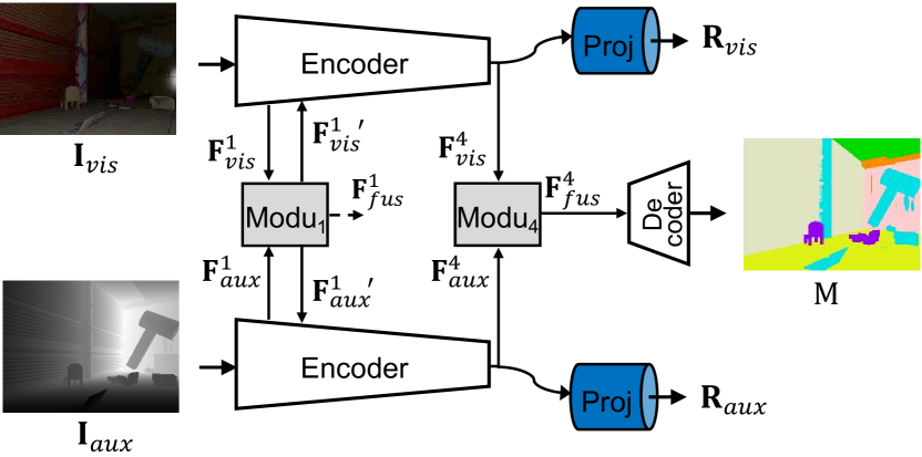
Figure 3: An illustration of our segmentation model. Final features from the encoders are mapped to representations by the projectors. The representations are further utilized to generate embeddings in our supervised multi-modal contrastive learning approach.

3.1 Model Overview

Our model is illustrated in Fig. 3. Given a dark scene image $\textbf{I}_{vis}\in\mathbb{R}^{H\times W\times 3}$ in visible modality and its counterpart $\textbf{I}_{aux}\in\mathbb{R}^{H\times W}$ from an auxiliary modality, we use two encoders to encode them and extract multi-modal features $\textbf{F}_{vis}^{m}\in~{}\mathbb{R}^{h\times w\times c}$ and $\textbf{F}_{aux}^{m}\in~{}\mathbb{R}^{h\times w\times c}$, where $m$ = 1, 2, 3, 4 corresponds to the stage in the encoders. Intermediate modules are developed to further process the features.

In each module, as illustrated in Fig. 4, we learn a shared spatial coefficient matrix $\textbf{S}_{m}\in\mathbb{R}^{h\times w}$ and a shared channel coefficient vector $\textbf{c}_{m}\in~{}\mathbb{R}^{c}$ from the input feature pair $\textbf{F}_{vis}^{m}$ and $\textbf{F}_{aux}^{m}$ to model the dependency between the visible and auxiliary modalities at spatial and channel dimensions. Then, to facilitate the information interaction between the two modalities, $\textbf{F}_{vis}^{m}$ and $\textbf{F}_{aux}^{m}$ are updated as:

$${\textbf{F}^{m}_{vis}}^{\prime}=\textbf{F}_{vis}^{m}+\textbf{S}_{m}\ast\textbf{F}_{aux}^{m}+\textbf{c}_{m}\circledast\textbf{F}_{aux}^{m},$$ (1)

$${\textbf{F}^{m}_{aux}}^{\prime}=\textbf{F}_{aux}^{m}+\textbf{S}_{m}\ast\textbf{F}_{vis}^{m}+\textbf{c}_{m}\circledast\textbf{F}_{vis}^{m},$$ (2)

where $\ast$ and $\circledast$ denote spatial and channel-wise multiplication, respectively. ${\textbf{F}^{m}_{vis}}^{\prime}\in\mathbb{R}^{h\times w\times c}$ and ${\textbf{F}^{m}_{aux}}^{\prime}\in\mathbb{R}^{h\times w\times c}$ are then fed to the next stage in the encoders. Additionally, a fusion feature $\textbf{F}^{m}_{fus}\in\mathbb{R}^{h\times w\times c}$ is produced by fusing ${\textbf{F}^{m}_{vis}}^{\prime}$ and ${\textbf{F}^{m}_{aux}}^{\prime}$ via a $1\times 1$ convolution.

The decoder predicts a segmentation mask ${\rm M}\in~{}\mathbb{R}^{H\times W}$ based on fusion features from the four modules. During training, the prediction of ${\rm M}$ is supervised by a ground-truth label ${\rm L}\in~{}\mathbb{R}^{H\times W}$ via a cross-entropy loss $\mathcal{L}_{ce}({\rm M},{\rm L})$.

Two projectors, following the encoders, map final features $\textbf{F}_{vis}^{4}$ and $\textbf{F}_{aux}^{4}$ to representations $\textbf{R}_{vis}\in\mathbb{R}^{h\times w\times d}$ and $\textbf{R}_{aux}\in~{}\mathbb{R}^{h\times w\times d}$, respectively, which are utilized to generate embeddings in our supervised multi-modal contrastive learning approach. Detailed structure settings of the intermediate modules and the projectors are provided in Sec. 4.1.

3.2 Supervised Multi-Modal Contrastive Learning

Multi-modal dark scene understanding is challenging because the visible and auxiliary modalities both provide limited semantics. We address this issue by introducing a supervised multi-modal contrastive learning approach (Fig. 2) to encourage the encoder feature spaces learned from the two modalities to be semantic-discriminative.

Embedding Generation. To a set of visible-auxiliary representation pairs $\{\textbf{R}_{vis}^{b},\textbf{R}_{aux}^{b}\in\mathbb{R}^{h\times w\times d}\}_{b=1}^{B}$ learned from a training batch $B$ of input image pairs and a set of corresponding labels $\{\widetilde{\rm L}^{b}\in~{}\mathbb{R}^{h\times w}\}_{b=1}^{B}$ generated by downscaling the ground-truth labels, we sample a visible embedding set $\mathcal{V}=\{\textbf{{v}}_{i}\in\mathbb{R}^{d}:\textbf{{v}}_{i}\to\widetilde{\rm L}_{\textbf{{v}}_{i}}\}$ and an auxiliary embedding set $\mathcal{A}=\{\textbf{{a}}_{j}\in\mathbb{R}^{d}:\textbf{{a}}_{j}\to\widetilde{\rm L}_{\textbf{{a}}_{j}}\}$ from the representations. Taking visible embedding $\textbf{{v}}_{i}$ as an example, $i$ denotes that it is sampled at the $i$-th spatial position in a visible representation, and $\widetilde{\rm L}_{\textbf{{v}}_{i}}$ is its class label, which is obtained at the $i$-th position from the corresponding label and is utilized to measure its class correlation with other embeddings. In both modalities, we randomly sample $n$ embeddings per instance from each class present in the batch, and set $n$ as the number of pixels from the class with the least occurrences, following the protocol in [38]. This setting maintains a balance for embeddings from each present class. Then, $\mathcal{V}$ and $\mathcal{A}$ are cast to a shared space to perform contrast under the supervision of the class correlations: Embeddings with the same label (or different labels) are same-class (or different-class) and are aligned as positive (or negative) samples.

Cross-Modal Contrast. The cross-modal contrast is to shape the visible and auxiliary feature spaces by considering the cross-modal context-geometry correspondence. To this end, we encourage embeddings from one modality to be closer to the same-class embeddings from the other modality and push apart different-class ones from across the two modalities by minimizing a cross-modal contrastive loss:

$$\mathcal{L}_{cm}(\mathcal{V},\mathcal{A})=\frac{1}{\mid\mathcal{V}\mid}\sum_{\textbf{{v}}_{i}\in\mathcal{V}}\frac{1}{\mid\mathcal{P}_{\textbf{{v}}_{i}}\mid}\sum_{\textbf{{a}}^{+}\in\mathcal{P}_{\textbf{{v}}_{i}}}\mathcal{L}_{\rm NCE}(\textbf{{v}}_{i},\textbf{{a}}^{+}),$$ (3)

where

$$\begin{split}\begin{aligned} &\mathcal{L}_{\rm NCE}(\textbf{{v}}_{i},\textbf{{a}}^{+})=\\ &-{\rm log}\frac{{\rm exp}(\textbf{{v}}_{i}\cdot\textbf{{a}}^{+}/\tau)}{{\rm exp}(\textbf{{v}}_{i}\cdot\textbf{{a}}^{+}/\tau)+\sum_{\textbf{{a}}^{-}\in\mathcal{N}_{\textbf{{v}}_{i}}}{\rm exp}(\textbf{{v}}_{i}\cdot\textbf{{a}}^{-}/\tau)}\end{aligned}\end{split}$$ (4)

is the InfoNCE loss [47]. The symbol $\cdot$ denotes the dot product. $\tau$ is a temperature hyperparameter. $\mathcal{P}_{\textbf{{v}}_{i}}=\{\textbf{{a}}_{j}\in\mathcal{A}:j\neq i,\widetilde{\rm L}_{\textbf{{a}}_{j}}=\widetilde{\rm L}_{\textbf{{v}}_{i}}\}$ and $\mathcal{N}_{\textbf{{v}}_{i}}=\{\textbf{{a}}_{j}\in\mathcal{A}:j\neq i,\widetilde{\rm L}_{\textbf{{a}}_{j}}\neq\widetilde{\rm L}_{\textbf{{v}}_{i}}\}$ are respectively the sets of same-class and different-class auxiliary embeddings, i.e., positive and negative samples, for visible embedding $\textbf{{v}}_{i}$. Note that, since the positive and negative relation among the embeddings is bidirectional, the cross-modal contrast has only one loss term.

Figure 4: The spatial and channel coefficient learning in our intermediate modules. $\textbf{F}_{vis}^{m}$ and $\textbf{F}_{aux}^{m}$ are concatenated along the channel dimension. $\textbf{s}_{m}$ is learned by passing the concatenation to a three-layer MLP and a sigmoid function. $\textbf{c}_{m}$ is learned by first taking global max pooling and average pooling to the concatenation and then passing to a three-layer MLP and sigmoid.

(a) RGB

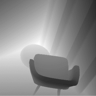
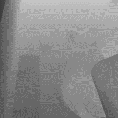
(b) Depth

(c) Ground Truth

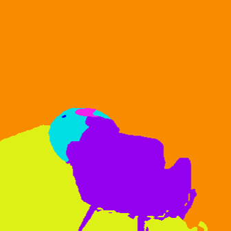
(d) TokenFusion [53]

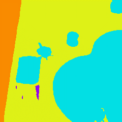
(e) CMX [66]

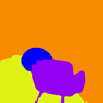
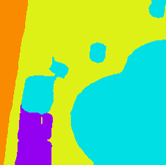
(f) Ours

Figure 5: Low-light indoor scene segmentation from RGB-depth data. Visual comparisons between Base and Ours are provided in Sec. 4.5 and the supplementary material.

Intra-Modal Contrast. The intra-modal contrast shapes the encoder feature spaces of the two modalities by regularizing embeddings within each modality separately. Within the visible modality, same-class or different-class embeddings are pulled closer or pushed apart by minimizing an intra-modal contrastive loss:

$$\mathcal{L}_{vis}(\mathcal{V})=\frac{1}{\mid\mathcal{V}\mid}\sum_{\textbf{{v}}_{i}\in\mathcal{V}}\frac{1}{\mid\mathcal{P}^{\prime}_{\textbf{{v}}_{i}}\mid}\sum_{\textbf{{v}}^{+}\in\mathcal{P}^{\prime}_{\textbf{{v}}_{i}}}\mathcal{L}_{\rm NCE}(\textbf{{v}}_{i},\textbf{{v}}^{+}),$$ (5)

where

$$\begin{split}\begin{aligned} &\mathcal{L}_{\rm NCE}(\textbf{{v}}_{i},\textbf{{v}}^{+})=\\ &-{\rm log}\frac{{\rm exp}(\textbf{{v}}_{i}\cdot\textbf{{v}}^{+}/\tau)}{{\rm exp}(\textbf{{v}}_{i}\cdot\textbf{{v}}^{+}/\tau)+\sum_{\textbf{{v}}^{-}\in\mathcal{N}^{\prime}_{\textbf{{v}}_{i}}}{\rm exp}(\textbf{{v}}_{i}\cdot\textbf{{v}}^{-}/\tau)}.\end{aligned}\end{split}$$ (6)

$\mathcal{P}^{\prime}_{\textbf{{v}}_{i}}=\{\textbf{{v}}_{p}\in\mathcal{V}\mid p\neq i,\widetilde{\rm L}_{\textbf{{v}}_{p}}=\widetilde{\rm L}_{\textbf{{v}}_{i}}\}$ and $\mathcal{N}^{\prime}_{\textbf{{v}}_{i}}=\{\textbf{{v}}_{p}\in\mathcal{V}\mid p\neq i,\widetilde{\rm L}_{\textbf{{v}}_{p}}\neq\widetilde{\rm L}_{\textbf{{v}}_{i}}\}$ are respectively the intra-modal sets of positive and negative samples for $\textbf{{v}}_{i}$. The contrastive loss for the auxiliary modality, i.e., $\mathcal{L}_{aux}(\mathcal{A})$, is similar to Eq. 5. For $\textbf{{a}}_{j}\in\mathcal{A}$, the positive and negative sample sets are $\mathcal{P}^{\prime}_{\textbf{{a}}_{j}}=\{\textbf{{a}}_{q}\in\mathcal{A}\mid q\neq j,\widetilde{\rm L}_{\textbf{{a}}_{q}}=\widetilde{\rm L}_{\textbf{{a}}_{j}}\}$ and $\mathcal{N}^{\prime}_{\textbf{{a}}_{j}}=\{\textbf{{a}}_{q}\in\mathcal{A}\mid q\neq j,\widetilde{\rm L}_{\textbf{{a}}_{q}}\neq\widetilde{\rm L}_{\textbf{{a}}_{j}}\}$, respectively.

Combining the cross-modal contrastive loss and the intra-modal contrastive losses, our full training objective is:

$$\mathcal{L}=\mathcal{L}_{ce}+\lambda_{cm}\mathcal{L}_{cm}+\lambda_{vis}\mathcal{L}_{vis}+\lambda_{aux}\mathcal{L}_{aux}.$$ (7)

Experiments in Sec. 4 show that our approach can effectively enhance dark scene understanding by shaping semantic-discriminative feature spaces.

4 Experiments

4.1 Implementation Details

Network Structure. We employ three different backbones, including ResNet-101, SegFomrer-B2 [58], and SegNext-B [21], to build our segmentation network. The channel setting to the four encoder stages is $[c_{1},c_{2},c_{3},c_{4}]=[64,128,320,512]$. Taking the first of the four intermediate modules as an example, the input and output channel setting of the MLP layers for spatial and channel coefficient learning is listed in Tab. 1, and the input and output channels of the $1\times 1$ convolution used for feature fusion are set as $[2c_{1},c_{1}]$. The two projectors each consist of a two-layer MLP and a linear mapping with $d=256$, where the input and output channels of the MLP layers are equal to $c_{4}$.

	Layer1	Layer2	Layer3
Spatial	$[2c_{1},2c_{1}]$	$[2c_{1},2c_{1}]$	$[2c_{1},1]$
Channel	$[4c_{1},4c_{1}]$	$[4c_{1},4c_{1}]$	$[4c_{1},c_{1}]$

Table 1: Channel setting, $[in,out]$, of the MLP layers for spatial and channel coefficient learning in the first intermediate module.

Contrastive Losses. The weights $\lambda_{cm}$, $\lambda_{vis}$, and $\lambda_{aux}$ in Eq. 7 are set as 0.2 in experiments for low-light indoor scene segmentation, and are set as 0.05 in experiments for nighttime outdoor scene and normal-light scene segmentation. The temperature $\tau$ in $\mathcal{L}_{cm}$, $\mathcal{L}_{vis}$, and $\mathcal{L}_{aux}$ is set as 0.1 in all experiments. Ablations on $\lambda_{cm}$, $\lambda_{vis}$, $\lambda_{aux}$, and $\tau$ are provided in the supplementary material.

(a) RGB

(b) Thermal

(c) Ground Truth

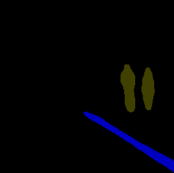
(d) TokenFusion [53]

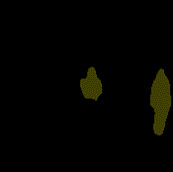
(e) CMX [66]

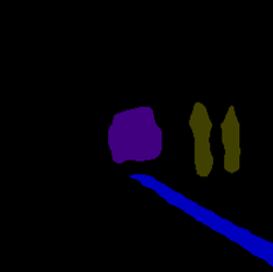
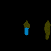
(f) Ours

Figure 6: Nighttime outdoor scene segmentation from RGB-thermal data.

Method	Backbone	mIoU (%)
SA-Gate† [10]	ResNet-101	61.79
ShapeConv†§ [4]	ResNeXt-101	63.26
CEN† [55]	ResNet-101	62.15
TokenFusion† [53]	SegFormer-B2	64.75
CMX† [66]	SegFormer-B2	66.52
Base (w/o SMMCL)	ResNet-101	62.73
	SegFormer-B2	65.69
	SegNeXt-B	66.02
Ours (w SMMCL)	ResNet-101	64.40
	SegFormer-B2	67.77
	SegNeXt-B	68.76

Table 2: Low-light indoor scene segmentation from RGB-depth data. Single-scale results are reported by default. ^†Our implementation. ^§Multi-scale results. The best result is shown in bold.

Training and Evaluation. We implement our model with PyTorch on four Tesla V100 GPUs. During training, we minimize the objective in Eq. 7. The encoders are initialized with the ImageNet-1K pretrained weights. We employ AdamW [35] optimizer. The initial learning rate is $6e^{-5}$ and decays following the poly policy. We use basic augmentation techniques, including random horizontal flipping and random scaling from 0.5 to 1.75. The batch size is 16. We adopt the above training setting in all experiments. In low-light, nighttime, and normal-light scene segmentation tasks, we train our model for 500, 300, and 600 epochs, respectively. During evaluation, we use mean Intersection over Union (mIoU) as the metric. We do not use any tricks, e.g., multi-scale inference, when evaluating our model.

4.2 Validation on Low-Light Indoor Scenes

Dataset and Comparison Methods. We conduct the task of understanding low-light indoor scenes from RGB-depth data on the LLRGBD-synthetic dataset [67]. LLRGBD-synthetic is a large-scale synthetic dataset with 13 semantic classes. To lower data redundancy, we randomly sample 1418 scenes from its training set for training, and sample 479 scenes from its validation set for evaluation. We compare our model with five state-of-the-art multi-modal image segmentation methods: CMX [66], TokenFusion [53], CEN [55], ShapeConv [4], and SA-Gate [10].

Results. Quantitative comparison results are reported in Tab. 2. As can be observed, in low-light indoor scenes, our model trained with the proposed supervised multi-modal contrastive learning approach achieves segmentation accuracy of $68.76\%/67.77\%/64.40\%$, and results in a $2.74\%/2.08\%/1.67\%$ improvement over the baseline. Besides, in comparison with the five state-of-the-art methods, our model achieves the highest accuracy, and outperforms them by a large margin. Figure 5 shows segmentation masks predicted by CMX, TokenFusion, and our best model. Due to a lack of consideration for the class correlations, CMX and TokenFusion tend to predict incorrect class information in the scenes, where the poor visibility in the RGB modality and the lack of contextual semantics of the depth modality cause low class discrimination. By contrast, our model can segment the scenes with much higher accuracy. This is because our supervised multi-modal contrastive learning approach fully considers the correlations among semantic classes, and can effectively enhance multi-modal dark scene understanding by shaping semantic-discriminative feature spaces. We provide comprehensive ablation supports in Sec. 4.5.

Method	Backbone	mIoU (%)
RTFNet [45]	ResNet-152	54.8
GMNet [76]	ResNet-50	57.7
ABMDRNet [69]	ResNet-50	55.5
LASNet [31]	ResNet-152	58.7
TokenFusion† [53]	SegFormer-B2	58.7
CMX [66]	SegFormer-B2	57.8
Base (w/o SMMCL)	ResNet-101	57.2
	SegFormer-B2	57.9
	SegNeXt-B	58.4
Ours (w SMMCL)	ResNet-101	58.9
	SegFormer-B2	59.8
	SegNeXt-B	60.0

Table 3: Nighttime outdoor scene segmentation on RGB-thermal data. Single-scale results are reported. ^†Our implementation. The best result is shown in bold.

(a) RGB

(b) HHA

(c) Ground Truth

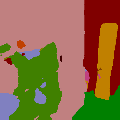
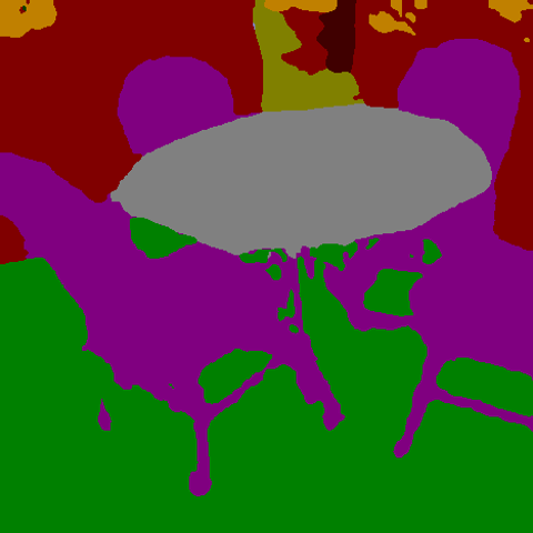
(d) TokenFusion [53]

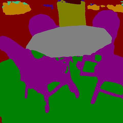
(e) CMX [66]

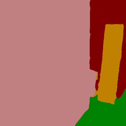
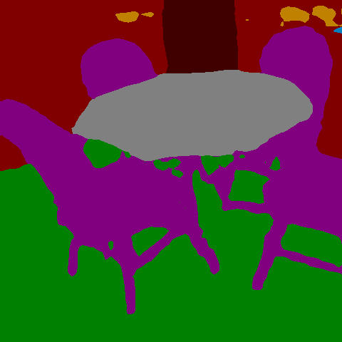
(f) Ours

Figure 7: Normal-light scene segmentation from RGB-depth data. Depth images are encoded to HHA maps [22] in this task.

4.3 Validation on Nighttime Outdoor Scenes

Dataset and Comparison Methods. We further validate our method on real-world nighttime outdoor scenes using RGB-thermal data from the MFNet dataset [23]. MFNet provides 1569 outdoor scenes covering daytime and nighttime, with 9 semantic classes. We train our model with all 784 scenes in the training set and evaluate it on the 188 nighttime scenes in the test set. We compare our model with TokenFusion [53] and five state-of-the-art RGB-thermal segmentation methods: CMX [66], ABMDRNet [69], LASNet [31], GMNet [76], and RTFNet [45].

Results. Table 3 reports the quantitative comparison results. In nighttime outdoor scenes, our model with supervised multi-modal contrastive learning achieves the highest accuracy of $60.0\%/59.8\%/58.9\%$, and gains a $1.6\%/1.9\%/1.7\%$ improvement over the baseline. Moreover, our best model outperforms the second best method, TokenFusion, by $1.3\%$. Figure 6 qualitatively compares our best model with TokenFusion and CMX. As shown, they fail to segment the car in the first scene and the riding man in the second scene, since the RGB and thermal modalities provide limited semantic cues for the two objects. In contrast, our model predicts more accurate segmentation masks for these two difficult cases. This is due to our supervised multi-modal contrastive learning approach enables our model to better understand scenes from multi-modal images with limited semantics. We present more qualitative comparisons in the supplementary material.

4.4 Generalizability on Normal-Light Scenes

Dataset and Comparison Methods. We validate the generalization capability of our approach on real-world normal-light scenes using RGB-depth data from the NYUDv2 dataset [41]. NYUDv2 dataset provides 1449 indoor scenes with 40 semantic classes, in which 795 scenes are for training and 654 scenes are for evaluation. We compare our model with five state-of-the-art RGB-depth segmentation methods: CMX [66], TokenFusion [53], CEN [55], ShapeConv [4], and SA-Gate [10].

Results. Quantitative comparisons are shown in Tab. 4. Our approach brings a $1.1\%/1.4\%/0.9\%$ improvement over the baseline. Besides, our best model outperforms the second best method, TokenFusion (SegFormer-B3), by $1.0\%$. Figure 7 qualitatively compares our best model with TokenFusion (SegFormer-B3) and CMX. Our model shows superior generalizability in normal-light scenes. While the other two methods fail to predict correct class information for the dark areas in the first scene and the door and wallpaper in the second scene, our model achieves predictions closer to the ground truth. This is because our approach enables our model to capture the classes similarities and differences more accurately and understand scenes from multi-modal images more effectively. We demonstrate this point via visual comparisons between Base and Ours in Sec. 4.5.

Method	Backbone	mIoU (%)
SA-Gate§ [10]	ResNet-101	52.4
ShapeConv§ [4]	ResNeXt-101	51.3
CEN [55]	ResNet-101	51.1
TokenFusion [53]	SegFormer-B2	53.3
TokenFusion [53]	SegFormer-B3	54.8
CMX [66]	SegFormer-B2	54.1
Base (w/o SMMCL)	ResNet-101	52.5
	SegFormer-B2	53.7
	SegNeXt-B	54.7
Ours (w SMMCL)	ResNet-101	53.4
	SegFormer-B2	55.1
	SegNeXt-B	55.8

Table 4: Normal-light scene segmentation from RGB-depth data. Single-scale results are reported by default. ^§Multi-scale results. The best result is shown in bold.

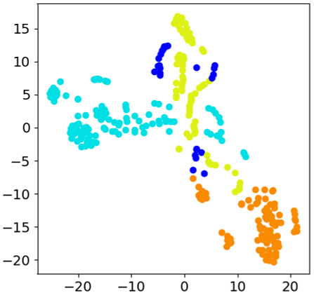
(a) Visible (Base)

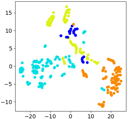
(b) Auxiliary (Base)

(c) Visible (Ours)

(d) Auxiliary (Ours)

Figure 8: TSNE visualization [48] for final encoder features from Base (w/o SMMCL) and Ours (w SMMCL) on a low-light scene in LLRGBD-synthetic. Each color corresponds to a semantic class.

	Model1	Model2	Model3	Model4
Cross-Modal	✗	✓	✗	✓
Intra-Modal	✗	✗	✓	✓
mIoU (%)	66.02	68.62	68.52	68.76

Table 5: Effectiveness study of our supervised multi-modal contrastive learning approach on low-light indoor scenes.

4.5 Ablation Study

We thoroughly analyze our supervised multi-modal contrastive learning approach in this section. Other ablations are provided in the supplementary material.

Basic Ablations. Table 5 studies the effectiveness of our approach on low-light indoor scenes. In a comparison of Model₁, i.e., Base (w/o SMMCL), which is trained with only a cross-entropy loss, and Model₂, which is trained by adding the cross-modal contrastive loss, Model₂ yields a $2.6\%$ improvement and accuracy of $68.62\%$. By adding the intra-modal contrastive losses, Model₃ produces accuracy of $68.52\%$. Further, by jointly introducing cross-modal and intra-modal contrast, Model₄, i.e., Ours (w SMMCL), achieves the best accuracy, $68.76\%$.

TSNE Visualization. Figure 8 visualizes the final encoder features, i.e., $\textbf{F}_{vis}^{4}$ and $\textbf{F}_{aux}^{4}$, learned by Base (w/o SMMCL) and Ours (w SMMCL). As shown in subfigures (a-b), features learned by Base (w/o SMMCL) show low semantic discriminability, with points from different classes being in a mixed distribution. By contrast, in features learned by Ours (w SMMCL), i.e., subfigures (c-d), points belonging to the same class are closer and form clearer clusters. This demonstrates that our approach effectively encourages the feature spaces learned from multi-modal images with limited semantics to show higher semantic discriminability.

Visual Comparisons of Base and Ours. As a more intuitive validation, we compare Base (w/o SMMCL) and Ours (w SMMCL) in Fig. 9. Thanks to our multi-modal contrastive learning approach, our model can predict different semantic classes more accurately and understand dark scenes from multi-modal images more effectively.

Comparisons with Other Approaches. Since our approach is the first supervised multi-modal contrastive learning approach for image segmentation, we comprehensively compare it with an unsupervised multi-modal approach [36] and a supervised single-modal approach [26]. Unlike these methods which need to generate samples via augmentation or consider only single-modal region features, we leverage class labels to effectively align pixel embeddings across different modalities. Table 6 shows that our approach significantly outperforms them on various tasks. This demonstrates again our effectiveness, and justifies the superiority of our supervised paradigm and the benefit of fully considering the cross-modal context-geometry correspondence.

Broader Significance. In our tasks, the adoption of our approach can help overcome a learning bias problem caused by “invalid” auxiliary modality. We provide additional discussions in the supplementary material.

(a) Visible

(b) Auxiliary

(c) GT

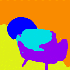
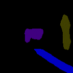
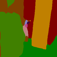
(d) Base

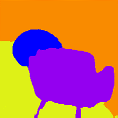
(e) Ours

Figure 9: Visual comparisons of Base (w/o SMMCL) and Ours (w SMMCL) on low-light, nighttime, and normal-light scenes.

Method	S	MM	Low	Night	Normal
			mIoU (%)
Base	-	-	66.02	58.44	54.70
Base + [36]	✗	✓	66.54	58.93	55.10
Base + [26]	✓	✗	68.02	59.48	55.46
Base + SMMCL	✓	✓	68.76	60.00	55.77

Table 6: Comparisons with other contrastive learning approaches. Base is the baseline, Base (w/o SMMCL). S denotes supervised. MM denotes multi-modal.

5 Conclusions

We tackle dark scene understanding by contrasting visible and auxiliary images with limited semantic information. We propose a supervised multi-modal contrastive learning approach to boost the learning on the two modalities and encourage them to be semantic-discriminative in the feature space. We demonstrate the effectiveness, generalizability, and applicability of our approach on low-light indoor scenes, nighttime outdoor scenes, normal-light scenes, and different image modalities. We believe our work will contribute to dark scene semantic segmentation, which is a challenging but important task in life, and can inspire further progress in multi-modal scene understanding.

Acknowledgements. This work was supported by the RIKEN Junior Research Associate (JRA) Program and JST, FOREST under Grant Number JPMJFR206S.

References

- [1] Mohamed Afham, Isuru Dissanayake, Dinithi Dissanayake, Amaya Dharmasiri, Kanchana Thilakarathna, and Ranga Rodrigo. CrossPoint: Self-supervised cross-modal contrastive learning for 3d point cloud understanding. In CVPR, 2022.
- [2] Iñigo Alonso, Alberto Sabater, David Ferstl, Luis Montesano, and Ana C. Murillo. Semi-supervised semantic segmentation with pixel-level contrastive learning from a class-wise memory bank. In ICCV, 2021.
- [3] Gedas Bertasius, Jianbo Shi, and Lorenzo Torresani. Semantic segmentation with boundary neural fields. In CVPR, 2016.
- [4] Jinming Cao, Hanchao Leng, Dani Lischinski, Danny Cohen-Or, Changhe Tu, and Yangyan Li. ShapeConv: Shape-aware convolutional layer for indoor RGB-D semantic segmentation. In ICCV, 2021.
- [5] Liang-Chieh Chen, George Papandreou, IIasonas Kokkinos, Kevin Murphy, and Allan Yuille. DeepLab: semantic image segmentation with deep convolutional nets, atrous convolution, and fully connected CRFs. IEEE TPAMI, 2017.
- [6] Liang-Chieh Chen, George Papandreou, Florian Schroff, and Hartwig Adam. Rethinking atrous convolution for semantic image segmentation. arXiv preprint arXiv:1706.05587, 2017.
- [7] Liang-Chieh Chen, Yukun Zhu, George Papandreou, Florian Schroff, and Hartwig Adam. Encoder-decoder with atrous separable convolution for semantic image segmentation. In ECCV, 2018.
- [8] Lin-Zhuo Chen, Zheng Lin, Ziqin Wang, Yong-Liang Yang, and Ming-Ming Cheng. Spatial information guided convolution for real-time RGBD semantic segmentation. IEEE TIP, 2021.
- [9] Ting Chen, Simon Kornblith, Mohammad Norouzi, and Geoffrey Hinton. A simple framework for contrastive learning of visual representations. arXiv preprint arXiv:2002.05709, 2020.
- [10] Xiaokang Chen, Kwan-Yee Lin, Jingbo Wang, Wayne Wu, Chen Qian, Hongsheng Li, and Gang Zeng. Bi-directional cross-modality feature propagation with separation-and-aggregation gate for RGB-D semantic segmentation. In ECCV, 2020.
- [11] Zhe Chen, Yuchen Duan, Wenhai Wang, Junjun He, Tong Lu, Jifeng Dai, and Yu Qiao. Vision transformer adapter for dense predictions. In ICLR, 2023.
- [12] Ziteng Cui, Lin Gu, Xiao Sun, Yu Qiao, and Tatsuya Harada. Aleth-NeRF: Low-light condition view synthesis with concealing fields. arXiv preprint arXiv:2303.05807, 2023.
- [13] Ziteng Cui, Guo-Jun Qi, Lin Gu, Shaodi You, Zenghui Zhang, and Tatsuya Harada. Multitask AET with orthogonal tangent regularity for dark object detection. In ICCV, 2021.
- [14] Dengxin Dai and Luc Van Gool. Dark model adaptation: Semantic image segmentation from daytime to nighttime. In ITSC, 2018.
- [15] Xueqing Deng, Peng Wang, Xiaochen Lian, and Shawn Newsam. NightLab: A dual-level architecture with hardness detection for segmentation at night. In CVPR, 2022.
- [16] Henghui Ding, Xudong Jiang, Ai Qun Liu, Nadia Magnenat Thalmann, and Gang Wang. Boundary-aware feature propagation for scene segmentation. In ICCV, 2019.
- [17] Jun Fu, Jing Liu, Haijie Tian, Yong Li, Yongjun Bao, Zhiwei Fang, and Hanqing Lu. Dual attention network for scene segmentation. In CVPR, 2019.
- [18] Angus Fung, Beno Benhabib, and Goldie Nejat. Robots autonomously detecting people: A multimodal deep contrastive learning method robust to intraclass variations. IEEE Robotics and Automation Letters, 2023.
- [19] Huan Gao, Jichang Guo, Guoli Wang, and Qian Zhang. Cross-domain correlation distillation for unsupervised domain adaptation in nighttime semantic segmentation. In CVPR, 2022.
- [20] Rui Gong, Qin Wang, Martin Danelljan, Dengxin Dai, and Luc Van Gool. Continuous pseudo-label rectified domain adaptive semantic segmentation with implicit neural representations. In CVPR, 2023.
- [21] Meng-Hao Guo, Cheng-Ze Lu, Qibin Hou, Zhengning Liu, Ming-Ming Cheng, and Shi-Min Hu. SegNeXt: Rethinking convolutional attention design for semantic segmentation. In NeurIPS, 2022.
- [22] Saurabh Gupta, Ross Girshick, Pablo Arbelaez, and Jitendra Malik. Learning rich features from RGB-D images for object detection and segmentation. In ECCV, 2014.
- [23] Qishen Ha, Kohei Watanabe, Takumi Karasawa, Yoshitaka Ushiku, and Tatsuya Harada. MFNet: Towards real-time semantic segmentation for autonomous vehicles with multi-spectral scenes. In IROS, 2017.
- [24] Raia Hadsell, Sumit Chopra, and Yann LeCun. Dimensionality reduction by learning an invariant mapping. In CVPR, 2006.
- [25] Kaiming He, Haoqi Fan, Yuxin Wu, Saining Xie, and Ross Girshick. Momentum contrast for unsupervised visual representation learning. In CVPR, 2020.
- [26] Hanzhe Hu, Jinshi Cui, and Liwei Wang. Region-aware contrastive learning for semantic segmentation. In ICCV, 2021.
- [27] Zilong Huang, Xinggang Wang, Yunchao Wei, Lichao Huang, Humphrey Shi, Wenyu Liu, and Thomas S. Huang. CCNet: Criss-cross attention for semantic segmentation. IEEE TPAMI, 2020.
- [28] Maximilian Jaritz, Tuan-Hung Vu, Raoul de Charette, Emilie Wirbel, and Patrick Pérez. Cross-modal learning for domain adaptation in 3D semantic segmentation. In TPAMI, 2022.
- [29] Prannay Khosla, Piotr Teterwak, Chen Wang, Aaron Sarna, Yonglong Tian, Phillip Isola, Aaron Maschinot, Ce Liu, and Dilip Krishnan. Supervised contrastive learning. In NeurIPS, 2020.
- [30] Youngwan Lee, Jonghee Kim, Jeffrey Willette, and Sung Ju Hwang. MPViT: Multi-path vision transformer for dense prediction. In CVPR, 2022.
- [31] Gongyang Li, Yike Wang, Zhi Liu, Xinpeng Zhang, and Dan Zeng. RGB-T semantic segmentation with location, activation, and sharpening. IEEE TCSVT, 2022.
- [32] Wenyu Liu, Wentong Li, Jianke Zhu, Miaomiao Cui, Xuansong Xie, and Lei Zhang. Improving nighttime driving-scene segmentation via dual image-adaptive learnable filters. arXiv preprint arXiv:2207.01331, 2022.
- [33] Yunze Liu, Qingnan Fan, Shanghang Zhang, Hao Dong, Thomas Funkhouser, and Li Yi. Contrastive multimodal fusion with TupleInfoNCE. In ICCV, 2021.
- [34] Jonathan Long, Evan Shelhamer, and Trevor Darrell. Fully convolutional networks for semantic segmentation. In CVPR, 2015.
- [35] Ilya Loshchilov and Frank Hutter. Decoupled weight decay regularization. In ICLR, 2019.
- [36] Johannes Meyer, Andreas Eitel, Thomas Brox, and Wolfram Burgard. Improving unimodal object recognition with multimodal contrastive learning. In IROS, 2020.
- [37] Duo Peng, Yinjie Lei, Wen Li, Pingping Zhang, and Yulan Guo. Sparse-to-dense feature matching: Intra and inter domain cross-modal learning in domain adaptation for 3D semantic segmentation. In ICCV, 2021.
- [38] Theodoros Pissas, Claudio S. Ravasio, Lyndon Da Cruz, and Christos Bergeles. Multi-scale and cross-scale contrastive learning for semantic segmentation. In ECCV, 2022.
- [39] Christos Sakaridis, Dengxin Dai, and Luc Van Gool. Guided curriculum model adaptation and uncertainty-aware evaluation for semantic nighttime image segmentation. In ICCV, 2019.
- [40] Christos Sakaridis, Dengxin Dai, and Luc Van Gool. Map-guided curriculum domain adaptation and uncertainty-aware evaluation for semantic nighttime image segmentation. IEEE TPAMI, 2020.
- [41] Nathan Silberman, Derek Hoiem, Pushmeet Kohli, and Rob Fergus. Indoor segmentation and support inference from RGBD images. In ECCV, 2012.
- [42] Robin Strudel, Ricardo Garcia, Ivan Laptev, and Cordelia Schmid. Segmenter: Transformer for semantic segmentation. In ICCV, 2021.
- [43] Ke Sun, Bin Xiao, Dong Liu, and Jingdong Wang. Deep high-resolution representation learning for human pose estimation. In CVPR, 2019.
- [44] Tao Sun, Mattia Segu, Janis Postels, Yuxuan Wang, Luc Van Gool, Bernt Schiele, Federico Tombari, and Fisher Yu. SHIFT: a synthetic driving dataset for continuous multi-task domain adaptation. In CVPR, 2022.
- [45] Yuxiang Sun, Weixun Zuo, and Ming Liu. RTFNet: RGB-thermal fusion network for semantic segmentation of urban scenes. IEEE Robot. Autom. Lett., 2019.
- [46] Xin Tan, Ke Xu, Ying Cao, Yiheng Zhang, Lizhuang Ma, and Rynson W. H. Lau. Night-time scene parsing with a large real dataset. IEEE TIP, 2021.
- [47] Aaron van den Oord, Yazhe Li, and Oriol Vinyals. Representation learning with contrastive predictive coding. arXiv preprint arXiv:1807.03748, 2018.
- [48] Laurens van der Maaten and Geoffrey Hinton. Visualizing data using t-SNE. Journal of machine learning research, 2008.
- [49] Johan Vertens, Jannik Zürn, and Wolfram Burgard. HeatNet: Bridging the day-night domain gap in semantic segmentation with thermal images. In IROS, 2020.
- [50] Jingdong Wang, Ke Sun, Tianheng Cheng, Borui Jiang, Chaorui Deng, Yang Zhao, Dong Liu, Yadong Mu, Mingkui Tan, Xinggang Wang, Wenyu Liu, and Bin Xiao. Deep high-resolution representation learning for visual recognition. IEEE TPAMI, 2020.
- [51] Weiyue Wang and Ulrich Neumann. Depth-aware cnn for RGB-D segmentation. In ECCV, 2018.
- [52] Wenguan Wang, Tianfei Zhou, Fisher Yu, Jifeng Dai, Ender Konukoglu, and Luc Van Gool. Exploring cross-image pixel contrast for semantic segmentation. In ICCV, 2021.
- [53] Yikai Wang, Xinghao Chen, Lele Cao, Wenbing Huang, Fuchun Sun, and Yunhe Wang. Multimodal token fusion for vision transformers. In CVPR, 2022.
- [54] Yikai Wang, Wenbing Huang, Fuchun Sun, Tingyang Xu, Yu Rong, and Junzhou Huang. Deep multimodal fusion by channel exchanging. In NeurIPS, 2020.
- [55] Yikai Wang, Fuchun Sun, Wenbing Huang, Fengxiang He, and Dacheng Tao. Channel exchanging networks for multimodal and multitask dense image prediction. IEEE TPAMI, 2022.
- [56] Xinyi Wu, Zhenyao Wu, Hao Guo, Lili Ju, and Song Wang. DANNet: A one-stage domain adaptation network for unsupervised nighttime semantic segmentation. In CVPR, 2021.
- [57] Zhirong Wu, Yuanjun Xiong, X Yu Stella, and Dahua Lin. Unsupervised feature learning via non-parametric instance discrimination. In CVPR, 2018.
- [58] Enze Xie, Wenhai Wang, Zhiding Yu, Anima Anandkumar, Jose M Alvarez, and Ping Luo. SegFormer: Simple and efficient design for semantic segmentation with transformers. In NeurIPS, 2021.
- [59] Zhifeng Xie, Sen Wang, Ke Xu, Zhizhong Zhang, Xin Tan, Yuan Xie, and Lizhuang Ma. Boosting night-time scene parsing with learnable frequency. arXiv preprint arXiv:2208.14241, 2022.
- [60] Yajie Xing, Jingbo Wang, and Gang Zeng. Malleable 2.5D convolution: Learning receptive fields along the depth-axis for RGB-D scene parsing. In ECCV, 2020.
- [61] Xiaowen Ying and Mooi Choo Chuah. UCTNet: Uncertainty-aware cross-modal transformer network for indoor rgb-d semantic segmentation. In ECCV, 2022.
- [62] Changqian Yu, Jingbo Wang, Changxin Gao, Gang Yu, Chunhua Shen, and Nong Sang. Context prior for scene segmentation. In CVPR, 2020.
- [63] Yuhui Yuan, Rao Fu, Lang Huang, Weihong Lin, Chao Zhang, Xilin Chen, and Jingdong Wang. HRFormer: High-resolution transformer for dense prediction. In NeurIPS, 2021.
- [64] Hang Zhang, Kristin Dana, Jianping Shi, Zhongyue Zhang, Xiaogang Wang, Ambrish Tyagi, and Amit Agrawal. Context encoding for semantic segmentation. In CVPR, 2018.
- [65] Han Zhang, Jing Yu Koh, Jason Baldridge, Honglak Lee, and Yinfei Yang. Cross-modal contrastive learning for text-to-image generation. In CVPR, 2021.
- [66] Jiaming Zhang, Huayao Liu, Kailun Yang, Xinxin Hu, Ruiping Liu, and Rainer Stiefelhagen. CMX: Cross-modal fusion for RGB-X semantic segmentation with transformers. IEEE Transactions on Intelligent Transportation Systems, 2023.
- [67] Ning Zhang, Francesco Nex, Norman Kerle, and George Vosselman. Towards learning low-light indoor semantic segmentation with illumination-invariant features. The International Archives of Photogrammetry, Remote Sensing and Spatial Information Sciences, 2021.
- [68] Ning Zhang, Francesco Nex, Norman Kerle, and George Vosselman. LISU: Low-light indoor scene understanding with joint learning of reflectance restoration. ISPRS J. Photogramm. Remote Sens., 2022.
- [69] Qiang Zhang, Shenlu Zhao, Yongjiang Luo, Dingwen Zhang, Nianchang Huang, and Jungong Han. ABMDRNet: Adaptive-weighted bi-directional modality difference reduction network for RGB-T semantic segmentation. In CVPR, 2021.
- [70] Hengshuang Zhao, Jianping Shi, Xiaojuan Qi, Xiaogang Wang, and Jiaya Jia. Pyramid scene parsing network. In CVPR, 2017.
- [71] Hengshuang Zhao, Yi Zhang, Shu Liu, Jianping Shi, Chen Change Loy, Dahua Lin, and Jiaya Jia. PSANet: Point-wise spatial attention network for scene parsing. In ECCV, 2018.
- [72] Xiangyun Zhao, Raviteja Vemulapalli, Philip Andrew Mansfield, Boqing Gong, Bradley Green, Lior Shapira, and Ying Wu. Contrastive learning for label efficient semantic segmentation. In ICCV, 2021.
- [73] Mingmin Zhen, Jinglu Wang, Lei Zhou, Shiwei Li, Tianwei Shen, Jiaxiang Shang, Tian Fang, and Long Quan. Joint semantic segmentation and boundary detection using iterative pyramid contexts. In CVPR, 2020.
- [74] Zilong Zhong, Zhong Qiu Lin, Rene Bidart, Xiaodan Hu, Ibrahim Ben Daya, Zhifeng Li, Wei-Shi Zheng, Jonathan Li, and Alexander Wong. Squeeze-and-attention networks for semantic segmentation. In CVPR, 2020.
- [75] Wujie Zhou, Shaohua Dong, Caie Xu, and Yaguan Qian. Edge-aware guidance fusion network for RGB–thermal sceneparsing. In AAAI, 2022.
- [76] Wujie Zhou, Jinfu Liu, Jingsheng Lei, Lu Yu, and Jenq-Neng Hwang. GMNet: Graded-feature multilabel-learning network for RGB-thermal urban scene semantic segmentation. IEEE TIP, 2021.
- [77] Yizhou Zhou, Xiaoyan Sun, Zheng-Jun Zha, and Wenjun Zeng. Context-reinforced semantic segmentation. In CVPR, 2019.
- [78] Mohammadreza Zolfaghari, Yi Zhu, Peter Gehler, and Thomas Brox. CrossCLR: Cross-modal contrastive learning for multi-modal video representations. In ICCV, 2021.