New algorithm of measuring gravitational wave radiation from rotating binary system

Abstract

In order to investigate the gravitational wave (GW) radiation, without appealing to the tensorial formalism of the linearized general relativity, we formulate the so-called modified linearized general relativity (MLGR). As an application of the MLGR, we construct a novel paradigm of measuring the GW radiation from a binary system of compact objects, to theoretically interpret their phenomenology. To do this, we formulate the mass scalar and mass vector potentials for the merging binary compact objects, from which we construct the mass magnetic field in addition to the mass electric one which also includes the mass vector potential effect. Next, defining the mass Poyinting vector in terms of the mass electric and mass magnetic fields, we construct the GW radiation intensity profile possessing a prolate ellipsoid geometry due to the merging binary compact objects source. At a given radial distance from the binary compact objects, the GW radiation intensity on the revolution axis of the binary compact objects is shown to be twice that on the equatorial plane. Moreover, we explicitly obtain the total radiation power of the GW, which has the same characteristic as that of the electromagnetic wave in the rotating charge electric dipole moment. We also find that, in no distorting limit of the merging binary compact objects, the compact objects do not yield the total GW radiation power, consistent with the result of the linearized general relativity.

I Introduction

Exploiting the tensorial formalism for the gravity, the linearized general relativity (LGR) wald84 ; hobson06 has been investigated to describe the gravitational wave (GW) radiation from a binary system of compact objects (namely stars or black holes) for instance. To be specific, in order to study the physical phenomenology in the LGR, we need to assume that the gravity fields are weak so that the gravitational field equations can be linearized. Next it is well known that, in vacuum of the LGR, the binary compact objects oscillating in time emit spin-two gravitons which are quanta of the GW. Mathematically the spin-two gravitons originate from the second rank tensor associated with the curved spacetime metric $g_{\alpha\beta}$ pauli39 ; wald84 . In order to construct the GW which is transverse to the GW propagating direction and yields the spin-two graviton, we have exploited the ad hoc transverse-traceless gauge wald84 ; hobson06 . In contrast, the spin-one photons which are quanta of the electromagnetic (EM) wave in vacuum are delineated in terms of the vectorial quantities of the charge scalar and charge vector potentials defined on the flat spacetime.

On the other hand, since the first GW was detected by Advanced LIGO aasi15 , there have been lots of progresses in an observational astrophysics. In particular, the third generation network of ground-based detectors reitze19 is currently proposed to obtain improved sensitivities, compared to those of the Advanced LIGO detector. Recently, in order to constrain cosmology, a theoretical probe of cosmology which exploits population level properties of lensed GW detections has been proposed  jana23 . Next, since the gamma ray burst (GRB) discovery was published strong73 , to elucidate the GRB associated with the magnetar (namely highly-magnetized neutron star) for instance hurley21 , we have observed many theoretical models including the Dirac type relativistic massive photon model hong22 , where the anti-photon corresponding to the negative energy solution is proposed as a candidate for an intense radiation flare of the GRB. Next, the first neutron star binary PSR B1913+16 has been discovered showing that its orbit was losing energy due to the emission of the GW hulse75 . The GW detector network has observed the GW merger event originating from binary neutron star GW170817 in 2017 abbott2017a ; grb1 ; goldstein2017 . Note that the GW170817 merger event has been known to be consistent with the GRB of GRB170817A grb1 ; goldstein2017 . To be specific, the GW is supposed to be produced from neutron star oscillations related with magnetar giant flares and the corresponding GRB kaspi2017 ; ligo2023 .

In this paper, we will propose a new theoretical paradigm of the modified linearized general relativity (MLGR), in which we will formulate the Green retarded wald84 ; hobson06 mass scalar and mass vector potentials of a binary system of compact objects. Using these potentials in the MLGR, we will next construct the mass electric and mass magnetic fields. In particular, in order to formulate the non-vanishing mass magnetic field, we will introduce the distortion of the spirally merging binary compact objects during one cycle of their revolution. Making use of the mass electric and mass magnetic fields, we will find the mass Poyinting vector which is exploited to construct a theoretical scheme of measuring the GW radiation from a binary system of compact objects. Moreover, introducing the traceless transverse gauge, we will study the GW of the binary compact objects in the LGR.

In Sec. 2 we will formulate the MLGR. In Sec. 3, as an application of the MLGR, we will investigate the phenomenology of the merging binary compact objects. To do this, we will explicitly formulate the physical quantities such as the mass scalar and mass vector potentials, and the mass Poyinting vector. We will also study the traceless transverse gauge in the LGR. Sec. 4 includes conclusions. In Appendix A, we will pedagogically study the EM radiation from the rotating charge electric dipole moment.

II Set up of MLGR algorithm

In this section, we will formulate the MLGR which includes explicitly the mass current degrees of freedom (DOF). To do this, in the linearized general relativity wald84 ; hobson06 , we first assume that the deviation $h_{\alpha\beta}$ of the spacetime metric $g_{\alpha\beta}$ from a flat metric $\eta_{\alpha\beta}$ is small: $g_{\alpha\beta}=\eta_{\alpha\beta}+h_{\alpha\beta}$. After some algebra we can find the linearized Einstein equation wald84

$$-\frac{1}{2}\square\bar{h}_{\alpha\beta}+\partial^{\gamma}\partial_{(\alpha}\bar{h}_{\beta)\gamma}-\frac{1}{2}\eta_{\alpha\beta}\partial^{\gamma}\partial^{\delta}\bar{h}_{\gamma\delta}=\frac{8\pi G}{c^{4}}T_{\alpha\beta},$$ (2.1)

where $\square=\partial^{\beta}\partial_{\beta}$ with the metric $(-1,+1,+1,+1)$ and $T_{\alpha\beta}$ is the stress-energy tensor. Here the trace reversed perturbation $\bar{h}_{\alpha\beta}$ is given by $\bar{h}_{\alpha\beta}=h_{\alpha\beta}-\frac{1}{2}\eta_{\alpha\beta}h$ and $h=\eta^{\alpha\beta}h_{\alpha\beta}$. Next exploiting (2.1) and the Lorentz gauge condition (LGC) in the gravity

$$\partial^{\beta}\bar{h}_{\alpha\beta}=0,$$ (2.2)

we arrive at

$$\square\bar{h}_{\alpha\beta}=-\frac{16\pi G}{c^{4}}T_{\alpha\beta}.$$ (2.3)

Now we consider the MLGR where we have the non-vanishing $\bar{h}^{00}$ and $\bar{h}^{0i}$ $(i=1,2,3)$, together with

$$\bar{h}^{ij}=0.$$ (2.4)

We define in the MLGR the time-time component of the trace reversed perturbation $\bar{h}^{00}$ and the corresponding stress energy tensor $T^{00}$ as

$$\bar{h}^{00}=-\frac{4}{c}A_{M}^{0},~{}~{}~{}T^{00}=c^{2}\rho_{M},$$ (2.5)

where $\rho_{M}$ is the mass density. Here the subscript $M$ denotes the mass related quantities and will be applied to the gravitational interaction physical quantities from now on. Inserting (2.5) into (2.3) yields

$$\square A_{M}^{0}=\frac{4\pi G}{c}\rho_{M},$$ (2.6)

implying that we have the dynamical DOF in the MLGR. Note that, in the static case, (2.6) and $\phi_{M}\equiv cA_{M}^{0}$ yields $\nabla^{2}\phi_{M}=4\pi G\rho_{M}$ which is consistent with the Newtonian gravity goldstein80 ; marion04 ; wald84 .

Next in the MLGR we define the time-space components of the trace reversed perturbation $\bar{h}^{0i}$ and the stress energy tensor $T^{0i}$ as

$$\bar{h}^{0i}=-\frac{4}{c}A^{i}_{M},~{}~{}~{}T^{0i}=cJ^{i}_{M},$$ (2.7)

where $J^{i}_{M}\equiv\rho_{M}v^{i}$ is the mass current density associated with the mass current velocity $v^{i}$. In the MLGR, inserting (2.7) into (2.3) produces

$$\square A^{i}_{M}=\frac{4\pi G}{c^{2}}J^{i}_{M}.$$ (2.8)

Combining (2.6) and (2.8), we find the covariant form of the equations of motion

$$\square A^{\alpha}_{M}=\frac{4\pi G}{c^{2}}J^{\alpha}_{M},$$ (2.9)

where $A_{M}^{\alpha}=\left(\frac{\phi_{M}}{c},A_{M}^{i}\right)$ and the four mass current density is defined by $J^{\alpha}_{M}=(c\rho_{M},J^{i}_{M})$. Note that the LGC in (2.2) is rewritten as

$$\partial_{\alpha}A^{\alpha}_{M}=0.$$ (2.10)

Exploiting $A^{\alpha}_{M}$ in (2.5) and (2.7), we can find

$$A^{\alpha}_{M}=-\frac{c}{4}\bar{h}^{0\alpha},$$ (2.11)

to yield the equation of motion

$$\square\bar{h}^{0\alpha}=-\frac{16\pi G}{c^{3}}J^{\alpha}_{M}.$$ (2.12)

Note that the LGC in (2.10) becomes

$$\partial_{\alpha}\bar{h}^{0\alpha}=0.$$ (2.13)

Now we investigate the GW defined in the vacuum. To do this, inserting $J^{\alpha}_{M}=0$ into (2.12) and exploiting $\bar{h}^{0\alpha}$ in (2.11), we obtain the wave equation for the non-vanishing field $\bar{h}^{0\alpha}$ (or $A_{M}^{\alpha}$)

$$\square\bar{h}^{0\alpha}=\square A_{M}^{\alpha}=0.$$ (2.14)

Note that the wave equations in (2.14) in the MLGR describe a massless spin-one graviton propagating in the flat spacetime, similar to a massless spin-one photon propagating in the flat spacetime. To be specific, (2.14) explains the graviton of gravitational field.

Next it seems appropriate to comment on the spin of the graviton in the MLGR. In vacuum with $T_{\alpha\beta}=0$ in (2.3), we end up with the wave equation $\square\bar{h}_{\alpha\beta}=0$ which could describe a massless spin-two graviton propagating in the flat spacetime pauli39 ; wald84 . However, if we consider only the physically meaningful wave equation for $A^{\alpha}_{M}$ in (2.14) obtained from that for $\bar{h}^{0\alpha}$ $(\alpha=0,1,2,3)$, we mathematically find a massless spin-one graviton whose properties are well defined in the MLGR. Note that the condition $\bar{h}^{ij}=0$ in (2.4) reduces the number of independent components of $\bar{h}^{\alpha\beta}$ to four. The independent components $(\bar{h}^{00},\bar{h}^{0i})$ thus correspond to the four components of $A^{\alpha}_{M}$. Next we explicitly find the solution of the GW field equation in (2.14) as follows

$$\bar{h}^{0\alpha}=\epsilon^{\alpha}e^{ik_{\mu}x^{\mu}},$$ (2.15)

where $k^{\mu}$ is the GW four-vector. Here $\epsilon^{\alpha}$ is the constant amplitude vector corresponding to the GW polarizations. Inserting (2.15) into (2.14), we find $k_{\alpha}k^{\alpha}=0$ to yield

$$k^{\alpha}=(k,0,0,k),$$ (2.16)

which describes the massless spin-one graviton. Making use of (2.15) and the LGC in (2.13), we obtain

$$k_{\alpha}\epsilon^{\alpha}=0,$$ (2.17)

to produce $\epsilon^{0}=\epsilon^{3}$.

Now we exploit the fact that the LGC in (2.13) is preserved by the gauge transformation $\bar{h}^{0\alpha}\rightarrow\bar{h}^{0\alpha}+\partial^{\alpha}\psi$ if $\square\psi=0$ wald84 ; hobson06 . We assume $\psi=\epsilon e^{ik_{\mu}x^{\mu}}$ and $\bar{h}^{\prime 0\alpha}=\epsilon^{\prime\alpha}e^{ik_{\mu}x^{\mu}}$, and then we exploit the gauge transformation equation $\bar{h}^{\prime 0\alpha}=\bar{h}^{0\alpha}+\partial^{\alpha}\psi$ to yield

$$\epsilon^{\prime\alpha}=\epsilon^{\alpha}+i\epsilon k^{\alpha}.$$ (2.18)

Using (2.16) and (2.18), we explicitly find the non-trivial relation $\epsilon^{\prime 0}=\epsilon^{0}+i\epsilon k$. Next, exploiting the ansatz $\epsilon=\frac{i}{k}\epsilon^{0}$, we find $\epsilon^{\prime 0}=0$. Dropping the primes in $\epsilon^{\prime\alpha}$ we obtain

$$\epsilon^{\alpha}=(0,\epsilon^{1},\epsilon^{2},0),$$ (2.19)

implying that the GW is transverse to the propagation direction $k^{\alpha}$ in (2.16). Note that $\epsilon^{\alpha}$ in (2.19) thus satisfies the identity $k_{\alpha}\epsilon^{\alpha}=0$ in (2.17) as expected.

Next we have several comments on the GW phenomenology in terms of $\epsilon^{\alpha}$ in (2.19). First, in the cases of $\epsilon^{\alpha}=(0,\epsilon^{1},0,0)$ and $\epsilon^{\alpha}=(0,0,\epsilon^{2},0)$, as the GW passes a free positive test charge, the test charge will oscillate in the $x$ and $y$ directions with a magnitude changing sinusoidally with time, respectively, following the GW wave relation in (2.15). Second, in the cases of $\epsilon^{\alpha}=(0,\epsilon^{1},i\epsilon^{1},0)$ and $\epsilon^{\alpha}=(0,\epsilon^{1},-i\epsilon^{1},0)$, the GW polarizations yield left-circularly and right-circularly polarized GWs, and then the test charge will move in the corresponding circles, respectively. Third, in the general cases of $\epsilon^{\alpha}=(0,\epsilon^{1},i\bar{\epsilon}^{1},0)$ and $\epsilon^{\alpha}=(0,\epsilon^{1},-i\bar{\epsilon}^{1},0)$ $(\epsilon^{1}\neq\bar{\epsilon}^{1})$, the GW polarizations produce left-elliptic and right-elliptic polarized GWs, respectively, and thus the test charge will move in the corresponding ellipses.

Now we investigate the properties of the massive graviton parenthetically. As in the case of the massive photon hong22 , we find the identity $k_{\alpha}\epsilon^{\alpha}\neq 0$ for the massive graviton, since for the massive graviton we have longitudinal component in addition to transverse ones, similar to the phonon associated with massive particle lattice vibrations phonon . Note that $\epsilon^{\alpha}$ is a polarization vector possessing the spacetime index $\alpha$ $(\alpha=0,1,2,3)$ which is the same as the massive graviton spin index and is needed to incorporate minimally the spin DOF for the massive graviton. Note also that, as in the case of the GRB in the Dirac type relativistic massive photon model hong22 , the massive graviton could be interpreted as a spin-one GRB-like particle grb1 ; goldstein2017 . The GRB-like graviton corresponding to its negative energy solution could then be regarded as an anti-graviton, which could be a candidate for an intense radiation flare of the GRB of GRB170817A grb1 ; goldstein2017 associated with the binary compact objects merger event GW170817. Note that the massive anti-graviton could be described in terms of the massive gauge boson possessing a finite radius as in the massive photon in the stringy photon model hong211 .

III Gravitational wave radiation from merging binary compact objects

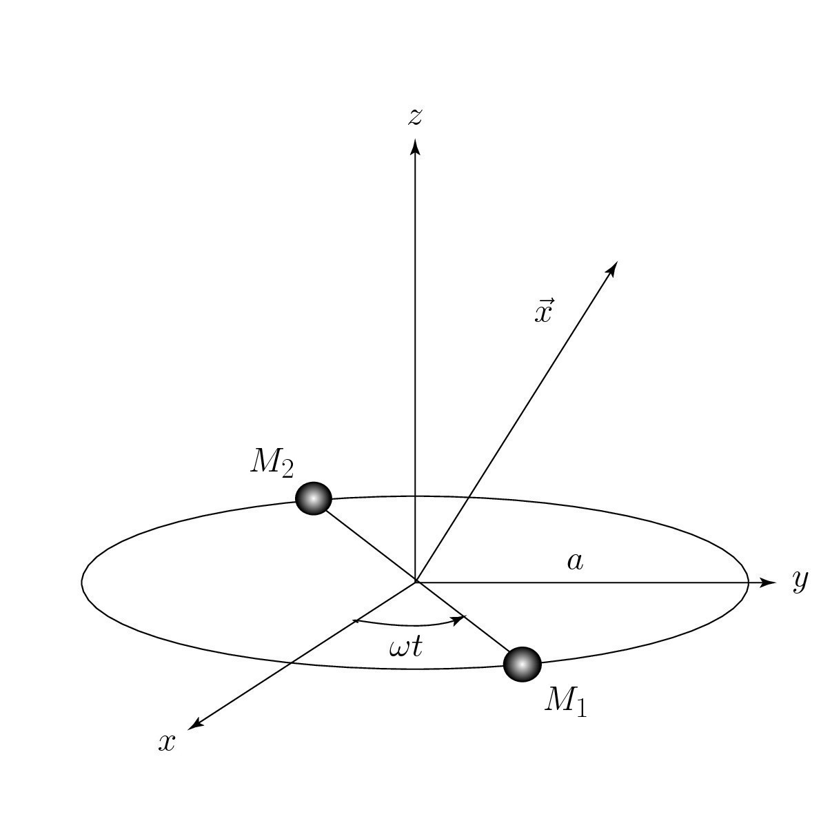
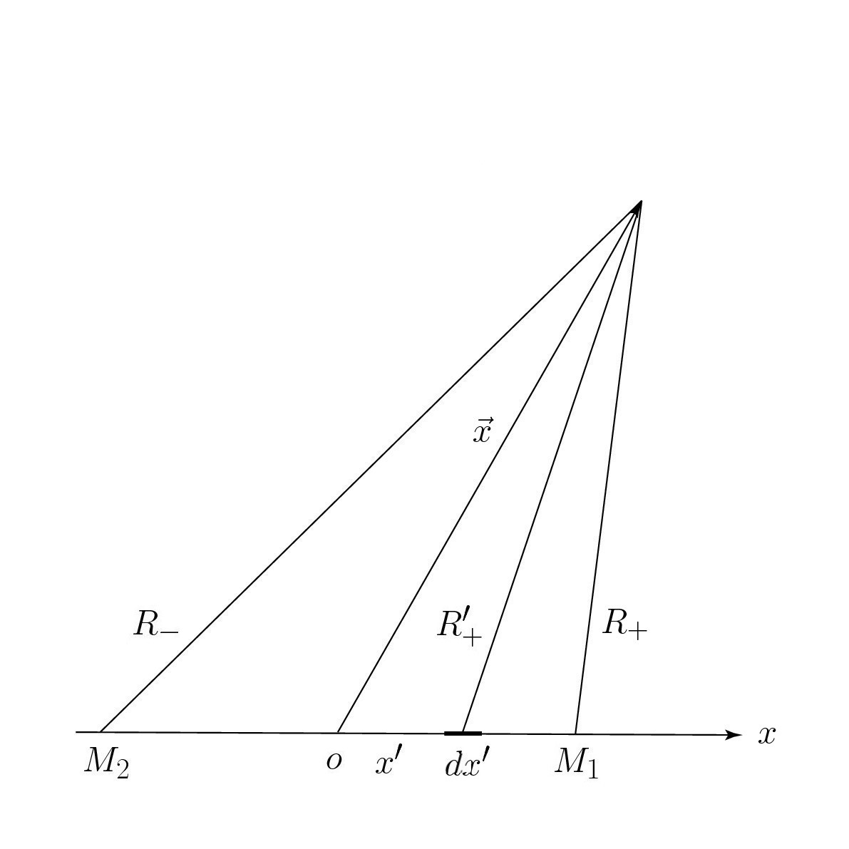
Figure 1: (a) The schematic diagram for a binary system of compact objects $M_{1}$ and $M_{2}$ of equal mass $M$ which co-rotate in circular orbits of radius $a$ about their common center of mass located at the origin, with an angular frequency $\omega$. (b) The diagram for the geometry of $R_{\pm}$ for the retarded mass scalar potentials $\phi_{M}^{I}$ in (3.21) and $R_{+}^{\prime}$ for the retarded mass vector potentials $\vec{A}_{M}^{I}$ in (3.25). Here $\vec{x}=r(\hat{x}\sin\theta\cos\phi+\hat{y}\sin\theta\sin\phi+\hat{z}\cos\theta)$ denotes a radial vector from the origin $o$ to an observation point.

In this section, in the MLGR we investigate a binary system of merging compact objects which possesses masses $M_{1}$ and $M_{2}$ rotating on the $x$-$y$ plane. We assume that for simplicity the two compact objects $M_{1}$ and $M_{2}$ of equal mass $M_{1}=M_{2}=M$ co-rotate in circular orbits of radius $a$ about their common center of mass with an angular frequency $\omega$, as shown in Figure 1(a). Note that the rotating binary compact objects can be thought of as the superposition of two oscillating binary compact objects, one along the $x$-axis and the other along the $y$-axis. The rotating mass vector $\vec{M}(t)$ on the $x$-$y$ plane is given by

$$\vec{M}(t)=M(\hat{x}\cos\omega t+\hat{y}\sin\omega t).$$ (3.20)

For the masses on the $x$-axis and $y$-axis, exploiting (3.20) the Green retarded wald84 ; hobson06 mass scalar potentials (or gravitational potentials) $\phi_{M}^{I}$ and $\phi_{M}^{II}$ are respectively given by

$$\phi_{M}^{I}(\vec{x},t) = -G\left(\frac{M\cos[\omega(t-R_{+}/c)]}{R_{+}}+\frac{M\cos[\omega(t-R_{-}/c)]}{R_{-}}\right),$$

$$\phi_{M}^{II}(\vec{x},t) = -G\left(\frac{M\sin[\omega(t-\bar{R}_{+}/c)]}{\bar{R}_{+}}+\frac{M\sin[\omega(t-\bar{R}_{-}/c)]}{\bar{R}_{-}}\right),$$ (3.21)

where

$$R_{\pm} = r\left(1\mp\frac{2a}{r}\sin\theta\cos\phi+\frac{a^{2}}{r^{2}}\right)^{1/2}=r\left(1\mp\frac{a}{r}\sin\theta\cos\phi\right),$$

$$\bar{R}_{\pm} = r\left(1\mp\frac{2a}{r}\sin\theta\sin\phi+\frac{a^{2}}{r^{2}}\right)^{1/2}=r\left(1\mp\frac{a}{r}\sin\theta\sin\phi\right).$$ (3.22)

Here we have used approximation $a\ll r$. For more details of $R_{\pm}$, see the geometry in Figure 1(b). After some algebra we arrive at the total contributions to the mass scalar potentials $\phi_{M}=\phi_{M}^{I}+\phi_{M}^{II}$

$$\phi_{M}(\vec{x},t) = -\frac{2GM}{r}\left(\cos\left[\omega\left(t-\frac{r}{c}\right)\right]+\sin\left[\omega\left(t-\frac{r}{c}\right)\right]-\frac{\omega a^{2}}{cr}\sin^{2}\theta\cos^{2}\phi\sin\left[\omega\left(t-\frac{r}{c}\right)\right]\right.$$ (3.23)

$$\left.+\frac{\omega a^{2}}{cr}\sin^{2}\theta\sin^{2}\phi\cos\left[\omega\left(t-\frac{r}{c}\right)\right]\right),$$

where we have ignored the much smaller terms exploiting approximation $\frac{1}{r}\ll\frac{\omega}{c}$. Note that the wavelength $\lambda\left(=\frac{2\pi c}{\omega}\right)$ of the GW is also much smaller than $r$ to yield $\lambda\ll r$.

Next we construct the mass vector potential $\vec{A}_{M}$ which is related with the mass current and is missing in the Newtonian gravity. Making use of (3.20) for the binary compact objects co-rotating on the $x$-$y$ plane, we find the mass current

$$\vec{I}_{M}(t)=-M\omega(\hat{x}\sin\omega t-\hat{y}\cos\omega t).$$ (3.24)

We then explicitly obtain the retarded mass vector potentials $\vec{A}_{M}^{I}$ and $\vec{A}_{M}^{II}$ for the mass current on the $x$-axis and $y$-axis

$$\vec{A}_{M}^{I}(\vec{x},t) = -\frac{GM\omega}{c^{2}}\left(\int_{-a}^{0}\frac{\sin[\omega(t-R_{-}^{\prime}/c)]}{R_{-}^{\prime}}dx^{\prime}-\int_{0}^{\bar{a}}\frac{\sin[\omega(t-R_{+}^{\prime}/c)]}{R_{+}^{\prime}}dx^{\prime}\right)\hat{x},$$

$$\vec{A}_{M}^{II}(\vec{x},t) = -\frac{GM\omega}{c^{2}}\left(-\int_{-a}^{0}\frac{\cos[\omega(t-\bar{R}_{-}^{\prime}/c)]}{\bar{R}_{-}^{\prime}}dy^{\prime}+\int_{0}^{\bar{a}}\frac{\cos[\omega(t-\bar{R}_{+}^{\prime}/c)]}{\bar{R}_{+}^{\prime}}dy^{\prime}\right)\hat{y},$$ (3.25)

where $R_{\pm}^{\prime}$ and $\bar{R}_{\pm}^{\prime}$ are given by

$$R_{\pm}^{\prime}=r\left(1\mp\frac{x^{\prime}}{r}\sin\theta\cos\phi\right),~{}~{}~{}\bar{R}_{\pm}^{\prime}=r\left(1\mp\frac{y^{\prime}}{r}\sin\theta\sin\phi\right).$$ (3.26)

Here we also have exploited approximation $a\ll r$. For more details of $R_{+}^{\prime}$, see the geometry in Figure 1(b). Note that $\bar{a}$ in the upper bound of the second integral in (3.25) is the reduced radius from the origin after the mass $M_{1}(=M)$ travels during the half revolution. The distance $\bar{a}$ is defined by

$$\delta a\equiv 2(a-\bar{a}),$$ (3.27)

so that $\delta a$ can measure the distortion of the spirally merging binary compact objects during one cycle of their revolution. After some algebra associated with the definite integrations, we arrive at the total retarded mass vector potential $\vec{A}_{M}=\vec{A}_{M}^{I}+\vec{A}_{M}^{II}$

$$\vec{A}_{M}(\vec{x},t) = -\frac{GM\omega\delta a}{2c^{2}r}\left[\left(\sin\left[\omega\left(t-\frac{r}{c}\right)\right]+\frac{\omega a}{c}\sin\theta\cos\phi\cos\left[\omega\left(t-\frac{r}{c}\right)\right]\right)\hat{x}\right.$$ (3.28)

$$\left.+\left(-\cos\left[\omega\left(t-\frac{r}{c}\right)\right]+\frac{\omega a}{c}\sin\theta\sin\phi\sin\left[\omega\left(t-\frac{r}{c}\right)\right]\right)\hat{y}\right],$$

where we have again used the approximations $a\ll r$ and $\lambda\ll r$ with $\lambda$ being the GW wavelength.

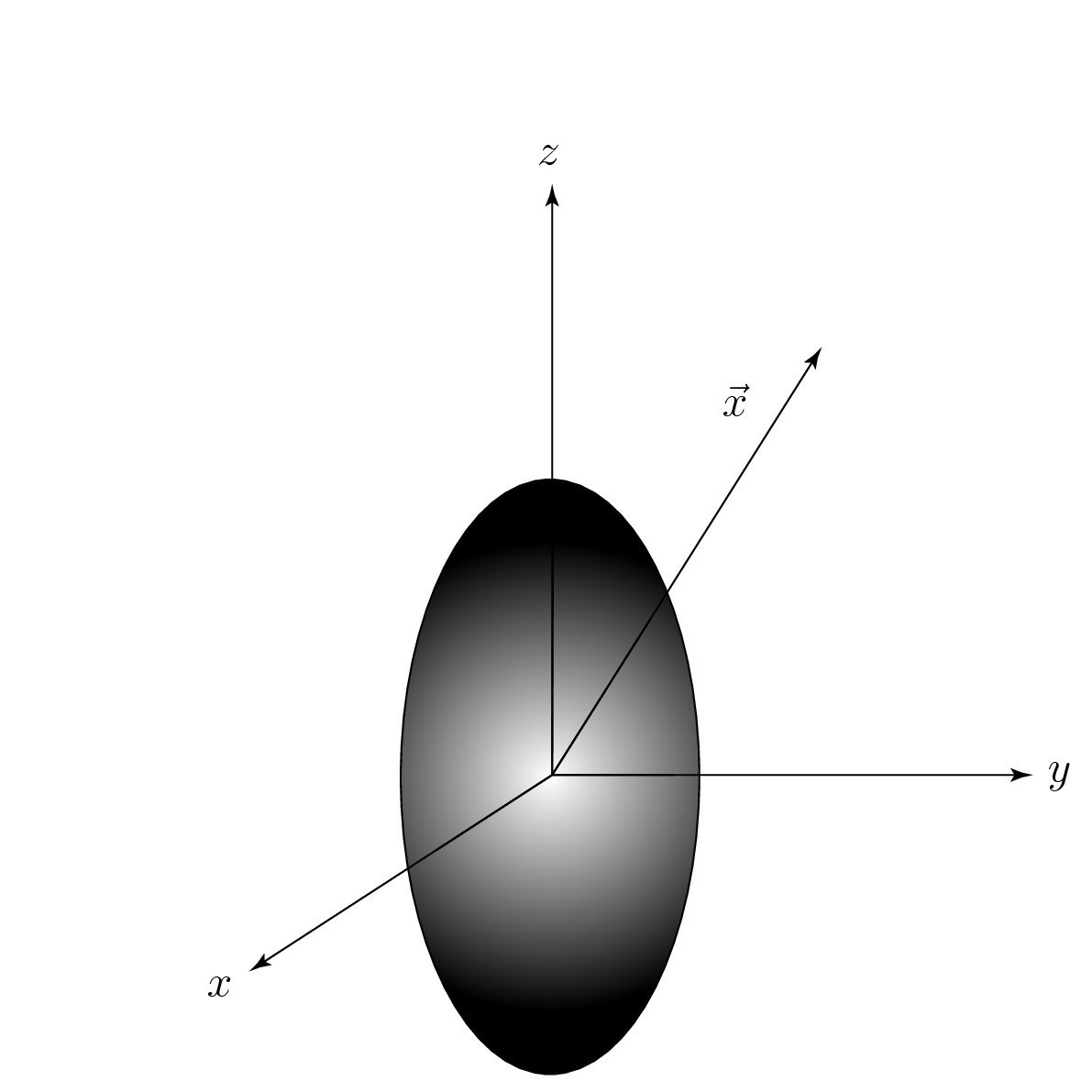
Figure 2: The characteristic diagram for a surface of the GW radiation intensity $\frac{dP_{M}}{d\Sigma}$ in (3.32), as a function of the polar angle $\theta$, showing a prolate ellipsoid geometry in the corresponding intensity profile. Here the binary compact objects reside on the equatorial $x$-$y$ plane as shown in Figure 1(a). Note that, at a given radial distance $r=|\vec{x}|$ from the origin of the binary system of compact objects, the GW radiation intensity on the revolution $z$ axis of the binary compact objects is twice that on the equatorial plane.

Now exploiting (3.23) and (3.28), we find the mass electric field which also includes the mass vector potential effect $\vec{E}_{M}\equiv-\nabla\phi_{M}-\frac{\partial\vec{A}_{M}}{\partial t}=E_{M}^{r}\hat{r}+E_{M}^{\theta}\hat{\theta}+E_{M}^{\phi}\hat{\phi}$ and the mass magnetic one $\vec{B}_{M}\equiv\nabla\times\vec{A}_{M}=B_{M}^{\theta}\hat{\theta}+B_{M}^{\phi}\hat{\phi}$

$$E_{M}^{r} = \frac{2GM\omega}{cr}\left(\sin\left[\omega\left(t-\frac{r}{c}\right)\right]-\cos\left[\omega\left(t-\frac{r}{c}\right)\right]\right),$$

$$E_{M}^{\theta} = cB_{M}^{\phi}=\frac{GM\omega^{2}\delta a}{2c^{2}r}\cos\theta\left(\cos\left[\omega\left(t-\frac{r}{c}\right)\right]\cos\phi+\sin\left[\omega\left(t-\frac{r}{c}\right)\right]\sin\phi\right),$$

$$E_{M}^{\phi} = -cB_{M}^{\theta}=\frac{GM\omega^{2}\delta a}{2c^{2}r}\left(-\cos\left[\omega\left(t-\frac{r}{c}\right)\right]\sin\phi+\sin\left[\omega\left(t-\frac{r}{c}\right)\right]\cos\phi\right),$$ (3.29)

where we have included the relevant leading order terms. Exploiting (3.29), we find $\vec{B}_{M}=\frac{1}{c}(\hat{r}\times\vec{E}_{M})$ which implies that the $\vec{E}_{M}$ and $\vec{B}_{M}$ fields are mutually perpendicular, and are spherical waves (not plane waves) and their amplitudes decrease like $\frac{1}{r}$ as they propagate. However, for large $r$, the GW waves are approximately plane waves over small regions, similar to the EM waves in (A.7) discussed in Appendix A. Note that the $\vec{E}_{M}$ field possesses $E_{M}^{r}\hat{r}$ component originated from the gravitational attraction from the binary compact objects. This characteristic is different from the rotating charge electric dipole moment system where $E_{Q}^{r}\hat{r}$ component vanishes as in (A.7). Note also that, in the GW radiation intensity $\frac{dP_{M}}{d\Sigma}$ in (3.32), we have a vanishing contribution of $E_{M}^{r}\hat{r}$ to $\frac{dP_{M}}{d\Sigma}$ by averaging in time over a complete cycle as shown below.

Next we formulate the mass Poyinting vector in terms of $\vec{E}_{M}$ and $\vec{B}_{M}$ in (3.29)

$$\vec{S}_{M}\equiv\frac{c^{2}}{4\pi G}(\vec{E}_{M}\times\vec{B}_{M})=\frac{c}{4\pi G}\left[(E_{M}^{\perp})^{2}\hat{r}-E_{M}^{r}\vec{E}_{M}^{\perp}\right],$$ (3.30)

where

$$\vec{E}_{M}^{\perp} = E_{M}^{\theta}\hat{\theta}+E_{M}^{\phi}\hat{\phi},$$

$$(E_{M}^{\perp})^{2} = (E_{M}^{\theta})^{2}+(E_{M}^{\phi})^{2}=\left(\frac{GM\omega^{2}\delta a}{2c^{2}r}\right)^{2}\left(1-\sin^{2}\theta\cos^{2}\left[\omega\left(t-\frac{r}{c}\right)-\phi\right]\right).$$ (3.31)

Note that the normalization factor $\frac{c^{2}}{4\pi G}$ in (3.30) is systematically determined by using the proportionality constants $-\frac{G}{c^{2}}$ of $\vec{A}_{M}^{I}$ and $\vec{A}_{M}^{II}$ in (3.25), and $-G$ of $\phi_{M}^{I}$ and $\phi_{M}^{II}$ in (3.21) which is consistent with the Newtonian gravity goldstein80 ; marion04 . Next using (3.30) and (3.31) we find the GW radiation intensity, namely the GW radiation power per surface $\Sigma$, which is obtainable by averaging in time over a complete cycle

$$\frac{dP_{M}}{d\Sigma}\equiv\langle\vec{S}_{M}\rangle=\frac{c}{4\pi G}\left(\frac{GM\omega^{2}\delta a}{2c^{2}r}\right)^{2}\left(1-\frac{1}{2}\sin^{2}\theta\right)\hat{r}.$$ (3.32)

Note that in (3.32) the $\vec{E}_{M}^{\perp}$-component of $\vec{S}_{M}$ in (3.30) vanishes, after averaging in time over a complete cycle and then using $\langle E_{M}^{r}\rangle=0$. Note also that $\frac{dP_{M}}{d\Sigma}$ has a maximum (minimum) value at $\theta=0$ ($\theta=\frac{\pi}{2}$) to yield the invariant relation independent of the radial distance $r$

$$\frac{dP_{M}}{d\Sigma}(\theta=0)=2\frac{dP_{M}}{d\Sigma}\left(\theta=\frac{\pi}{2}\right),$$ (3.33)

implying that, at a given radial distance $r$ from the origin of the binary system of compact objects, the GW radiation intensity on the revolution $z$ axis of the compact objects is twice that on the equatorial $x$-$y$ plane where the compact objects locate. The characteristic invariant in (3.33) also occurs in the EM radiation intensity of the rotating charge electric dipole moment in (A.10). The geometrically invariant surface of the GW radiation intensity $\frac{dP_{M}}{d\Sigma}$ then yields a prolate ellipsoid geometry in the corresponding intensity profile as shown in Figure 2.

The total GW radiation power constructed by integrating $\langle\vec{S}_{M}\rangle$ over a sphere $\Sigma_{r}$ of radius $r$ is then given by

$$P_{M}\equiv\int\langle\vec{S}_{M}\rangle\cdot d\vec{\sigma}=\frac{GM^{2}\omega^{4}(\delta a)^{2}}{6c^{3}},$$ (3.34)

where $d\vec{\sigma}$ is an area element vector perpendicular to the surface $\Sigma_{r}$. As expected, the dimensionality of $P_{M}$ is that of power, which is the same as the dimensionality of $P_{Q}$ in (A.11). This aspect implies that the normalization factor $\frac{c^{2}}{4\pi G}$ in (3.30) is well defined. Note that in the ideal binary compact objects without any distortion ($\delta a=0$) we obtain the vanishing total GW radiation power. In contrast, in the physically merging binary compact objects source we have the total power in (3.34) which is proportional to $(\delta a)^{2}$. Here $\delta a$ is defined in (3.27). These phenomenological aspects are consistent with the second rank tensor approach to the merging binary compact objects wald84 ; hobson06 in the LGR.

Now, it seems appropriate to comment on the second rank tensor approach in the LGR, which is distinct from the MLGR defined in (2.5) and (2.7). For the LGR associated with merging binary compact objects of equal mass $M$ which co-rotate in circular orbits of radius $a$ about their common center of mass with an angular frequency $\omega$ as shown in Figure 1(a), we construct the symmetric second rank tensor for the GW radiation hobson06

$$\bar{h}_{rad}^{00} = 0,~{}~{}~{}\bar{h}_{rad}^{0i}=0,$$

$$\bar{h}^{ij}_{rad} = \frac{8GM\omega^{2}a^{2}}{c^{4}r}\left(\begin{array}[]{ccc}\cos[2\omega(t-r/c)]&\sin[2\omega(t-r/c)]&0\\ \sin[2\omega(t-r/c)]&-\cos[2\omega(t-r/c)]&0\\ 0&0&0\end{array}\right),~{}~{}~{}(i,j=1,2,3).$$ (3.38)

In order to investigate the GW from binary compact objects in the LGR, we introduce the traceless transverse gauge wald84 ; hobson06 , and thus the GW originates from the second rank tensor $\bar{h}_{rad}^{\alpha\beta}$ in (3.38). Note that the GW radiation from the binary compact objects in the MLGR can be described in terms of the mathematically and physically independent vector $\bar{h}^{0\alpha}=-\frac{4}{c}A_{M}^{\alpha}$ in (2.5) and (2.7), without appealing to the second rank tensor $\bar{h}_{rad}^{ij}$ in (3.38) in the LGR. Note also that the graviton possesses spin-one in the MLGR, but spin-two in the LGR, since the MLGR and LGR are delineated in terms of the vector $\bar{h}^{0\alpha}$ related with $\bar{h}^{ij}=0$ in (2.4), and the second rank tensor $\bar{h}_{rad}^{\alpha\beta}$ (especially the non-vanishing space-space components $\bar{h}_{rad}^{ij}$ of the tensor in (3.38)), respectively. Moreover in the LGR the second rank tensor $\bar{h}_{rad}^{ij}$ does not include $(\theta,\phi)$ dependences of $A_{M}^{i}=-\frac{c}{4}\bar{h}^{0i}$ in (3.28) in the MLGR, which are related with those of the GW radiation intensity profile having a prolate ellipsoid geometry in Figure 2.

IV Conclusions

In summary, we have formulated the MLGR where the mass scalar potential has the additional dynamical DOF. In the static gravitational field limit of the MLGR, the mass scalar potential is consistent with the well-established gravitational potential in the Newtonian gravity. Next we also have found that the MLGR allows the mass vector potential which originates from the mass current and is missing in the Newtonian gravity. As an application of the MLGR, we have investigated the phenomenological aspects of the merging binary compact objects which co-rotate in circular orbits about their common center of mass with a constant angular frequency. To be specific, we have constructed the mass scalar and mass vector potentials of the merging binary compact objects at an observation point located far away from the compact objects. We then have formulated the mass electric and mass magnetic fields, and the mass Poyinting vector. Next we have found the GW radiation intensity profile having a prolate ellipsoid geometry due to the merging binary compact objects source, and then explicitly obtained the total GW radiation power due to the source. We also have observed that, in no distorting limit of the binary compact objects, they do not yield the total GW radiation power, which is consistent with the second rank tensor approach in the LGR. One of the main points of this paper is that, in the MLGR we have found the mathematically and physically well defined spin-one graviton, distinct from the second rank tensor approach in the LGR which could allow the spin-two graviton. Note that the status of the graviton existence is still hypothetical. It will be interesting to search for the spin-one graviton which could be related with the well-established spin-one photon phenomenology such as the photoelectric effect and Compton scattering for instance. Once this is done, the MLGR algorithm associated with the graviton could give some progress impacts on the realistic precision astrophysics including the merging binary compact objects phenomenology which is detected in the experimental instruments. Assuming the possibility of the massive spin-one graviton, we have observed that the massive graviton would be interpreted as a GRB-like graviton, which could then be regarded as an anti-graviton. This anti-graviton could be phenomenologically a candidate for an intense radiation flare of the GRB170817A related with the binary compact objects merger event GW170817.

Appendix A EM wave radiation from rotating charge electric dipole moment

In this appendix we pedagogically investigate the charge electric dipole moment jackson99 ; baylis02 ; griffiths99 which possesses charges $+Q$ and $-Q$ rotating on the $x$-$y$ plane. Here the charge electric dipole moment is not merging to yield no distortion. We assume that for simplicity the two charges co-rotate in circular orbits of radius $a$ with an angular frequency $\omega$, as shown in Figure 3. Note that the rotating charge electric dipole can be thought of as the superposition of two oscillating charge electric dipoles, one along the $x$-axis and the other along the $y$-axis griffiths99 . The rotating charge vector $\vec{Q}(t)$ on the $x$-$y$ plane is given by

$$\vec{Q}(t)=Q(\hat{x}\cos\omega t+\hat{y}\sin\omega t).$$ (A.1)

For the charges on the $x$-axis and $y$-axis, exploiting (A.1) we obtain the Green retarded charge scalar potential $\phi_{Q}^{I}$ and $\phi_{Q}^{II}$, respectively

$$\phi_{Q}^{I}(\vec{x},t) = \frac{1}{4\pi\epsilon_{0}}\left(\frac{Q\cos[\omega(t-R_{+}/c)]}{R_{+}}-\frac{Q\cos[\omega(t-R_{-}/c)]}{R_{-}}\right),$$

$$\phi_{Q}^{II}(\vec{x},t) = \frac{1}{4\pi\epsilon_{0}}\left(\frac{Q\sin[\omega(t-\bar{R}_{+}/c)]}{\bar{R}_{+}}-\frac{Q\sin[\omega(t-\bar{R}_{-}/c)]}{\bar{R}_{-}}\right),$$ (A.2)

where $R_{\pm}$ and $\bar{R}_{\pm}$ are given by (3.22). Here the subscript $Q$ stands for the charge related quantities. Following the technical procedures in Section 3, we find the total contributions to the charge scalar potentials $\phi_{Q}=\phi_{Q}^{I}+\phi_{Q}^{II}$

$$\phi_{Q}(\vec{x},t)=-\frac{Q\omega a}{2\pi\epsilon_{0}}\left(\frac{\sin\theta}{cr}\right)\left(\cos\phi\sin\left[\omega\left(t-\frac{r}{c}\right)\right]-\sin\phi\cos\left[\omega\left(t-\frac{r}{c}\right)\right]\right),$$ (A.3)

where we have used approximations $a\ll r$ and $\frac{1}{r}\ll\frac{\omega}{c}$, implying that the wavelength $\lambda\left(=\frac{2\pi c}{\omega}\right)$ of the EM wave is much smaller than $r$ to yield $\lambda\ll r$.

Figure 3: The schematic diagram for a rotating charge electric dipole moment consisting of charges $+Q$ and $-Q$ which co-rotate in circular orbits of radius $a$, with an angular frequency $\omega$.

Making use of (A.1) for the charges co-rotating on the $x$-$y$ plane, we find the charge current

$$\vec{I}_{Q}(t)=-Q\omega(\hat{x}\sin\omega t-\hat{y}\cos\omega t).$$ (A.4)

Next we find the retarded charge vector potentials $\vec{A}_{Q}^{I}$ and $\vec{A}_{Q}^{II}$ for the charge currents on the $x$-axis and the $y$-axis, respectively

$$\vec{A}_{Q}^{I}(\vec{x},t) = \frac{\mu_{0}Q\omega}{4\pi}\left(-\int_{-a}^{0}\frac{\sin[\omega(t-R_{-}^{\prime}/c)]}{R_{-}^{\prime}}dx^{\prime}-\int_{0}^{a}\frac{\sin[\omega(t-R_{+}^{\prime}/c)]}{R_{+}^{\prime}}dx^{\prime}\right)\hat{x},$$

$$\vec{A}_{Q}^{II}(\vec{x},t) = \frac{\mu_{0}Q\omega}{4\pi}\left(\int_{-a}^{0}\frac{\cos[\omega(t-\bar{R}_{-}^{\prime}/c)]}{\bar{R}_{-}^{\prime}}dy^{\prime}+\int_{0}^{a}\frac{\cos[\omega(t-\bar{R}_{+}^{\prime}/c)]}{\bar{R}_{+}^{\prime}}dy^{\prime}\right)\hat{y},$$ (A.5)

where $R_{\pm}^{\prime}$ and $\bar{R}_{\pm}^{\prime}$ are given by (3.26). Here we have used the approximations $a\ll r$ and $\frac{1}{r}\ll\frac{\omega}{c}$. Note that in (A.2) and (A.5) we have used the charges $(+Q,-Q)$, distinct form the binary system of compact objects where we have exploited the masses $(M,M)$ in (3.21) and (3.25). Exploiting the charge vector potentials in (A.5), we obtain the total retarded charge vector potential $\vec{A}_{Q}=\vec{A}_{Q}^{I}+\vec{A}_{Q}^{II}$

$$\vec{A}_{Q}(\vec{x},t) = \frac{\mu_{0}Q\omega a}{2\pi r}\left[-\left(\sin\left[\omega\left(t-\frac{r}{c}\right)\right]+\frac{\omega a}{2c}\sin\theta\cos\phi\cos\left[\omega\left(t-\frac{r}{c}\right)\right]\right)\hat{x},\right.$$ (A.6)

$$\left.+\left(\cos\left[\omega\left(t-\frac{r}{c}\right)\right]-\frac{\omega a}{2c}\sin\theta\sin\phi\sin\left[\omega\left(t-\frac{r}{c}\right)\right]\right)\hat{y}\right].$$

Now using (A.3) and (A.6), we find the charge electric field $\vec{E}_{Q}\equiv-\nabla\phi_{Q}-\frac{\partial\vec{A}_{Q}}{\partial t}=E_{Q}^{\theta}\hat{\theta}+E_{Q}^{\phi}\hat{\phi}$ and charge magnetic one $\vec{B}_{Q}\equiv\nabla\times\vec{A}_{Q}=B_{Q}^{\theta}\hat{\theta}+B_{Q}^{\phi}\hat{\phi}$

$$E_{Q}^{\theta} = cB_{Q}^{\phi}=\frac{\mu_{0}Q\omega^{2}a}{2\pi r}\cos\theta\left(\cos\left[\omega\left(t-\frac{r}{c}\right)\right]\cos\phi+\sin\left[\omega\left(t-\frac{r}{c}\right)\right]\sin\phi\right),$$

$$E_{Q}^{\phi} = -cB_{Q}^{\theta}=\frac{\mu_{0}Q\omega^{2}a}{2\pi r}\left(-\cos\left[\omega\left(t-\frac{r}{c}\right)\right]\sin\phi+\sin\left[\omega\left(t-\frac{r}{c}\right)\right]\cos\phi\right),$$ (A.7)

where we have included the relevant leading terms. From (A.7), we obtain $\vec{B}_{Q}=\frac{1}{c}(\hat{r}\times\vec{E}_{Q})$. Note that $\vec{E}_{Q}$ does not have the $E_{Q}^{r}$ component, different form the $\vec{E}_{M}$ of the binary compact objects which possesses the $E_{M}^{r}$ component in (3.29).

Next we formulate the charge Poyinting vector in terms of $\vec{E}_{Q}$ and $\vec{B}_{Q}$ in (A.7)

$$\vec{S}_{Q}\equiv\frac{1}{\mu_{0}}(\vec{E}_{Q}\times\vec{B}_{Q})=\frac{1}{\mu_{0}c}(E_{Q})^{2}\hat{r}$$ (A.8)

where

$$(E_{Q})^{2}=(E_{Q}^{\theta})^{2}+(E_{Q}^{\phi})^{2}=\left(\frac{\mu_{0}Q\omega^{2}a}{2\pi r}\right)^{2}\left(1-\sin^{2}\theta\cos^{2}\left[\omega\left(t-\frac{r}{c}\right)-\phi\right]\right).$$ (A.9)

Next, using (A.8) and (A.9) and averaging in time over a complete cycle, we arrive at the EM radiation intensity, namely the EM radiation power per surface $\Sigma$

$$\frac{dP_{Q}}{d\Sigma}\equiv\langle\vec{S}_{Q}\rangle=\frac{1}{\mu_{0}c}\left(\frac{\mu_{0}Q\omega^{2}a}{2\pi r}\right)^{2}\left(1-\frac{1}{2}\sin^{2}\theta\right)\hat{r}.$$ (A.10)

Note that the total EM radiation power constructed by integrating $\langle\vec{S}_{Q}\rangle$ over a sphere $\Sigma_{r}$ of radius $r$ is given by

$$P_{Q}\equiv\int\langle\vec{S}_{Q}\rangle\cdot d\vec{\sigma}=\frac{2\mu_{0}Q^{2}\omega^{4}a^{2}}{3\pi c},$$ (A.11)

where $d\vec{\sigma}$ is an area element vector perpendicular to the surface $\Sigma_{r}$. Note that the total EM radiation power $P_{Q}$ in (A.11) for the rotating charge electric dipole moment on the $x$-$y$ plane is twice that for the oscillating charge electric dipole moment along the $x$-direction, assuming the same time dependence possessing an angular frequency $\omega$ of these rotating and oscillating cases.

References

- (1) R.M. Wald, General Relativity (University of Chicago Press, Chicago, 1984).
- (2) M.P. Hobson, G. Efstathiou and A.N. Lasenby, General Relativity: An Introduction for Physicists (University of Chicago Press, Chicago, 2006).
- (3) M. Fierz and W. Pauli, Relativistic wave equations for particles of arbitrary spin in an electromagnetic field, Proc. Roy. Soc. Lond. A 173, 211 (1939).
- (4) J. Aasi et al. [LIGO Scientific Collaboration], Advanced LIGO, Class. Quant. Grav. 32, 074001 (2015), arXiv:1411.4547.
- (5) D. Reitze et al., Cosmic explorer: the U.S. contribution to gravitational-wave astronomy beyond LIGO, Bull. Am. Astron. Soc. 51, 35 (2019), arXiv:1907.04833.
- (6) S. Jana, S.J. Kapadia, T. Venumadhav and P. Ajith, Cosmography using strongly lensed gravitational waves from binary black holes, Phys. Rev. Lett. 130, 261401 (2023), arXiv:2211.12212.
- (7) R.W. Klebesadel, I.B. Strong and R.A. Olson, Observations of gamma-ray bursts of cosmic origin, Astrophys. J. Lett. 182, L85 (1973).
- (8) D. Svinkin et al., A bright gamma-ray flare interpreted as a giant magnetar flare in NGC 253, Nature 589, 211 (2021), arXiv:2101.05104.
- (9) S.T. Hong, Dirac type relativistic quantum mechanics for massive photons, Nucl. Phys. B 980, 115852 (2022), arXiv:2108.07299.
- (10) R.A. Hulse and J.H. Taylor, Discovery of a pulsar in a binary system, Astrophys. J. Lett. 195, L51 (1975).
- (11) B.P. Abbott et al. [LIGO Scientific and Virgo Collaborations], GW170817: Observation of gravitational waves from a binary neutron star inspiral, Phys. Rev. Lett. 119, 161101 (2017), arXiv:1710.05832.
- (12) B.P. Abbott et al. [LIGO Scientific and Virgo and Fermi-GBM and INTEGRAL Collaborations], Gravitational waves and gamma-rays from a binary neutron star merger: GW170817 and GRB 170817A, Astrophys. J. Lett. 848, L13 (2017), arXiv:1710.05834.
- (13) A. Goldstein et al., An ordinary short gamma-ray burst with extraordinary implications: fermi-GBM detection of GRB 170817A, Astrophys. J. Lett. 848, L14 (2017), arXiv:1710.05446.
- (14) V.M. Kaspi and A. Beloborodov, Magnetars, Ann. Rev. Astron. Astrophys. 55, 261 (2017), arXiv:1703.00068.
- (15) R. Abbott et al. [LIGO Scientific and VIRGO and KAGRA Collaborations], Search for gravitational-wave transients associated with magnetar bursts in Advanced LIGO and Advanced Virgo data from the third observing run, (2022), arXiv:2210.10931.
- (16) H. Goldstein, Classical Mechanics (Addison-Wesley, London, 1980).
- (17) S.T. Thornton and J.B. Marion, Classical Dynamics of Particles and Systems (Thomson, Belmont, 2004).
- (18) N.W. Ashcroft and N.D. Mermin, Solid State Physics (Brooks/Cole, London, 1976).
- (19) S.T. Hong, Photon intrinsic frequency and size in stringy photon model, Nucl. Phys. B 976, 115720 (2022), arXiv:2111.11852.
- (20) J.D. Jackson, Classical Electrodynamics (John Wiley & Sons, Danvers, 1999).
- (21) W.E. Baylis, Electrodynamics: A Modern Geometric Approach (Birkhäuser, Boston, 2002).
- (22) D.J. Griffiths, Introduction to Electrodynamics (Prentice Hall, Upper Saddle River, 1999).