Spatial clustering of temporal energy profiles with empirical orthogonal functions and max-p regionalization

Abstract

This paper presents a spatial clustering method to create regions with similar time-varying energy characteristics. This method combines empirical orthogonal functions (EOFs) for dimensionality reduction and max-p regionalization for spatial clustering. The proposed approach creates regions that each have a similar value of a spatially extensive attribute, such as available land area, population, or GDP, as well as similar weather-dependent temporal energy profiles, such as wind and solar generation potential or heating and cooling demand, within each region. We demonstrate this technique using hourly wind and solar generation potential in 2019 in Ireland and Britain. Solar generation clusters are best-defined at a smaller land area threshold compared to wind generation.

1 Introduction

This paper addresses the question: How can spatiotemporal energy data be used to create regions of similar size with similar time-varying energy characteristics? We propose a spatial clustering method that combines empirical orthogonal functions (EOFs) for dimensionality reduction of temporal data and max-p regionalization for spatial clustering to address this problem.

As electricity systems become increasingly reliant on weather [1], incorporating high spatial and temporal resolution data into energy systems modeling is necessary. One of the primary approaches for incorporating higher spatial and temporal resolution data into energy systems modeling while maintaining computational tractability is spatial clustering to create regions with representative energy characteristics. Two widely used methods for spatial clustering of energy data are k-means clustering [2, 3, 4, 5, 6, 7, 8, 9] and max-p regionalization [2, 4, 10, 11]. These spatial clustering techniques are most commonly used on static spatial data, such as total annual energy demand or annual wind and solar potential [3, 4, 5, 10, 6, 7, 11].

These approaches based on static spatial data do not account for temporal differences in energy data within regions. To address this issue, a few works have proposed methods for spatial clustering of temporal energy data. Getman et al. [2] compare the use of k-means clustering and max-p regionalization of reduced temporal data to create regions with similar solar potential. More recently, Jani et al. [9] use k-means clustering to group areas with similar correlation coefficients for wind and solar to identify locations with complementary renewable potential, and Frysztacki et al. [8] propose the use of hierarchical agglomerative clustering of wind and solar potential to create regions for energy systems planning.

Using k-means clustering on temporal can result in regions of different sizes, for instance, areas with different annual renewable potential or annual demand. In this paper, we propose a spatial clustering method that combines EOFs for dimensionality reduction and max-p regionalization to create regions with similar time-varying energy characteristics where all regions have similar values of another spatially extensive attribute. This approach can be helpful in ensuring that all clustered regions represent a significant supply or demand potential.

2 Data and methods

In this section, we discussion the data used to demonstrate this spatial clustering technique and detail the EOF analysis and max-p regionalization approach it uses.

2.1 Data

We demonstrate the proposed clustering technique using hourly onshore wind and solar generation potential in 2019 in Ireland and Britain at 0.3 degree by 0.3 degree spatial resolution (approximately 30 km by 30 km). We use the Python package atlite [12] to calculate the generation potential for a Vestas V90 3MW wind turbine and a crystalline silicon photovoltaic based on reanalysis data from ERA5 [13].

2.2 EOF analysis

We use empirical orthogonal function (EOF) analysis for dimensionality reduction of wind and solar data prior to spatial clustering. EOF analysis is used in meteorology, oceanography, and climate science to identify key spatial patterns in spatiotemporal data. This technique involves calculating the eigenvalues and eigenvectors of a spatially weighted anomaly covariance matrix of a spatiotemporal field [14]. This procedure decomposes spatiotemporal data into a set of principal component (PC) time series and corresponding EOF spatial patterns, which capture the correlation between each the PC and the time series at each point in space.

We use the eofs python package [15] to perform EOF analysis on 1 year of hourly wind and solar generation data in Britain and Ireland in 2019. Because wind and solar generation potential are weather-driven, we expect that the first few PCs will capture most of the variance, as with weather processes [14]. We will limit our analysis to only the PCs and EOFs that account for greater than 1% of the total variance.

2.3 Max-p regionalization

The max-p regions problem seeks to maximize the number of spatially contiguous regions that meet a certain threshold value, in this case land area, while minimizing heterogeneity of features within a region, in this case the EOF correlation values [16]. We apply max-p regionalization to the first 5 wind EOF values and the first 4 solar EOF values to create wind and solar regions. This means that each clustered region should have similar temporal variation in generation potential, as well as comparable total annual generation.

We use the spopt Python library [17, 18] to perform max-p regionalization. Because the exact max-p regions problem is NP-hard, this library implements the heuristic approach introduced by Wei et al. [19]. For both the wind and solar EOFs, max-p regionalization is performed with area threshold values of 50,000, 70,000, and 100,000 km² to generate different sets of wind and solar regions with similar values of total annual generation. Rook contiguity is used for the contiguity constraint, so each spatial area within a region must share an edge with another area in that region.

2.4 Cluster evaluation

To evaluate the clusters resulting from this process, we use the Python library scikit-learn [20] to calculate the Silhouette Coefficient [21] using cityblock distance based on the underlying hourly renewable potential. This metric compares the mean distance between a sample and all other points in the same cluster, with the mean distance between a sample and all points in the next nearest cluster, so scores closer to 1 indicate more well-defined clusters.

3 Results

In this section, we discuss the results of the EOF analysis and max-p regionalization clustering for the solar and wind data.

3.1 EOF analysis

As expected for weather-driven quantities, the first few EOFs and PCs account for a large share of variance in the wind and solar generation potential. As shown in Figure 1(a), the first 5 EOFs account for 80% of variance in onshore wind potential in Britain and Ireland, and the sixth EOF accounts for less than 1% of variance. The first 4 EOFs account for 91% of variance in onshore solar potential, shown in Figure 1(b), and the fifth EOF accounts for less than 1% of variance. We therefore limit our analysis to the first 5 EOFs for wind and the first 4 EOFs for solar.

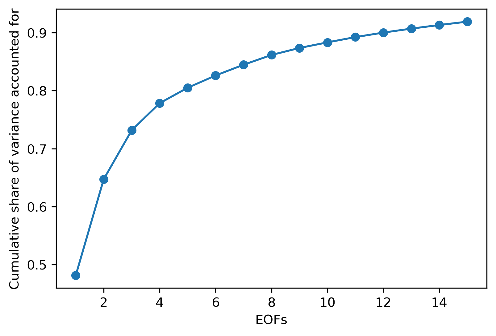
(a) Wind variance vs. EOFs

(b) Solar variance vs. EOFs

Figure 1: Cumulative share of wind and solar variance accounted for with each EOF and its corresponding PC.

The leading five EOFs for wind power in Britain, Ireland, and the surrounding areas are shown in Figure 2. Almost half of the variance in wind is captured in the first EOF, shown in Figure 2(a), which is highly and postively correlated with the entire area. North-south and east-west patterns account for the next highest shares in wind potential (Figures 2(b) and 2(c)), followed by coastal vs. inland patterns (Figures 2(d) and 2(e)).

(a) EOF 1

(b) EOF 2

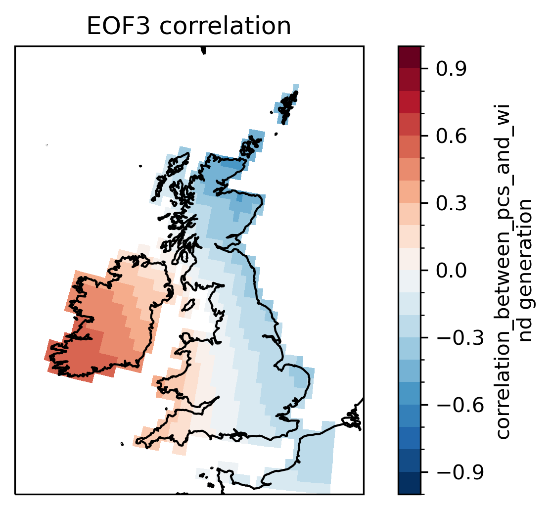
(c) EOF 3

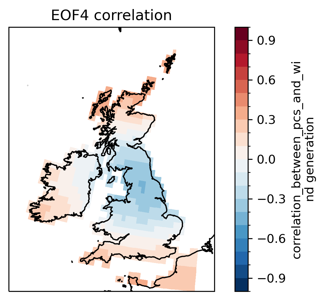
(d) EOF 4

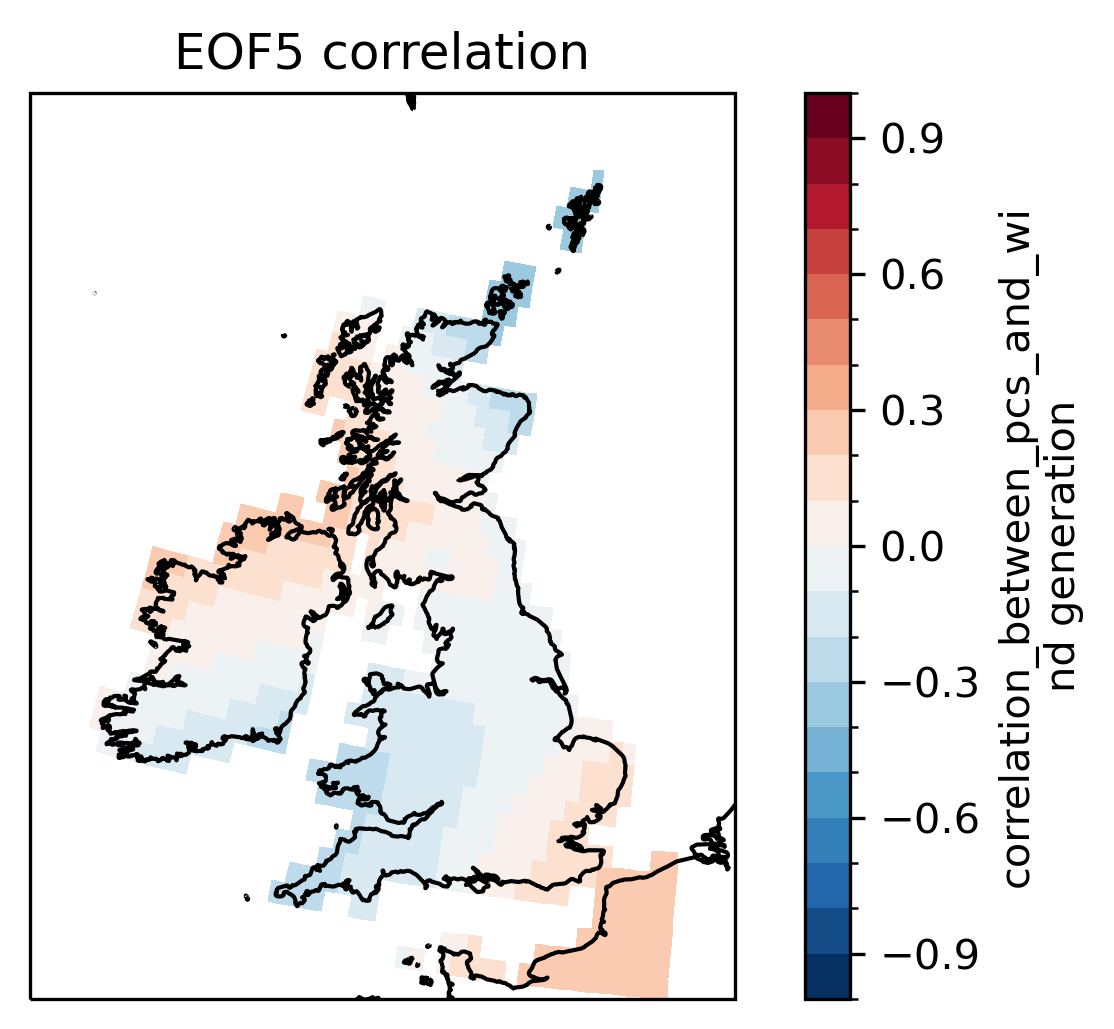
(e) EOF 5

Figure 2: The leading five EOFs for wind power in Britain, Ireland, and surrounding areas.

The leading four EOFs for solar generation potential are shown in Figure 3. Over 80% of solar variation is captured in the first EOF, shown in Figure 3(a). The corresponding PC captures seasonal and diurnal patterns as well as large storm systems that effect solar generation in the entire region. The following three EOFs capture northeast-southwest (Figure 3(b)), east-west (Figure 3(c), and coastal-inland patterns (Figure 3(d)).

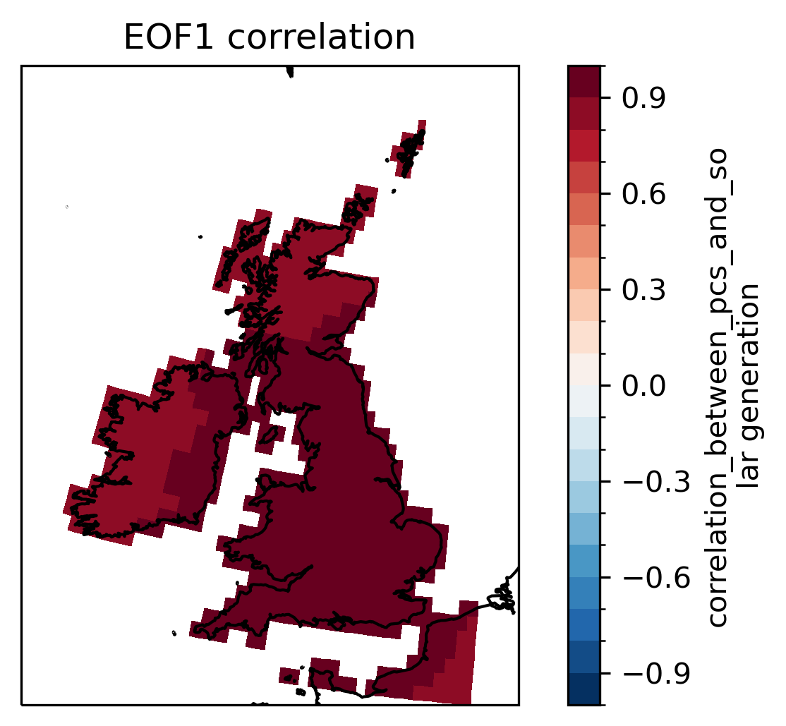
(a) EOF 1

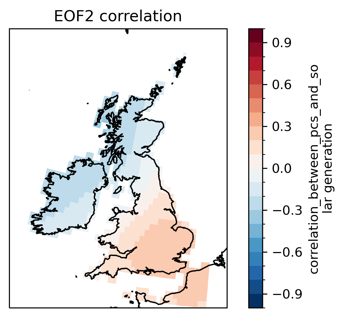
(b) EOF 2

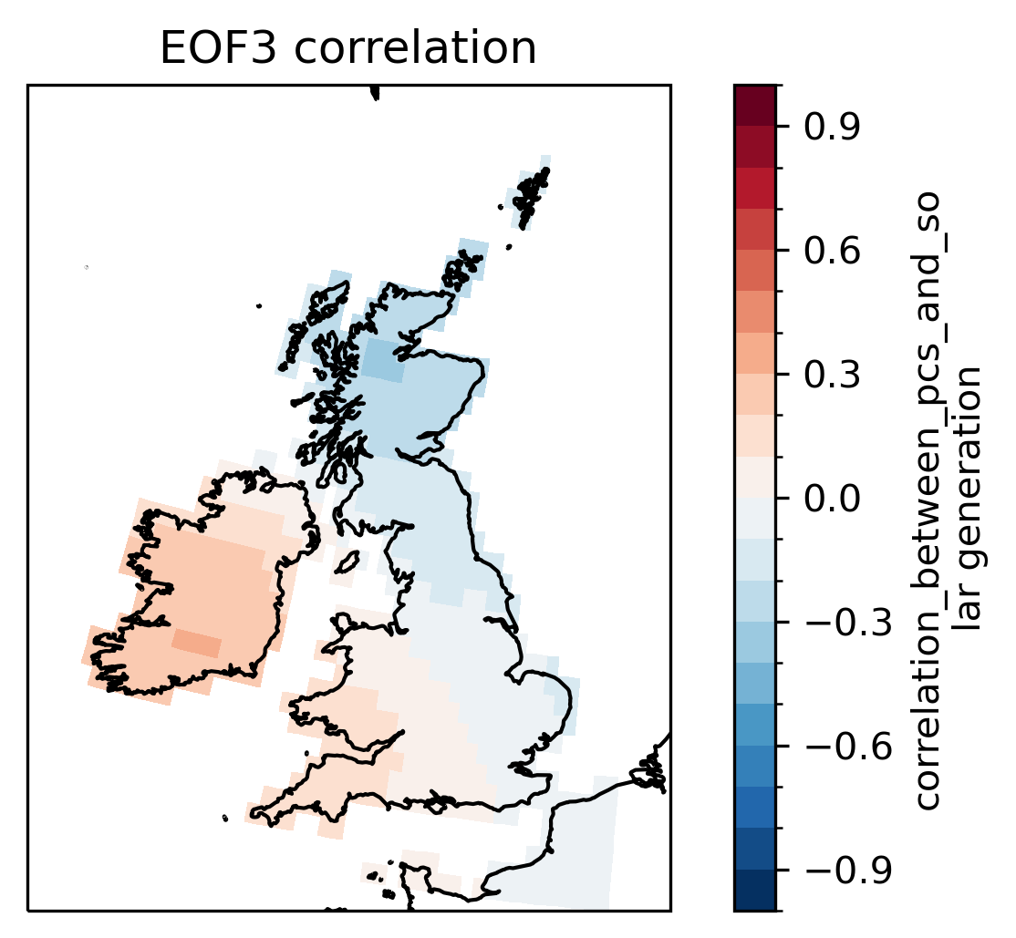
(c) EOF 3

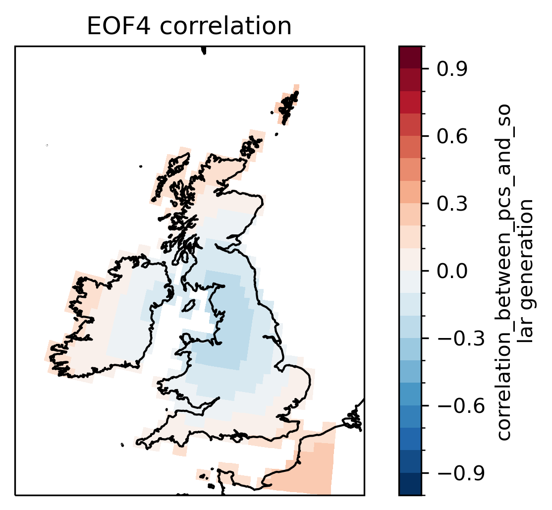
(d) EOF 4

Figure 3: The leading four EOFs for photovoltaic power in Britain, Ireland, and surrounding areas.

3.2 Max-p regionalization

The clustered wind regions and sample generation patterns are shown in Figure 4. Clustered regions are shown in Figures 4(a), 4(c), and 4(e). As the land area threshold increases, regional boundaries capture wind generation differences between Ireland and Britain, as well as north-south differences in Britain.

The sample generation patterns in Figures 4(b), 4(d), and 4(f) display the median wind profile for each region for 14 to 16 September, with the range from the 25th to 75th percentile values filled. These profiles show that areas within a clustered region generally have similar temporal patterns in wind generation even as the range of generation values increases with larger threshold values. The Silhouette Cofficients range from 0.153 for the 50,000 km² land area threshold to 0.179 for the largest land area threshold of 100,000 km². These near-zero values indicate that there is overlap between wind generation potential in the regions, as expected for adjacent regions.

(a) 50,000 km² threshold regions

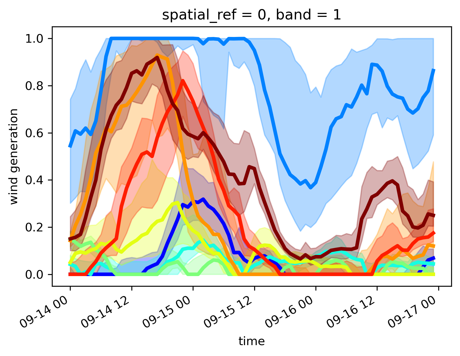
(b) 50,000 km² threshold generation, Silhouette: 0.153

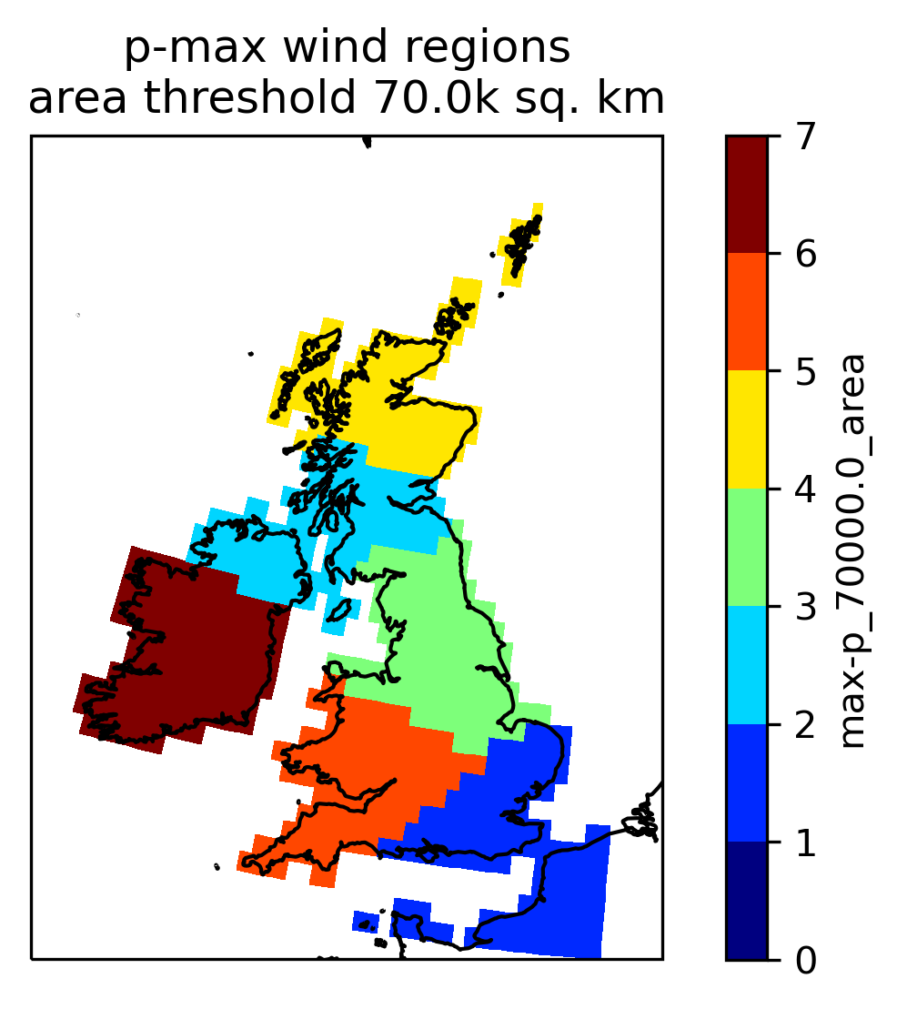
(c) 70,000 km² threshold regions

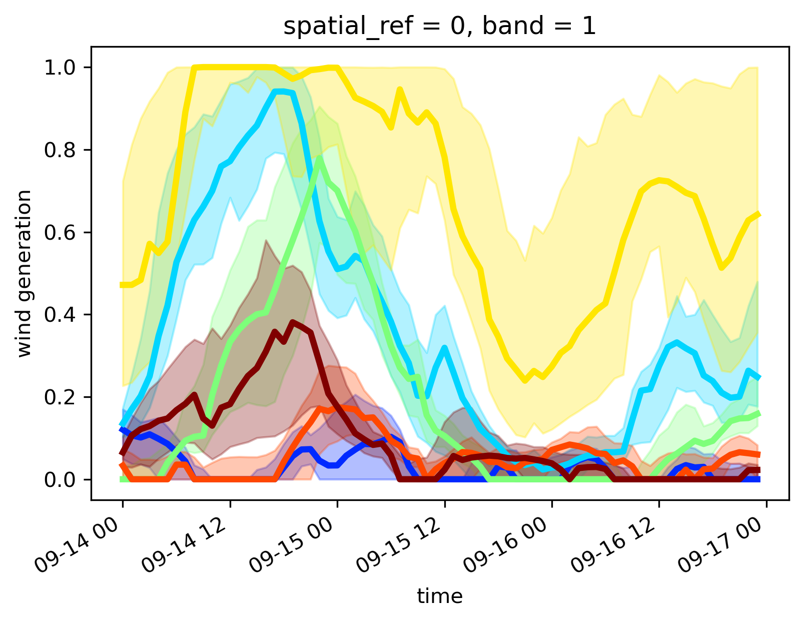
(d) 70,000 km² threshold generation, Silhouette: 0.175

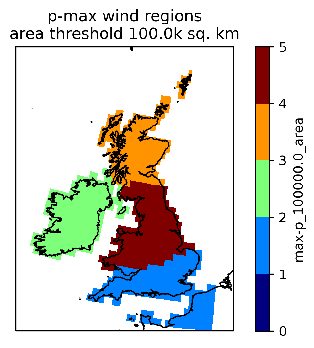
(e) 100,000 km² threshold regions

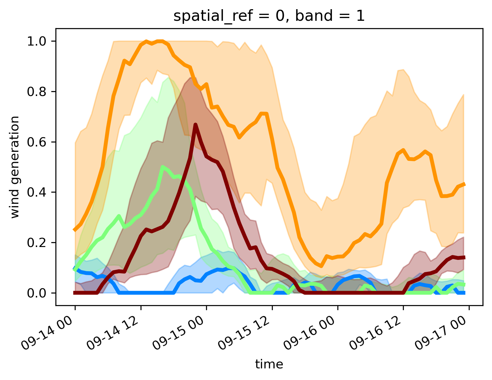
(f) 100,000 km² threshold generation, Silhouette: 0.179

Figure 4: Wind regions for area thresholds from 50,000 km² to 100,000 km² in Britain, Ireland, and surrounding areas and median, 25th, and 75th percentile generation profiles for 14 to 16 September.

The clustered solar regions and sample generation patterns are shown in Figure 5. Compared to the wind regions in Figure 4, these regions capture more east-west differences in solar potential.

Sample solar generation patterns for 06:00 to 20:00 on 2 March are shown in Figures 5(b), 5(d), and 5(f). Although there are large ranges between the 25th and 75th percentile values for each time, areas within each cluster have similar temporal patterns in solar potential and tend to peak at similar times. The Silhouette Coefficients range from 0.125 for the 50,000 km² land area threshold to 0.169 for the 70,000 km² land area threshold. Like the wind generation profiles, these near-zero values indicate overlap between the solar profiles in each cluster. The largest Silhouette Coefficient occurs at a smaller spatial scale of 70,000 km², compared to the wind profiles, where the largest Silhouette Coefficient occurred at the largest land area threshold considered.

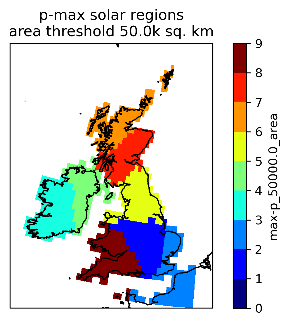
(a) 50,000 km² threshold regions

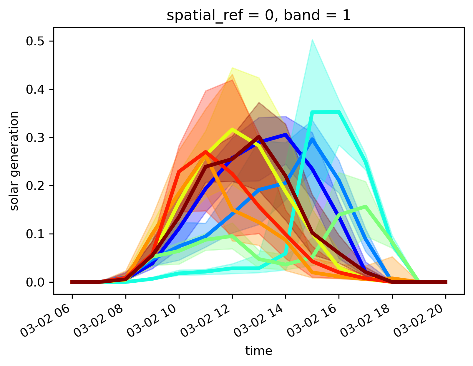
(b) 50,000 km² threshold generation, Silhouette: 0.125

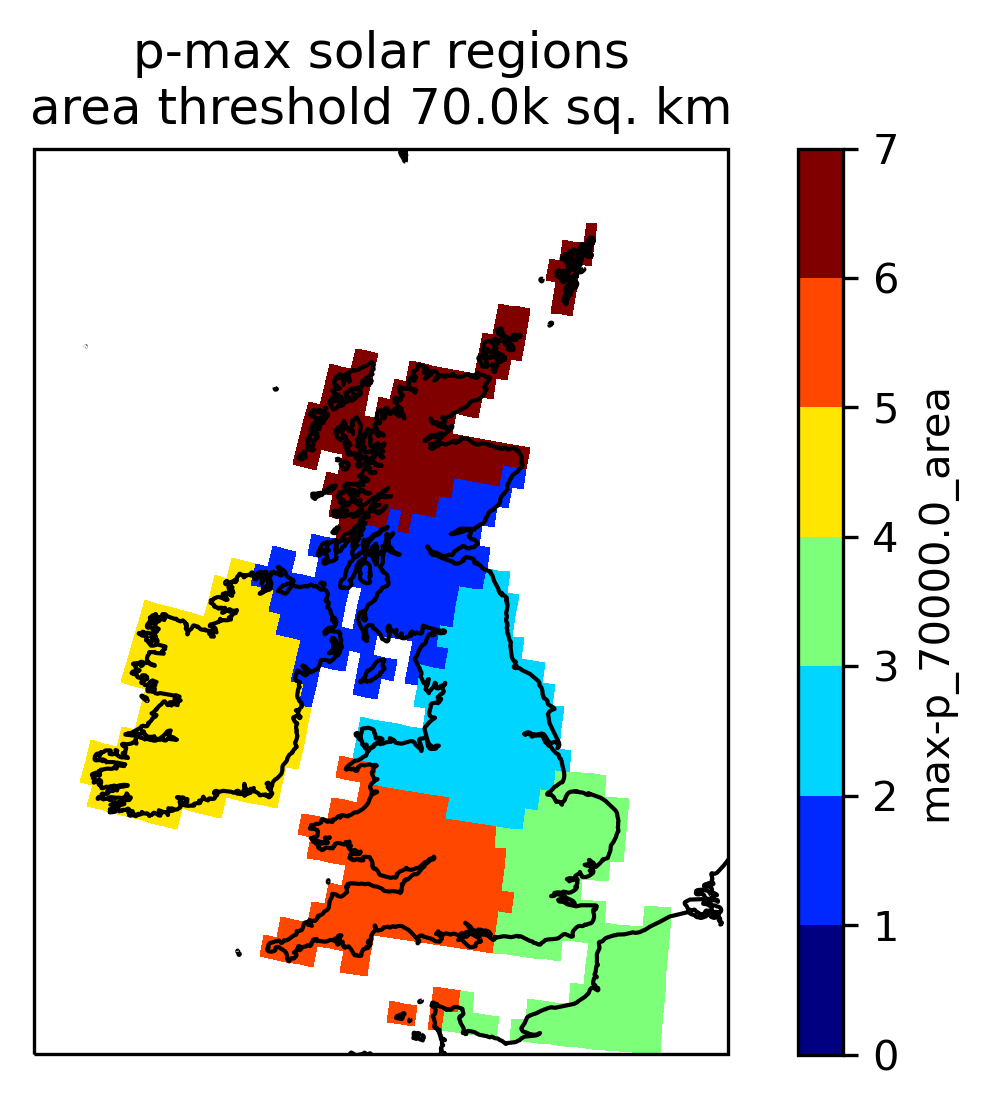
(c) 70,000 km² threshold regions

(d) 70,000 km² threshold generation, Silhouette: 0.169

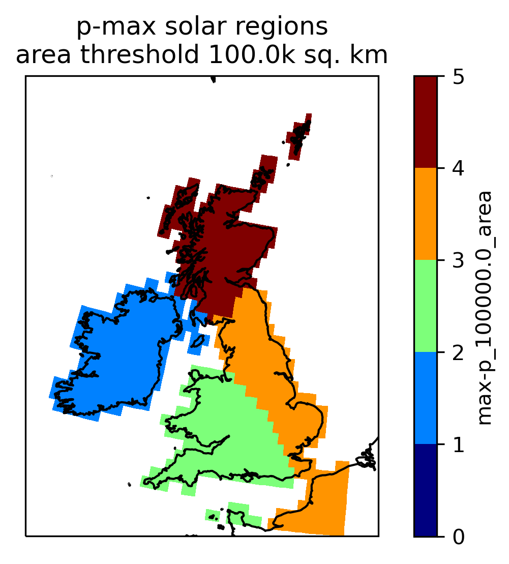
(e) 100,000 km² threshold regions

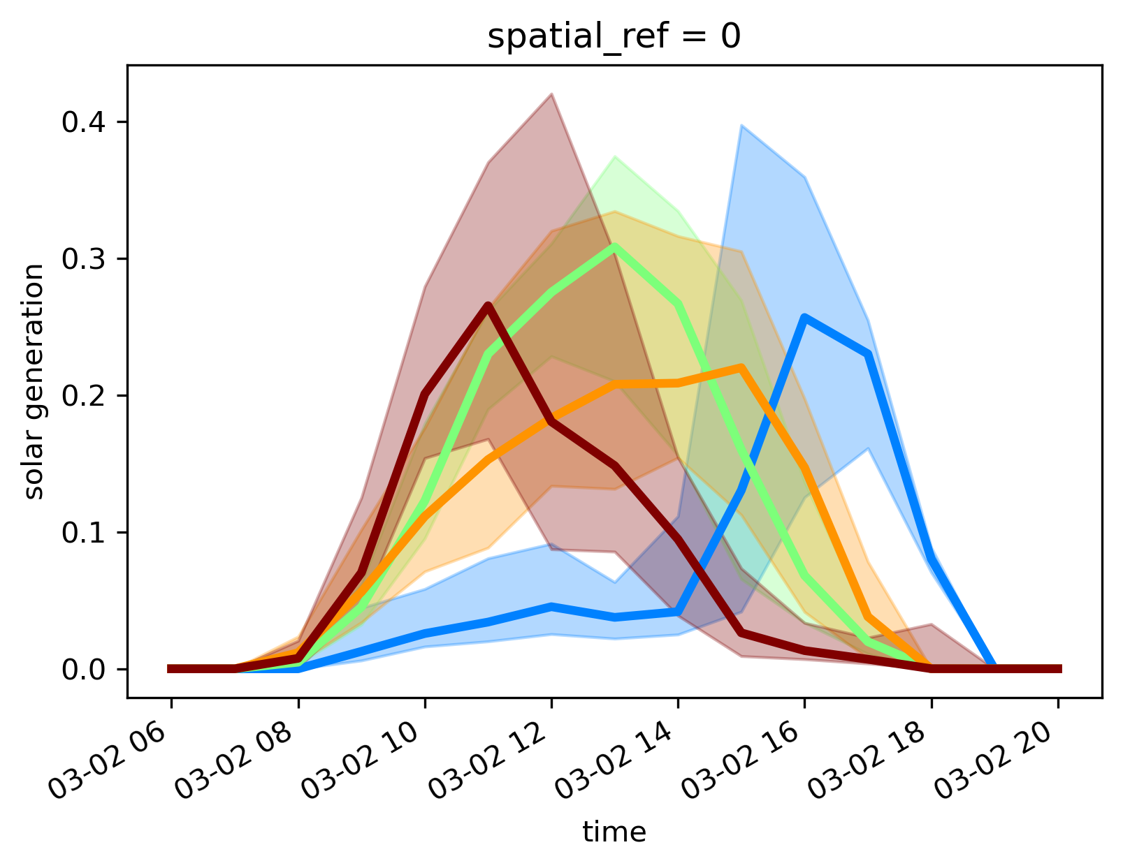
(f) 100,000 km² threshold regions, Silhouette: 0.154

Figure 5: Solar regions for area thresholds from 50,000 km² to 100,000 km² in Britain, Ireland, and surrounding areas and median, 25th, and 75th percentile generation profiles for 6:00 to 20:00 on 2 March.

4 Conclusion

We introduce a method for identifying areas with similar temporal energy profiles by combining EOF analysis with max-p regionalization. We demonstrate this method for a case study of hourly wind and solar potential in 2019 in Britain and Ireland and show that this technique creates regions with similar wind and solar potential profiles. Of the land area thresholds considered, regions with a threshold of 100,000 km² had the best Silhouette Coefficient for the wind generation profiles and regions with a threshold of 70,000 km² had the best Silhouette Coefficient for solar generation profiles, indicating better-defined clusters occur at smaller spatial scales for solar generation compared to wind generation.

References

- [1] I. Staffell and S. Pfenninger, “The increasing impact of weather on electricity supply and demand,” Energy, vol. 145, pp. 65–78, Feb. 2018.
- [2] D. Getman, A. Lopez, T. Mai, and M. Dyson, “Methodology for Clustering High-Resolution Spatiotemporal Solar Resource Data,” Tech. Rep. NREL/TP-6A20–63148, 1225896, Sept. 2015.
- [3] J. Horsch and T. Brown, “The role of spatial scale in joint optimisations of generation and transmission for European highly renewable scenarios,” in 2017 14th International Conference on the European Energy Market (EEM), (Dresden, Germany), pp. 1–7, IEEE, June 2017.
- [4] K. Siala and M. Y. Mahfouz, “Impact of the choice of regions on energy system models,” Energy Strategy Reviews, vol. 25, pp. 75–85, Aug. 2019.
- [5] C. Scaramuzzino, G. Garegnani, and P. Zambelli, “Integrated approach for the identification of spatial patterns related to renewable energy potential in European territories,” Renewable and Sustainable Energy Reviews, vol. 101, pp. 1–13, Mar. 2019.
- [6] M. Frysztacki and T. Brown, “Modeling Curtailment in Germany: How Spatial Resolution Impacts Line Congestion,” in 2020 17th International Conference on the European Energy Market (EEM), (Stockholm, Sweden), pp. 1–7, IEEE, Sept. 2020.
- [7] M. M. Frysztacki, J. Hörsch, V. Hagenmeyer, and T. Brown, “The strong effect of network resolution on electricity system models with high shares of wind and solar,” Applied Energy, vol. 291, p. 116726, June 2021.
- [8] M. M. Frysztacki, G. Recht, and T. Brown, “A comparison of clustering methods for the spatial reduction of renewable electricity optimisation models of Europe,” Energy Informatics, vol. 5, p. 4, May 2022.
- [9] H. K. Jani, S. S. Kachhwaha, G. Nagababu, and A. Das, “Temporal and spatial simultaneity assessment of wind-solar energy resources in India by statistical analysis and machine learning clustering approach,” Energy, vol. 248, p. 123586, June 2022.
- [10] C. E. Fleischer, “Minimising the effects of spatial scale reduction on power system models,” Energy Strategy Reviews, vol. 32, p. 100563, Nov. 2020.
- [11] C. E. Fleischer, “Using the max-p regions problem algorithm to define regions for energy system modelling,” MethodsX, vol. 8, p. 101211, 2021.
- [12] F. Hofmann, J. Hampp, F. Neumann, T. Brown, and J. Horsch, “atlite: A Lightweight Python Package for Calculating Renewable Power Potentials and Time Series,” Journal of Open Source Software, vol. 6, no. 62, p. 3294, 2021.
- [13] Copernicus European Centre for Medium-Range Weather Forecasts, “ERA5 dataset,” 2022.
- [14] “The Climate Data Guide: Empirical Orthogonal Function (EOF) Analysis and Rotated EOF Analysis.”
- [15] A. Dawson, “eofs: A Library for EOF Analysis of Meteorological, Oceanographic, and Climate Data,” Journal of Open Research Software, vol. 4, p. 14, Apr. 2016.
- [16] J. C. Duque, L. Anselin, and S. J. Rey, “The Max-P-Regions Problem,” Journal of Regional Science, vol. 52, no. 3, pp. 397–419, 2012.
- [17] X. Feng, J. D. Gaboardi, E. Knaap, S. J. Rey, and R. Wei, “pysal/spopt,” Jan. 2021.
- [18] X. Feng, G. Barcelos, J. D. Gaboardi, E. Knaap, R. Wei, L. J. Wolf, Q. Zhao, and S. J. Rey, “spopt: a python package for solving spatial optimization problems in PySAL,” Journal of Open Source Software, vol. 7, no. 74, p. 3330, 2022.
- [19] R. Wei, S. Rey, and E. Knaap, “Efficient regionalization for spatially explicit neighborhood delineation,” International Journal of Geographical Information Science, vol. 35, pp. 135–151, Jan. 2021.
- [20] F. Pedregosa, G. Varoquaux, A. Gramfort, V. Michel, B. Thirion, O. Grisel, M. Blondel, P. Prettenhofer, R. Weiss, V. Dubourg, J. Vanderplas, A. Passos, D. Cournapeau, M. Brucher, M. Perrot, and E. Duchesnay, “Scikit-learn: Machine Learning in Python,” Journal of Machine Learning Research, vol. 12, pp. 2825–2830, 2011.
- [21] P. J. Rousseeuw, “Silhouettes: A graphical aid to the interpretation and validation of cluster analysis,” Journal of Computational and Applied Mathematics, vol. 20, pp. 53–65, Nov. 1987.