Age of Gossip on Generalized Rings
Abstract
We consider a gossip network consisting of a source forwarding updates and nodes placed geometrically in a ring formation. Each node gossips with nodes on either side, thus communicating with nodes in total. is a sub-linear, non-decreasing and positive function. The source keeps updates of a process, that might be generated or observed, and shares them with the nodes in the ring network. The nodes in the ring network communicate with their neighbors and disseminate these version updates using a push-style gossip strategy. We use the version age metric to quantify the timeliness of information at the nodes. Prior to this work, it was shown that the version age scales as in a ring network, i.e., when , and as in a fully-connected network, i.e., when . In this paper, we find an upper bound for the average version age for a set of nodes in such a network in terms of the number of nodes and the number of gossiped neighbors . We show that if , then the version age still scales as . We also show that if is a rational function, then the version age also scales as a rational function. In particular, if , then version age is . Finally, through numerical calculations we verify that, for all practical purposes, if , the version age scales as .
I Introduction
Over the last decade, the number of inter-connected devices has increased rapidly due to the incorporation of wireless capabilities into various devices, as technologies have advanced. This has led to the onset of new applications such as deployment of UAVs and sensors for collecting measurements and surveillance, self-driving car networks, and remote connectivity with home appliances to make life easier. Among such applications, many are time-critical, and it is very important that freshest data is available to carry out the required time-critical tasks. Hence, freshness of information has emerged as an important performance metric in wireless networks.
It is well-known that latency, an established metric in communication systems, is not sufficient to characterize freshness of information [1]. In order to better quantify freshness, new metrics have been proposed, such as, age of information [2, 3, 4], which has been studied under various settings [5, 6]. Several extended metrics have also been introduced based on real-life inspired applications, including age of incorrect information[7], age of synchronization [8], binary freshness metric [9], and version age of information [10, 11, 12].
In this paper, we consider the version age of information metric. The version age of a node in a gossiping network is the number of versions behind the node is when compared to a source node that is generating or observing a random process and has the latest version of the update. [10] uses stochastic hybrid systems (SHS) to come up with a set of recursive equations to find the version age of a connected subset of a network. [10] also finds that the average version age of a fully-connected network scales as and numerically observes that the version age of a ring network scales as . This work is extended in [13] which shows that the version age of a particular arrangement of a network can be improved by having a community structure with smaller networks of the same arrangement. This paper also proves the numerical observation in [10] about the version age scaling in a ring. The version age metric is also studied under various different settings. [14] studies a network with a timestomping adversary, which can change the timestamps of the updates and fool the nodes into accepting an older version of the update. [15] studies the metric in the case where there are jamming adversaries. [16] studies the version age of information in a non-Poisson update setting. [17] considers version age in an age-sensing multiple access channel. [18] considers opportunistic gossiping protocols that achieve scaling for version age in distributed multiple access channels. [19] studies the distributions of version age and its moments.
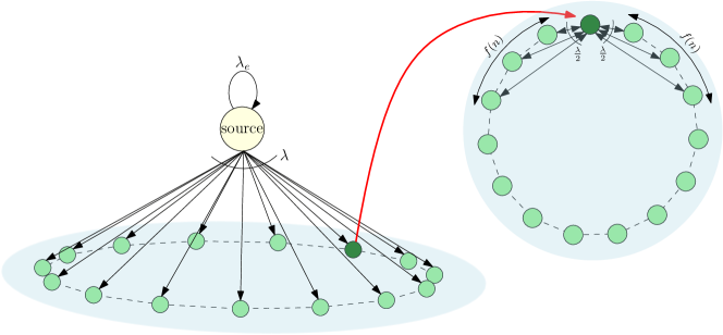
In this work, we consider a general network arranged in the form of a ring, see Fig. 1. The number of neighbors each node has is a positive non-decreasing sub-linear function of , the number of nodes in the network. Each node gossips with neighbors on each side, thus, communicating with neighbors in total. We find a general upper bound on the version age of a single node in such a network. We recover the results obtained for the fully-connected network and the ring network in [10] and [13], by choosing and , respectively, in our result. We analyze how the version age varies as the function grows from to , and find the upper bound for some special cases, such as functions of the form for .
II System Model
We consider a system where we have a source node generating or observing updates as a rate Poisson process independent of all other processes in the network. The source node disseminates these updates to nodes in a network. The network of nodes is denoted by , and hereafter referred to as the ring network. The nodes are placed in a ring formation as shown in Fig. 1. These nodes receive updates from the source node as a combined rate Poisson process, which can be thought of as a thinned process where each node is being updated by the source node as a rate Poisson process.
Each node in the ring network gossips with its neighbors, which are the nearest nodes, i.e., each node gossips with nodes on each side. Each node sends its version of the update to each neighboring node as a rate Poisson process, resulting in a total gossiping rate of per node.
In order to quantify the freshness of version updates, we use the version age metric. First, we define the counting processes associated with the version updates. Let be a counting process associated with the version updates at the source node, i.e., it increases by each time the source gets a new version update. In a similar way, we define the version update of node in the gossip network as the counting process , which maintains the latest version at node . Next, we define the version age of node as , which quantifies the number of versions node is behind compared to the source node. We define the version age of the source node to be , since it always has the latest update. Next, we define the version age of a connected subset of the network as . Finally, we define the limiting average version age of this set as .
The evolution of version age of a particular node in the ring network is as follows: If node in the ring network receives an update directly from the source node, then its version age drops to , since it now has the latest version of the update. If the source node generates or observes a new version of the update, then the version age of node increases by 1. If a neighboring node shares its version of the update, then node keeps the new version if it is fresher than the version it has, otherwise it rejects the update and keeps its own version.
We define the rate of information flow from node to neighboring node as . This is the rate of the Poisson process associated with the updates that node sends to node . We say that node is a neighboring node of set if for some , and define the set of neighboring nodes of as . Next, we define the rate of information flow from node into connected set as and if . Similarly, we define the rate of information flow from the source to set as . We call an edge emanating from node to node an incoming edge into if . We call the set of all incoming edges into set as .
III Version Age of a Single Node
In this section, we calculate an upper bound for the version age of a single node in the generalized ring network, denoted by . We note that the average version age of each node in the network will be the same due to the symmetry in the network. In order to calculate the upper bound, we modify the recursive equations of [10], following the method described in [20].
Lemma 1
For any connected subset of the generalized ring network, we have,
| (1) |
Proof: First, we write the recursive equations from [10],
| (2) |
In order to find an upper bound, we rearrange (2) as,
| (3) |
Now, we define a function which represents the number of incoming edges to set that emanate at node : , where and is the indicator function. Then, we partition into sets according to the number of incoming nodes into from any as,
| (4) |
where . Now, we rewrite (3) as,
| (5) | ||||
| (6) | ||||
| (7) | ||||
| (8) | ||||
| (9) | ||||
| (10) |
where is the total number of incoming edges into set . Rearranging (10) together with the substitution proves the lemma.
Next, we develop a further upper bound for (1) in Lemma 1 by further lower bounding (10). For that, we need to identify a lower bound for in (10) for a fixed number of nodes in on a generalized ring. We have the following lemma.
Lemma 2
On a generalized ring, given all connected subsets such that , the set which has the minimum number of incoming edges is the contiguous set of nodes.
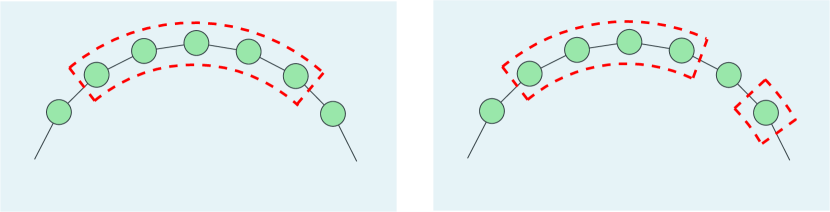
Proof: We denote edges that start at a node in and end at a node in as inner edges. We note that each edge can only be an inner edge or an incoming edge. Hence, the sum of the number of incoming edges and twice the number of inner edges is constant and equal to . Thus, showing that the set of contiguous nodes has the minimum number of incoming edges is the same as showing that it has the maximum number of inner edges. In this proof, we will show that the number of inner edges is the highest. Fig. 2 shows examples of contiguous and non-contiguous sets.
Let the set of contiguous nodes be , and choose any other connected set of nodes and call it . Next, label each node in both sets as and , respectively. The labels start at the node at one end of the set and end at the other end, covering each node in order of their position. Now, we compare each and . We know that both nodes have a total of neighbors.
First, we consider the case where . In this case, has all the other nodes in as a neighbor. Hence, it has inner edges associated with it, and this is the highest achievable. may not have all nodes in as neighbors, and hence has at most the same number of inner edges as . This is true for each consequent node. Hence, adding the number of inner edges of each node in both sets, we see in this case that has more inner edges than .
Next, we consider the case where . Suppose the number of nodes in the set is , then for , shares an inner edge with nodes on one side and neighbors on the other side, which is the highest possible for its position. If , shares an inner edge with nodes on one side and neighbors on the other side, which is the highest possible for its position. If , then all nodes in the set share an inner edge with , which again is the highest possible number. Hence, adding the number of inner edges of each node in both sets, we see in this case that has more inner edges than .
Next, we consider the case where . If , then all neighbors on one side share an inner edge with , and all neighbors on the other side also share an inner edge with , which leads to having the highest possible number of inner edges as it shares an inner edge with all possible nodes in its position. Hence, cannot have more inner edges than . Due to symmetry, this is also true for . Also, if , then all neighbors of share an inner edge with it. Once again, has at most the same number of inner edges. Hence, in this case, adding up the number of inner edges in order for both sets, we conclude that has more inner edges than .
Finally, if , then has the same number of inner edges as . Hence, following the first and second cases above, the contiguous set has the most inner edges.
From the above four cases, we conclude that the set of contiguous nodes has the highest number of inner edges, and hence, the lowest number of incoming edges.
Now, we state and prove our main theorem.
Theorem 1
The version age of a single node in the generalized ring network scales as,
| (11) |
Proof: First, using Lemma 2, we write the exact lower bounds for incoming edges by counting the number of incoming edges of the sets of contiguous nodes. We have three formulae, corresponding to three regions, as follows:
-
1.
:
-
2.
:
-
3.
:
We obtain the first bound by counting the number of inner edges for each node, which is , and then subtracting it from the total number of neighbors . Then, the number of incoming edges for each node is . Since there are nodes in total, the number of incoming edges into set is given by . We carry out a similar calculation to count the number of edges in the third case. In the second case, we simply calculate the number of incoming edges. The nearest neighbors on each side has incoming edges, the second nearest neighbor has incoming edges, and so on. Hence, the total number of incoming edges is given by .
Next, we calculate the sum of recursive terms for each range. Let the sums of the recursive terms for the ranges be , and , respectively.
III-A Range 1
The upper bound for the recursion for is,
| (12) | ||||
| (13) | ||||
| (14) | ||||
| (15) | ||||
| (16) | ||||
| (17) |
where is the Euler-Mascheroni constant.
III-B Range 2
The upper bound for the recursion for is,
| (18) |
where
| (19) | ||||
| (20) | ||||
| (21) |
Substituting this in (18), we get,
| (22) | ||||
| (23) | ||||
| (24) |
Next, we take a logarithm of the th product term in the sum of products term for small enough and use ,
| (25) | ||||
| (26) | ||||
| (27) |
In a similar way, we have,
| (28) |
Substituting (27) and (28) into (24), we obtain,
| (29) | ||||
| (30) |
Now, if , then , and if , then , where is a constant. Next, we convert the Riemann sum associated with the summation term in (30) into a definite integral, and find its exact value. In order to do so, we use step size ,
| (31) |
as and , and the step size tending to . On the other hand, if , then the above integral has lower limit and upper limit a constant, thus giving,
| (32) |
where is a constant. Using this, we obtain,
| (33) | ||||
| (34) |
when , and,
| (35) |
when . Substituting it back in (30), we get,
| (36) | ||||
| (37) |
III-C Range 3
Following a similar calculation to the calculation of ,
| (38) | ||||
| (39) | ||||
| (40) | ||||
| (41) |
where we go from (38) to (39) by approximating the product in the first line of (38) following the calculation of in Range 2. We drop the product in the second line since it is smaller than , and do the regular upper bound in the third line.
Finally, summing the final terms in the three ranges, i.e., in (17), (37), (41), we obtain the upper bound for the age as,
| (42) | ||||
| (43) |
giving the desired result.
| 0.1 | 0.2 | 0.3 | 0.4 | 0.5 | 0.6 | 0.7 | 0.8 | 0.9 | |
|---|---|---|---|---|---|---|---|---|---|
| age scaling | |||||||||
IV Special Cases
IV-A Fully-Connected Network
IV-B Ring With a Fixed Number of Neighbors
Suppose each node in the ring network has neighbors, where is a constant, i.e., . Then, we have,
| (45) |
Hence, in this case, . The bi-directional ring falls under this category with , and we recover [13].
IV-C Ring With a Rational Number of Neighbors,
Here, , with . This case covers functions over a vast range between and . The version age in this case scales as a rational function,
| (46) |
Hence, in this case, .
IV-D Ring With Neighbors
From [10], we know that for a fully-connected network, the version age scales as . Since the networks with considered in this subsection have smaller number of connections, the version age of a single node in these networks is larger. Hence, a lower bound for the version age is . From (11), the upper bound is also . Hence, in this case, the version age of a single node scales as .
V Observations and Remarks
Remark 1
Remark 2
In [20], it was shown that a two dimensional grid has version age scaling of . Each node in the grid network has neighbors. However, in order to achieve a version age scaling of in the generalized ring network, we need , i.e., we need neighbors. One way to explain this difference in the requirement for connectivity to achieve the same version age scaling is the following: According to [20, Remark 5], we can view the grid as a ring network with connections which are not local in nature. Hence, although the number of connections in a grid network is far less compared to the generalized ring network, the version age scaling is the same. This shows us that the geometry of a network can affect the version age significantly, and having few connections between nodes far away is better than having relatively dense connections which are local.
Remark 3
We say that function dominates for a specific value of if . We consider rational functions . We want to see the values of for which the term dominates the term in the upper bound in (43). In (43), we saw that there are two terms in the upper bound: and . In Section IV-C, we consider the version age scaling for , and find that the scaling is as . However, as increases, the rational function grows increasingly slowly and dominates the term only at very high values of . We summarize these numbers in Table I. We note that up to these values of , the version age is upper bounded by , and hence we can consider any to have logarithmic scaling in version age for all practical purposes.
VI Numerical Results
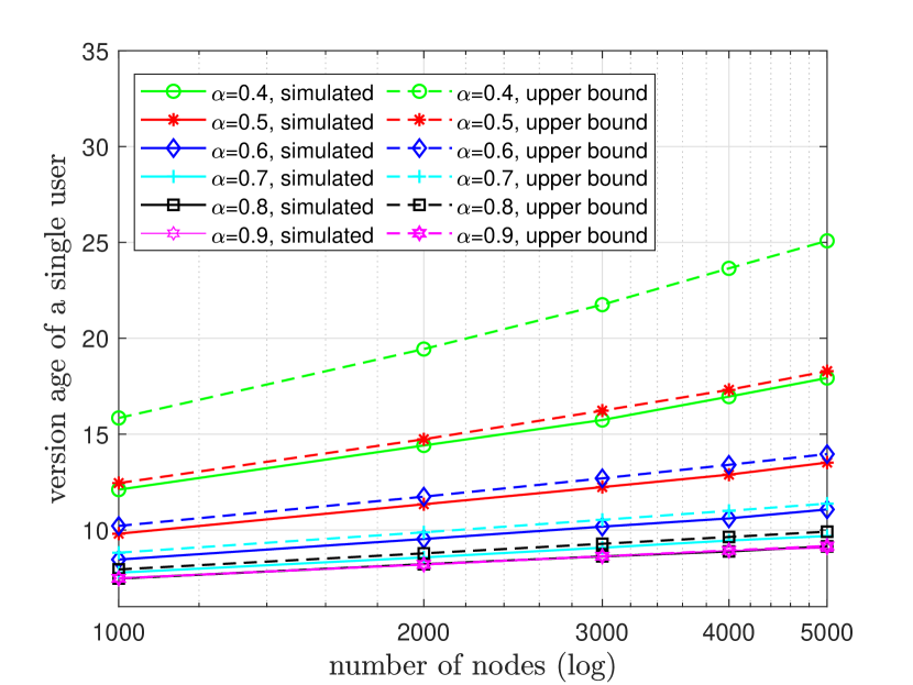
We have seen in Section III, that the upper bound for version age of the generalized ring network depends on the number of nodes , number of connections , and the information flow rates and . We choose in this section.
We plot the variation of the version age for for to . The number of nodes varies from to . Fig. 3 shows that the version age decreases as increases, which is consistent with our theoretical upper bound result. We also observe that the version age plots in Fig. 3 are straight lines, showing that they have approximate scaling for low values of , consistent with Remark 3.
We have not simulated between and , because the function grows slowly. Hence, for small values of , which we are able to run simulations on a PC, the value of might be constant, even if the number of nodes increases. For to , instead of running actual system simulations, we have calculated the upper bound that we obtain from the recursive equations in (12), (18) and (38), and compared it to the upper bound obtained in (43) for , , , , , and observed that the bound gets tight as increases.
VII Conclusion
We considered a gossiping network arranged in a ring. Each node in the network communicates with nodes on each side, sending and receiving updates. We studied the effect of on the version age of a node in the network. We found a general upper bound for the version age of a node that depends only on the number of nodes in the network and . We evaluated the upper bound for several different regimes.
References
- [1] P. Popovski, F. Chiariotti, K. Huang, A. E. Kalør, M. Kountouris, N. Pappas, and B. Soret. A perspective on time toward wireless 6G. Proceedings of the IEEE, 110(8):1116–1146, August 2022.
- [2] S. Kaul, R. D. Yates, and M. Gruteser. Real-time status: How often should one update? In IEEE Infocom, March 2012.
- [3] Y. Sun, I. Kadota, R. Talak, and E. Modiano. Age of information: A new metric for information freshness. Synthesis Lectures on Communication Networks, 12(2):1–224, December 2019.
- [4] R. D. Yates, Y. Sun, D. Brown, S. K. Kaul, E. Modiano, and S. Ulukus. Age of information: An introduction and survey. IEEE Jour. on Selected Areas in Communications, 39(5):1183–1210, May 2020.
- [5] R. D. Yates and S. K. Kaul. The age of information: Real-time status updating by multiple sources. IEEE Transactions on Information Theory, 65(3):1807–1827, March 2018.
- [6] S. Banerjee, S. Ulukus, and A. Ephremides. To re-transmit or not to re-transmit for freshness. May 2023. Available online at arXiv:2305.10392.
- [7] A. Maatouk, S. Kriouile, M. Assaad, and A. Ephremides. The age of incorrect information: A new performance metric for status updates. IEEE/ACM Trans. on Networking, 28(5):2215–2228, October 2020.
- [8] J. Zhong, R. D. Yates, and E. Soljanin. Two freshness metrics for local cache refresh. In IEEE ISIT, June 2018.
- [9] J. Cho and H. Garcia-Molina. Effective page refresh policies for web crawlers. ACM Trans. Database Syst., 28(4):390–426, December 2003.
- [10] R. D. Yates. The age of gossip in networks. In IEEE ISIT, July 2021.
- [11] B. Abolhassani, J. Tadrous, A. Eryilmaz, and E. Yeh. Fresh caching for dynamic content. In IEEE Infocom, May 2021.
- [12] M. Bastopcu and S. Ulukus. Who should Google Scholar update more often? In IEEE Infocom, July 2020.
- [13] B. Buyukates, M. Bastopcu, and S. Ulukus. Version age of information in clustered gossip networks. IEEE Jour. on Selected Areas in Information Theory, 3(1):85–97, March 2022.
- [14] P. Kaswan and S. Ulukus. Susceptibility of age of gossip to timestomping. In IEEE ITW, November 2022.
- [15] P. Kaswan and S. Ulukus. Age of gossip in ring networks in the presence of jamming attacks. In Asilomar Conference, October 2022.
- [16] P. Kaswan and S. Ulukus. Age of information with non-Poisson updates in cache-updating networks. In IEEE ISIT, June 2023.
- [17] P. Mitra and S. Ulukus. ASUMAN: Age sense updating multiple access in networks. In Allerton Conference, September 2022.
- [18] P. Mitra and S. Ulukus. Timely opportunistic gossiping in dense networks. In IEEE Infocom, May 2023.
- [19] M. A. Abd-Elmagid and H. S Dhillon. Distribution of the age of gossip in networks. Entropy, 25(2):364–395, January 2023.
- [20] A. Srivastava and S. Ulukus. Age of gossip on a grid. In Allerton Conference, September 2023. Also available online at arXiv:2307.08670.
- [21] F. Harary and H. Harborth. Extremal animals. Journal of Combinatorics, Information and System Sciences, 1(1):1–8, January 1976.