Absorbing boundary conditions for the Helmholtz equation using Gauss-Legendre quadrature reduced integrations

Abstract.

We introduce a new class of absorbing boundary conditions (ABCs) for the Helmholtz equation. The proposed ABCs can be derived from a certain simple class of perfectly matched layers using $L$ discrete layers and using the $Q_{N}$ Lagrange finite element in conjunction with the $N$-point Gauss-Legendre quadrature reduced integration rule. The proposed ABCs are classified by a tuple $(L,N)$, and achieve reflection error of order $O(R^{2LN})$ for some $R<1$. The new ABCs generalise the perfectly matched discrete layers proposed by Guddati and Lim [Int. J. Numer. Meth. Engng 66 (6) (2006) 949-977], including them as type $(L,1)$. An analysis of the proposed ABCs is performed motivated by the work of Ainsworth [J. Comput. Phys. 198 (1) (2004) 106-130]. The new ABCs facilitate numerical implementations of the Helmholtz problem with ABCs if $Q_{N}$ finite elements are used in the physical domain. Moreover, giving more insight, the analysis presented in this work potentially aids with developing ABCs in related areas.

1. Introduction

The Helmholtz equation is of interest in many fields in physics and engineering. We are particularly interested in solving the Helmholtz equation in unbounded domains. As the standard numerical methods such as finite element methods require finite computational domains, solving such problem numerically requires one to map the original problem in an unbounded domain to one in a bounded domain. This is commonly achieved by truncating the unbounded domain and applying an artificial boundary condition representing the original unboundedness on or in the vicinity of the surface of truncation. Such artificial boundary conditions are called absorbing boundary conditions (ABCs). The accuracy of an ABC is often measured by the reflection coefficient, the ratio of the spurious incoming wave to the outgoing wave. Many ABCs have been proposed in the last decades. Among them, the complete radiation boundary conditions (CRBCs) and the perfectly matched discrete layers (PMDLs) are known to be especially accuate and efficient.

ABCs have typically been studied for the wave equation, from which those for the Helmholtz equation can readily be derived. The early ABCs proposed and studied in [17, 18, 12, 27, 28] involved high-order temporal and spatial derivatives on the artificial boundary. The Higdon ABCs [27] were designed to annihilate $L$ purely propagating plane waves and included $L$-th order temporal and normal derivatives of the solution on the boundary. The Givoli-Neta ABCs [19] introduced auxiliary functions on the boundary and recast the classic Higdon ABCs as systems of $L$ equations that only involved first-order temporal and normal derivatives, greatly facilitating the numerical implementations. Hagstrom-Warburton ABCs [24] symmetrised the Givoli-Neta ABCs, squaring the reflection coefficients. The CRBCs [25] further improved the behaviour by directly taking into account the waves that decays while propagating. The significance of treating such wave mode was also noted in [28]. This class of ABCs are generally known to show exellent performances regardless of the choice of the parameters. Since it was demanded that the auxiliary functions were only defined on the boundary, the above classes of ABCs required reformulations to remove the unfavorable first-order normal derivatives. In [19] the Givoli-Neta ABCs were rewritten in forms that only involved up to second-order temporal and tangential derivatives; such formulations are thus called second-order formulations. The second-order formulations of the later ABCs were derived in [24, 31]. Further, in multidimensions, the above classes of ABCs required special treatment on edges and corners on which multiple faces met. The edge/corner compatibility conditions were derived for the Hagstrom-Warburton ABCs in [24] and for the later ABCs in [31]. The second-order formulations as well as the edge/corner compatibility conditions require one to work with complex systems of PDEs on the artificial boundary that are distinct from the wave equation or the Helmholtz equation solved in the physical domain. As noted shortly, the PMDLs have a clear advantage in this regard when the Helmholtz equation is considered. Having been developed for the wave equation, however, the CRBCs and the other related ABCs typically handle the wave equation more directly and efficiently. As we focus on the Helmholtz equation in this work, we leave further discussion in this regard for future work.

The perfectly matched layers (PMLs) formulation is another class of conditions widely used to approximate the effect of the original unboundedness. The PMLs were originally proposed in [13] for the time-domain electromagnetics, in which artificial damping terms were added in the vicinity of the domain of interest, or the physical domain. We call the domain in which damping terms were added the artificial domain, and call the union of the physical domain and the artifical domain the computational domain. The addition of the artificial damping was later reinterpreted as a complex coordinate transformation in the frequency-domain in [16]. As for the Helmholtz equation, the PMLs have been more popular than the CRBCs and the other related ABCs, presumably because, a single PDE, which reduces to the standard Helmholtz equation for a particular choice of parameters, monolithically governs the entire computational domain even in existence of edges and corners, which facilitates numerical implementations; see, e.g., [13] for the initail treatment of the corners. Despite the popularity of the PMLs, however, the accuracy of the PMLs are known to be sensitive to the choice of the parameters, which are hard to tune a priori, and the ABCs often outperform the PMLs in terms of accuracy. An attempt to optimise the performance of the PMLs for a particular finite difference scheme [7] then inspired the development of the PMDLs [21, 23], which was designed for finite element methods. The PMDLs formulation is effectively obtained by first writing the PMLs formulation in the weak form, then using the linear finite element approximation with midpoint reduced integration in the artificial domain in the direction normal to the artificial boundary. It has been shown that the PMDLs are essentially equivalent to the CRBCs, but the PMDLs being based on the PMLs, they inherit the favourable property of the PMLs, and allow one to work with a single equation similar to the standard Helmholtz equation across the computational domain even if edges and corners exist. Specifically, if the $Q_{1}$ tensor-product Lagrange finite elements are used in the physical domain, that Helmholtz-like equation can be discretised monolithically using the $Q_{1}$ elements on the entire computational domain, and one only needs to use different quadrature rules in the physical and artificial domains. If $Q_{N}$ elements with $N>1$ are used in the physical domain, one needs to handle the artifical domain separately as the PMDLs require linear approximation in the artificial domain in the direction normal to the boundary. Even in such cases, however, the PMDLs are generally more tractable than the CRBCs.

In this work we propose a new class of ABCs for the Helmholtz equation that generalises the PMDLs. The proposed ABCs are derived from a certain simple class of perfectly matched layers with $L$ discrete layers in the artificial domain, using the $Q_{N}$ tensor-product Lagrange finite elements in conjunction with the $N$-point Gauss-Legendre quadrature reduced integration in the artificial domain. Thus, the proposed ABCs can be classified by a tuple $(L,N)$, with the PMDLs represented by $(L,1)$. The ABCs of type $(L,N)$ and those of type $(LN,1)$ introduce the same number of auxiliary degrees of freedom in the artificial domain, and they are as accurate as each other. Like the PMDLs, the proposed ABCs only involve a single Helmholtz-like equation over the entire computational domain even if edges and corner exist, but they further allow for monolithic discretisations over the computational domain even when the $Q_{N}$ finite elements with $N>1$ are used in the physical domain. Furthermore, we present an analysis of the proposed ABCs, strongly motivated by the techniques used in [2], in which dispersive and dissipative behaviour of high-order discontinuous Galerkin methods were studied, and in the related works [1, 4, 3], that is to give more insight into the problem.

In Sec. 2 and Sec. 3 we introduce the Helmholtz equation and the standard PMLs formulation. In Sec. 4 we study a certain simple PMLs formulation in detail, which will aid us with developing the new ABCs. In Sec. 5 we introduce the discretised weak forms of the PMLs formulations introduced in Sec. 3 and Sec. 4. In Sec. 6 we introduce and study the new class of ABCs. In Sec. 7 we show one- and three-dimensional examples. In Sec. 8 we summarise this work and discuss future works.

2. The Helmholtz equation

The Helmholtz equation in ^d, $d\in\mathbb{N}$, to be solved for $u(x_{1},x_{2},\cdots,x_{d})$ is given by:

$$s^{2}u-u_{,ii} =f\quad\textrm{in }^{d},$$ (1)

where sum is taken over $i\in\{1,\cdots,d\}$, $s\in\mathbb{C}$ is a complex number with $\text{Re}(s)\geq 0$, and $f$ is a spatial function that is assumed to have a compact support in $x<-\delta$ for some $\delta>0$, where $x:=x_{1}$ is the first coordinate variable. Provided that the domain of interest is $x<0$, we are going to work with:

$$s^{2}u-u_{,ii} =0\quad\textrm{in }x>-\delta.$$ (2)

Taking the Fourier transform of (2) in all the coordinate variables except $x:=x_{1}$, we obtain an ordinary differential equation to be solved for, with an abuse of notation, $u(x)$ as:

$$\gamma^{2}u-u_{,xx}=0\quad\textrm{in }x>-\delta,$$ (3)

where $\gamma:=\sqrt{s^{2}+k^{2}}$, where $k:=\sqrt{k_{i}k_{i}}$ (sum on $i\in\{2,\cdots,d\}$), where $k_{i}\in$ is the dual variable of $x_{i}$. If (1) is derived by taking the Laplace transform in time of the wave equation as in [25], we have $\text{Re}(s)>0$, in which case we consider a Riemann surface with branch cut on $(-\mathfrak{i}\infty,-\mathfrak{i}k)\cup(+\mathfrak{i}k,+\mathfrak{i}\infty)$ and choose the branch of $\sqrt{s^{2}+k^{2}}$ so that $\gamma=+k$ when $s=0$. In this case we have $\text{Re}(\gamma)>0$. If (1) is derived from the time-harmonic assumption of the wave equation, we have $s=\mathfrak{i}\omega$, $\omega\in$, and we define the value of $\gamma$ as the limit in the above branch along $s=\mathfrak{i}\omega+\epsilon$ as $\epsilon\rightarrow 0^{+}$. The following two properties then hold for $\text{Re}(s)\geq 0$:

$$[\text{Im}(\gamma)\!\cdot\!\text{Im}(s)>0\textrm{ and }\text{Re}(\gamma)\geq 0]\text{ or }[\text{Im}(\gamma)=0\textrm{ and }\text{Re}(\gamma)>0],$$ (4a)

$$\textrm{Re}\left(\frac{\gamma}{a\!\cdot\!s+b}\right)>0,\quad\forall a,b>0,$$ (4b)

unless $s=\pm\mathfrak{i}k$, which is not of interest.

One can readily solve (3) up to two undertermind coefficients, $c_{-}$ and $c_{+}$, as:

$$u(x)=c_{-}e^{+\gamma x}+c_{+}e^{-\gamma x}.$$ (5)

Noting (4a), one can see that $e^{+\gamma x}$ represents the wave that is incoming and/or grows as $x\rightarrow+\infty$ and $e^{-\gamma x}$ represents the wave that is outgoing and/or decays as $x\rightarrow+\infty$. We require $c_{-}=0$, or:

$$\frac{c_{-}}{c_{+}}=0,$$ (6)

only leaving the outgoing/decaying wave. This ratio in (6) is called the reflection coefficient, and is an important measure of the accuracy of absorbing boundary conditions (ABCs). The outgoing/decaying wave solution also satisfies:

$$u_{,x}(0)+\gamma u(0)=0,$$ (7)

which is known as the Sommerfeld radiation condition (at $x=0$). The extent to which a given ABC approximates (7) gives another important measure of the accuracy of that condition.

Our domain of interest, or the physical domain, being $x<0$, we are to truncate the right half-domain. Although (7) gives the exact boundary condition for the outgoing/decaying wave at $x=0$ for the one-dimensional problem (3) for a given $k\in$, its multidimensional counterpart that is exact for all $k$ does not exist. In the followng sections we work with several conditions applied in the vicinity of $x=0$ outside the physical domain, which we call the artificial domain, that are to approximate the effect of the unboundedness of $x>0$, ideally only admitting the outgoing/decaying wave at $x=0$.

3. Perfectly matched layers

The perfectly matched layers (PMLs) method was originally developed for the time-domain electromagnetics in [13] by adding artificial damping terms in the artificial domain so that the outgoing wave attenuates. The addition of artificial damping was later reinterpreted as complex coordinate transformation in [16]. In this section we briefly introduce the PMLs formulation using the idea of complex coordinate transformation. Although the PMLs formulation is conventionally derived for a simplified version of (3), which one can obtain by setting $s=\mathfrak{i}\omega$ and $k=0$, or $\gamma=\mathfrak{i}\omega$, we here use (3) directly to take into account the effect of multidimensions.

The crucial step in deriving the PMLs formulation is to introduce a complex coordinate transformation, $\tilde{\chi}:\rightarrow\mathbb{C}$, which is sufficiently smooth and satisfies $\tilde{\chi}(x)=x$ in $x<0$. We denote the transformed coordinate by $\tilde{x}:=\tilde{\chi}(x)$, and consider solving the following modified version of (3) for $\tilde{u}(\tilde{x})$:

$$\gamma^{2}\tilde{u}-\tilde{u}_{,\tilde{x}\tilde{x}}=0\quad x>-\delta.$$ (8)

Defining $u^{\dagger}:=\tilde{u}\circ\tilde{\chi}$, one can rewrite (8) in terms of $x$ as a problem to be solved for $u^{\dagger}(x)$ as:

$$\frac{\gamma^{2}}{g^{\textrm{PML}}}u^{\dagger}-(g^{\textrm{PML}}u^{\dagger}_{,x})_{,x} =0\quad x>-\delta,$$ (9)

where:

$$g^{\textrm{PML}}(x):=\frac{\thinspace\mathrm{d}x}{\thinspace\mathrm{d}\tilde{x}},$$ (10)

where the superscript $(\cdot)^{\textrm{PML}}$ is used to represent PMLs. Note that $g^{\textrm{PML}}(x)=1$ in $x<0$, so (9) reduces to the standard Helmholtz equation (3) in $x<0$. By construction, the solution to (9) is readily obtained as:

$$u^{\dagger}(x)=c^{\dagger}_{-}e^{+\gamma\tilde{\chi}(x)}+c^{\dagger}_{+}e^{-\gamma\tilde{\chi}(x)}.$$ (11)

The complex transformation function $\tilde{\chi}(x)$ is chosen so that the outgoing/decaying wave, represented by $\exp{(-\gamma\tilde{\chi}(x))}$, attenuates as $x\rightarrow+\infty$. A popular choice in the common setting of $\gamma=\mathfrak{i}\omega$ is $\tilde{\chi}(x)=x+(\omega_{0}/\mathfrak{i}\omega)\!\cdot\!\int_{-\infty}^{x}f^{\textrm{pml}}(\tau)\thinspace\mathrm{d}\tau$, where $\omega_{0}$ is a positive constant for non-dimensionalisation and $f^{\textrm{pml}}(x)=0$ in $x\leq 0$ and $f^{\textrm{pml}}(x)>0$ in $x>0$. The outgoing wave solution then becomes $\exp{(-\gamma x)}\!\cdot\!\exp{(-\omega_{0}\int_{-\infty}^{x}f^{\textrm{pml}}(\tau)\thinspace\mathrm{d}\tau)}$, which coincides with the exact outgoing wave solution $\exp{(-\gamma x)}$ in $x<0$ and decays exponentially as $x\rightarrow+\infty$. For convenience, we here introduce a set of grid points, $\{x_{-1,x_{0},\cdots,x_{L}}\}$, where $-\delta<x_{-1}<x_{0}=0<x_{1}<\cdots<x_{L}$. The above observation justifies one in truncating the right half-space $x>x_{L}$ for $x_{L}$ sufficiently large such that $u^{\dagger}(x_{L})\approx 0$. We thus obtain the PMLs formulation to be solved for $u^{\textrm{PML}}(x)$ up to one undetermined coefficient as:

$$\frac{\gamma^{2}}{g^{\textrm{PML}}}u^{\textrm{PML}}-(g^{\textrm{PML}}u^{\textrm{PML}}_{,x})_{,x} =0\quad\textrm{ in }x_{-1}<x<x_{L},$$ (12a)

$$u^{\textrm{PML}}(x_{L}) =0,$$ (12b)

(12b) is called the termination condition. (12a) can readily be solved up to two undetermined coefficients, $c^{\textrm{PML}}_{-}$ and $c^{\textrm{PML}}_{+}$, as:

$$u^{\textrm{PML}}(x)=c^{\textrm{PML}}_{-}e^{+\gamma\tilde{\chi}(x)}+c^{\textrm{PML}}_{+}e^{-\gamma\tilde{\chi}(x)}.$$ (13)

Applying (12b), one can solve (12) up to one undertermined coefficient as desired. The reflection coefficient of the solution thus obtained is given as:

$$\frac{c^{\textrm{PML}}_{-}}{c^{\textrm{PML}}_{+}}=-\left(e^{-\gamma\tilde{\chi}(x_{L})}\right)^{2}.$$ (14)

The solution satisfies the following approximate Sommerfeld radiation condition:

$$u^{\textrm{PML}}_{,x}(0)+\gamma\left(\frac{1+\left(e^{-\gamma\tilde{\chi}(x_{L})}\right)^{2}}{1-\left(e^{-\gamma\tilde{\chi}(x_{L})}\right)^{2}}\right)u^{\textrm{PML}}(0)=0.$$ (15)

In the spatially continuous setting $\exp{(-\gamma\tilde{\chi}(x_{L}))}^{2}$ can be made as small as desired by manipulating $\tilde{\chi}(x)$, and the reflection coefficient (14) and the approximate Sommerfeld radiation condition (15) can be made arbitrarily close to the exact expressions (6) and (7). As mentioned in Sec. 5, this will no longer be the case after discretisation. Finally, we note that, if $g^{\textrm{PML}}(x_{L})u^{\textrm{PML}}_{,x}(x_{L})+\gamma u^{\textrm{PML}}(x_{L})=0$, which we call the transformed Sommerfeld radiation condition, was applied at $x=x_{L}$ in place of the termination condition (12b), we would obtain $c^{\textrm{PML}}_{-}=0$ and $u^{\textrm{PML}}(x)$ would represent the exact outgoing/decaying wave solution in $x<0$ despite the existence of the PMLs.

4. Layerwise constant perfectly matched layers

Before introducing the new ABCs, it is instructive to study the layerwise constant perfectly matched layers. We first define a layerwise constant complex function, $g^{\textrm{LWC}}(x)$, as:

$$g^{\textrm{LWC}}(x):=\gamma_{l}\quad\textrm{ in }x_{l-1}<x\leq x_{l},\quad l\in\{0,\cdots,L\},$$ (16)

where $\gamma_{l}\in\mathbb{C}$ is a complex constant and the superscript $(\cdot)^{\textrm{LWC}}$ is used to represent layerwise constant PMLs. $\gamma_{0}$ is defined to be $1$, and $\gamma_{l}$, $l\in\{1,\cdots,L\}$, is chosen so that $\text{Re}(\gamma/\gamma_{l})>0$; this is achieved by letting $\gamma_{l}=a\cdot s+b$ for some $a,b>0$, according to Property (4b).

We solve a problem that is similar to (12), but explicitly handling the discontinuities of $g^{\textrm{LWC}}(x)$. Specifically, we define $u^{\textrm{LWC}}(x)$ as:

$$u^{\textrm{LWC}}(x):=u^{\textrm{LWC}}_{l}(x)\quad\textrm{ on }[x_{l-1},x_{l}],\quad l\in\{0,\cdots,L\},$$ (17)

and solve the following system of equations for $u^{\textrm{LWC}}_{l}(x)$, $l\in\{0,\cdots,L\}$, which is assumed to be sufficiently smooth in $(x_{l-1}-\epsilon,x_{l}+\epsilon)$ for some $\epsilon>0$:

$$\frac{\gamma^{2}}{\gamma_{l}}u^{\textrm{LWC}}_{l}-(\gamma_{l}u^{\textrm{LWC}}_{l,x})_{,x} =0\quad\textrm{ in }(x_{l-1},x_{l}), \forall l\in\{0,\cdots,L\},$$ (18a)

$$\gamma_{l}u^{\textrm{LWC}}_{l,x}(x_{l})-\gamma_{l+1}u^{\textrm{LWC}}_{l+1,x}(x_{l}) =0, \forall l\in\{0,\cdots,L-1\},$$ (18b)

$$u^{\textrm{LWC}}_{l}(x_{l})-u^{\textrm{LWC}}_{l+1}(x_{l}) =0, \forall l\in\{0,\cdots,L-1\},$$ (18c)

$$u^{\textrm{LWC}}_{L}(x_{L}) =0.$$ (18d)

Once we solve (18a) up to two undetermined coefficients for each $l$, we will be left with a system of $L+L+1=2(L+1)-1$ equations for $2(L+1)$ unknowns.

4.1. Domain equations

One can readily solve (18a) for $u^{\textrm{LWC}}_{l}(x)$ for each $l\in\{0,\cdots,L\}$ up to two undertermined coefficients, $c^{\textrm{LWC}}_{l,\textrm{even}}$ and $c^{\textrm{LWC}}_{l,\textrm{odd}}$, as:

$$u^{\textrm{LWC}}_{l}(x)=c^{\textrm{LWC}}_{l,\textrm{even}}\!\cdot\!\left(\frac{e^{+\frac{\gamma}{\gamma_{l}}\bigl{(}x-x_{l-\frac{1}{2}}\bigr{)}}+e^{-\frac{\gamma}{\gamma_{l}}\bigl{(}x-x_{l-\frac{1}{2}}\bigr{)}}}{2}\right)+c^{\textrm{LWC}}_{l,\textrm{odd}}\!\cdot\!\left(\frac{e^{+\frac{\gamma}{\gamma_{l}}\bigl{(}x-x_{l-\frac{1}{2}}\bigr{)}}-e^{-\frac{\gamma}{\gamma_{l}}\bigl{(}x-x_{l-\frac{1}{2}}\bigr{)}}}{2}\right),$$ (19)

where $x_{l-\frac{1}{2}}=(x_{l-1}+x_{l})/2$. We are now left with $2(L+1)-1$ equations for $2(L+1)$ unknowns.

4.2. Interface conditions

Using (19), (18c) and (18b) can be written as:

$$\begin{pmatrix}S^{\textrm{LWC}}_{\textrm{even}}(\alpha_{l})&S^{\textrm{LWC}}_{\textrm{odd}}(\alpha_{l})\\ S^{\textrm{LWC}}_{\textrm{odd}}(\alpha_{l})&S^{\textrm{LWC}}_{\textrm{even}}(\alpha_{l})\end{pmatrix}\begin{pmatrix}c^{\textrm{LWC}}_{l,\textrm{even}}\\ c^{\textrm{LWC}}_{l,\textrm{odd}}\end{pmatrix}-\begin{pmatrix}\phantom{-}S^{\textrm{LWC}}_{\textrm{even}}(\alpha_{l+1})&-S^{\textrm{LWC}}_{\textrm{odd}}(\alpha_{l+1})\\ -S^{\textrm{LWC}}_{\textrm{odd}}(\alpha_{l+1})&\phantom{-}S^{\textrm{LWC}}_{\textrm{even}}(\alpha_{l+1})\end{pmatrix}\begin{pmatrix}c^{\textrm{LWC}}_{l+1,\textrm{even}}\\ c^{\textrm{LWC}}_{l+1,\textrm{odd}}\end{pmatrix}=\begin{pmatrix}0\\ 0\end{pmatrix},$$ (20)

where $S^{\textrm{LWC}}_{\textrm{even}}(\alpha_{l})$ and $S^{\textrm{LWC}}_{\textrm{odd}}(\alpha_{l})$ are defined as:

$$S^{\textrm{LWC}}_{\textrm{even}}(\alpha_{l}): =\frac{e^{+\frac{\alpha_{l}}{2}}+e^{-\frac{\alpha_{l}}{2}}}{2},$$ (21a)

$$S^{\textrm{LWC}}_{\textrm{odd}}(\alpha_{l}): =\frac{e^{+\frac{\alpha_{l}}{2}}-e^{-\frac{\alpha_{l}}{2}}}{2},$$ (21b)

where:

$$\alpha_{l}:=\frac{\gamma}{\gamma_{l}}h_{l},$$ (22)

where $h_{l}:=x_{l}-x_{l-1}$. Note that $\gamma_{0}=1$ and we chose $\gamma_{l}$, $l\in\{1,\cdots,L\}$, so that $\text{Re}(\alpha_{l})>0$. Performing eigendecompositions of the matrices appering in (20), we have:

$$\begin{pmatrix}S^{\textrm{LWC}}_{\textrm{even}}(\alpha_{l})&S^{\textrm{LWC}}_{\textrm{odd}}(\alpha_{l})\\ S^{\textrm{LWC}}_{\textrm{odd}}(\alpha_{l})&S^{\textrm{LWC}}_{\textrm{even}}(\alpha_{l})\end{pmatrix} =\Phi\begin{pmatrix}e^{+\frac{\alpha_{l}}{2}}&0\\ 0&e^{-\frac{\alpha_{l}}{2}}\end{pmatrix}\Phi^{\textrm{T}},$$ (23a)

$$\begin{pmatrix}\phantom{-}S^{\textrm{LWC}}_{\textrm{even}}(\alpha_{l+1})&-S^{\textrm{LWC}}_{\textrm{odd}}(\alpha_{l+1})\\ -S^{\textrm{LWC}}_{\textrm{odd}}(\alpha_{l+1})&\phantom{-}S^{\textrm{LWC}}_{\textrm{even}}(\alpha_{l+1})\end{pmatrix} =\Phi\begin{pmatrix}e^{-\frac{\alpha_{l+1}}{2}}&0\\ 0&e^{+\frac{\alpha_{l+1}}{2}}\end{pmatrix}\Phi^{\textrm{T}},$$ (23b)

where $\Phi$ is a $2\times 2$ orthonormal matrix of eigenvectors that is independent of the layer parameter $l$:

$$\Phi=\begin{pmatrix}\frac{1}{\sqrt{2}}&\phantom{-}\frac{1}{\sqrt{2}}\\ \frac{1}{\sqrt{2}}&-\frac{1}{\sqrt{2}}\end{pmatrix}.$$ (24)

Using (23) and (24), (20) reduces to:

$$\begin{pmatrix}\frac{e^{+\frac{\alpha_{l}}{2}}}{e^{-\frac{\alpha_{l+1}}{2}}}&0\\ 0&\frac{e^{-\frac{\alpha_{l}}{2}}}{e^{+\frac{\alpha_{l+1}}{2}}}\end{pmatrix}\begin{pmatrix}c^{\textrm{LWC}}_{l,-}\\ c^{\textrm{LWC}}_{l,+}\end{pmatrix}=\begin{pmatrix}c^{\textrm{LWC}}_{l+1,-}\\ c^{\textrm{LWC}}_{l+1,+}\end{pmatrix},$$ (25)

where:

$$\begin{pmatrix}c^{\textrm{LWC}}_{l,-}\\ c^{\textrm{LWC}}_{l,+}\end{pmatrix}=\Phi^{\textrm{T}}\begin{pmatrix}c^{\textrm{LWC}}_{l,\textrm{even}}\\ c^{\textrm{LWC}}_{l,\textrm{odd}}\end{pmatrix}.$$ (26)

Using (25), one can recursively eliminate $c^{\textrm{LWC}}_{l,-}$ and $c^{\textrm{LWC}}_{l,+}$, $l\in\{1,\cdots,L-1\}$, to obtain:

$$\begin{pmatrix}\prod\limits_{l=0}^{L-1}\frac{e^{+\frac{\alpha_{l}}{2}}}{e^{-\frac{\alpha_{l+1}}{2}}}&0\\ 0&\prod\limits_{l=0}^{L-1}\frac{e^{-\frac{\alpha_{l}}{2}}}{e^{+\frac{\alpha_{l+1}}{2}}}\end{pmatrix}\begin{pmatrix}c^{\textrm{LWC}}_{0,-}\\ c^{\textrm{LWC}}_{0,+}\end{pmatrix}=\begin{pmatrix}c^{\textrm{LWC}}_{L,-}\\ c^{\textrm{LWC}}_{L,+}\end{pmatrix}.$$ (27)

We are now left with $1$ equation for $2$ unknowns.

$c^{\textrm{LWC}}_{0,-}$ and $c^{\textrm{LWC}}_{0,+}$ respectively represent the incoming/growing wave and the outgoing/decaying wave. Here, we suppose that there was an additional layer $[x_{-2},x_{-1}]$ with $-\delta<x_{-2}<x_{-1}<0$ and define $h_{-1}:=x_{-1}-x_{-2}=h_{0}$ and $\gamma_{-1}:=1=\gamma_{0}$. If we extended the above analysis to include $[x_{-2},x_{-1}]$, the solution $u_{-1}^{\textrm{LWC}}$ in $(x_{-2}-\epsilon,x_{-1}+\epsilon)$ would be represented in terms of $c^{\textrm{LWC}}_{-1,-}$ and $c^{\textrm{LWC}}_{-1,+}$. Using (25) with $l=-1$ and (22), $c^{\textrm{LWC}}_{-1,-}$ and $c^{\textrm{LWC}}_{-1,+}$ would be related to $c^{\textrm{LWC}}_{0,-}$ and $c^{\textrm{LWC}}_{0,+}$ as:

$$\begin{pmatrix}e^{+\gamma h_{0}}&0\\ 0&e^{-\gamma h_{0}}\end{pmatrix}\begin{pmatrix}c^{\textrm{LWC}}_{-1,-}\\ c^{\textrm{LWC}}_{-1,+}\end{pmatrix}=\begin{pmatrix}c^{\textrm{LWC}}_{0,-}\\ c^{\textrm{LWC}}_{0,+}\end{pmatrix},$$ (28)

which implies the above statement.

4.3. Termination condition

Finally, we apply the termination condition (18d). Using (19) with $l=L$ along with (21), (18d) can be written as:

$$S^{\textrm{LWC}}_{\textrm{even}}(\alpha_{L})\!\cdot\!c^{\textrm{LWC}}_{L,\textrm{even}}+S^{\textrm{LWC}}_{\textrm{odd}}(\alpha_{L})\!\cdot\!c^{\textrm{LWC}}_{L,\textrm{odd}}=0,$$ (29)

or, rewriting in terms of $c^{\textrm{LWC}}_{L,-}$ and $c^{\textrm{LWC}}_{L,+}$ using (26):

$$\frac{1}{\sqrt{2}}\begin{pmatrix}e^{+\frac{\alpha_{L}}{2}}\hskip 5.0pte^{-\frac{\alpha_{L}}{2}}\end{pmatrix}\begin{pmatrix}c^{\textrm{LWC}}_{L,-}\\ c^{\textrm{LWC}}_{L,+}\end{pmatrix}=0.$$ (30)

Using (27) in conjunction with (30), we obtain:

$$\frac{c^{\textrm{LWC}}_{0,-}}{c^{\textrm{LWC}}_{0,+}}=-\left(e^{-\alpha_{0}}\right)\prod_{l=1}^{L}\left(e^{-\alpha_{l}}\right)^{2},$$ (31)

which compares with the reflection coefficient for the standard PMLs formulation (14). Like (14), (31) can be made arbitrarily small by manipulating the values of $\gamma_{l}$, $l\in\{1,\cdots,L\}$. in the spatially continuous setting. The system (18) has now been solved up to one undermined coefficient as desired.

We now study the ability of the layerwise constant PMLs to approximate the Sommerfeld radiation condition (7). For this analysis, (18a) only needs to be satisfied for $l\in\{1,\cdots,L\}$. Following the same line as the the derivation of (31), we have:

$$\frac{c^{\textrm{LWC}}_{1,-}}{c^{\textrm{LWC}}_{1,+}}=-\left(e^{-\alpha_{1}}\right)\prod_{l=2}^{L}\left(e^{-\alpha_{l}}\right)^{2}.$$ (32)

Using (19) with $l=1$ along with (21), (18b) and (18c) with $l=0$, and $\gamma_{0}=1$, we have:

$$u^{\textrm{LWC}}_{0}(0) =S^{\textrm{LWC}}_{\textrm{even}}(\alpha_{1})\!\cdot\!c^{\textrm{LWC}}_{1,\textrm{even}}-S^{\textrm{LWC}}_{\textrm{odd}}(\alpha_{1})\!\cdot\!c^{\textrm{LWC}}_{1,\textrm{odd}},$$ (33a)

$$u^{\textrm{LWC}}_{0,x}(0) =-\gamma\left(S^{\textrm{LWC}}_{\textrm{odd}}(\alpha_{1})\!\cdot\!c^{\textrm{LWC}}_{1,\textrm{even}}-S^{\textrm{LWC}}_{\textrm{even}}(\alpha_{1})\!\cdot\!c^{\textrm{LWC}}_{1,\textrm{odd}}\right)$$ (33b)

or, writing in terms of $c^{\textrm{LWC}}_{1,-}$ and $c^{\textrm{LWC}}_{1,+}$ using (26):

$$u^{\textrm{LWC}}_{0}(0) =\frac{1}{\sqrt{2}}\begin{pmatrix}e^{-\frac{\alpha_{1}}{2}}\hskip 5.0pte^{+\frac{\alpha_{1}}{2}}\end{pmatrix}\begin{pmatrix}c^{\textrm{LWC}}_{1,-}\\ c^{\textrm{LWC}}_{1,+}\end{pmatrix},$$ (34a)

$$u^{\textrm{LWC}}_{0,x}(0) =-\frac{1}{\sqrt{2}}\gamma\begin{pmatrix}-e^{-\frac{\alpha_{1}}{2}}\hskip 5.0pte^{+\frac{\alpha_{1}}{2}}\end{pmatrix}\begin{pmatrix}c^{\textrm{LWC}}_{1,-}\\ c^{\textrm{LWC}}_{1,+}\end{pmatrix}.$$ (34b)

Using (34) in conjunction with (32), we obtain the approximate Sommerfeld radiation condition provided by the layerwise constant PMLs as:

$$u^{\textrm{LWC}}_{0,x}(0)+\gamma\left(\frac{1+\prod\limits_{l=1}^{L}\left(e^{-\alpha_{l}}\right)^{2}}{1-\prod\limits_{l=1}^{L}\left(e^{-\alpha_{l}}\right)^{2}}\right)u^{\textrm{LWC}}_{0}(0)=0,$$ (35)

which compares with (15). Note, in the spatially continuous setting, the approximation (35) can be made arbitrarily accurate by manipulating the values of $\gamma_{l}$, $l\in\{1,\cdots,L\}$.

4.4. Transformed Sommerfeld radiation condition

In this section we consider applying the transformed Sommerfeld radiation condition, $\gamma_{L}u^{\textrm{LWC}}_{L,x}(x_{L})+\gamma u^{\textrm{LWC}}_{L}(x_{L})=0$, at $x=x_{L}$ in stead of the termination condition (18d). Using (19) with $l=L$ along with (21), the transformed Sommerfeld radiation condition can be written as:

$$\gamma\left(S^{\textrm{LWC}}_{\textrm{odd}}(\alpha_{L})\!\cdot\!c^{\textrm{LWC}}_{L,\textrm{even}}+S^{\textrm{LWC}}_{\textrm{even}}(\alpha_{L})\!\cdot\!c^{\textrm{LWC}}_{L,\textrm{odd}}\right)+\gamma\left(S^{\textrm{LWC}}_{\textrm{even}}(\alpha_{L})\!\cdot\!c^{\textrm{LWC}}_{L,\textrm{even}}+S^{\textrm{LWC}}_{\textrm{odd}}(\alpha_{L})\!\cdot\!c^{\textrm{LWC}}_{L,\textrm{odd}}\right)=0.$$ (36)

Simplifying the expression and rewriting in terms of $c^{\textrm{LWC}}_{L,-}$ and $c^{\textrm{LWC}}_{L,+}$ using (26), we have:

$$\sqrt{2}\gamma\begin{pmatrix}e^{+\frac{\alpha_{L}}{2}}\hskip 5.0pt0\end{pmatrix}\begin{pmatrix}c^{\textrm{LWC}}_{L,-}\\ c^{\textrm{LWC}}_{L,+}\end{pmatrix}=0.$$ (37)

Using (27) in conjunction with (37), we obtain:

$$\frac{c^{\textrm{LWC}}_{0,-}}{c^{\textrm{LWC}}_{0,+}}=0,$$ (38)

which implies that the layerwise constant PMLs with the transformed Sommerfeld radiation condition at $x=x_{L}$ only admit the outgoing/decaying wave at $x=0$.

Following the same lines as the derivation of (35), one can show that the layerwise constant PMLs with the transformed Sommerfeld radiation condition at $x=x_{L}$ provide the exact Sommerfeld radiation condition at $x=0$ for the problem solved in the physical domain, i.e.,:

$$u^{\textrm{LWC}}_{0,x}(0)+\gamma u^{\textrm{LWC}}_{0}(0)=0.$$ (39)

5. Weak form and finite element analysis

We let $D:=(x_{-1},x_{L})$, and define a mesh $\mathcal{T}$ of $D$ as $\mathcal{T}:=\{[x_{l-1},x_{l}]\}_{l\in\{0,\cdots,L\}}$. We let $V^{\textrm{FE}}$ be a function space on $\mathcal{T}$ defined as:

$$V^{\textrm{FE}}:=\{w\in H^{1}(D)|w_{|K}\in\mathbb{P}_{N},K\in\mathcal{T}\},$$ (40)

where $\mathbb{P}_{N}$ is the vector space of polynomials of degree at most $N$. $V^{\textrm{FE}}$ can be decomposed into a direct sum of subspaces as:

$$V^{\textrm{FE}}=V^{\textrm{FE}}_{\sharp}\oplus V^{\textrm{FE}}_{\flat},$$ (41)

where:

$$V^{\textrm{FE}}_{\sharp} :=\textrm{span}(\{w_{-1}^{\textrm{\tiny hat}},w_{0}^{\textrm{\tiny hat}},\cdots,w_{L}^{\textrm{\tiny hat}}\}),$$ (42a)

$$V^{\textrm{FE}}_{\flat} :=\{w\in V^{\textrm{FE}}|w(x_{l})=0,\quad\forall l\in\{-1,0,\cdots,L\}\},$$ (42b)

where $w_{l}^{\textrm{\tiny hat}}$ represents hat functions defined as:

$$w_{-1}^{\textrm{\tiny hat}} :=\left\{\begin{array}[]{cl}(x_{0}-x)/(x_{0}-x_{-1}),&x_{-1}\leq x<x_{0}\\ 0,&\textrm{otherwise}\end{array}\right.,$$ (43c)

$$w_{l}^{\textrm{\tiny hat}} :=\left\{\begin{array}[]{cl}(x-{x_{l-1}})/(x_{l}-x_{l-1}),&x_{l-1}\leq x<x_{l}\\ (x_{l+1}-x)/(x_{l+1}-x_{l}),&x_{l\phantom{-1}}\leq x<x_{l+1},\quad\forall l\in\{0,\cdots,L-1\}\\ 0,&\textrm{otherwise}\end{array}\right.,$$ (43g)

$$w_{L}^{\textrm{\tiny hat}} :=\left\{\begin{array}[]{cl}(x-{x_{L-1}})/(x_{L}-x_{L-1}),&x_{L-1}\leq x<x_{L}\\ 0,&\textrm{otherwise}\end{array}\right..$$ (43j)

The weak form of the PMLs formulation (12) to be used with the finite element method that is solved for $u^{\textrm{FE}}\in V^{\textrm{FE}}$ is characterised by:

$$\int_{x_{-1}}^{x_{L}}\frac{\gamma^{2}}{g^{\textrm{PML}}}u^{\textrm{FE}}\overline{w^{\textrm{FE}}}+g^{\textrm{PML}}u^{\textrm{FE}}_{,x}\overline{w^{\textrm{FE}}_{,x}}\thinspace\mathrm{d}x =0,\quad\forall w^{\textrm{FE}}\in V^{\textrm{FE}}\backslash\{w_{-1}^{\textrm{\tiny hat}},w_{L}^{\textrm{\tiny hat}}\},$$ (44a)

$${u^{\textrm{FE}}}(x_{L}) =0.$$ (44b)

(44) can be solved up to one undetermined coefficient. The layerwise constant PMLs (18) are also characterised by the same weak form (44) with $g^{\textrm{PML}}(x)$ (10) replaced by $g^{\textrm{LWC}}(x)$ (16), but an alternative weak form directly derived from (18) will turn out to be useful in our analysis presented in Sec. 6. Specifically, we define $u^{\textrm{FE}}(x)$ as:

$$u^{\textrm{FE}}(x):=u^{\textrm{FE}}_{l}(x)\textrm{ on }[x_{l-1},x_{l}],\quad l\in\{0,\cdots,L\},$$ (45)

where $u^{\textrm{FE}}_{l}(x)$, $l\in\{0,\cdots,L\}$, is a polynomial of order $N$ defined on $[x_{l-1},x_{l}]$, We then consider solving the following sytem for $u^{\textrm{FE}}_{l}(x)$, $l\in\{0,\cdots,L\}$, up to one undetermined coefficient:

$$\int_{x_{l-1}}^{x_{l}}\frac{\gamma^{2}}{\gamma_{l}}u_{l}^{\textrm{FE}}\overline{w^{\textrm{FE}}}+\gamma_{l}u_{l,x}^{\textrm{FE}}\overline{w_{,x}^{\textrm{FE}}}\thinspace\mathrm{d}x =0,\quad\forall w^{\textrm{FE}}\in V^{\textrm{FE}}_{\flat},$$

$$\hskip 10.0pt\forall l\in\{0,\cdots,L\},$$ (46a)

$$\int_{x_{l-1}}^{x_{l}}\frac{\gamma^{2}}{\gamma_{l}}u_{l}^{\textrm{FE}}\overline{w_{l}^{\textrm{\tiny hat}}}+\gamma_{l}u_{l,x}^{\textrm{FE}}\overline{w_{l,x}^{\textrm{\tiny hat}}}\thinspace\mathrm{d}x+\int_{x_{l}}^{x_{l+1}}\frac{\gamma^{2}}{\gamma_{l+1}}u_{l+1}^{\textrm{FE}}\overline{w_{l}^{\textrm{\tiny hat}}}+\gamma_{l+1}u_{l+1,x}^{\textrm{FE}}\overline{w_{l,x}^{\textrm{\tiny hat}}}\thinspace\mathrm{d}x =0,$$

$$\hskip 10.0pt\forall l\in\{0,\cdots,L-1\},$$ (46b)

$${u_{l}^{\textrm{FE}}}(x_{l})-u_{l+1}^{\textrm{FE}}(x_{l}) =0,$$

$$\hskip 10.0pt\forall l\in\{0,\cdots,L-1\},$$ (46c)

$${u_{L}^{\textrm{FE}}}(x_{L}) =0.$$ (46d)

Note that, as $g^{\textrm{PML}}(x)=g^{\textrm{LWC}}(x)=1$ in $x<0$ by definition, the integrand of the weak form (44a) reduces to that of the standard Helmholtz equation in $x<0$, which greatly simplifies the numerical implementation. In multidimensional problems edges and corners can be treated virtually with no added cost. However, though, in the continuous setting, one can manipulate $g^{\textrm{PML}}(x)$ or $g^{\textrm{LWC}}(x)$ to make the error due to the termination condition, called the termination error, as small as desired, making the reflection coefficient, (14) or (31), arbitrarily small and the approximation, (15) or (35), arbitrarily close to the exact Sommerfeld radiation condition, in the discrete setting represented by (44), it is well known that the PMLs suffer from another type of error, discretisation error, which is sensitive to the choice of the parameters and hard to predict a priori. Typically, for a fixed computational cost, the discretisation error increases when one attempts to decrease the termination error, and there is a trade-off between these two types of error; see, e.g., [14, 30, 34]. The CRBCs [25], and other related ABCs [19, 24], are generally more accurate, and their performance is much less sensitive to the choice of the parameters. Those ABCs, however, require special treatment on the artificieal boundary [19, 24, 31], and implementation becomes even more involved if edges and corners exist [24, 31]. The PMDLs [21, 23] are virtually equivalent to the CRBCs, but they are more implementation friendly. The PMDLs formulation is effectively obtained from (44) with $g^{\textrm{PML}}(x)$ replaced by $g^{\textrm{LWC}}(x)$, using the $Q_{1}$ finite element instead of $Q_{N}$ in the artificial domain, $x>0$, and using the midpoint reduced integration when evaluating the integrand of (44a) on each cell in the artificial domain. Thus, the PMDLs inherit the favourable property of the PMLs, i.e., the low cost of implementation, and are attractive alternative to the CRBCs, potentially except that one is always required to use the $Q_{1}$ element in the artificial domain even if the $Q_{N}$ element with $N>1$ is used in the physical domain. In Sec. 6 we introduce a new class of absorbing boundary conditions that generalises the PMDLs in a manner that allows for using $Q_{N}$ finite elements in the artificial domain.

6. Gauss-Legendre Qaudrature Reduced-Integration absorbing boundary conditions

Inspired by the PMDLs formulation [21, 23], we use the weak form (44) with $g^{\textrm{PML}}(x)$ (10) replaced with $g^{\textrm{LWC}}(x)$ (16) that have $L$ absorbing layers in the artificial domain, or $\{[x_{l-1},x_{l}]\}_{l\in\{1,\cdots,L\}}$, and consider using the $Q_{N}$ finite element in the artificial domain, $x>0$, as well as in the physical domain, $x<0$, and the $N$-point Gauss-Legendre quadrature reduced integration when evaluating the integral in (44a) on each cell in the artificial domain. The proposed ABCs can thus be classified by a tuple $(L,N)$. We find that the new ABCs generalise the PMDLs, including them as type $(L,1)$. Our analysis is strongly motivated by the technique introduced in [2]. As it is more suitable for the analysis, we employ the equivalent weak form (46) instead of directly working with (44); in actual numerical implementations, we use (44), or its multidimensional counterparts, in conjunction with the reduced integrations in the artificial domain. Specifically, we define the solution $u^{\textrm{ABC}}\in V^{\textrm{FE}}$ as:

$$u^{\textrm{ABC}}(x):=u_{l}^{\textrm{ABC}}(x)\textrm{ on }[x_{l-1},x_{l}],\quad l\in\{0,\cdots,L\},$$ (47)

where $u_{l}^{\textrm{ABC}}(x)$, $l\in\{0,\cdots,L\}$, is a polynomial of order $N$ defined on $[x_{l-1},x_{l}]$, and solve the following system for $u_{l}^{\textrm{ABC}}(x)$, $l\in\{0,\cdots,L\}$, up to one undetermined coefficient:

$$\fint_{x_{l-1}}^{x_{l}}\frac{\gamma^{2}}{\gamma_{l}}u_{l}^{\textrm{ABC}}\overline{w^{\textrm{ABC}}}+\gamma_{l}u_{l,x}^{\textrm{ABC}}\overline{w_{,x}^{\textrm{ABC}}}\thinspace\mathrm{d}x =0,\quad\forall w^{\textrm{ABC}}\in V^{\textrm{FE}}_{\flat},$$

$$\forall l\in\{0,\cdots,L\},$$ (48a)

$$\fint_{x_{l-1}}^{x_{l}}\frac{\gamma^{2}}{\gamma_{l}}u_{l}^{\textrm{ABC}}\overline{w_{l}^{\textrm{\tiny hat}}}+\gamma_{l}u_{l,x}^{\textrm{ABC}}\overline{w_{l,x}^{\textrm{\tiny hat}}}\thinspace\mathrm{d}x+\fint_{x_{l}}^{x_{l+1}}\frac{\gamma^{2}}{\gamma_{l+1}}u_{l+1}^{\textrm{ABC}}\overline{w_{l}^{\textrm{\tiny hat}}}+\gamma_{l+1}u_{l+1,x}^{\textrm{ABC}}\overline{w_{l,x}^{\textrm{\tiny hat}}}\thinspace\mathrm{d}x =0,$$

$$\forall l\in\{0,\cdots,L-1\},$$ (48b)

$$u_{l}^{\textrm{ABC}}(x_{l})-u_{l+1}^{\textrm{ABC}}(x_{l}) =0,$$

$$\forall l\in\{0,\cdots,L-1\},$$ (48c)

$$u_{L}^{\textrm{ABC}}(x_{L}) =0,$$ (48d)

where $\fint$ represents the $N$-point Gauss-Legendre quadrature reduced-order integration. Note that $\gamma_{0}=1$ and $\gamma_{l}$, $l\in\{1,\cdots,L\}$, have been chosen so that $\text{Re}(\alpha_{l})>0$, where $\alpha_{l}$ is defined in (22). Although (48a) with $l=0$ and (48b) with $l=0$ imply that the $N$-point reduced integration is also used in the physical domain, $x<0$, this is not a requirement for the proposed ABCs to work; see Sec. 6.3. (48) is a system of $(L+1)(N-1)+L+L+1=(L+1)(N+1)-1$ equations for $(L+1)(N+1)$ unknowns. We let the superscript $(\cdot)^{\textrm{ABC}}$ represent the ABCs of type $(L,N)$.

For each $l\in\{0,\dots,L\}$, we define the affine geometric mapping $\boldsymbol{T}_{l}:[-1,1]\rightarrow[x_{l-1},x_{l}]$, from the reference interval $[-1,1]$ to the mesh cell $[x_{l-1},x_{l}]\in\mathcal{T}$, as $\boldsymbol{T}_{l}(\zeta)=((1-\zeta)x_{l-1}+(1+\zeta)x_{l})/2$, where $\zeta\in[-1,1]$ represents the reference coordinate, and define $\widehat{u}_{l}^{\textrm{ABC}}:=u_{l}^{\textrm{ABC}}\circ\boldsymbol{T}_{l}$ as the pullback of $u_{l}^{\textrm{ABC}}$ by the geometric mapping $\boldsymbol{T}_{l}$. We then denote by $P_{n}^{(p,q)}$ the Jacobi polynomial of type $(p,q)$ and order $n$ (cf. (8.960)₁ of [20]), and represent $\widehat{u}_{l}^{\textrm{ABC}}(\zeta)$ using the Jacobi polynomials as:

$$\widehat{u}_{l}^{\textrm{ABC}}(\zeta) =\phantom{\left(\frac{\alpha_{l}}{2}\right)^{2}}\sum_{n=0}^{N}c_{l,n}^{\textrm{ABC}}\alpha_{l}^{n}\frac{(2N-n)!}{(2N)!}P_{n}^{(N-n,N-n)}(\zeta),$$ (49a)

which, using (8.961)₄ of [20], lets us write $$\widehat{u}^{\textrm{ABC}}_{l,\zeta}(\zeta) \widehat{u}^{\textrm{ABC}}_{l,\zeta\zeta}(\zeta)$$ and as:

$$\widehat{u}^{\textrm{ABC}}_{l,\zeta}(\zeta) =\left(\frac{\alpha_{l}}{2}\right)^{\phantom{2}}\sum_{n=0}^{N-1}c_{l,n+1}^{\textrm{ABC}}\alpha_{l}^{n}\frac{(2N-n)!}{(2N)!}P_{n}^{(N-n,N-n)}(\zeta),$$ (49b)

$$\widehat{u}^{\textrm{ABC}}_{l,\zeta\zeta}(\zeta) =\left(\frac{\alpha_{l}}{2}\right)^{2}\sum_{n=0}^{N-2}c_{l,n+2}^{\textrm{ABC}}\alpha_{l}^{n}\frac{(2N-n)!}{(2N)!}P_{n}^{(N-n,N-n)}(\zeta),$$ (49c)

where $\alpha_{l}$ is defined in (22) and $c^{\textrm{ABC}}_{l,n}$ represents the constants to be determined. The following analysis is valid almost everywhere in ${}^{d-1}\ni(k_{2},\cdots,k_{L})$ for a given $s$.

6.1. Domain equations

For each $l\in\{0,\cdots,L\}$, we solve (48a) up to two undetermined coefficients. We rewrite (48a) in terms of $\zeta$ as:

$$\left(\frac{2}{\alpha_{l}}\right)\gamma\fint_{-1}^{1}\left(\frac{\alpha_{l}}{2}\right)^{2}\widehat{u}_{l}^{\textrm{ABC}}\overline{\widehat{w}^{\textrm{ABC}}_{l}}+\widehat{u}_{l,\zeta}^{\textrm{ABC}}\overline{\widehat{w}_{l,\zeta}^{\textrm{ABC}}}\thinspace\mathrm{d}\zeta=0,\quad\widehat{w}^{\textrm{ABC}}_{l}={w^{\textrm{ABC}}}_{|[x_{l-1,x_{l}}]}\circ\boldsymbol{T}_{l},\quad\forall w^{\textrm{ABC}}\in V_{h}^{\flat}.$$ (50)

We first consider the case in which $N\geq 2$. As $w^{\textrm{ABC}}\in V^{\textrm{FE}}_{\flat}$, $\widehat{w}^{\textrm{ABC}}_{l}(\zeta)$ can be written as $\widehat{w}^{\textrm{ABC}}_{l}(\zeta)=(1-\zeta)(1+\zeta)\check{w}^{\textrm{ABC}}(\zeta)$, where $\check{w}^{\textrm{ABC}}\in\mathbb{P}_{N-2}$. Noting that the gradient term is exactly evaluated even under the $N$-point reduced integration, one can apply the divergence theorem and rewrite (50) as:

$$\left(\frac{2}{\alpha_{l}}\right)\gamma\fint_{-1}^{1}\left(\left(\frac{\alpha_{l}}{2}\right)^{2}\widehat{u}_{l}^{\textrm{ABC}}-\widehat{u}_{l,\zeta\zeta}^{\textrm{ABC}}\right)\!\cdot\!(1-\zeta)(1+\zeta)\overline{\check{w}^{\textrm{ABC}}}\thinspace\mathrm{d}\zeta=0,\quad\forall\check{w}^{\textrm{ABC}}\in\mathbb{P}_{N-2}.$$ (51)

Using (49a) and (49c), (51) can be rewritten as:

$$\left(\frac{\alpha_{l}}{2}\right)\gamma\int_{-1}^{1}\sum_{n=0}^{N-2}(c_{l,n}^{\textrm{ABC}}-c_{l,n+2}^{\textrm{ABC}})\alpha_{l}^{n}\frac{(2N-n)!}{(2N)!}P_{n}^{(N-n,N-n)}\!\cdot\!(1-\zeta)(1+\zeta)\overline{\check{w}^{\textrm{ABC}}}\thinspace\mathrm{d}\zeta$$

$$+\left(\frac{\alpha_{l}}{2}\right)\gamma\int_{-1}^{1}c_{l,N-1}^{\textrm{ABC}}\alpha_{l}^{N-1}\frac{(N+1)!}{(2N)!}P_{N-1}^{(1,1)}\!\cdot\!(1-\zeta)(1+\zeta)\overline{\check{w}^{\textrm{ABC}}}\thinspace\mathrm{d}\zeta$$

$$+\left(\frac{\alpha_{l}}{2}\right)\gamma\fint_{-1}^{1}c_{l,N}^{\textrm{ABC}}\alpha_{l}^{N}\frac{(N)!}{(2N)!}P_{N}^{(0,0)}\!\cdot\!(1-\zeta)(1+\zeta)\overline{\check{w}^{\textrm{ABC}}}\thinspace\mathrm{d}\zeta =0,\quad\forall\check{w}^{\textrm{ABC}}\in\mathbb{P}_{N-2}.$$ (52)

The first and the second terms are evaluated exactly with the $N$-point rule. The second term vanishes due to the orthogonality property of the Jacobi polynomial $P_{N-1}^{(1,1)}$; see (7.391)₄ of [20]. The last term vanishes as $N$ Gauss-Legendre quadrature points are the zeros of $P_{N}^{(0,0)}$. We are now left with the first term. If we write $P_{n}^{(N-n,N-n)}(\zeta)$, $n\in\{0,\cdots,N-2\}$, and $\check{w}(\zeta)$ as linear combinations of $P_{n^{\prime}}^{(1,1)}(\zeta)$, $n^{\prime}\in\{0,\cdots,N-2\}$, we can write (52) in a matrix form as:

$$\left(\frac{\alpha_{l}}{2}\right)\gamma\int_{-1}^{1}(1+\zeta)(1-\zeta)\mathbf{Q}(\zeta)\mathbf{P}(\zeta)^{\textrm{T}}\mathbf{C}\thinspace\mathrm{d}\zeta=\left(\frac{\alpha_{l}}{2}\right)\gamma\left[\int_{-1}^{1}(1+\zeta)(1-\zeta)\mathbf{Q}(\zeta)\mathbf{Q}(\zeta)^{\textrm{T}}\thinspace\mathrm{d}\zeta\right]\mathbf{A}^{\textrm{T}}\mathbf{C}=0,$$ (53)

where $\mathbf{Q}(\zeta)$, $\mathbf{P}(\zeta)$, and $\mathbf{C}$ are vectors of shape $(N-1)\times 1$ defined as:

$$\mathbf{Q}(\zeta) :=[P_{n^{\prime}}^{(1,1)}(\zeta)]^{\textrm{T}}_{0\leq n^{\prime}\leq N-2},$$ (54)

$$\mathbf{P}(\zeta) :=[P_{n}^{(N-n,N-n)}(\zeta)]^{\textrm{T}}_{0\leq n\leq N-2}=\mathbf{A}\mathbf{Q}(\zeta),$$ (55)

$$\mathbf{C}\phantom{(\zeta)} :=[C_{n}]^{\textrm{T}}_{0\leq n\leq N-2},$$ (56)

where:

$$C_{n}:=(c_{l,n}^{\textrm{ABC}}-c_{l,n+2}^{\textrm{ABC}})\alpha_{l}^{n}\frac{(2N-n)!}{(2N)!},$$ (57)

and $\mathbf{A}$ is the invertible constant matrix of shape $(N-1)\times(N-1)$ representing the basis transformation. Due to the orthogonality of $P_{n}^{(1,1)}$ ((7.391)₄ of [20]) and the invertibility of $\mathbf{A}$, we have $\mathbf{C}=\mathbf{0}$, or:

$$c_{l,n+2}^{\textrm{ABC}}=c_{l,n}^{\textrm{ABC}},\quad n\in\{0,\cdots,N-2\}.$$ (58)

Using (49a) in conjunction with (58), $\widehat{u}^{\textrm{ABC}}_{l}(\zeta)$ can now be represented by two undetermined coefficients, $c_{l,\textrm{even}}^{\textrm{ABC}}(=c_{l,0}^{\textrm{ABC}})$ and $c_{l,\textrm{odd}}^{\textrm{ABC}}(=c_{l,1}^{\textrm{ABC}})$ for each $l\in\{0,\cdots,L\}$.

For the case of $N=1$, we simply set $c_{l,\textrm{even}}^{\textrm{ABC}}=c_{l,0}^{\textrm{ABC}}$ and $c_{l,\textrm{odd}}^{\textrm{ABC}}=c_{l,1}^{\textrm{ABC}}$.

6.2. Interface conditions

For each $l\in\{0,\cdots,L-1\}$, we write (48b) in terms of $\zeta$ and obtain:

$$\left(\frac{2}{\alpha_{l}}\right)\gamma\fint_{-1}^{1}\left(\frac{\alpha_{l}}{2}\right)^{2}\widehat{u}_{l}^{\textrm{ABC}}\!\cdot\!\left(\frac{1+\zeta}{2}\right)+\widehat{u}_{l,\zeta}^{\textrm{ABC}}\!\cdot\!\left(\frac{1+\zeta}{2}\right)\!\!{}_{,\zeta}\thinspace\mathrm{d}\zeta$$

$$+\left(\frac{2}{\alpha_{l+1}}\right)\gamma\fint_{-1}^{1}\left(\frac{\alpha_{l+1}}{2}\right)^{2}\widehat{u}_{l+1}^{\textrm{ABC}}\!\cdot\!\left(\frac{1-\zeta}{2}\right)+\widehat{u}_{l+1,\zeta}^{\textrm{ABC}}\!\cdot\!\left(\frac{1-\zeta}{2}\right)\!\!{}_{,\zeta}\thinspace\mathrm{d}\zeta =0,$$ (59)

where $\alpha_{l}$ is defined in (22). Noting that the gradient terms are evaluated exactly under $N$-point rule, one can apply the divergence theorem to obtain:

$$\left(\frac{2}{\alpha_{l}}\right)\gamma\left[\fint_{-1}^{1}\left(\left(\frac{\alpha_{l}}{2}\right)^{2}\widehat{u}_{l}^{\textrm{ABC}}-\widehat{u}_{l,\zeta\zeta}^{\textrm{ABC}}\right)\!\cdot\!\left(\frac{1+\zeta}{2}\right)\thinspace\mathrm{d}\zeta+\widehat{u}_{l,\zeta}^{\textrm{ABC}}(+1)\right]$$

$$+\left(\frac{2}{\alpha_{l+1}}\right)\gamma\left[\fint_{-1}^{1}\left(\left(\frac{\alpha_{l+1}}{2}\right)^{2}\widehat{u}_{l+1}^{\textrm{ABC}}-\widehat{u}_{l+1,\zeta\zeta}^{\textrm{ABC}}\right)\!\cdot\!\left(\frac{1-\zeta}{2}\right)\thinspace\mathrm{d}\zeta-\widehat{u}_{l+1,\zeta}^{\textrm{ABC}}(-1)\right] =0,$$ (60)

Using (49a) and (49c), (58), and (49b), (60) becomes:

$$\left(\frac{2}{\alpha_{l}}\right)\gamma\bigg{[}\int_{-1}^{1}\left(\frac{\alpha_{l}}{2}\right)^{2}c^{\textrm{ABC}}_{l,N-1}\alpha_{l}^{N-1}\frac{(N+1)!}{(2N)!}P_{N-1}^{(1,1)}(\zeta)\!\cdot\!\left(\frac{1+\zeta}{2}\right)\thinspace\mathrm{d}\zeta$$

$$+\fint_{-1}^{1}\left(\frac{\alpha_{l}}{2}\right)^{2}c^{\textrm{ABC}}_{l,N}\alpha_{l}^{N}\frac{N!}{(2N)!}P_{N}^{(0,0)}(\zeta)\!\cdot\!\left(\frac{1+\zeta}{2}\right)\thinspace\mathrm{d}\zeta$$

$$+\left(\frac{\alpha_{l}}{2}\right)\sum_{n=0}^{N-1}c^{\textrm{ABC}}_{l,n+1}\alpha_{l}^{n}\frac{(2N-n)!}{(2N)!}P_{n}^{(N-n,N-n)}(+1) \bigg{]}$$

$$+\left(\frac{2}{\alpha_{l+1}}\right)\gamma\bigg{[}\int_{-1}^{1}\left(\frac{\alpha_{l+1}}{2}\right)^{2}c^{\textrm{ABC}}_{l+1,N-1}\alpha_{l+1}^{N-1}\frac{(N+1)!}{(2N)!}P_{N-1}^{(1,1)}(\zeta)\!\cdot\!\left(\frac{1-\zeta}{2}\right)\thinspace\mathrm{d}\zeta$$

$$+\fint_{-1}^{1}\left(\frac{\alpha_{l+1}}{2}\right)^{2}c^{\textrm{ABC}}_{l+1,N}\alpha_{l+1}^{N}\frac{N!}{(2N)!}P_{N}^{(0,0)}(\zeta)\!\cdot\!\left(\frac{1-\zeta}{2}\right)\thinspace\mathrm{d}\zeta$$

$$-\left(\frac{\alpha_{l+1}}{2}\right)\sum_{n=0}^{N-1}c^{\textrm{ABC}}_{l+1,n+1}\alpha_{l+1}^{n}\frac{(2N-n)!}{(2N)!}P_{n}^{(N-n,N-n)}(-1) \bigg{]}=0.$$ (61)

The second term in each blacket vanishes due to the reduced integration. Using (7.391)₄ and (8.961)₁ of [20], we have:

$$\int_{-1}^{1}(1+\zeta)P_{N-1}^{(1,1)}(\zeta)\thinspace\mathrm{d}\xi =\frac{4}{N+1},$$ (62a)

$$\int_{-1}^{1}(1-\zeta)P_{N-1}^{(1,1)}(\zeta)\thinspace\mathrm{d}\xi =(-1)^{N-1}\frac{4}{N+1},$$ (62b)

and, using (8.960)₁ and (8.961)₁ of [20], we have:

$$P_{n}^{(N-n,N-n)}(+1) ={{N}\choose{n}},$$ (63a)

$$P_{n}^{(N-n,N-n)}(-1) =(-1)^{n}{{N}\choose{n}}.$$ (63b)

Using (62) and (63), and noting (58), (61) simplifies to:

$$\gamma\left(S_{\textrm{odd}}^{\textrm{ABC}}(\alpha_{l})\!\cdot\!c_{l,\textrm{even}}^{\textrm{ABC}}+S_{\textrm{even}}^{\textrm{ABC}}(\alpha_{l})\!\cdot\!c_{l,\textrm{odd}}^{\textrm{ABC}}\right)+\gamma\left(S_{\textrm{odd}}^{\textrm{ABC}}(\alpha_{l+1})\!\cdot\!c_{l+1,\textrm{even}}^{\textrm{ABC}}-S_{\textrm{even}}^{\textrm{ABC}}(\alpha_{l+1})\!\cdot\!c_{l+1,\textrm{odd}}^{\textrm{ABC}}\right)=0,$$ (64)

where:

$$S_{\textrm{even}}^{\textrm{ABC}}(\alpha_{l}) :=\sum_{\begin{subarray}{c}n=0\\ n\textrm{ even}\end{subarray}}^{N}\frac{\alpha_{l}^{n}}{n!}\frac{N!/(N-n)!}{(2N)!/(2N-n)!},$$ (65a)

$$S_{\textrm{odd}}^{\textrm{ABC}}(\alpha_{l}) :=\sum_{\begin{subarray}{c}n=0\\ n\textrm{ odd}\end{subarray}}^{N}\frac{\alpha_{l}^{n}}{n!}\frac{N!/(N-n)!}{(2N)!/(2N-n)!}.$$ (65b)

Note that:

$$S_{\textrm{even}}^{\textrm{ABC}}(\alpha_{l})+S_{\textrm{odd}}^{\textrm{ABC}}(\alpha_{l}) ={}_{1}F_{1}(-N;-2N;+\alpha_{l}),$$ (66a)

$$S_{\textrm{even}}^{\textrm{ABC}}(\alpha_{l})-S_{\textrm{odd}}^{\textrm{ABC}}(\alpha_{l}) ={}_{1}F_{1}(-N;-2N;-\alpha_{l}),$$ (66b)

where ${}_{1}F_{1}$ represents the confluent hypergeometric function defined as (cf. (9.210)₁ of [20]):

$${}_{1}F_{1}(p;q;\beta)=1+\frac{p}{q}\frac{\beta^{1}}{1!}+\frac{p(p+1)}{q(q+1)}\frac{\beta^{2}}{2!}+\frac{p(p+1)(p+2)}{q(q+1)(q+2)}\frac{\beta^{3}}{3!}+\cdots.$$ (67)

Crucial in this work is the relation of the confluent hypergeometric functions to the Padé approximants; specifically:

$$[N/N]_{\exp{(z)}}=\frac{{}_{1}F_{1}(-N;-2N;+z)}{{}_{1}F_{1}(-N;-2N;-z)},$$ (68)

where $[N/N]_{\exp{(z)}}$ is the Padé approximant of $\exp{(z)}$ of order $[N/N]$; see, e.g., [15, 33, 2]. In the following we use a shorthand notation, ${}_{1}F_{1}^{N}(z)$, for ${}_{1}F_{1}(-N;-2N;z)$.

On the other hand, in the $\zeta$-coordinate system, (48c) is written as:

$$\widehat{u}^{\textrm{ABC}}_{l}(+1)-\widehat{u}^{\textrm{ABC}}_{l+1}(-1)=0.$$ (69)

Using (49a), (63), (58), and (65), one can write $\widehat{u}_{l}^{\textrm{ABC}}(+1)$ and $\widehat{u}_{l}^{\textrm{ABC}}(-1)$ as:

$$\widehat{u}_{l}^{\textrm{ABC}}(+1) =S_{\textrm{even}}^{\textrm{ABC}}(\alpha_{l})\!\cdot\!c_{l,\textrm{even}}^{\textrm{ABC}}+S_{\textrm{odd}}^{\textrm{ABC}}(\alpha_{l})\!\cdot\!c_{l,\textrm{odd}}^{\textrm{ABC}},$$ (70a)

$$\widehat{u}_{l}^{\textrm{ABC}}(-1) =S_{\textrm{even}}^{\textrm{ABC}}(\alpha_{l})\!\cdot\!c_{l,\textrm{even}}^{\textrm{ABC}}-S_{\textrm{odd}}^{\textrm{ABC}}(\alpha_{l})\!\cdot\!c_{l,\textrm{odd}}^{\textrm{ABC}}.$$ (70b)

Using (70), (69) is then written as:

$$\left(S_{\textrm{even}}^{\textrm{ABC}}(\alpha_{l})\!\cdot\!c_{l,\textrm{even}}^{\textrm{ABC}}+S_{\textrm{odd}}^{\textrm{ABC}}(\alpha_{l})\!\cdot\!c_{l,\textrm{odd}}^{\textrm{ABC}}\right)-\left(S_{\textrm{even}}^{\textrm{ABC}}(\alpha_{l+1})\!\cdot\!c_{l+1,\textrm{even}}^{\textrm{ABC}}-S_{\textrm{odd}}^{\textrm{ABC}}(\alpha_{l+1})\!\cdot\!c_{l+1,\textrm{odd}}^{\textrm{ABC}}\right)=0,$$ (71)

Using (71) and (64), one can now set up the following system:

$$\begin{pmatrix}S_{\textrm{even}}^{\textrm{ABC}}(\alpha_{l})&S_{\textrm{odd}}^{\textrm{ABC}}(\alpha_{l})\\ S_{\textrm{odd}}^{\textrm{ABC}}(\alpha_{l})&S_{\textrm{even}}^{\textrm{ABC}}(\alpha_{l})\end{pmatrix}\begin{pmatrix}c_{l,\textrm{even}}^{\textrm{ABC}}\\ c_{l,\textrm{odd}}^{\textrm{ABC}}\end{pmatrix}-\begin{pmatrix}\phantom{-}S_{\textrm{even}}^{\textrm{ABC}}(\alpha_{l+1})&-S_{\textrm{odd}}^{\textrm{ABC}}(\alpha_{l+1})\\ -S_{\textrm{odd}}^{\textrm{ABC}}(\alpha_{l+1})&\phantom{-}S_{\textrm{even}}^{\textrm{ABC}}(\alpha_{l+1})\end{pmatrix}\begin{pmatrix}c_{l+1,\textrm{even}}^{\textrm{ABC}}\\ c_{l+1,\textrm{odd}}^{\textrm{ABC}}\end{pmatrix}=\begin{pmatrix}0\\ 0\end{pmatrix}.$$ (72)

Performing eigendecompositions of the matrices appering in (72), and using (66), we have:

$$\begin{pmatrix}S_{\textrm{even}}^{\textrm{ABC}}(\alpha_{l})&S_{\textrm{odd}}^{\textrm{ABC}}(\alpha_{l})\\ S_{\textrm{odd}}^{\textrm{ABC}}(\alpha_{l})&S_{\textrm{even}}^{\textrm{ABC}}(\alpha_{l})\end{pmatrix} =\Phi\begin{pmatrix}{}_{1}F_{1}^{N}(+\alpha_{l})&0\\ 0&{}_{1}F_{1}^{N}(-\alpha_{l})\end{pmatrix}\Phi^{\textrm{T}},$$ (73a)

$$\begin{pmatrix}\phantom{-}S_{\textrm{even}}^{\textrm{ABC}}(\alpha_{l+1})&-S_{\textrm{odd}}^{\textrm{ABC}}(\alpha_{l+1})\\ -S_{\textrm{odd}}^{\textrm{ABC}}(\alpha_{l+1})&\phantom{-}S_{\textrm{even}}^{\textrm{ABC}}(\alpha_{l+1})\end{pmatrix} =\Phi\begin{pmatrix}{}_{1}F_{1}^{N}(-\alpha_{l+1})&0\\ 0&{}_{1}F_{1}^{N}(+\alpha_{l+1})\end{pmatrix}\Phi^{\textrm{T}},$$ (73b)

where $\Phi$ is defined in (24). Using (73) and (24), (72) reduces to:

$$\begin{pmatrix}\frac{{}_{1}F_{1}^{N}(+\alpha_{l})}{{}_{1}F_{1}^{N}(-\alpha_{l+1})}&0\\ 0&\frac{{}_{1}F_{1}^{N}(-\alpha_{l})}{{}_{1}F_{1}^{N}(+\alpha_{l+1})}\end{pmatrix}\begin{pmatrix}c_{l,-}^{\textrm{ABC}}\\ c_{l,+}^{\textrm{ABC}}\end{pmatrix}=\begin{pmatrix}c_{l+1,-}^{\textrm{ABC}}\\ c_{l+1,+}^{\textrm{ABC}}\end{pmatrix},$$ (74)

where:

$$\begin{pmatrix}c_{l,-}^{\textrm{ABC}}\\ c_{l,+}^{\textrm{ABC}}\end{pmatrix}=\Phi^{\textrm{T}}\begin{pmatrix}c_{l,\textrm{even}}^{\textrm{ABC}}\\ c_{l,\textrm{odd}}^{\textrm{ABC}}\end{pmatrix}.$$ (75)

Recursively eliminating $c_{l,-}^{\textrm{ABC}}$ and $c_{l,+}^{\textrm{ABC}}$, $l\in\{1,\cdots,L-1\}$, we have:

$$\begin{pmatrix}\prod\limits_{l=0}^{L-1}\frac{{}_{1}F_{1}^{N}(+\alpha_{l})}{{}_{1}F_{1}^{N}(-\alpha_{l+1})}&0\\ 0&\prod\limits_{l=0}^{L-1}\frac{{}_{1}F_{1}^{N}(-\alpha_{l})}{{}_{1}F_{1}^{N}(+\alpha_{l+1})}\end{pmatrix}\begin{pmatrix}c_{0,-}^{\textrm{ABC}}\\ c_{0,+}^{\textrm{ABC}}\end{pmatrix}=\begin{pmatrix}c_{L,-}^{\textrm{ABC}}\\ c_{L,+}^{\textrm{ABC}}\end{pmatrix}.$$ (76)

We are now left with two undetermined coefficients, $c_{0,-}^{\textrm{ABC}}$ and $c_{0,+}^{\textrm{ABC}}$.

$c_{0,-}^{\textrm{ABC}}$ and $c_{0,+}^{\textrm{ABC}}$ can be viewed as representing the incoming/growing and the outgoing/decaying components of the discrete wave in $x<0$ in the neighbourhood of the boudnary. Here, we suppose that there was an additional layer $[x_{-2},x_{-1}]$ with $-\delta<x_{-2}<x_{-1}<0$ and define $h_{-1}:=x_{-1}-x_{-2}=h_{0}$ and $\gamma_{-1}:=1=\gamma_{0}$. If we extended the above analysis to include $[x_{-2},x_{-1}]$, also using the reduced integration in $[x_{-2},x_{-1}]$, $u_{-1}^{\textrm{ABC}}(x)$ on $[x_{-2},x_{-1}]$ would be represented in terms of $c_{-1,-}^{\textrm{ABC}}$ and $c_{-1,+}^{\textrm{ABC}}$. Using (74) with $l=-1$, and noting (22), $c_{-1,-}^{\textrm{ABC}}$ and $c_{-1,+}^{\textrm{ABC}}$ would be related to $c_{0,-}^{\textrm{ABC}}$ and $c_{0,+}^{\textrm{ABC}}$ as:

$$\begin{pmatrix}\frac{{}_{1}F_{1}^{N}(+\gamma h_{0})}{{}_{1}F_{1}^{N}(-\gamma h_{0})}&0\\ 0&\frac{{}_{1}F_{1}^{N}(-\gamma h_{0})}{{}_{1}F_{1}^{N}(+\gamma h_{0})}\end{pmatrix}\begin{pmatrix}c_{-1,-}^{\textrm{ABC}}\\ c_{-1,+}^{\textrm{ABC}}\end{pmatrix}=\begin{pmatrix}c_{0,-}^{\textrm{ABC}}\\ c_{0,+}^{\textrm{ABC}}\end{pmatrix}.$$ (77)

By (68), ${}_{1}F_{1}^{N}(+\gamma h_{0})/{}_{1}F_{1}^{N}(-\gamma h_{0})$ and ${}_{1}F_{1}^{N}(-\gamma h_{0})/{}_{1}F_{1}^{N}(+\gamma h_{0})$ are, respectively, the Padé approximants of $\exp{(+\gamma h_{0})}$ and $\exp{(-\gamma h_{0})}$ of order $[N/N]$, which implies the above statement.

6.3. Termination condition

Using (70a) with $l=L$, (48d) can be written as:

$$S_{\textrm{even}}^{\textrm{ABC}}(\alpha_{L})\!\cdot\!c_{L,\textrm{even}}^{\textrm{ABC}}+S_{\textrm{odd}}^{\textrm{ABC}}(\alpha_{L})\!\cdot\!c_{L,\textrm{odd}}^{\textrm{ABC}}=0.$$ (78)

Rewriting in terms of $c_{L,-}^{\textrm{ABC}}$ and $c_{L,+}^{\textrm{ABC}}$ using (75), and noting (66), we have:

$$\frac{1}{\sqrt{2}}\begin{pmatrix}{}_{1}F_{1}^{N}(+\alpha_{L})\hskip 5.0pt{}_{1}F_{1}^{N}(-\alpha_{L})\end{pmatrix}\begin{pmatrix}c_{L,-}^{\textrm{ABC}}\\ c_{L,+}^{\textrm{ABC}}\end{pmatrix}=0.$$ (79)

Using (76) in conjunction with (79), one obtains:

$$\frac{c_{0,-}^{\textrm{ABC}}}{c_{0,+}^{\textrm{ABC}}}=-\left(\frac{{}_{1}F_{1}^{N}(-\alpha_{0})}{{}_{1}F_{1}^{N}(+\alpha_{0})}\right)\prod_{l=1}^{L}\left(\frac{{}_{1}F_{1}^{N}(-\alpha_{l})}{{}_{1}F_{1}^{N}(+\alpha_{l})}\right)^{2},$$ (80)

Finally, using (68), (80) can be written as:

$$\frac{c_{0,-}^{\textrm{ABC}}}{c_{0,+}^{\textrm{ABC}}}=-\left([N/N]_{\exp{(-\alpha_{0})}}\right)\prod_{l=1}^{L}\left([N/N]_{\exp{(-\alpha_{l})}}\right)^{2},$$ (81)

which compares with (31), and we have now solved (48) up to one undetermined coefficient as desired.

$N$	Zeros of $[N/N]_{\exp{(-z)}}$
1	$2.00000000$
2	$3.00000000-1.73205081\mathfrak{i}$
	$3.00000000+1.73205081\mathfrak{i}$
3	$4.64437071$
	$3.67781465-3.50876192\mathfrak{i}$
	$3.67781465+3.50876192\mathfrak{i}$
4	$4.20757879-5.31483608\mathfrak{i}$
	$4.20757879+5.31483608\mathfrak{i}$
	$5.79242121-1.73446826\mathfrak{i}$
	$5.79242121+1.73446826\mathfrak{i}$

Table 1. Zeros of $[N/N]_{\exp{(-z)}}$ for $N\in\{1,2,3,4\}$.

It is known that all zeros of $[N/N]_{\exp{(-z)}}$, denoted as $\{z_{n}\}_{n\in\{1,\cdots,N\}}$, come in conjugate pairs if not real and lie in the open right half complex plane, and, due to the symmetry between the denominator and the numerator in (68), all poles of $[N/N]_{\exp{(-z)}}$ are given as $\{-z_{n}\}_{n\in\{1,\cdots,N\}}$; see [15, 33] for details, and see Table 1 for the zeros of $[N/N]_{\exp{(-z)}}$ for $N\in\{1,2,3,4\}$. Recalling that $\text{Re}(\alpha_{l})>0$ for $l\in\{1,\cdots,L\}$, one can readily show that $\left|[N/N]_{\exp{(-\alpha_{l})}}\right|<1$ for each $l\in\{1,\cdots,L\}$, and the absolute value of the reflection coefficient (81) decreases as $O(R^{2LN})$ for some $R<1$, as $L$ and $N$ increase. Furthermore, if any $\alpha_{l}$, $l\in\{1,\cdots,L\}$, coincides with a zero of $[N/N]_{\exp{(-z)}}$, the outgoing/decaying wave is annihilated at the boundary, causing no spurious reflection.

We now study the ability of the proposed ABCs to approximate the Sommerfeld radiation condition (7). This analysis can be performed without assuming that the $N$-point reduced integration is also used in the physical domain, $x<0$; i.e., we do not use (48a) with $l=0$ and (48b) with $l=0$.

Using (48a) with $l\in\{1,\cdots,L\}$ and (48b) with $l\in\{1,\cdots,L-1\}$, we obtain the following identity that is similar to (80):

$$\frac{c_{1,-}^{\textrm{ABC}}}{c_{1,+}^{\textrm{ABC}}}=-\left(\frac{{}_{1}F_{1}^{N}(-\alpha_{1})}{{}_{1}F_{1}^{N}(+\alpha_{1})}\right)\prod_{l=2}^{L}\left(\frac{{}_{1}F_{1}^{N}(-\alpha_{l})}{{}_{1}F_{1}^{N}(+\alpha_{l})}\right)^{2}.$$ (82)

The approximation to $u_{0,x}^{\textrm{ABC}}(0)$ provided by the proposed ABCs, which is weakly enforced to the problem solved in the physical domain $x<0$, is denoted by $[u_{0,x}^{\textrm{ABC}}(0)]_{\textrm{weak}}$, and is given as:

$$[{u_{,x}^{\textrm{ABC}}}(0)]_{\textrm{weak}}=-\fint_{x_{0}}^{x_{1}}\frac{\gamma^{2}}{\gamma_{1}}u_{1}^{\textrm{ABC}}w_{0}^{\textrm{\tiny hat}}+\gamma_{1}u_{1,x}^{\textrm{ABC}}w_{0,x}^{\textrm{\tiny hat}}\thinspace\mathrm{d}x.$$ (83)

Using (70b) with $l=1$ along with (48c) with $l=0$ and using the second half of (64) with $l=0$, we obtain:

$$u^{\textrm{ABC}}_{0}(0) =S_{\textrm{even}}^{\textrm{ABC}}(\alpha_{1})\!\cdot\!c_{1,\textrm{even}}^{\textrm{ABC}}-S_{\textrm{odd}}^{\textrm{ABC}}(\alpha_{1})\!\cdot\!c_{1,\textrm{odd}}^{\textrm{ABC}},$$ (84a)

$$[u_{0,x}^{\textrm{ABC}}(0)]_{\textrm{weak}} =-\gamma\left(S_{\textrm{odd}}^{\textrm{ABC}}(\alpha_{1})\!\cdot\!c_{1,\textrm{even}}^{\textrm{ABC}}-S_{\textrm{even}}^{\textrm{ABC}}(\alpha_{1})\!\cdot\!c_{1,\textrm{odd}}^{\textrm{ABC}}\right).$$ (84b)

Using (75), and noting (66), one can rewrite (84) in terms of $c_{1,-}^{\textrm{ABC}}$ and $c_{1,+}^{\textrm{ABC}}$ as:

$$u^{\textrm{ABC}}_{0}(0) =\frac{1}{\sqrt{2}}\begin{pmatrix}{}_{1}F_{1}^{N}(-\alpha_{1})\hskip 5.0pt{}_{1}F_{1}^{N}(+\alpha_{1})\end{pmatrix}\begin{pmatrix}c_{1,-}^{\textrm{ABC}}\\ c_{1,+}^{\textrm{ABC}}\end{pmatrix}.$$ (85a)

$$[u_{0,x}^{\textrm{ABC}}(0)]_{\textrm{weak}} =-\frac{1}{\sqrt{2}}\gamma\begin{pmatrix}-{}_{1}F_{1}^{N}(-\alpha_{1})\hskip 5.0pt{}_{1}F_{1}^{N}(+\alpha_{1})\end{pmatrix}\begin{pmatrix}c_{1,-}^{\textrm{ABC}}\\ c_{1,+}^{\textrm{ABC}}\end{pmatrix}.$$ (85b)

Using (85) in conjunction with (82), we obtain:

$$[{u_{0,x}^{\textrm{ABC}}}(0)]_{\textrm{weak}}+\gamma\left(\frac{1+\prod\limits_{l=1}^{L}\left(\frac{{}_{1}F_{1}^{N}(-\alpha_{l})}{{}_{1}F_{1}^{N}(+\alpha_{l})}\right)^{2}}{1-\prod\limits_{l=1}^{L}\left(\frac{{}_{1}F_{1}^{N}(-\alpha_{l})}{{}_{1}F_{1}^{N}(+\alpha_{l})}\right)^{2}}\right){u^{\textrm{ABC}}_{0}}(0)=0,$$ (86)

which can be rewritten noting (68) as:

$$[{u_{0,x}^{\textrm{ABC}}}(0)]_{\textrm{weak}}+\gamma\left(\frac{1+\prod\limits_{l=1}^{L}\left([N/N]_{\exp{(-\alpha_{l})}}\right)^{2}}{1-\prod\limits_{l=1}^{L}\left([N/N]_{\exp{(-\alpha_{l})}}\right)^{2}}\right)u^{\textrm{ABC}}_{0}(0)=0,$$ (87)

which compares with (35). As noted in the above, the product terms in (87) decrease as $O(R^{2LN})$ for some $R<1$ as $L$ and $N$ increase, and (87) approaches to the exact Sommerfeld radiation condition (7). The approximation obtained here, i.e., (87), generalises that obtained in [23] for the PMDLs.

6.4. Transformed Sommerfeld radiation condition

The analysis performed in Sec. 6.1, Sec. 6.2, and Sec. 6.3 can readily be modified for a problem in which we apply the transformed Sommerfeld radiation condition, $\gamma_{L}u_{L,x}^{\textrm{ABC}}(x_{L})+\gamma u_{L}^{\textrm{ABC}}(x_{L})=0$, at $x=x_{L}$ weakly as the Neumann boundary condition, in place of the termination condition (48d). Specifically, we enforce the following condition instead of (48d):

$$\fint_{x_{L-1}}^{x_{L}}\frac{\gamma^{2}}{\gamma_{L}}u_{L}^{\textrm{ABC}}w_{L}^{\textrm{\tiny hat}}+\gamma_{L}u_{L,x}^{\textrm{ABC}}w_{L,x}^{\textrm{\tiny hat}}\thinspace\mathrm{d}x-(-\gamma u_{L}^{\textrm{ABC}}(x_{L})w_{L}^{\textrm{\tiny hat}}(x_{L}))=0,$$ (88)

Using the first half of (64) with $l=L$ and (70a) with $l=L$, one can rewrite (88) as:

$$\gamma\left(S_{\textrm{odd}}^{\textrm{ABC}}(\alpha_{L})\!\cdot\!c_{L,\textrm{even}}^{\textrm{ABC}}+S_{\textrm{even}}^{\textrm{ABC}}(\alpha_{L})\!\cdot\!c_{L,\textrm{odd}}^{\textrm{ABC}}\right)+\gamma\left(S_{\textrm{even}}^{\textrm{ABC}}(\alpha_{L})\!\cdot\!c_{L,\textrm{even}}^{\textrm{ABC}}+S_{\textrm{odd}}^{\textrm{ABC}}(\alpha_{L})\!\cdot\!c_{L,\textrm{odd}}^{\textrm{ABC}}\right)=0,$$ (89)

Using (75), and noting (66), one can rewrite (89) in terms of $c_{L,-}^{\textrm{ABC}}$ and $c_{L,+}^{\textrm{ABC}}$ as:

$$\sqrt{2}\gamma\begin{pmatrix}{}_{1}F_{1}^{N}(+\alpha_{L})\hskip 5.0pt0\end{pmatrix}\begin{pmatrix}c_{L,-}^{\textrm{ABC}}\\ c_{L,+}^{\textrm{ABC}}\end{pmatrix}=0.$$ (90)

Using (76) in conjunction with (90), instead of with (79), we obtain:

$$\frac{c_{0,-}^{\textrm{ABC}}}{c_{0,+}^{\textrm{ABC}}}=0,$$ (91)

which compares with (38), and implies that (48) with (48d) replaced with (88) only admits the outgoing/decaying wave solution.

Following the same lines as the discussion in Sec. 6.3, one can show, without assuming that the $N$-point reduced integration is also used in the physical domain, that:

$$[{u_{0,x}^{\textrm{ABC}}}(0)]_{\textrm{weak}}+\gamma u^{\textrm{ABC}}_{0}(0)=0,$$ (92)

which compares with (39), and implies that the proposed ABCs with the transformed Sommerfeld radiation condition at $x=x_{L}$ would provide the exact Sommerfeld radiation condition (7) at $x=0$ for the problem solved in the physical domain. This property has been discovered for the special case of the PMDLs in [23], though we used slightly different arguments.

7. Numerical examples

We solved one- and three-dimensional example problems numerically using Firedrake [26, 32]. Firedrake is a high-level, high-productivity system for the specification and solution of partial differential equations using finite element methods. Firedrake uses PETSc [10, 9, 11] for the mesh representations and the linear/nonlinear solvers. Firedrake has been used for implementing PMLs in [29].

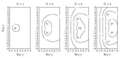
Figure 1. Reflection coefficient computed for the one-dimensional Helmholtz problem with $\gamma\in\{z\in\mathbb{C}|0<\text{Re}(z)<8,-8<\text{Im}(z)<+8\}$ in $(-1,0)$ with the ABC of type $(1,N)$ with $\gamma_{1}=1$ applied in $(0,1)$, where $N\in\{1,2,3,4\}$. A $Q_{N}$ Lagrange finite element with $N$-point reduced integration was used in $(-1,0)$ as well as in $(0,1)$. For each $N\in\{1,2,3,4\}$, the reflection coefficient virtually vanished where $\gamma/\gamma_{1}$ coincided with the zeros of $[N/N]_{\exp{(-z)}}$; those points are shown with the $+$ symbols.

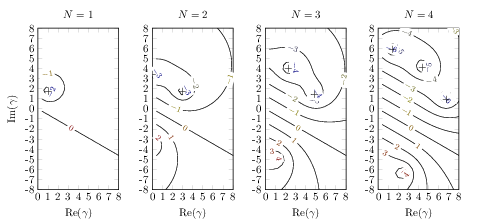
Figure 2. Reflection coefficient computed for the one-dimensional Helmholtz problem with $\gamma\in\{z\in\mathbb{C}|0<\text{Re}(z)<8,-8<\text{Im}(z)<+8\}$ in $(-1,0)$ with the ABC of type $(1,N)$ with $\gamma_{1}=1/2+\sqrt{3}/2\!\cdot\!\mathfrak{i}$ applied in $(0,1)$, where $N\in\{1,2,3,4\}$. A $Q_{N}$ Lagrange finite element with $N$-point reduced integration was used in $(-1,0)$ as well as in $(0,1)$. For each $N\in\{1,2,3,4\}$, the reflection coefficient virtually vanished where $\gamma/\gamma_{1}$ coincided with the zeros of $[N/N]_{\exp{(-z)}}$; those points are shown with the $+$ symbols.

7.1. One-dimensional examples

In this section we numerically verify the formula for the reflection coefficient (81) for ABCs of type $(1,N)$.

We consider a one-dimensional domain, $D^{\textrm{1D}}:=(-1,1)$, in which the physical domain and the artificial domain are defined to be $(-1,0)$ and $(0,1)$, respectively. We consider a mesh $\mathcal{T}^{\textrm{1D}}$ of $D^{\textrm{1D}}$ defined as $\mathcal{T}^{\textrm{1D}}:=\{[-1,0],[0,1]\}$; i.e., we have one absorbing layer, $[0,1]$. We then define function spaces on $\mathcal{T}^{\textrm{1D}}$, $V^{\textrm{1D}}$ and $V^{\textrm{1D}}_{0}$, as:

$$V^{\textrm{1D}}: =\{w\in H^{1}(D^{\textrm{1D}})|w_{|K}\in\mathbb{P}_{N},\forall K\in\mathcal{T}^{\textrm{1D}}\},$$ (93a)

$$V^{\textrm{1D}}_{0}: =\{w\in V^{\textrm{1D}}|w(\pm 1)=0\},$$ (93b)

where $\mathbb{P}_{N}$ is the space of univariate polynomials of degree $N$. We use the $Q_{N}$, or $P_{N}$, Lagrange finite element with the Gauss-Lobatto nodes. We then consider the following problem:

Find $$u^{\textrm{1D}}\in V^{\textrm{1D}}$$ such that

$$\fint_{D^{\textrm{1D}}}\frac{\gamma^{2}}{g^{\textrm{1D}}}u^{\textrm{1D}}\overline{w^{\textrm{1D}}}+g^{\textrm{1D}}u_{,x}^{\textrm{1D}}\overline{w_{,x}^{\textrm{1D}}}\thinspace\mathrm{d}x =0\quad\forall w^{\textrm{1D}}\in V^{\textrm{1D}}_{0},$$ (94b)

$$u^{\textrm{1D}}(+1) =0,$$ (94c)

$$u^{\textrm{1D}}(-1) =1,$$ (94d)

where:

$$g^{\textrm{1D}}(x):=\left\{\begin{array}[]{cl}\gamma_{0},&x\leq 0,\\ \gamma_{1},&\textrm{otherwise},\end{array}\right.$$ (97)

where $\gamma_{0}=1$ and $\gamma_{1}\in\mathbb{C}$. Note that we use $N$-point reduced integration in the physical domain $(-1,0)$ as well as in the artificial domain $(0,1)$. (94c) is the termination condition for the proposed ABC and (94d) is the standard Dirichlet boundary condition.

We solved (94) for $\gamma_{1}\in\{1,1/2+\sqrt{3}/2\!\cdot\!\mathfrak{i}\}$ for $N\in\{1,2,3,4\}$ for $\gamma\in\{z\in\mathbb{C}|0<\text{Re}(z)<8,-8<\text{Im}(z)<+8\}$ using Firedrake. We used MUMPS parallel sparse direct solver [5, 6] via PETSc. For each case, to compute the the reflection coefficient for the discrete wave solution (81) numerically, we decomposed the computed solution into the incoming/growing discrete wave component and the outgoing/decaying discrete wave component directly inspecting the finite element local matrix associated with $K=[-1,0]\in\mathcal{T}^{\textrm{1D}}$ required to assemble (94b); see [30, 34] for details. Fig. 1 and Fig. 2 show the contour plots of the computed reflection coefficients for $N\in\{1,2,3,4\}$, for $\gamma_{1}=1$ and $\gamma_{1}=1/2+\sqrt{3}/2\!\cdot\!\mathfrak{i}$, respectively. One can observe that these contour plots agree with the formula (81). Specifically, for each $\gamma_{1}$, for each $N$, we verified that the reflection coefficient vanished at which $\gamma/\gamma_{1}$ coincided with the zeros of $[N/N]_{\exp{(-z)}}$; Table 1 lists the zeros of $[N/N]_{\exp{(-z)}}$ for $N\in\{1,2,3,4\}$.

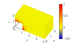
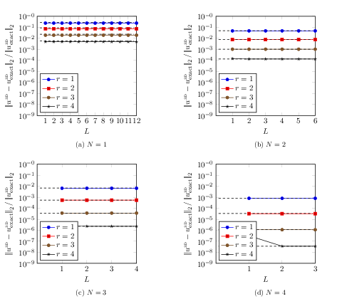
Figure 3. Exact solution to the example Helmholtz problem with $s=+4.00+0.25\mathfrak{i}$.

Figure 4. Relative $L^{2}$-norm errors from ABCs of type $(L,N)$ for $s=+4.00+0.25\mathfrak{i}$: (a) $N=1$, (b) $N=2$, (c) $N=3$, and (d) $N=4$. $r\in\{1,2,3,4\}$ represents the refinement level. $L$ was chosen for each $N$ so that $(LN)_{\textrm{max}}\leq 12$. Estimated discretisation errors are also shown with black dashed lines.

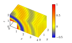
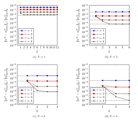
Figure 5. Exact solution to the example Helmholtz problem with $s=+0.25+4.00\mathfrak{i}$.

Figure 6. Relative $L^{2}$-norm errors from ABCs of type $(L,N)$ for $s=+0.25+4.00\mathfrak{i}$: (a) $N=1$, (b) $N=2$, (c) $N=3$, and (d) $N=4$. $r\in\{1,2,3,4\}$ represents the refinement level. $L$ was chosen for each $N$ so that $(LN)_{\textrm{max}}\leq 12$. Estimated discretisation errors are also shown with black dashed lines.

Figure 7. Exact solution to the example Helmholtz problem with $s=+4.00\mathfrak{i}$.

Figure 8. Relative $L^{2}$-norm errors from ABCs of type $(L,N)$ for $s=+4.00\mathfrak{i}$: (a) $N=1$, (b) $N=2$, (c) $N=3$, and (d) $N=4$. $r\in\{1,2,3,4\}$ represents the refinement level. $L$ was chosen for each $N$ so that $(LN)_{\textrm{max}}\leq 12$. Estimated discretisation errors are also shown with black dashed lines.

7.2. Three-dimensional examples

In this section we follow the standard approach [13, 23] to extend the one-dimensional formulation of the proposed ABC introduce in Sec. 6 to three dimensions.

We consider a three-dimensional ($d=3$) domain $D^{\textrm{3D}}$ defined as $D^{\textrm{3D}}:=\{\boldsymbol{x}\in^{3}|\boldsymbol{x}\in\prod_{i\in\{1,2,3\}}(0,B_{i}+Lh)\textrm{ and }\boldsymbol{x}\not\in[0,1]^{3}\}$, representing a box with a cubic hole, where $(B_{1},B_{2},B_{3})=(4,2,2)$ and $h=2^{-\textrm{ref}}$ with $\textrm{ref}\in\mathbb{N}$ being the refinement level. The physical domain is given as $\{\boldsymbol{x}\in^{3}|\boldsymbol{x}\in\prod_{i\in\{1,2,3\}}(0,B_{i})\textrm{ and }\boldsymbol{x}\not\in[0,1]^{3}\}$, and we are to use an ABC of type $(L,N)$ in the artificial domain in each direction. We let $\partial D^{\textrm{3D}}_{0}:=\{\boldsymbol{x}\in\partial D^{\textrm{3D}}|x_{i}=B_{i}+Lh\textrm{ for some }i\in\{0,1,2\}\}$, $\partial D^{\textrm{3D}}_{1}:=\{\boldsymbol{x}\in\partial D^{\textrm{3D}}|\boldsymbol{x}\in[0,1]^{3}\}$, and $\partial D^{\textrm{3D}}_{2}:=\{\boldsymbol{x}\in\partial D^{\textrm{3D}}|x_{i}=0\textrm{ for some }i\in\{0,1,2\}\}$. We consider a mesh $\mathcal{T}^{\textrm{3D}}$ of $D^{\textrm{3D}}$ composed of cuboids of edge lengths $h$. We then define function spaces on $\mathcal{T}^{\textrm{3D}}$, $V^{\textrm{3D}}$ and $V^{\textrm{3D}}_{0}$, as:

$$V^{\textrm{3D}}: =\{w\in H^{1}(D^{\textrm{3D}})|w_{|K}\in\mathbb{Q}_{N,d},\forall K\in\mathcal{T}^{\textrm{3D}}\},$$ (98a)

$$V^{\textrm{3D}}_{0}: =\{w\in V^{\textrm{3D}}|w_{|\partial D^{\textrm{3D}}_{0}\cup\partial D^{\textrm{3D}}_{1}}=0\},$$ (98b)

where $\mathbb{Q}_{N,d}$ is the space of $d$-variate polynomials of degree with respect to each variable at most $N$. We use the $Q_{N}$ tensor-product Lagrange finite element with the Gauss-Lobatto nodes in each direction. We then consider the following problem whose solution is to converge to the exact solution in the physical domain given as:

$$u^{\textrm{3D}}_{\textrm{exact}}=\frac{e^{-s\left|\!\left|x\right|\!\right|}}{\left|\!\left|x\right|\!\right|}:$$ (99)

Find $$u^{\textrm{3D}}\in V^{\textrm{3D}}$$ such that

$$\int_{D^{\textrm{3D}}}\frac{1}{\prod\limits_{i\in\{0,1,2\}}g^{\textrm{3D}}_{i}}\left(s^{2}u^{\textrm{3D}}\overline{w^{\textrm{3D}}}+\sum_{i\in\{0,1,2\}}(g^{\textrm{3D}}_{i})^{2}u_{,i}^{\textrm{3D}}\overline{w_{,i}^{\textrm{3D}}}\right)\thinspace\mathrm{d}\boldsymbol{x} =0,\quad\forall w^{\textrm{3D}}\in V^{\textrm{3D}}_{0},$$ (100b)

$${u^{\textrm{3D}}}_{|\partial D^{\textrm{3D}}_{0}} =0,$$ (100c)

$${u^{\textrm{3D}}}_{|\partial D^{\textrm{3D}}_{1}} =\mathcal{I}(u^{\textrm{3D}}_{\textrm{exact}}),$$ (100d)

where, for $i\in\{1,2,3\}$:

$$g^{\textrm{3D}}_{i}(x_{i}):=\left\{\begin{array}[]{cl}\gamma_{0},&x_{i}\leq B_{i},\\ \gamma_{l},&B_{i}+(l-1)h<x_{i}\leq B_{i}+lh,\quad l\in\{1,\cdots,L\},\end{array}\right.$$ (103)

where $\gamma_{0}=1$ and:

$$\gamma_{l}=\left(\cos\phi_{l}\!\cdot\!s+\frac{\sin^{2}\phi_{l}}{\cos\phi_{l}}\right)\!\cdot\!\frac{1}{N+1}\!\cdot\!h,\quad\phi_{l}\in\left[0,\frac{\pi}{2}\right),\quad l\in\{1,\cdots,L\}.$$ (104)

In (104) the term in the parentheses was proposed in [25] for the CRBCs for the case corresponding to $N=1$; as optimisation of the ABC parameters is outside the scope of this paper, we use this formula for all $N$, simply choosing $\phi_{l}$ in $[0,\pi/2)$ according to the $L$-point Gauss-Legendre quadrature. The factors $1/(N+1)$ and $h$ were introduced specifically for the proposed ABC to normalise $\gamma_{l}$ across different values of $N$ and across different refinement levels, respectively. Although the standard symbol was used for the integral in (100b) for simplicity, we only use the full integration rule in the physical domain, and use the $N$-point reduced integration rule in $x_{i}>B_{i}$ in the $x_{i}$-direction for each $i\in\{1,2,3\}$. (100c) is the termination condition for the ABC and (100d) is the standard Dirichlet boundary condition, where $\mathcal{I}:C^{0}(D^{\textrm{3D}})\rightarrow V^{\textrm{3D}}$ is the interpolation operator from $C^{0}(D^{\textrm{3D}})$ to $V^{\textrm{3D}}$. The homogeneous Neumann boundary condition was weakly applied on $\partial D^{\textrm{3D}}_{2}$ in (100b).

We solved the above problem for $s\in\{+4.00+0.25\mathfrak{i},+0.25+4.00\mathfrak{i},+4.00\mathfrak{i}\}$. For each $s$, we used four different finite element degrees, $N\in\{1,2,3,4\}$, and for each $N$, we considered four different refinement levels, $\textrm{ref}\in{1,2,3,4}$. For each case, we varied the number of absorbing layers, $L$, so that $LN\leq 12$. We used MUMPS parallel sparse direct solver [5, 6] via PETSc unless $(N,\textrm{ref})=(4,4)$. For $(N,\textrm{ref})=(4,4)$, via PETSc, we used the Generalized Minimal Residual method (KSPGMRES) with the block Jacobi preconditioning (PCBJACOBI) with the sub KSP type KSPPREONLY and with the sub PC type the incomplete factorization preconditioners (PCILU) or the successive over relaxation (PCSOR). The use of more elaborated preconditioners will be explored elsewhere. For each case, we computed the relative $L^{2}$-norm error, $\left|\!\left|u^{\textrm{3D}}-u^{\textrm{3D}}_{\textrm{exact}}\right|\!\right|_{2}/\left|\!\left|u^{\textrm{3D}}_{\textrm{exact}}\right|\!\right|_{2}$, in the physical domain. Fig. 4, Fig. 6, and Fig. 8 show the exact solutions for $s=+4.00+0.25\mathfrak{i}$, $s=+0.25+4.00\mathfrak{i}$, and $s=+4.00\mathfrak{i}$. Fig. 4, Fig. 6, and Fig. 8, show the plots of the computed relative $L^{2}$-norm errors for $s=+4.00+0.25\mathfrak{i}$, $s=+0.25+4.00\mathfrak{i}$, and $s=+4.00\mathfrak{i}$, respectively, for each $N$, for each ref. For each $s$, for each pair of $N$ and ref, we computed the interpolation error $\left|\!\left|\mathcal{I}(u^{\textrm{3D}}_{\textrm{exact}})-u^{\textrm{3D}}_{\textrm{exact}}\right|\!\right|_{2}/\left|\!\left|u^{\textrm{3D}}_{\textrm{exact}}\right|\!\right|_{2}$ as an indicator of the discretisation error. The interpolation error is shown with the black dotted line for each case. The figures indicate that, for each $s$, with $N$ and ref fixed, the relative $L^{2}$-norm error decreases sharply to the discretisation error as $L$ increases. Such sharp convergence of the error is typically observed with PMDLs and CRBCs.

8. Conclusion and future works

We proposed a new class of ABCs for the Helmholtz equation, which is parametrised by a tuple $(L,N)$; The ABCs of type $(L,N)$ are derived from the layerwise constant PMLs with $L$ absorbing layers using the $Q_{N}$ finite element in conjunction with the $N$-point Gauss-Legendre quadrature reduced integration. The proposed ABCs generalise the PMDLs [23], including them as type $(L,1)$, which is known to outperform the standard PMLs and to show equivalent performances to the CRBCs [25], in terms of the accuracy and also in terms of the insensitivity to the choice of the parameters. The proposed ABCs of type $(L,N)$ inherit these favourable properties. Like the PMDLs, the proposed ABCs only involve a single Helmholtz-like equation over the entire computational domain, even in existence of edges and corners. As a generalisation of the PMDLs, for any $N\in\mathbb{N}$, the proposed ABCs allow for a monolithic discretisation of the physical and the artificial domains as long as a $Q_{N}$ finite element is used in the physical domain. These features were validated in the one- and three-dimensional numerical examples. Moreover, having given more insight, the analysis that we performed in this work using the Jacobi polynomials strongly motivated by [2] potentially advance the fields of ABCs in related areas.

The ABCs of type $(L,N)$ and those of type $(LN,1)$ introduce the same number of auxiliary degrees of freedom in the artificial domain and achieve the same order of accuracy. However, as the latter involve $LN$ complex parameters while the former only involve $L$, one will have a finer control of the absorption profile when using the latter, which might be advantageous if, e.g., one had a good a priori knowledge of the target solution; see also [22]. Note also that the matrix structure of the former is denser than that of the latter in the artificial domain as the former use the $Q_{N}$ finite elements and the latter use the $Q_{1}$ finite elements; this could potentially be a drawback of using the former if the size of the artificial domain was comparable with that of the physical domain.

With regard to the proposed ABCs, we have yet to investigate various aspects that have been studied for the PMDLs, the CRBCs, and the other related ABCs, including applications to the wave equation [19, 24, 25], to the elastodynamics [8], to the other elasticity problems [35, 36], and to the problems with polygonal domains [23]. For the Helmholtz and the other equations, we are also interested in using different families of finite elements in conjunction with some reduced integration rules in the artificial domain, so that the ABCs can be applied with no added cost of implementation when those families of elements are used for discretisation in the physical domain. These ideas will be explored in the future works.

Code availability

The exact version of Firedrake used, along with all of the scripts employed in the experiments presented in this paper has been archived on Zenodo [37].

References

- [1] Mark Ainsworth, Discrete Dispersion Relation for hp -Version Finite Element Approximation at High Wave Number, SIAM J. Numer. Anal. 42 (2004), no. 2, 553–575.
- [2] by same author, Dispersive and dissipative behaviour of high order discontinuous Galerkin finite element methods, Journal of Computational Physics 198 (2004), no. 1, 106–130.
- [3] by same author, Dispersive behaviour of high order finite element schemes for the one-way wave equation, Journal of Computational Physics 259 (2014), 1–10.
- [4] Mark Ainsworth and Hafiz Abdul Wajid, Optimally Blended Spectral-Finite Element Scheme for Wave Propagation and NonStandard Reduced Integration, SIAM J. Numer. Anal. 48 (2010), no. 1, 346–371.
- [5] Patrick R. Amestoy, Iain S. Duff, Jean-Yves L’Excellent, and Jacko Koster, A fully asynchronous multifrontal solver using distributed dynamic scheduling, SIAM Journal on Matrix Analysis and Applications 23 (2001), no. 1, 15–41.
- [6] Patrick R. Amestoy, Abdou Guermouche, Jean-Yves L’Excellent, and Stéphane Pralet, Hybrid scheduling for the parallel solution of linear systems, Parallel Computing 32 (2006), no. 2, 136–156, Parallel Matrix Algorithms and Applications (PMAA’04).
- [7] Sergey Asvadurov, Vladimir Druskin, Murthy N. Guddati, and Leonid Knizhnerman, On Optimal Finite-Difference Approximation of PML, SIAM Journal on Numerical Analysis 41 (2003), no. 1, 287–305.
- [8] Daniel Baffet, Jacobo Bielak, Dan Givoli, Thomas Hagstrom, and Daniel Rabinovich, Long-time stable high-order absorbing boundary conditions for elastodynamics, Computer Methods in Applied Mechanics and Engineering 241-244 (2012), 20–37.
- [9] Satish Balay, Shrirang Abhyankar, Mark F. Adams, Steven Benson, Jed Brown, Peter Brune, Kris Buschelman, Emil Constantinescu, Lisandro Dalcin, Alp Dener, Victor Eijkhout, William D. Gropp, Václav Hapla, Tobin Isaac, Pierre Jolivet, Dmitry Karpeev, Dinesh Kaushik, Matthew G. Knepley, Fande Kong, Scott Kruger, Dave A. May, Lois Curfman McInnes, Richard Tran Mills, Lawrence Mitchell, Todd Munson, Jose E. Roman, Karl Rupp, Patrick Sanan, Jason Sarich, Barry F. Smith, Stefano Zampini, Hong Zhang, Hong Zhang, and Junchao Zhang, PETSc/TAO users manual, Tech. Report ANL-21/39 - Revision 3.16, Argonne National Laboratory, 2021.
- [10] Satish Balay, Shrirang Abhyankar, Mark F. Adams, Steven Benson, Jed Brown, Peter Brune, Kris Buschelman, Emil M. Constantinescu, Lisandro Dalcin, Alp Dener, Victor Eijkhout, William D. Gropp, Václav Hapla, Tobin Isaac, Pierre Jolivet, Dmitry Karpeev, Dinesh Kaushik, Matthew G. Knepley, Fande Kong, Scott Kruger, Dave A. May, Lois Curfman McInnes, Richard Tran Mills, Lawrence Mitchell, Todd Munson, Jose E. Roman, Karl Rupp, Patrick Sanan, Jason Sarich, Barry F. Smith, Stefano Zampini, Hong Zhang, Hong Zhang, and Junchao Zhang, PETSc Web page, 2021.
- [11] Satish Balay, William D. Gropp, Lois Curfman McInnes, and Barry F. Smith, Efficient management of parallelism in object oriented numerical software libraries, Modern Software Tools in Scientific Computing (E. Arge, A. M. Bruaset, and H. P. Langtangen, eds.), Birkhäuser Press, 1997, pp. 163–202.
- [12] Alvin Bayliss and Eli Turkel, Radiation boundary conditions for wave-like equations, Comm. Pure Appl. Math. 33 (1980), no. 6, 707–725.
- [13] Jean-Pierre Berenger, A perfectly matched layer for the absorption of electromagnetic waves, Journal of Computational Physics 114 (1994), no. 2, 185–200.
- [14] David S. Bindel and Sanjay Govindjee, Elastic PMLs for resonator anchor loss simulation, Int. J. Numer. Meth. Engng 64 (2005), no. 6, 789–818 (en).
- [15] Garrett. Birkhoff and Richard S. Varga, Discretization errors for well-set Cauchy problems, Journal of Mathematics and Physics 44 (1965), 1–23.
- [16] Weng Cho Chew and William H. Weedon, A 3d perfectly matched medium from modified maxwell’s equations with stretched coordinates, Microwave and Optical Technology Letters 7 (1994), no. 13, 599–604.
- [17] Björn Engquist and Andrew Majda, Absorbing boundary conditions for numerical simulation of waves, Proc. Natl. Acad. Sci. U.S.A. 74 (1977), no. 5, 1765–1766.
- [18] Bjorn Engquist and Andrew Majda, Radiation boundary conditions for acoustic and elastic wave calculations, Comm. Pure Appl. Math. 32 (1979), no. 3, 313–357.
- [19] Dan Givoli and Beny Neta, High-order non-reflecting boundary scheme for time-dependent waves, Journal of Computational Physics 186 (2003), no. 1, 24–46.
- [20] I. S Gradshtein, Table of integrals, series, and products, 8 ed., Academic Press, 2014.
- [21] Murthy N. Guddati, Arbitrarily wide-angle wave equations for complex media, Computer Methods in Applied Mechanics and Engineering 195 (2006), no. 1-3, 65–93.
- [22] Murthy N. Guddati, Vladimir Druskin, and Ali Vaziri Astaneh, Exponential convergence through linear finite element discretization of stratified subdomains, Journal of Computational Physics 322 (2016), 429–447 (en).
- [23] Murthy N. Guddati and Keng-Wit Lim, Continued fraction absorbing boundary conditions for convex polygonal domains, Int. J. Numer. Meth. Engng 66 (2006), no. 6, 949–977.
- [24] Thomas Hagstrom and Timothy Warburton, A new auxiliary variable formulation of high-order local radiation boundary conditions: corner compatibility conditions and extensions to first-order systems, Wave Motion 39 (2004), no. 4, 327–338.
- [25] by same author, Complete Radiation Boundary Conditions: Minimizing the Long Time Error Growth of Local Methods, SIAM J. Numer. Anal. 47 (2009), no. 5, 3678–3704.
- [26] David A. Ham, Paul H. J. Kelly, Lawrence Mitchell, Colin J. Cotter, Robert C. Kirby, Koki Sagiyama, Nacime Bouziani, Sophia Vorderwuelbecke, Thomas J. Gregory, Jack Betteridge, Daniel R. Shapero, Reuben W. Nixon-Hill, Connor J. Ward, Patrick E. Farrell, Pablo D. Brubeck, India Marsden, Thomas H. Gibson, Miklós Homolya, Tianjiao Sun, Andrew T. T. McRae, Fabio Luporini, Alastair Gregory, Michael Lange, Simon W. Funke, Florian Rathgeber, Gheorghe-Teodor Bercea, and Graham R. Markall, Firedrake user manual, Imperial College London and University of Oxford and Baylor University and University of Washington, first edition ed., 5 2023.
- [27] Robert L Higdon, Absorbing Boundary Conditions for Difference Approximations to the Multi-Dimensional Wave Equation, Math. Comp. 47 (1986), 437–459.
- [28] by same author, Numerical Absorbing Boundary Conditions for the Wave Equation, Math. Comp. 49 (1987), 65–90.
- [29] Robert C. Kirby, Andreas Klöckner, and Ben Sepanski, Finite Elements for Helmholtz Equations with a Nonlocal Boundary Condition, SIAM J. Sci. Comput. 43 (2021), no. 3, A1671–A1691.
- [30] Tsuyoshi Koyama, Efficient Evaluation of Damping in Resonant MEMS, Ph.D. thesis, University of California, Berkeley (2008).
- [31] Axel Modave, Andreas Atle, Jesse Chan, and Timothy Warburton, A GPU-accelerated nodal discontinuous Galerkin method with high-order absorbing boundary conditions and corner/edge compatibility: A GPU-accelerated DG method with HABCs and corner/edge compatibility, Int J Numer Methods Eng 112 (2017), no. 11, 1659–1686.
- [32] Florian Rathgeber, David A. Ham, Lawrence Mitchell, Michael Lange, Fabio Luporini, Andrew T. T. McRae, Gheorghe-Teodor Bercea, Graham R. Markall, and Paul H. J. Kelly, Firedrake: automating the finite element method by composing abstractions, ACM Trans. Math. Softw. 43 (2016), no. 3, 24:1–24:27.
- [33] Edward B. Saff and Richard S. Varga, On the zeros and poles of padé approximants to , Numerische Mathematik 25 (1975), 1–14.
- [34] Koki Sagiyama, Sanjay Govindjee, and Per-Olof Persson, An efficient time-domain perfectly matched layers formulation for elastodynamics on spherical domains, International Journal for Numerical Methods in Engineering 100 (2014), no. 6, 419–441.
- [35] Siddharth Savadatti and Murthy N. Guddati, Accurate absorbing boundary conditions for anisotropic elastic media. Part 1: Elliptic anisotropy, Journal of Computational Physics 231 (2012), no. 22, 7584–7607.
- [36] by same author, Accurate absorbing boundary conditions for anisotropic elastic media. Part 2: Untilted non-elliptic anisotropy, Journal of Computational Physics 231 (2012), no. 22, 7608–7625.
- [37] Software used in ‘Absorbing boundary conditions for the Helmholtz equation using Gauss-Legendre quadrature reduced integrations’, aug 2023.