How Safe Am I Given What I See?
Calibrated Prediction of Safety Chances for Image-Controlled Autonomy

Abstract

End-to-end learning has emerged as a major paradigm for developing autonomous controllers. Unfortunately, with its performance and convenience comes an even greater challenge of safety assurance. A key factor in this challenge is the absence of low-dimensional and interpretable dynamical states, around which traditional assurance methods revolve. Focusing on the online safety prediction problem, this paper systematically investigates a flexible family of learning pipelines based on generative world models, which do not require low-dimensional states. To implement these pipelines, we overcome the challenges of missing safety labels under prediction-induced distribution shift and learning safety-informed latent representations. Moreover, we provide statistical calibration guarantees for our safety chance predictions based on conformal inference. An extensive evaluation of our predictor family on two image-controlled case studies, a racing car and a cartpole, delivers counterintuitive results and highlights open problems in deep safety prediction.

1 Introduction

To handle the complexity of the real world, autonomous systems increasingly rely on high-resolution sensors such as cameras and lidars, as well as large learning architectures to process the sensing data. It has become increasingly commonplace to use end-to-end reinforcement and imitation learning (Codevilla et al. 2018; Tomar et al. 2022; Betz et al. 2022), conveniently bypassing conventional intermediate components such as state estimation and planning. While end-to-end learning can produce sophisticated behaviors from large raw datasets, it complicates safety assurance of such autonomous systems (Fulton et al. 2019).

Traditional approaches to ensure safety (e.g., that a car does not hit an obstacle) predominantly rely on the notion of a low-dimensional state with a physical meaning (e.g., the car’s position and velocity). For example, reachability analysis propagates the system’s state forward (Bansal et al. 2017; Chen and Sankaranarayanan 2022), barrier functions synthesize safe low-dimensional controllers (Ames et al. 2019; Xiao, Cassandras, and Belta 2023), and trajectory predictors output future states of agents (Salzmann et al. 2020; Teeti et al. 2022). These methods do not straightforwardly scale to image-based controllers with thousands of inputs without an exact physical interpretation. Instead, model-based approaches require abstractions of sensing and perception to take images into account. These abstractions are either system-specific and effortful to build (e.g., modeling the ray geometry behind pixel values (Santa Cruz and Shoukry 2022)) or simplified and potentially inaccurate (e.g., a linear overapproximation of visual perception (Hsieh et al. 2022)).

The problem raised in this paper is the reliable online prediction of safety for an autonomous system with an image-based controller without access to a physically meaningful low-dimensional dynamical state or model. For instance, given an image, what is the probability that a racing car stays within the track’s bounds within 5 seconds after the image was taken? In this context, the reliability requirement, also known as calibration (Guo et al. 2017), would be to provide an upper bound on the difference between the estimated and true probability. Devoid of typical dynamical models, this setting calls for a careful combination of image-based prediction and statistical guarantees. Existing works focus on learning to control rather than assuring image-based systems (Hafner et al. 2019), assume access to a true low-dimensional initial state (Lindemann et al. 2023), or do not provide any reliability guarantees (Acharya, Russell, and Ahmed 2022). Nonetheless, reliably solving the prediction problem would enable downstream safety interventions like handing the control off to a human or switching to a fallback controller, which are outside of this paper’s scope.

This paper proposes a family of learning pipelines for the formalized safety prediction problem, shown in Fig. 1. The proposed family offers flexible modularity (e.g., whether it uses intermediate representations) and tunable specificity to a particular controller. Some of these pipelines repurpose the latest generative architectures for reinforcement learning, known as world models (Ha and Schmidhuber 2018), for online prediction of future images from the recent ones. World models tend to produce distribution-shifted image forecasts, which poses a challenge to evaluating the safety of these forecasts. We address this challenge by using robust vision features and data augmentation — and also investigate using safety labels to regularize latent representations learned by the world models.

To provide calibration guarantees, we combine post-hoc calibration (Zhang, Kailkhura, and Han 2020) with the recently popularized distribution-free technique of conformal prediction (Vovk, Gammerman, and Shafer 2005; Lei et al. 2018). This enables us to tune the predictive safety probabilities orthogonally to the design choices within the prediction pipeline and provide statistical bounds for them from validation data.

We perform extensive experiments on two popular benchmarks in the OpenAI Gym (Brockman et al. 2016): racing car and cart pole. We particularly focus on long-horizon predictions, which leads us to counterintuitive results on the impact of modularity and controller-specificity in our family of learning-based prediction pipelines. Our experiments also show that predicting well-calibrated safety chances is easier than safety labels over longer horizons.

In summary, this paper makes three contributions:

1. A flexible family of learning pipelines for online safety prediction in image-controlled autonomous systems.

2. A conformal post-hoc calibration technique with statistical guarantees on safety chance predictions.

3. An extensive experimental evaluation of our predictor family on two case studies.

After describing the problem and notation in Sec. 2, we introduce our family of prediction approaches in Sec. 3. The case studies and their results are presented in Sec. 4, after which we review the related work in Sec. 5 and conclude.

2 Preliminaries

This section introduces the necessary notation and describes the problem addressed in this paper.

Problem Setting

Definition 1 (Dynamical system).

A discrete-time dynamical system $s=(\mathbf{X},\mathbf{Z},\mathbf{U},\emph{h},f,o,x_{0},\varphi)$ consists of:

• State space $\mathbf{X}$, containing continuous states $x$

• Observation space $\mathbf{Z}$, containing images $y$

• Action space $\mathbf{U}$, with discrete/continuous commands $u$

• Image-based controller $\emph{h}:\mathbf{\mathbf{Z}}\rightarrow\mathbf{\mathbf{U}}$, typically implemented by a neural network

• Dynamical model $f:\mathbf{X}\times\mathbf{U}\rightarrow\mathbf{X}$ , which sets the next state from a past state and an action (unknown to us)

• Observation model $o:\mathbf{X}\rightarrow\mathbf{Z}$, which generates an observation based on the state (unknown to us)

• Initial state $x_{0}$, from which the system starts executing

• State-based safety property $\varphi:\mathbf{X}\rightarrow\{0,1\}$, which determines whether a given state $x$ is safe

We focus on systems with observation spaces with thousands of pixels and unknown non-linear dynamical and observation models. In such systems, while the state space $\mathbf{X}$ is conceptually known (if only to define $\varphi$), it is not necessary (and often difficult) to construct $f$ and $o$ because the controller acts directly on the observation space $\mathbf{Z}$. Without relying on $f$ and $o$, end-to-end methods like deep reinforcement learning (Mnih et al. 2015) and imitation learning (Hussein et al. 2017) are used to train a controller h by using data from the observation space. Once the controller is deployed in state $x_{0}$, the system executes a trajectory, which is a sequence $\{x_{i},y_{i},u_{i}\}^{t}_{i=0}$ up to time $t$, where:

$$x_{i+1}=f(x_{i},u_{i}),\quad y_{i}=o(x_{i}),\quad u_{i}=\emph{h}(y_{i})$$ (1)

Instead of using this model, we extract predictive information from three sources of data. First, we will use the current observation, $y_{i}$, at some time $i$. For example, when a car is at the edge of the track, it has a higher probability of being unsafe in the next few steps. Second, past observations $y_{i-m+1},\dots,y_{i}$ provide dynamically useful features that can only be extracted from time series, such as the speed and direction of motion. For example, just before a car enters a turn, the sequence of past observations implicitly informs how hard it will be to remain safe. Third, not only do observations inform safety, but so do the controller’s past/present outputs $\emph{h}(y_{i-m+1},\dots,y_{i})$. For instance, if by mid-turn the controller has not changed the steering angle, it may be less likely to navigate this turn safely.

Our goal is to predict the system’s safety $\varphi(x_{i+k})$ at time $i+k$ given a series of $m$ observations $\mathbf{y}_{i}=(y_{i-m+1},...,y_{i})$. This sequence of observations does not, generally, determine the true state $x_{i}$ (e.g., when $m=1$, function $o$ may not be invertible). This leads to partial state observability, which we model stochastically. Specifically, we say that from the predictor’s perspective, $x_{i}$ is drawn from some belief distribution $\mathcal{D}_{\mathbf{y}_{i}}$. This induces a distribution of subsequent trajectories and transforms future safety $\varphi(x_{i+k})$ into a Bernoulli random variable. Therefore, we will estimate the conditional probability $P(\varphi(x_{i+k})\mid\mathbf{y}_{i})$ and provide an error bound on our estimates. Note that process noise in $f_{d}$ and measurement noise in $f_{o}$ are orthogonal to the issue of partial observability; nonetheless, both of these noises are supported by our approach and would be treated as part of the stochastic uncertainty in the future $\varphi$. To sum up the above, we arrive at the following problem description.

Problem (Calibrated safety prediction).

Given horizon $k>0$, confidence $\alpha\in(0,0.5)$, and observations $\mathbf{y}_{i}$ from some system $s$ with unknown $f$ and $o$, estimate future safety chance $P(\varphi(x_{i+k})\mid\mathbf{y}_{i})$ and provide an upper bound for the estimation error that holds in at least $1-\alpha$ cases.

Figure 1: Dynamical system with predictors. Arrows show data flow, and dashes show optional controller dependence.

Predictors and Datasets

To address the above problem we will build two types of predictors: for safety labels and for safety chances.

Definition 2 (Safety label predictor).

For horizon $k>0$, a safety label predictor $\rho:\mathbf{Z}^{m}\rightarrow\{0,1\}$ predicts the safety $\varphi(x_{i+k})$ at time $i+k$.

Definition 3 (Safety chance predictor).

For horizon $k>0$, a safety chance predictor $g:\mathbf{Z}^{m}\rightarrow[0,1]$ predicts the safety chance $P(\varphi(x_{i+k})\mid\mathbf{y}_{i})$ at time $i+k$.

Controller-specific (controller-independent) predictors are trained on observation-controller (observation-action) datasets respectively. Using controller-independent predictors trades off some prediction power for generalizability — and it is the first flexibility dimension (i.e., controller-specificity) in our family of learning pipelines. We compare these two types of predictors in Sec. 4.

To train these predictors, we collect two types of datasets, with a conveniently unified notation $\mathbf{Z}$ and $\mathbf{z}$ to mean either dataset and its elements. The first type in Def. 4 only contains data from a specific controller, while the second in Def. 5 can mix controllers because due to explicit actions.

Definition 4 (Observation-controller dataset).

An observation-controller dataset $\mathbf{Z}=\{(\mathbf{z}_{j},\varphi_{j})~{}|~{}j=1,\dots,N\}$ consists of pairs of $m$-long sequences $\mathbf{z}_{j}:=(y_{i-m},...,y_{i})$ for some time $i$ and safety labels $\varphi_{j}:=\varphi(x_{i+k})$ at $k$ steps later, collected by executing a fixed controller h.

Definition 5 (Observation-action dataset).

An observation-action dataset $\mathbf{Z}=\{(\mathbf{z}_{j},\varphi_{j})~{}|~{}j=1,\dots,N\}$ consists of pairs of $m$-long sequences of paired observations and corresponding actions $\mathbf{z}_{j}=((y_{i-m+1},u_{i-m+1}),...,(y_{i},u_{i}))$, and safety labels $\varphi_{j}:=\varphi(x_{i+k})$ obtained $k$ steps later.

3 Safety Predictor Family

First, we describe how we develop safety label predictors. Then we transform them into safety chance predictors.

Monolithic and Composite Label Predictors

The second dimension of our family of learning pipelines is modularity. In this dimension, we distinguish three types of safety label predictors: monolithic predictors, composite image predictors, and composite latent predictors. The high-level distinction between the monolithic and composite predictors is that the latter end with an evaluator, a separate component that determines the safety of the prediction — as shown in Fig. 1. The predictor structures are summarized in Fig. 2 and explained below.

Monolithic predictors directly determine the future safety property based on the observations, as described in Def. 2. These predictors are essentially binary classifiers that leverage deep vision models (with convolutional layers) and time-series models (with recurrent layers). These models are trained in a supervised way on any training dataset $\mathbf{Z}_{t}$ with a given horizon $k$ with a typical binary classification loss, such as cross-entropy. The key drawback of monolithic predictors is their need to be completely re-trained to change the prediction horizon or tune the hyperparameters.

Typically, a Convolutional Neural Network (CNN) serves as an effective classifier for safety prediction. However, as the prediction horizon increases, CNNs may prove inadequate for processing sequential data. Recurrent Neural Networks, such as Long Short-Term Memory (LSTM) networks  (Lindemann et al. 2021), are burdened by computational demands in such scenarios. To address this, we have incorporated a Variational Autoencoder (VAE) (Kingma and Welling 2014) into the LSTM. The VAE compresses the image sequence into a latent sequence, and an LSTM is employed as the safety predictor. This hybrid model aims to optimize both the representation learning capabilities of VAE and the sequential processing prowess of LSTM for enhanced predictive performance. This kind of monolithic latent predictor is defined as below:

Definition 6 (Monolithic latent predictor).

A monolithic latent predictor consists of two parts: an autoencoder and an LSTM. The autoencoder provides an encoder $e$ and decoder $d$ components that define a latent space $\Theta$ containing state vectors $\theta$. The LSTM works as the safety label predictor (Def. 2) from the latent space $\Theta$.

Figure 2: Our predictors (from top to bottom): monolithic, monolithic latent, composite image-based, and composite latent-based.

A composite predictor consists of multiple learning models. A forecaster model constructs the likely future observations, essentially approximating the dynamics $f$ and observation model $o$. Another binary classifier — an evaluator — judges whether a forecasted observation is safe.

Definition 7 (Composite image predictor).

A composite image predictor consists of two parts: an image forecaster and an evaluator. The image forecaster $f_{g}:\mathbf{Z}^{m}\rightarrow\mathbf{Y}$ predicts the future observation $\hat{y}_{i+k}$ based on past $\mathbf{z}_{i}$, and the evaluator $e:\mathbf{Y}\rightarrow\{0,1\}$ determines the safety of the predicted images $\varphi(\hat{y}_{i+k})$. The composite prediction is $v(f_{g}(\mathbf{z}_{i}))$.

Our implementation of the composite image predictor will use a convolutional LSTM (conv-LSTM) (Shi et al. 2015) as an image forecaster, and a convolutional neural network (CNN) for the evaluator.

Definition 8 (Composite latent predictor).

A composite latent predictor consists of three parts: an autoencoder, a latent forecaster, and an evaluator. The autoencoder provides an encoder $e$ and decoder $d$ components that define a latent space $\Theta$ containing state vectors $\theta$. The latent forecaster $f_{l}:\Theta^{m}\rightarrow\Theta$ predicts the future latent state $\hat{\theta}_{i+k}$ based on past $m$ latent states.

Same as for the image predictor, the evaluator $v:\mathbf{Y}\rightarrow\{0,1\}$ operates over the images obtained from the predicted latent states by the decoder. The composite prediction is $v(d(f_{l}(e(\mathbf{z}_{i}))))$.

We implement the encoder/decoder using a Variational Autoencoder (VAE) (Kingma and Welling 2014). The latent forecasting is performed using a Long-Short Term Memory (LSTM) network (Lindemann et al. 2021), and the evaluator, as above, is a CNN.

Training Process

Monolithic predictors $\rho$, evaluators $v$, and image forecasters $f_{g}$ are trained in a supervised manner on a training dataset $\mathbf{Z}_{t}$ containing observation sequences with associated safety labels or future images respectively. Latent forecasters $f_{l}$ are trained on future latent vectors, obtained from true future observations with a VAE encoder $e$, which is trained as described below. The mean squared error (MSE) loss is implemented for the LSTM latent forecaster and conv-LSTM image forecaster, while the monolithic predictors and evaluators use cross entropy (CE) as the loss function. We also implement the early stopping strategy to reduce the learning rate as the total loss drop slows — and stop the training when it reaches below a given threshold.

For the VAE, the total loss $\mathcal{L}$ consists of three parts. The first is the reconstruction loss $\mathcal{L}_{recon}$, which quantifies how well an original image $y$ is approximated by $d(e(y))$ using the MSE loss. The second is the latent loss $\mathcal{L}_{latent}$, which uses Kullback-Leibler divergence loss to minimize the difference between two latent-vector probability distributions $e(y\mid\theta)\approx d(\theta\mid y)$, where $\theta$ is a latent vector and $y$ is an input. In order to preserve the information about safety in latent state representations, we add an optional safety loss $\mathcal{L}_{safety}$, which is a cross entropy loss based on the true safety $\varphi_{i}$ truth of the original images $y_{i}$ and the safety evaluation of the reconstructed images:

$$\mathcal{L}_{safety}=\mathcal{L}_{CE}(v(d(e(y_{i}))),\varphi_{i})$$ (2)

So the total loss function for VAE combines the three parts with regularization parameters $\lambda_{1}$, $\lambda_{2}>0$:

$$\mathcal{L}=\mathcal{L}_{recon}+\lambda_{1}\mathcal{L}_{latent}+\lambda_{2}\mathcal{L}_{safety}$$ (3)

One challenge is that the safety label balance changes in $\mathbf{Z}_{t}$ with the prediction horizon $k$, leading to imbalanced data for higher horizons. To ensure a balanced label distribution, we resample with replacement for a 1:1 safe:unsafe class balance both in the training and testing datasets.

Figure 3: Upper: Car observations, L to R: safe car from $\mathbf{Z}$, unsafe car from $\mathbf{Z}$, safe car from $d$ ($f_{l}$ ($e$ ($\mathbf{Z}$))), safe car from $f_{g}$ ($\mathbf{Z}$). Lower: Cart pole observations. In both rows, the two rightmost images are distribution-shifted.

Another challenge is the distribution shift between the original and forecasted images produced by label predictor $\rho$. The issue is that the forecasted images are distorted (e.g., see the two rightmost images in Fig. 3) and they do not automatically come with safety labels because they are sampled from the forecasted space without a physical ground truth. However, we need to train high-performance evaluators on the forecasted images, as per Fig. 2.

To overcome the distribution shift, we implement two specialized evaluators. One uses a vision approach based on robust domain-specific features of the image. For example, for the racing car case study, we take advantage of the fixed location of the car in the image and the contrasting colors to determine whether the car is in a safe position. Specifically, we crop the image to the area directly surrounding the car and use the mean of the pixel values to determine whether the car is on or off the track. To resolve issues with this approach on inverted-color images, such as the rightmost picture in Fig. 3, we use the median pixel value of the whole image to determine whether the track surface is painted in an inverted, lighter-than-background color and then determine the safety accordingly. The other evaluator is trained with data augmentation. Our training process randomly adjusts the brightness, inverts the input image, and adds a Gaussian blur to it.

Conformal Calibration for Chance Predictors

To turn a label predictor $\rho$ into a chance predictor $g$, we take its normalized softmax outputs and perform post-hoc calibration (Guo et al. 2017; Zhang, Kailkhura, and Han 2020). On a held-out calibration dataset $\mathbf{Z}_{c}$, we hyperparameter-tune over state-of-the-art post-hoc calibration techniques: temperature scaling, logistic calibration, beta calibration, histogram binning, isotonic regression, ensemble of near isotonic regression (ENIR), and Bayesian binning into quantiles (BBQ). By selecting the model that has minimum ECE, we can get calibrated softmax values $g(y_{i})$. Furthermore, to ensure that samples are spread evenly across bins to support our statistical guarantees, we perform adaptive binning as defined below to construct a validation dataset $\mathbf{Z}_{v}$, on which we obtain our guarantees.

Definition 9 (Adaptive binning).

Given a dataset $\mathbf{Z}$, split $\mathbf{Z}$ into $Q$ bins $\{B_{j}\}_{j=1}^{Q}$ by a constant count of samples, $\lfloor|\mathbf{Z}|/Q\rfloor$ each. The resulting $\{B_{j}\}_{j=1}^{Q}$ is a binned dataset.

From each bin $B_{j}$, we draw $N$ i.i.d. samples with replacement $M$ times to get $\{B_{j1},\ldots,B_{jM}\}$. For each resampled bin $B_{ji}$, we calculate the average safety confidence score $\overline{g}_{ji}$, the true safety chance $p_{ji}$ (i.e., the fraction of predictions that are indeed safe), and the calibration error $\delta_{ji}:=|\overline{g}_{ji}-p_{ji}|$. Given a bin number $j$, our goal is to build prediction intervals $[0,c_{j}]$ that contain the calibration error of the next (unknown) average confidence $\overline{g}_{j*}$ that falls into bin $B_{j}$ with chance at least $1-\alpha$:

$$P(|g_{j*}-p_{j}|\leq c_{j})\geq 1-\alpha\text{ for }j=1\ldots Q,$$ (4)

where $\alpha$ is the miscoverage level.

Algorithm 1 Conformal calibration for chance predictions

Input: A validation dataset bin $B=\{b_{k}\}_{k=1,...}$ which each contains sequences of observations and safety $b_{k}=({\mathbf{y_{k}}},\mathbf{\varphi(x_{k})})$ , trained safety chance predictor $g$ and miscoverage level $\alpha$

Output: confidence bound $c$ satisfying Eq. 4.

Function ConCali ($B,g,\alpha$):

1:  for $j=1$ to $Q$ do

2:     for $i=1$ to $M$ do

3:        $B_{i}\leftarrow N$ i.i.d. samples from $B$ {resampled bin}

4:        $\overline{q}_{i}\leftarrow\frac{1}{N}\sum^{N}_{l=1}g(y_{l}),\text{ for each }y_{l}\in B_{i}$ {mean safety chance prediction}

5:        $\overline{p_{i}}\leftarrow\frac{1}{N}\sum^{N}_{l=1}\varphi(x_{l}),\text{ for each }\varphi(x_{l})\in B_{i}$ {true safety chance}

6:        $\delta_{i}\leftarrow|\overline{q}_{i}-\overline{p_{i}}|$ {non-conformity score}

7:     end for

8:     $n\leftarrow\lceil(M+1)(1-\alpha)\rceil$ {conformal quantile}

9:     $c\leftarrow$ the $n$-th smallest value among $\delta_{1},\ldots,\delta_{M}$

10:  end for

11:  return $c$

That is, we aim to predict a statistical upper bound $c_{j}$ on the error of our chance predictor in each bin. After we obtain a chance prediction $g_{j*}$, it will be turned into an uncertainty-aware interval $[g_{j*}-c_{j};g_{j*}+c_{j}]$, which contains the true probability of safety in $1-\alpha$ cases. Notice that this guarantee is relative to the binned dataset fixed in Def. 9.

To provide this guarantee, we apply conformal prediction  (Lei et al. 2018) in Alg. 1. Intuitively, we rank the safety chance errors in resampled bins and obtain a statistical upper bound on this error for each bin. Similarly to existing works relying on conformal prediction (Qin et al. 2021; Lindemann et al. 2023), this algorithm guarantees Eq. 4. Note that bin averaging is necessary to obtain meaningful probabilities, rather than binary outcomes.

Figure 4: Performance of safety label predictors over varied horizons. L to R: (1) controller-specific (‘c-sp’) monolithic (‘mon’) vs. latent composite (‘comp’) for the racing car; (2) controller-independent (‘ind’) monolithic vs. latent composite for the racing car; (3) controller-specific monolithic vs. latent composite for the cart pole; (4) controller-independent monolithic vs. latent composite for the cart pole. Shaded uncertainty shows standard deviation due to different controllers and resampling.

Theorem 1.

Theorem 2.1 in (Lei et al. 2018). Given a dataset bin $B=\{b_{k}\}_{k=1}^{K}$ of i.i.d. observation-state pairs $b_{k}=(y_{k},x_{k})$, we obtain a collection of datasets $\{B_{j}\}^{M}_{j=1}$ by drawing $M$ datasets of $N$ i.i.d. samples from $B$, leading to datasets $B_{j}$ to be drawn i.i.d. from a dataset distribution $\mathcal{D}$. Then for another, unseen dataset $B_{M+1}\sim\mathcal{D}$, safety chance predictor $g$, and miscoverage level $\alpha$, calculating $c=\texttt{ConCali}(B,g,\alpha)$ leads to prediction intervals with guaranteed containment:

$$P_{\mathcal{D}}(|\overline{q}(B_{M+1})-\overline{p}(B_{M+1})|\leq c)\geq 1-\alpha,$$

where $\overline{q}(B_{M+1})$ is the mean safety chance prediction in $B_{M+1}$:

$$\overline{q}(B_{M+1})\leftarrow\frac{1}{N}\sum^{N}_{l=1}g(y_{l}),\text{ for each }y_{l}\in B_{M+1}$$

and $\overline{p}(B_{M+1})$ is the mean true safety chance in $B_{M+1}$:

$$\overline{p}(B_{M+1})\leftarrow\frac{1}{N}\sum^{N}_{l=1}\varphi(x_{l}),\text{ for each }\varphi(x_{l})\in B_{M+1}$$

where $\varphi(x)$ is the safety of $x$.

4 Experimental Results

Systems

The racing car and cart pole from the OpenAI Gym (Brockman et al. 2016) are selected as our study cases. These environments are more suitable than pre-collected autonomy datasets, such as the Waymo Open Dataset, for two reasons. First, to study safety prediction, we require a large dataset of safety violations, which is rarely found in real-world data. Second, the simulated dynamical systems are convenient to collect an unbounded amount of data with direct access to the images and the ground truth for evaluation (e.g., the car’s position).

We defined the racing car’s safety as being located within the track surface. The cart pole’s safety is defined by the angles in the safe range of $[-6,6]$ degrees, whereas the whole activity range of the cart pole is $[-48,48]$ degrees.

Performance Metrics

We use the F1 score as our main metric for evaluating safety label predictors. False positives are also a major concern in safety prediction (actually unsafe situations predicted as safe), so we also evaluate the False Positive Rate (FPR). To evaluate our chance predictors, we compute the Expected Calibration Error (ECE, intuitively a weighted average difference between the predicted and true probabilities) and Maximum Calibration Error (MCE, intuitively the maximum aforementioned difference) (Guo et al. 2017; Minderer et al. 2021).

Experimental Setup

Hardware

The computationally heavy training was performed on a single NVIDIA A100 GPU, and other light tasks like data collection and conformal calibration were done on a CPU workstation with 12th Gen Intel Core i9-12900H CPU and 64GB RAM in Ubuntu 22.04.

Dataset

Deep Q-networks (DQN) were used to implement image-based controllers both for the racing car and cart pole. For racing car, we collected 240K samples for training and 60K for calibration/validation/testing each. For the cart pole, we collected 90K samples for each of the four datasets. All images were processed with normalization and grayscale conversion.

Each case study’s data is randomly partitioned into four datasets. All the training tasks for the predictors are performed on the training dataset $\mathbf{Z}_{t}$. The calibration dataset $\mathbf{Z}_{c}$ is to tune predictor hyperparameters and fit the calibrators. The validation dataset $\mathbf{Z}_{v}$ is used to produce conformal guarantees, and finally the test dataset $\mathbf{Z}_{e}$ is used to compute the performance metrics like F1, FPR, ECE and brier scores.

Training details

Pytorch 1.13.1 with the Adam optimizer was used for training. The maximum training epoch is 500 for VAEs and 100 for predictors. The safety loss in Eq. 3 uses $\lambda_{1}=1$ and $\lambda_{2}=4096$, which equals the total pixel count in our images. The miscoverage level is $\alpha=0.05$. The remaining hyperparameters are found in the appendix. We released our code at https://github.com/maozj6/hsai-predictor.

Comparative Results

Below we present comparisons and ablations along the four key dimensions of the proposed family of predictors and also discuss our conformal calibration’s performance. We use the following abbreviations in the figures and tables: ‘mon’,‘comp’,‘c-sp’ and ‘ind’ stand for monolithic, composite, controller-specific, and controller-independent respectively.

Comparison 1: monolithic vs composite predictors

Monolithic predictors do not learn the underlying dynamics, so we hypothesized that they would do well on short horizons — but lose to composite predictors on longer horizons. To our surprise, as illustrated in the Fig. 4, the performance of composite predictors degrades faster for longer horizons; the only aspect in which composite predictors excelled was a better FPR for the racing car, which may be desirable in safety-critical systems. We attribute the degradation of composite predictors to the challenge of learning coherent long-term latent dynamics, which remains an open research problem.

Comparison 2: image-based vs latent predictors

Latent predictors outperform image-based ones both in F1 and FPR (as shown in the Tabs. 5, 6, 7, and 8 in the appendix), for two reasons. The first is that the efficient compression by a safety-informed VAE supports generalizable learning of the dynamics: note the performance drop of image-based predictors when the horizon exceeds the training sequence length. Second, image-based forecasters tend to induce a stronger distribution shift on the forecasted images, hence disrupting the evaluator.

Comparison 3: controller-independent vs controller-specific predictors

Our initial hypothesis was that controller-specific predictors would work better due to less variance. For composite predictors, the results are inconsistent with our hypothesis — see 1st vs 2nd, and 3rd vs 4th plots in Fig. 4 (and also Tabs. 5, 6, 7, and 8 in the appendix). For monolithic predictors, we were surprised to find no significant difference between controller-specific and controller-independent ones in F1 scores, while the independent ones do slightly better in FPR. This means that monolithic predictors obtain their versatility virtually “for free”.

Comparison 4: uncalibrated vs calibrated predictors

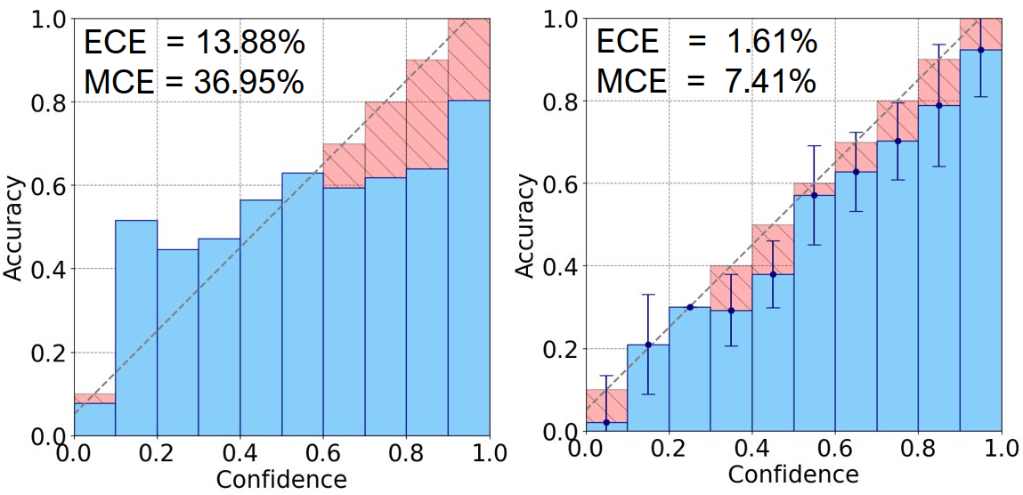
Figure 5: Calibration of a monolithic predictor (CNN, csp.) for racing car with horizon $k=100$. Left: uncalibrated, right: calibrated w/ isotonic regression and conformal bounds for $\alpha=0.05$.

An example reliability diagram (Fig. 5), shows a common trend we witnessed among uncalibrated chance predictors: underconfident for the rejected class (below $0.5$), overconfident for the chosen class (above $0.5$). More results are shown in Tab. 1 and  2. We can see that our calibration reduces the overconfidence and leads to a lower ECE — even for long prediction horizons, as per Tab. 1 and 2. The most effective calibrators were the isotonic regression for the racing car and ENIR for the cart pole. Furthermore, our calibrated predictive intervals are well-aligned with the calibration uncertainty. This leads us to conclude that safety chance prediction is a more suitable formulation for highly uncertain image-controlled autonomous systems.

Comparison 5: conformal calibration coverage

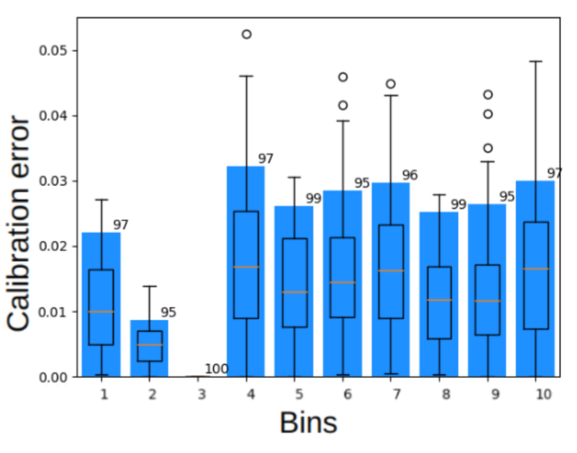
Figure 6: Our conformal bounds of monolithic predictor (CNN, csp.) for cart pole with horizon $k=18$ for $\alpha=0.05$ (blue) contain more than 95% of the true calibration errors (box and whisker plots).

Supporting our theoretical claims, the predicted intervals for calibration errors contained the true error values from the test data (Fig.  6). The sizes of these intervals are in Tab. 3 and  4, where the coverage of racing car is $97.74\%\pm 3.46\%$ and cart pole is $95.91\%\pm 6.65\%$. Our average error bound is $0.0924\pm 0.0438$ for the racing car and $0.0409\pm 0.0200$ for the cartpole. Therefore, our predicted chance $\pm$ its bin’s calibration bound can be used reliably and informatively online.

Table 1: ECE for the racing car: before (white rows) and after (gray rows), for horizons 20 to 200 with selected calibrators by hyperparameter- tuning.

Predictor	Model	$k=20$	$k=40$	$k=60$	$k=80$	$k=100$	$k=120$	$k=140$	$k=160$	$k=180$	$k=200$
mono. csp.	lat-LSTM	.0252$\pm$.0443	.0713$\pm$.0759	.1133$\pm$.0872	.1539$\pm$.1143	.1865$\pm$.1270	.1996$\pm$.1320	.1982$\pm$.1245	.2163$\pm$.1254	.2246$\pm$.1363	.2506$\pm$.1363
mono. csp.	lat-LSTM	.0030$\pm$.0056	.0069$\pm$.0063	.0109$\pm$.0134	.0099$\pm$.0102	.0125$\pm$.0157	.0118$\pm$.0147	.0141$\pm$.0107	.0146$\pm$.0117	.0153$\pm$.0145	.0179$\pm$.0113
mono. ind.	lat-LSTM	.0230$\pm$.0418	.0675$\pm$.0893	.1197$\pm$.0968	.1523$\pm$.1068	.1608$\pm$.1142	.1868$\pm$.1318	.1592$\pm$.1191	.1592$\pm$.1099	.1675$\pm$.1226	.1609$\pm$.1170
mono. ind.	lat-LSTM	.0021$\pm$.0051	.0054$\pm$.0095	.0054$\pm$.0081	.0070$\pm$.0081	.0074$\pm$.0069	.0100$\pm$.0105	.0141$\pm$.0129	.0125$\pm$.0121	.0119$\pm$.0096	.0127$\pm$.0098
mono. csp.	CNN	.0361$\pm$.0759	.0511$\pm$.0790	.0753$\pm$.0822	.0754$\pm$.0872	.1162$\pm$.0838	.1225$\pm$.1016	.1287$\pm$.1095	.1659$\pm$.0983	.1513$\pm$.0897	.1506$\pm$.1098
mono. csp.	CNN	.0025$\pm$.0047	.0037$\pm$.0054	.0078$\pm$.0072	.0061$\pm$.0100	.0119$\pm$.0134	.0067$\pm$.0077	.0122$\pm$.0108	.0140$\pm$.0148	.0107$\pm$.0072	.0121$\pm$.0123
mono. ind.	CNN	.0311$\pm$.0755	.0465$\pm$.0919	.0715$\pm$.0973	.0832$\pm$.0982	.1034$\pm$.0941	.1349$\pm$.1021	.1262$\pm$.1125	.1403$\pm$.1082	.1390$\pm$.1129	.1704$\pm$.1238
mono. ind.	CNN	.0037$\pm$.0083	.0028$\pm$.0060	.0079$\pm$.0099	.0076$\pm$.0109	.0054$\pm$.0069	.0094$\pm$.0093	.0096$\pm$.0092	.0109$\pm$.0137	.0090$\pm$.0097	.0137$\pm$.0127
comp. csp.	lat-LSTM	.0017$\pm$.0045	.0045$\pm$.0136	.0040$\pm$.0125	.0079$\pm$.0237	.0048$\pm$.0164	.0040$\pm$.0175	.0068$\pm$.0273	.0091$\pm$.0337	.0064$\pm$.0218	.0103$\pm$.0386
comp. csp.	lat-LSTM	.0005$\pm$.0011	.0011$\pm$.0039	.0007$\pm$.0027	.0010$\pm$.0042	.0010$\pm$.0051	.0009$\pm$.0034	.0010$\pm$.0036	.0009$\pm$.0037	.0011$\pm$.0036	.0010$\pm$.0031
comp. ind.	lat-LSTM	.0046$\pm$.0179	.0020$\pm$.0073	.0052$\pm$.0270	.0055$\pm$.0285	.0011$\pm$.0036	.0012$\pm$.0052	.0016$\pm$.0051	.0015$\pm$.0053	.0039$\pm$.0127	.0036$\pm$.0128
comp. ind.	lat-LSTM	.0006$\pm$.0018	.0006$\pm$.0024	.0002$\pm$.0008	.0002$\pm$.0007	.0001$\pm$.0005	.0002$\pm$.0006	.0007$\pm$.0022	.0004$\pm$.0012	.0007$\pm$.0022	.0008$\pm$.0035

Table 2: ECE for the cartpole: before (white rows) and after (gray rows), for horizons from 3 to 27 with selected calibrators by hyperparameter- tuning.

Predictor	Model	$k=3$	$k=6$	$k=9$	$k=12$	$k=15$	$k=18$	$k=21$	$k=24$	$k=27$
mono. csp.	lat-LSTM	.0042$\pm$.0107	.0034$\pm$.0079	.0033$\pm$.0115	.0018$\pm$.0038	.0024$\pm$.0049	.0098$\pm$.0213	.0474$\pm$.1037	.0760$\pm$.1662	.1600$\pm$.2061
mono. csp.	lat-LSTM	.0007$\pm$.0011	.0005$\pm$.0007	.0009$\pm$.0033	.0008$\pm$.0017	.0010$\pm$.0016	.0014$\pm$.0028	.0031$\pm$.0060	.0021$\pm$.0032	.0073$\pm$.0075
mono. ind.	lat-LSTM	.0035$\pm$.0117	.0043$\pm$.0110	.0019$\pm$.0043	.0020$\pm$.0037	.0028$\pm$.0065	.0096$\pm$.0225	.0506$\pm$.1082	.0776$\pm$.1688	.1627$\pm$.2068
mono. ind.	lat-LSTM	.0007$\pm$.0015	.0010$\pm$.0023	.0006$\pm$.0009	.0006$\pm$.0010	.0009$\pm$.0017	.0012$\pm$.0022	.0031$\pm$.0065	.0039$\pm$.0106	.0075$\pm$.0094
mono. csp.	CNN	.4919$\pm$.4892	.4915$\pm$.4886	.4928$\pm$.4883	.4919$\pm$.4847	.4923$\pm$.4730	.4930$\pm$.4431	.4942$\pm$.4003	.4919$\pm$.3652	.4915$\pm$.3398
mono. csp.	CNN	.0009$\pm$.0023	.0012$\pm$.0028	.0012$\pm$.0026	.0011$\pm$.0022	.0020$\pm$.0038	.0049$\pm$.0067	.0056$\pm$.0078	.0083$\pm$.0098	.0062$\pm$.0071
mono. ind.	CNN	.4933$\pm$.4842	.4923$\pm$.4859	.4917$\pm$.4841	.4924$\pm$.4856	.4916$\pm$.4720	.4926$\pm$.4428	.4918$\pm$.3994	.4928$\pm$.3653	.4916$\pm$.3398
mono. ind.	CNN	.0018$\pm$.0031	.0012$\pm$.0021	.0006$\pm$.0012	.0015$\pm$.0033	.0018$\pm$.0032	.0047$\pm$.0075	.0058$\pm$.0093	.0077$\pm$.0083	.0085$\pm$.0083
comp. csp.	lat-LSTM	.0389$\pm$.0619	.0631$\pm$.0651	.1029$\pm$.0964	.1378$\pm$.1626	.1548$\pm$.1877	.1492$\pm$.1637	.1773$\pm$.1708	.2140$\pm$.1891	.2197$\pm$.2068
comp. csp.	lat-LSTM	.0032$\pm$.0035	.0044$\pm$.0057	.0090$\pm$.0117	.0068$\pm$.0074	.0118$\pm$.0125	.0106$\pm$.0115	.0114$\pm$.0096	.0123$\pm$.0145	.0122$\pm$.0125
comp. ind.	lat-LSTM	.0414$\pm$.0684	.0547$\pm$.0888	.0751$\pm$.0962	.0730$\pm$.0646	.0788$\pm$.0613	.1003$\pm$.0837	.1342$\pm$.1128	.1492$\pm$.1277	.2116$\pm$.1558
comp. ind.	lat-LSTM	.0049$\pm$.0106	.0039$\pm$.0065	.0045$\pm$.0090	.0077$\pm$.0085	.0076$\pm$.0078	.0088$\pm$.0079	.0092$\pm$.0077	.0102$\pm$.0099	.0119$\pm$.0107

Table 3: Widths of conformal intervals for the racing car.

Predictor	Model	$k=20$	$k=40$	$k=60$	$k=80$	$k=100$	$k=120$	$k=140$	$k=160$	$k=180$	$k=200$
mono. csp.	lat-LSTM	.0051$\pm$.0042	.0232$\pm$.0270	.0249$\pm$.0391	.0222$\pm$.0187	.0194$\pm$.0156	.0178$\pm$.0187	.0187$\pm$.0110	.0194$\pm$.0231	.0187$\pm$.0099	.0169$\pm$.0100
mono. ind.	lat-LSTM	.0034$\pm$.0034	.0190$\pm$.0199	.0137$\pm$.0130	.0149$\pm$.0099	.0120$\pm$.0100	.0137$\pm$.0100	.0141$\pm$.0085	.0137$\pm$.0099	.0133$\pm$.0090	.0148$\pm$.0100
mono. csp.	CNN	.0079$\pm$.0075	.0267$\pm$.0283	.0261$\pm$.0334	.0118$\pm$.0115	.0169$\pm$.0177	.0129$\pm$.0108	.0147$\pm$.0086	.0138$\pm$.0101	.0136$\pm$.0108	.0168$\pm$.0104
mono. ind.	CNN	.0086$\pm$.0072	.0114$\pm$.0169	.0118$\pm$.0386	.0253$\pm$.0284	.0113$\pm$.0063	.0349$\pm$.0391	.0223$\pm$.0188	.0146$\pm$.0094	.0174$\pm$.0105	.0118$\pm$.0058
comp. csp.	lat-LSTM	.0299$\pm$.0147	.1360$\pm$.0572	.2162$\pm$.0793	.2659$\pm$.0896	.2939$\pm$.1012	.3183$\pm$.1095	.3397$\pm$.1178	.3554$\pm$.1223	.3841$\pm$.1320	.4126$\pm$.1420
comp. ind.	lat-LSTM	.0313$\pm$.0160	.1079$\pm$.0500	.1321$\pm$.0616	.1623$\pm$.0680	.2060$\pm$.0869	.2393$\pm$.1034	.2730$\pm$.1170	.3047$\pm$.1339	.3279$\pm$.1350	.3610$\pm$.1395

Table 4: Widths of conformal intervals for the cartpole.

Predictor	Model	$k=3$	$k=6$	$k=9$	$k=12$	$k=15$	$k=18$	$k=21$	$k=24$	$k=27$
mono. csp.	lat-LSTM	.0064$\pm$.0088	.0059$\pm$.0082	.0061$\pm$.0065	.0069$\pm$.0092	.0097$\pm$.0093	.0226$\pm$.0180	.0581$\pm$.0486	.1270$\pm$.0922	.0962$\pm$.0850
mono. ind.	lat-LSTM	.0077$\pm$.0094	.0059$\pm$.0095	.0038$\pm$.0062	.0074$\pm$.0092	.0127$\pm$.0129	.0234$\pm$.0171	.0573$\pm$.0472	.1258$\pm$.0911	.0989$\pm$.0858
mono. csp.	CNN	.0055$\pm$.0081	.0049$\pm$.0088	.0074$\pm$.0127	.0097$\pm$.0170	.0200$\pm$.0235	.0347$\pm$.0310	.0449$\pm$.0298	.0599$\pm$.0319	.0694$\pm$.0273
mono. ind.	CNN	.0134$\pm$.0123	.0102$\pm$.0127	.0106$\pm$.0168	.0091$\pm$.0139	.0190$\pm$.0211	.0330$\pm$.0283	.0470$\pm$.0311	.0588$\pm$.0295	.0676$\pm$.0258
comp. csp.	lat-LSTM	.0275$\pm$.0243	.0464$\pm$.0312	.0525$\pm$.0324	.0584$\pm$.0340	.0579$\pm$.0319	.0625$\pm$.0282	.0721$\pm$.0298	.0734$\pm$.0233	.0754$\pm$.0263
comp. ind.	lat-LSTM	.0249$\pm$.0248	.0306$\pm$.0304	.0426$\pm$.0325	.0500$\pm$.0291	.0536$\pm$.0301	.0601$\pm$.0312	.0647$\pm$.0262	.0678$\pm$.0285	.0803$\pm$.0273

5 Related Work

Performance and safety evaluation for autonomy

A variety of recent research enables autonomous systems to self-evaluate their competency (Basich et al. 2022). Performance metrics vary significantly and include such examples as the time to navigate to a goal location or whether a safety constraint was violated, which is the focus of our paper. For systems that have access to their low-dimensional state, such as the velocity and the distance from the goal, hand-crafted indicators have been successful in measuring performance degradation. These indicators have been referred to robot vitals (Ramesh, Stolkin, and Chiou 2022), alignment checkers (Gautam et al. 2022), assumption monitors (Ruchkin et al. 2022), and operator trust (Conlon, Szafir, and Ahmed 2022). Typically, these indicators rely on domain knowledge and careful offline analysis of the system, which are difficult to obtain and perform for high-dimensional systems.

Autonomy with deep neural network (DNN) controllers is vulnerable to distribution shift (Moreno-Torres et al. 2012; Huang et al. 2020) and difficult to analyze. On the model-based side, a number of closed-loop verification approaches perform analyze reachability and safety of a DNN-controlled system (Ivanov et al. 2021; Tran, Xiang, and Johnson 2022), but when applied to vision-based systems, require detailed modeling of the vision subsystem and have limited scalability (Santa Cruz and Shoukry 2022; Hsieh et al. 2022). On the other hand, model-free safety predictions rely on the correlation between performance and uncertainty measures/anomaly scores, such as autoencoder reconstruction errors (Stocco et al. 2020) and distances to representative training data (Yang et al. 2022); however, these approaches fail to fully utilize the information about the system’s closed-loop nature. Striking the balance between model-based and model-free approaches are black-box statistical methods for risk assessment and safety verification (Cleaveland et al. 2022; Zarei, Wang, and Pajic 2020; Qin et al. 2022; Michelmore et al. 2020). They usually require low-dimensional states and rich outcome labels (such as signal robustness) — an assumption that we are relaxing in this work while addressing a similar problem.

Trajectory prediction

A common way of predicting the system’s performance and safety is by inferring it from predicted trajectories. Classic approaches consider model-based prediction (Lefèvre, Vasquez, and Laugier 2014), for instance, estimating collision risk with bicycle dynamics and Kalman filtering (Ammoun and Nashashibi 2009). One common approach with safety guarantees is Hamilton-Jacobi (HJ) reachability (Li et al. 2021; Nakamura and Bansal 2023), which requires precomputation based on a dynamical model. Among many deep learning-based predictors (Huang et al. 2022), a recently popular architecture is Trajectron++ (Salzmann et al. 2020) takes in high-dimensional scene graphs and outputs future trajectories for multiple agents. A conditional VAE (Sohn, Lee, and Yan 2015) is adopted in Trajectron++ to add constraints at the decoding stage. Learning-based trajectory predictions can be augmented with conformal prediction to improve their reliability (Lindemann et al. 2023; Muthali et al. 2023). In comparison, our work eschews handcrafted scene and state representations, instead using image and latent representations that are informed by safety.

Safe control

Safe planning and control solve a problem complementary to ours: controlling a system safely, usually with respect to a dynamical model, such as motion planning under uncertainty for uncertain systems (Knuth et al. 2021; Hibbard et al. 2022; Chou and Tedrake 2023) and a growing body of work on control barrier functions (Ames et al. 2019; Xiao, Cassandras, and Belta 2023). Some recent approaches are robust to measurement errors induced by learning-based perception (Dean et al. 2021; Yang et al. 2023), but at their core, they still hinge on the utilization of low-dimensional states, a paradigm we aim to circumvent entirely. Importantly, one of our constraints is assuming the existence of an end-to-end controller (possibly implemented with the above methods), with no room for modifications.

Confidence calibration

The softmax scores of classification neural networks can be interpreted as probabilities for each class; however, standard training leads to miscalibrated neural networks (Guo et al. 2017; Minderer et al. 2021), as measured by Brier score and Expected Calibration Error (ECE). Calibration approaches can be categorized into extrinsic (post-hoc) calibration added on top of a trained network, such as Platt and temperature scaling (Platt 1999; Guo et al. 2017), isotonic regression (Zadrozny and Elkan 2002), and histogram/Bayesian binning (Naeini, Cooper, and Hauskrecht 2015) — and intrinsic calibration to modify the training, such as ensembles (Zhang, Kailkhura, and Han 2020), adversarial training (Lee et al. 2018), and learning from hints (DeVries and Taylor 2018), error distances (Xing et al. 2019), or true class probabilities (Corbiere et al. 2019). Similar techniques have been developed for calibrated regression (Vovk et al. 2020; Marx et al. 2022). It is feasible to obtain calibration guarantees for safety chance predictions (Ruchkin et al. 2022; Cleaveland et al. 2023), but it requires a low-dimensional model-based setting. To the authors’ best knowledge, such guarantees have not been instantiated in a model-free autonomy setting.

Deep surrogate models

For systems with high-resolution images and complex dynamical models, trajectory predictions become particularly challenging. Physics-based methods and classical machine learning methods may not be applicable to these tasks, leading to the almost exclusive application of deep learning for prediction. Sequence prediction models, which originate in deep video prediction (Oprea et al. 2022), usually do not perform well since they require long horizons and a large number of samples from each controller. However, incorporating additional information, such as states, observations, and actions, in sequence predictions can improve their performance (Strickland, Fainekos, and Amor 2018), and our predictors take advantage of that.

High-dimensional sensor data contains substantial redundant and irrelevant information, which leads to higher computational costs. Generative adversarial networks (GANs) map the observations into low-dimensional latent space, which can enable conventional assurance tools (Katz et al. 2021). Low-dimensional representations can incorporate conformal predictions to monitor the real-time performance (Boursinos and Koutsoukos 2021). World models (Ha and Schmidhuber 2018) are used as a surrogate method of training a controller instead of using reinforcement learning (RL). They achieve better results to train the controllers than the basic reinforcement learning method. This kind of model can learn how the dynamical system works, which collects random observations and actions as inputs and outputs the future states. Then it uses a VAE to compress observations into a latent space (low-dimensional vectors) and trains a mixed-density recurrent neural network (MDN-RNN) to forecast the next-step latent observations. The decoder of the VAE maps the latent vector into observation space. This model is adopted to do trajectory predictions and get the competency assessment through the forecasting trajectory (Acharya, Russell, and Ahmed 2022). The original world model uses a VAE to compress the observations and an MDN-RNN to perform sequence prediction. Lately, more advanced models like DreamerV2 (Hafner et al. 2022) and IRIS (Micheli, Alonso, and Fleuret 2023) adopt recent deep computer vision models like vision transformers to achieve more vivid images. The trajectory predicted by world models can also provide uncertainty measurement for agents (Acharya, Russell, and Ahmed 2023). In our method, we adopt the architecture of the initial version of world models which have VAE and recurrent models and compare them with other deep learning models like the recurrent network alone and convolutional recurrent networks. On top of these approaches, we have developed chance calibration guarantees, which were previously unexplored.

6 Discussion and Conclusion

Limitations: our predictor family’s scope is limited to systems where safety can be inferred from raw sensor data. Also, our safety evaluators are system-specific, and developing them may require substantial effort; however, this effort is balanced with the savings of not needing to design state representations and develop dynamical models (both of which would be system-specific as well).

Some approaches have performed poorly (not reported due to space limits). One such approach is flexible-horizon predictors, which output the time to the first expected safety violation. Their prediction space appeared too complex and insufficiently regularized, leading to poor performance. Also, latent space evaluators (as opposed to image evaluators) have shown particularly poor performance, which indicates that the latent state vectors failed to preserve safety information. Thus, learning strong safety-informed representations for autonomy remains an open problem. Though quantized latent expression now is used for video predictions  (Walker, Razavi, and Oord 2021) and video generation (Yan et al. 2021), the CLIP (Radford et al. 2021), a multimodal unsupervised method, unifies the representations of images and texts. With the rise of large language models, meaning representations in multimodal autoregressive models (Liu et al. 2023) may provide more possibilities to explore the surrogate dynamics of autonomy systems.

Future work includes adding physical constraints to latent states similar to Neural ODEs (Wen, Wang, and Metaxas 2022), jointly learning forecasters and evaluators to overcome distribution shifts, using world-model transformer architectures, and applying predictors to physical systems.

7 Acknowledgments

We would like to thank Kaleb Smith (NVIDIA AI Technology Center), Yuang Geng (University of Florida), and anonymous reviewers for their insightful feedback on this research.

Appendix

A  Hyperparameters

We used Pytorch 1.13.1 with the Adam optimizer. The maximum training epoch is 500 for VAEs and 100 for predictors. The starting learning rate of $10^{-3}$, and the reduction factor of 0.1 with a patience of 5 epochs. The early-stopping patience is 15 epochs. The batch size of the classifier, the latent predictor, and the image predictor are 128, 64, and 16. The architecture for the evaluator and monolithic single-image predictor consists of 2 convolutional layers with kernel sizes of 3 and 5 respectively, 3 linear layers and 1 softmax layer. Each 2D convolution layer is combined with max-pooling layers with the size of 2*2 with stride 2. For the VAE, the latent size is 32. The encoder has 4 convolutional layers and 2 linear layers. Each convolutional layer is combined with a ReLU, and the decoder has a similar structure with transposed convolutional layers. The structure of the monolithic sequence predictor and the composite latent predictor is one LSTM layer and one linear layer. The monolithic predictor has an extra softmax layer, and has an output size of 2, while the composite has an output size of 32. The safety loss uses $\lambda_{1}=1$ and $\lambda_{2}=4096$, which equals the total pixel count in our images. The miscoverage level is $\alpha=0.05$.

The following tables contain the hyperparameters:

• The dataset size and prediction horizons are shown (Tab. 11)

• The architecture of our evaluator and single-image predictors (Tab. 13)

• The architecture of our image forecaster (Tab. 14)

• The architecture of our latent LSTM, which uses an encoder to compress images (Tab. 15)

• The architecture of our latent forecaster (Tab. 16)

• The architecture of our VAEs (Tab. 17)

B  Result Tables

Table 5: Predictors’ F1 scores for the racing car.

Predictor	Model	$k=20$	$k=40$	$k=60$	$k=80$	$k=100$	$k=120$	$k=140$	$k=160$	$k=180$	$k=200$
mon. csp.	lat-LSTM	96.7 $\pm$ 0.5	93.1 $\pm$ 1.2	87.8 $\pm$ 2.2	83.4 $\pm$ 2.6	80.9 $\pm$ 3.0	79.2 $\pm$ 2.5	77.5 $\pm$ 2.1	75.5 $\pm$ 2.8	74.9 $\pm$ 6.0	72.3 $\pm$ 3.1
mon. ind.	lat-LSTM	96.6 $\pm$ 0.6	89.9 $\pm$ 2.1	86.2 $\pm$ 2.9	82.4 $\pm$ 4.8	80.8 $\pm$ 4.7	78.9 $\pm$ 5.5	77.6 $\pm$ 5.1	72.9 $\pm$ 8.9	70.7 $\pm$ 5.6	69.7 $\pm$ 6.1
mon. csp.	CNN	92.3 $\pm$ 1.6	87.3 $\pm$ 3.7	83.3 $\pm$ 5.3	80.9 $\pm$ 3.4	78.4 $\pm$ 10.6	77.3 $\pm$ 5.2	75.5 $\pm$ 2.6	74.0 $\pm$ 10.9	71.4 $\pm$ 6.9	72.0 $\pm$ 9.2
mon. ind.	CNN	92.6 $\pm$ 1.6	87.9 $\pm$ 2.8	82.4 $\pm$ 4.8	78.9 $\pm$ 5.8	77.6 $\pm$ 5.1	72.9 $\pm$ 8.9	70.7 $\pm$ 5.6	69.7 $\pm$ 6.1	69.1 $\pm$ 5.8	68.6 $\pm$ 5.3
comp. csp.	lat-LSTM e	92.8 $\pm$ 0.5	84.5 $\pm$ 1.7	74.9 $\pm$ 7.7	66.1 $\pm$ 12.0	52.9 $\pm$ 17.7	47.3 $\pm$ 20.8	43.7 $\pm$ 21.6	41.8$\pm$21.7	38.0 $\pm$ 23.8	35.9 $\pm$ 25.8
comp. csp.	lat-LSTM v	93.5 $\pm$ 0.8	86.6 $\pm$ 0.4	80.9 $\pm$ 1.6	75.8 $\pm$ 4.8	71.6 $\pm$ 8.1	69.8 $\pm$ 8.0	67.4 $\pm$ 6.3	66.1 $\pm$ 6.0	63.6 $\pm$ 4.7	60.2 $\pm$ 3.5
comp. ind.	lat-LSTM e	94.5 $\pm$ 0.1	83.7 $\pm$ 3.3	68.9 $\pm$ 12.1	67.0 $\pm$ 11.8	63.3 $\pm$ 13.9	61.3 $\pm$ 15.7	59.2 $\pm$ 16.4	56.3 $\pm$ 17.2	54.2 $\pm$ 17.0	51.9 $\pm$ 16.5
comp. ind.	lat-LSTM v	93.4 $\pm$ 0.5	83.9 $\pm$ 2.1	74.3 $\pm$ 6.9	70.6 $\pm$ 8.9	71.9 $\pm$ 4.3	68.5 $\pm$ 7.0	64.6 $\pm$ 10.5	62.8 $\pm$ 9.4	59.9 $\pm$ 10.7	56.3 $\pm$ 10.6
comp. csp	conv-LSTM e	6.7 $\pm$ 1.9	6.8 $\pm$ 1.8	6.7 $\pm$ 1.6	6.6 $\pm$ 1.5	6.4 $\pm$ 1.6	6.3 $\pm$ 1.7	6.2 $\pm$ 1.8	6.0 $\pm$ 1.6	5.7 $\pm$ 1.3	4.9 $\pm$ 0.8
comp. csp	conv-LSTM v1	37.8 $\pm$ 27.6	37.1 $\pm$ 26.6	36.3 $\pm$ 25.6	35.8 $\pm$ 24.9	35.3 $\pm$ 24.3	34.7 $\pm$ 23.9	34.2 $\pm$ 22.9	33.6 $\pm$ 22.3	33.3 $\pm$ 21.9	32.2 $\pm$ 20.9
comp. csp	conv-LSTM v2	4.4 $\pm$ 2.6	4.3 $\pm$ 2.4	4.2 $\pm$ 2.2	4.1 $\pm$ 2.2	4.0 $\pm$ 2.1	3.9 $\pm$ 2.0	3.9 $\pm$ 1.9	3.8 $\pm$ 1.9	3.8 $\pm$ 1.9	3.7 $\pm$ 1.6

Table 6: Predictors’ FPRs for the racing car.

Predictor	Model	$k=20$	$k=40$	$k=60$	$k=80$	$k=100$	$k=120$	$k=140$	$k=160$	$k=180$	$k=200$
mon. csp.	lat-LSTM	3.4 $\pm$ 0.6	8.6 $\pm$ 2.1	17.7 $\pm$ 3.5	25.2 $\pm$ 5.8	30.4 $\pm$ 5.1	33.9 $\pm$ 6.4	38.4 $\pm$ 6.5	38.2 $\pm$ 5.6	37.3 $\pm$ 11.7	37.8 $\pm$ 7.4
mon. ind.	lat-LSTM	4.2 $\pm$ 1.7	13.2 $\pm$ 5.6	22.0 $\pm$ 8.2	25.9 $\pm$ 9.4	34.4 $\pm$ 11.2	33.4 $\pm$ 8.4	32.5 $\pm$ 6.6	34.9 $\pm$ 7.1	31.8 $\pm$ 4.9	30.8 $\pm$ 4.1
mon. csp.	CNN	9.1 $\pm$ 1.6	17.4 $\pm$ 3.7	24.6$\pm$5.3	32.2 $\pm$ 3.4	36.9 $\pm$ 10.6	36.3 $\pm$ 5.2	38.8 $\pm$ 2.6	39.0 $\pm$ 2.2	43.7 $\pm$ 9.4	40.4 $\pm$ 9.2
mon. ind.	CNN	9.6 $\pm$ 4.2	16.5 $\pm$ 7.2	25.9 $\pm$ 9.2	29.6 $\pm$ 10.4	31.3 $\pm$ 9.9	33.4 $\pm$ 8.4	32.5 $\pm$ 6.6	34.9 $\pm$ 7.1	31.8 $\pm$ 4.9	27.8 $\pm$ 4.1
comp. csp.	lat-LSTM e	11.1 $\pm$ 4.7	23.0 $\pm$ 9.4	29.7 $\pm$ 12.8	28.9 $\pm$ 11.6	22.8 $\pm$ 10.8	21.0 $\pm$ 13.4	20.3 $\pm$ 15.6	19.8 $\pm$ 17.8	18.7 $\pm$ 21.3	18.2 $\pm$ 21.3
comp. csp.	lat-LSTM v	45.0 $\pm$ 17.0	76.5 $\pm$ 14.4	84.8 $\pm$ 10.3	84.9 $\pm$ 11.4	82.7 $\pm$ 13.6	84.0 $\pm$ 13.0	84.7 $\pm$ 12.5	85.3 $\pm$ 12.2	86.3 $\pm$ 10.3	87.7 $\pm$ 10.5
comp. ind.	lat-LSTM e	35.3 $\pm$ 17.1	64.2 $\pm$ 17.1	72.7$\pm$15.6	73.6 $\pm$ 16.2	72.5 $\pm$ 16.8	72.4 $\pm$ 22.1	70.9 $\pm$ 27.1	69.3 $\pm$ 30.5	68.4 $\pm$ 33.3	68.3 $\pm$ 34.9
comp. ind.	lat-LSTM v	61.8 $\pm$ 18.8	78.2 $\pm$ 12.1	79.9 $\pm$ 11.3	79.2 $\pm$ 11.8	80.8 $\pm$ 11.2	79.0 $\pm$ 20.0	76.9 $\pm$ 21.0	77.5 $\pm$ 22.3	75.1 $\pm$ 25.9	75.7 $\pm$ 26.3
comp. csp	conv-LSTM e	0.6 $\pm$ 0.5	1.1 $\pm$ 0.9	1.4 $\pm$ 1.1	1.7 $\pm$ 1.1	1.9$\pm$ 1.2	2.0 $\pm$ 1.2	2.2 $\pm$ 1.1	2.4 $\pm$ 1.2	2.6 $\pm$ 1.4	3.0 $\pm$ 1.5
comp. csp	conv-LSTM v1	16.2 $\pm$ 10.3	19.9 $\pm$ 13.7	23.4 $\pm$ 16.0	28.4 $\pm$ 17.1	32.2 $\pm$ 17.7	37.4 $\pm$ 18.3	43.2 $\pm$ 19.3	47.8 $\pm$ 19.5	11.0 $\pm$ 7.9	26.1 $\pm$ 16.6
comp. csp	conv-LSTM v2	1.1 $\pm$ 0.4	1.4 $\pm$ 0.8	1.6 $\pm$ 1.0	1.9 $\pm$ 1.1	1.8 $\pm$ 1.1	1.9 $\pm$ 1.1	2.0 $\pm$ 1.2	2.0 $\pm$ 1.2	2.2 $\pm$ 1.4	2.2 $\pm$ 1.4

Table 7: Predictors’ F1 scores for the cartpole.

Predictor	Model	$k=3$	$k=6$	$k=9$	$k=12$	$k=15$	$k=18$	$k=21$	$k=24$	$k=27$
mono. csp.	lat-LSTM	99.8 $\pm$ 0.1	99.8 $\pm$ 0.1	99.6 $\pm$ 0.2	99.5 $\pm$ 0.2	99.4 $\pm$ 0.3	99.3 $\pm$ 0.3	98.4 $\pm$ 0.8	93.4 $\pm$ 6.7	86.7 $\pm$ 13.9
mono. ind.	lat-LSTM	99.8 $\pm$ 0.0	99.8 $\pm$ 0.0	99.8 $\pm$ 0.0	99.8 $\pm$ 0.0	99.5 $\pm$ 0.1	98.7 $\pm$ 0.7	93.8 $\pm$ 6.4	88.1 $\pm$ 12.2	85.3 $\pm$ 13.4
mono. sp.	CNN	99.8 $\pm$ 0.1	99.8 $\pm$ 0.1	99.7 $\pm$ 0.1	99.4 $\pm$ 0.1	98.3 $\pm$ 1.1	94.8 $\pm$ 5.4	90.6 $\pm$ 9.7	85.4 $\pm$ 15.4	81.8 $\pm$ 18.6
mono. ind.	CNN	99.5 $\pm$ 0.2	99.6 $\pm$ 0.2	99.5 $\pm$ 0.1	99.3 $\pm$ 0.1	98.3 $\pm$ 0.7	94.8 $\pm$ 4.5	90.6 $\pm$ 8.3	86.9 $\pm$ 11.2	84.7 $\pm$ 12.1
comp. csp.	lat-LSTM e	92.9 $\pm$ 0.6	90.4 $\pm$ 4.3	60.5 $\pm$ 31.5	29.3 $\pm$ 40.5	43.3 $\pm$ 36.1	33.1 $\pm$ 23.5	22.2 $\pm$ 28.6	19.8 $\pm$ 26.9	21.9 $\pm$ 29.0
comp. csp.	lat-LSTM v	88.6 $\pm$ 4.4	85.5 $\pm$ 7.2	67.3 $\pm$ 12.1	29.9 $\pm$ 30.1	49.9 $\pm$ 34.2	55.8 $\pm$ 19.8	64.9 $\pm$ 8.5	64.1 $\pm$ 5.8	51.2 $\pm$ 13.7
comp. ind.	lat-LSTM e	94.8 $\pm$ 1.9	93.1 $\pm$ 3.7	83.7 $\pm$ 10.3	48.1 $\pm$ 25.7	40.4 $\pm$ 28.4	60.2 $\pm$ 10.6	66.2 $\pm$ 3.2	62.8 $\pm$ 5.4	62.6 $\pm$ 9.0
comp. ind.	lat-LSTM v	88.3 $\pm$ 4.1	87.1 $\pm$ 6.4	83.9 $\pm$ 9.7	61.9 $\pm$ 24.2	52.5 $\pm$ 22.9	68.6 $\pm$ 8.4	76.4 $\pm$ 3.1	73.4 $\pm$ 1.6	70.5 $\pm$ 2.0
comp. ind.	conv-LSTM e	64.0 $\pm$ 1.8	0.0 $\pm$ 0.0	0.0 $\pm$ 0.0	0.0 $\pm$ 0.0	0.0 $\pm$ 0.0	0.0 $\pm$ 0.0	0.0 $\pm$ 0.0	0.0 $\pm$ 0.0	0.0 $\pm$ 0.0
comp. ind.	conv-LSTM v	67.3 $\pm$ 2.9	0.0 $\pm$ 0.0	0.0 $\pm$ 0.0	0.0 $\pm$ 0.0	0.0 $\pm$ 0.0	0.0 $\pm$ 0.0	0.0 $\pm$ 0.0	0.0 $\pm$ 0.0	0.0 $\pm$ 0.0

Table 8: Predictors’ FPR for the cart pole.

Predictor	Model	$k=3$	$k=6$	$k=9$	$k=12$	$k=15$	$k=18$	$k=21$	$k=24$	$k=27$
mono. csp.	lat-LSTM	0.1 $\pm$ 0.0	0.2 $\pm$ 0.1	0.5 $\pm$ 0.5	0.6 $\pm$ 0.4	0.7 $\pm$ 0.5	0.8 $\pm$ 0.5	2.5 $\pm$ 1.8	9.3 $\pm$ 8.8	20.8 $\pm$ 20.4
mono. ind.	lat-LSTM	0.4 $\pm$ 0.1	0.3 $\pm$ 0.1	0.2 $\pm$ 0.1	0.3 $\pm$ 0.0	0.3 $\pm$ 0.2	0.3 $\pm$ 0.2	0.4 $\pm$ 0.2	0.4 $\pm$ 0.3	1.2 $\pm$ 0.8
mono. csp.	CNN	0.0 $\pm$ 0.0	0.0 $\pm$ 0.0	0.0 $\pm$ 0.0	0.0 $\pm$ 0.0	2.7 $\pm$ 2.6	10.8 $\pm$ 11.4	16.3 $\pm$ 17.1	17.3 $\pm$ 15.1	19.3 $\pm$ 13.6
mono. ind.	CNN	0.4 $\pm$ 0.1	0.4 $\pm$ 0.1	0.4 $\pm$ 0.1	0.6 $\pm$ 0.2	1.1 $\pm$ 0.5	0.9 $\pm$ 0.7	0.8 $\pm$ 0.6	0.8 $\pm$ 0.5	1.0 $\pm$ 0.3
comp. csp.	lat-LSTM e	9.3 $\pm$ 0.5	17.0 $\pm$ 4.0	22.1 $\pm$ 4.9	26.3 $\pm$ 11.0	23.1 $\pm$ 8.0	22.8 $\pm$ 6.4	30.9 $\pm$ 9.4	36.2 $\pm$ 12.7	36.1 $\pm$ 12.2
comp. csp.	lat-LSTM v	28.1 $\pm$ 3.7	40.0 $\pm$ 2.7	50.0 $\pm$ 13.7	50.6 $\pm$ 20.9	42.0 $\pm$ 29.4	41.2 $\pm$ 20.0	56.0 $\pm$ 13.1	64.9 $\pm$ 13.4	63.6 $\pm$ 17.0
comp. ind.	lat-LSTM e	6.1 $\pm$ 4.3	9.8 $\pm$ 6.4	11.5 $\pm$ 7.6	11.3 $\pm$ 7.6	20.6 $\pm$ 0.8	32.3 $\pm$ 7.9	39.8 $\pm$ 15.1	39.4 $\pm$ 20.1	53.8 $\pm$ 25.2
comp. ind.	lat-LSTM v	34.9 $\pm$ 4.7	38.4 $\pm$ 2.3	38.1 $\pm$ 6.2	31.9 $\pm$ 4.1	32.3 $\pm$ 3.7	41.5 $\pm$ 8.0	53.1 $\pm$ 11.8	56.1 $\pm$ 1.7	67.7 $\pm$ 13.8
comp. csp	conv-LSTM e	100.0 $\pm$ 0.0	0.0 $\pm$ 0.0	0.0 $\pm$ 0.0	0.0 $\pm$ 0.0	0.0 $\pm$ 0.0	0.0 $\pm$ 0.0	0.0 $\pm$ 0.0	0.0 $\pm$ 0.0	0.0 $\pm$ 0.0
comp. csp	conv-LSTM v	100.0 $\pm$ 0.0	0.0 $\pm$ 0.0	0.0 $\pm$ 0.0	0.0 $\pm$ 0.0	0.0 $\pm$ 0.0	0.0 $\pm$ 0.0	0.0 $\pm$ 0.0	0.0 $\pm$ 0.0	0.0 $\pm$ 0.0

Table 9: Brier score comparison before (white rows) and after (gray rows) calibration for the racing car with selected calibrators by hyperparameter- tuning.

Predictor	Model	$k=20$	$k=40$	$k=60$	$k=80$	$k=100$	$k=120$	$k=140$	$k=160$	$k=180$	$k=200$
mono. csp.	lat-LSTM	.0327$\pm$.0509	.0977$\pm$.0715	.1435$\pm$.0973	.1796$\pm$.0950	.2013$\pm$.1191	.2192$\pm$.1264	.2328$\pm$.1150	.2409$\pm$.1161	.2492$\pm$.1284	.2689$\pm$.1307
mono. csp.	lat-LSTM	.0294$\pm$.0446	.0859$\pm$.0578	.1167$\pm$.0698	.1481$\pm$.0732	.1524$\pm$.0767	.1613$\pm$.0756	.1741$\pm$.0693	.1788$\pm$.0702	.1858$\pm$.0681	.1949$\pm$.0591
mono. ind.	lat-LSTM	.0268$\pm$.0466	.0924$\pm$.0978	.1391$\pm$.1050	.1669$\pm$.1086	.1882$\pm$.1142	.2066$\pm$.1246	.1940$\pm$.1174	.2173$\pm$.1273	.2130$\pm$.1168	.2146$\pm$.1181
mono. ind.	lat-LSTM	.0232$\pm$.0391	.0790$\pm$.0654	.1105$\pm$.0755	.1428$\pm$.0832	.1516$\pm$.0850	.1557$\pm$.0872	.1603$\pm$.0882	.1652$\pm$.0854	.1670$\pm$.0879	.1714$\pm$.0875
mono. csp.	CNN	.0315$\pm$.0496	.0938$\pm$.0992	.1276$\pm$.0974	.1644$\pm$.1083	.1771$\pm$.1083	.1870$\pm$.1067	.1945$\pm$.1019	.2028$\pm$.1022	.2137$\pm$.1082	.2451$\pm$.1328
mono. csp.	CNN	.0280$\pm$.0430	.0790$\pm$.0748	.1066$\pm$.0799	.1373$\pm$.0804	.1431$\pm$.0843	.1517$\pm$.0860	.1615$\pm$.0869	.1650$\pm$.0825	.1684$\pm$.0844	.1743$\pm$.0804
mono. ind.	CNN	.0359$\pm$.0545	.0931$\pm$.0832	.1361$\pm$.0944	.1874$\pm$.1028	.1924$\pm$.0988	.1982$\pm$.1111	.2067$\pm$.1038	.2047$\pm$.1011	.2106$\pm$.1114	.2218$\pm$.1040
mono. ind.	CNN	.0314$\pm$.0455	.0765$\pm$.0739	.1116$\pm$.0785	.1488$\pm$.0769	.1575$\pm$.0738	.1607$\pm$.0838	.1690$\pm$.0856	.1753$\pm$.0749	.1777$\pm$.0812	.1823$\pm$.0804
comp. csp.	lat-LSTM	.0341$\pm$.0134	.1465$\pm$.0368	.2303$\pm$.0509	.2966$\pm$.0567	.3139$\pm$.0636	.3408$\pm$.0651	.3626$\pm$.0701	.3778$\pm$.0720	.4099$\pm$.0782	.4402$\pm$.0836
comp. csp.	lat-LSTM	.0335$\pm$.0128	.1446$\pm$.0403	.2270$\pm$.0562	.2797$\pm$.0689	.3087$\pm$.0727	.3231$\pm$.0808	.3416$\pm$.0789	.3682$\pm$.0900	.3981$\pm$.0978	.4269$\pm$.1092
comp. ind.	lat-LSTM	.0368$\pm$.0158	.1157$\pm$.0424	.1681$\pm$.0576	.2158$\pm$.0691	.2539$\pm$.0782	.2922$\pm$.0883	.3267$\pm$.0981	.3518$\pm$.1078	.3752$\pm$.1081	.4079$\pm$.1162
comp. ind.	lat-LSTM	.0359$\pm$.0147	.1145$\pm$.0431	.1399$\pm$.0524	.1671$\pm$.0593	.2131$\pm$.0796	.2495$\pm$.0848	.2853$\pm$.0959	.3185$\pm$.1069	.3418$\pm$.1152	.3693$\pm$.1228

Table 10: Brier score comparison before (white rows) and after (gray rows) calibration for the cartpole with selected calibrators by hyperparameter- tuning.

Predictor	Model	$k=3$	$k=6$	$k=9$	$k=12$	$k=15$	$k=18$	$k=21$	$k=24$	$k=27$
mono. csp.	lat-LSTM	.0021$\pm$.0037	.0020$\pm$.0035	.0015$\pm$.0022	.0024$\pm$.0045	.0039$\pm$.0069	.0134$\pm$.0170	.0693$\pm$.0541	.1552$\pm$.0657	.1978$\pm$.0373
mono. csp.	lat-LSTM	.0021$\pm$.0038	.0019$\pm$.0034	.0015$\pm$.0022	.0023$\pm$.0042	.0037$\pm$.0063	.0126$\pm$.0155	.0550$\pm$.0403	.1211$\pm$.0624	.1270$\pm$.0567
mono. ind.	lat-LSTM	.0025$\pm$.0038	.0019$\pm$.0040	.0011$\pm$.0023	.0024$\pm$.0044	.0051$\pm$.0086	.0135$\pm$.0166	.0683$\pm$.0554	.1547$\pm$.0673	.2014$\pm$.0374
mono. ind.	lat-LSTM	.0025$\pm$.0036	.0019$\pm$.0038	.0011$\pm$.0022	.0024$\pm$.0044	.0048$\pm$.0077	.0127$\pm$.0153	.0539$\pm$.0407	.1191$\pm$.0612	.1285$\pm$.0588
mono. csp.	CNN	.4841$\pm$.4809	.4846$\pm$.4811	.4850$\pm$.4799	.4845$\pm$.4777	.4848$\pm$.4658	.4833$\pm$.4331	.4856$\pm$.3878	.4860$\pm$.3409	.4893$\pm$.2910
mono. csp.	CNN	.0029$\pm$.0053	.0030$\pm$.0059	.0045$\pm$.0088	.0059$\pm$.0117	.0182$\pm$.0276	.0467$\pm$.0455	.0783$\pm$.0579	.1068$\pm$.0615	.1228$\pm$.0380
mono. ind.	CNN	.4889$\pm$.4813	.4874$\pm$.4817	.4862$\pm$.4773	.4855$\pm$.4782	.4857$\pm$.4637	.4858$\pm$.4328	.4881$\pm$.3866	.4878$\pm$.3404	.4876$\pm$.2907
mono. ind.	CNN	.0066$\pm$.0088	.0060$\pm$.0097	.0079$\pm$.0149	.0059$\pm$.0112	.0157$\pm$.0213	.0474$\pm$.0440	.0794$\pm$.0579	.1039$\pm$.0532	.1269$\pm$.0446
comp. ind.	lat-LSTM	.0440$\pm$.0652	.0570$\pm$.0751	.0777$\pm$.0773	.0820$\pm$.0606	.0900$\pm$.0684	.1099$\pm$.0794	.1420$\pm$.0983	.1533$\pm$.1063	.2174$\pm$.1165
comp. ind.	lat-LSTM	.0327$\pm$.0436	.0435$\pm$.0518	.0638$\pm$.0588	.0698$\pm$.0505	.0763$\pm$.0544	.0912$\pm$.0608	.1060$\pm$.0599	.1109$\pm$.0590	.1428$\pm$.0580
comp. csp.	lat-LSTM	.0464$\pm$.0678	.0691$\pm$.0703	.1020$\pm$.0866	.1440$\pm$.1427	.1562$\pm$.1649	.1527$\pm$.1369	.1857$\pm$.1502	.2201$\pm$.1510	.2257$\pm$.1677
comp. csp.	lat-LSTM	.0356$\pm$.0466	.0577$\pm$.0519	.0784$\pm$.0605	.0877$\pm$.0678	.0891$\pm$.0674	.0976$\pm$.0558	.1133$\pm$.0570	.1297$\pm$.0528	.1254$\pm$.0548

The following figures and tables with results are provided:

• The performance of our evaluators and VAEs (Tab. 12)

• The results for every controller-specific label predictor for both case studies (Tab. 5, 6, 7 and 8)

• Brier score comparison between before calibration and after calibration for the racing car and cartpole (Tab. 9 and 10)

Table 11: Hyperparameters of prediction and training

Name	m	k	N	M	Q
Racing car	15	10-200	1000	200	10
Cart pole	5	3-27	100	100	10

Table 12: Performance of evaluators and VAEs

Evaluator
Case	Type	Acc (%)	FPR(%)
Racing car	CNN	99.747	0.535
Cart pole	CNN	98.845	0.762
VAE
Case	Type	Recon loss	Acc (%)
Racing car	w/ Safety loss	14.769	96.743
	w/o Safety loss	14.770	96.822
Cart pole	w/ Safety loss	3.983	97.225
	w/o Safety loss	3.977	97.605

Layer Name	Layer Type	Parameter Settings	Output Size
Conv1	Conv2D	Channels: 1 $\rightarrow$ 6, Kernel: 3x3	(6,62,62)
	MaxPool2D	Kernel: 2x2, Stride: 2	(6,31,31)
Conv2	Conv2D	Channels: 6 $\rightarrow$ 16, Kernel: 5x5	(16,27,27)
	MaxPool2D	Kernel: 2x2, Stride: 2	(16,13,13)
FC1	Linear	Input Size: 2704, Output Size: 1024	(1,1024)
FC2	Linear	Input Size: 1024, Output Size: 256	(1,256)
FC3	Linear	Input Size: 259, Output Size: 2	(1,2)
Softmax	Softmax	(1,2)	Class Probability Distribution

Table 13: Architecture of our CNNs (evaluators, single-image predictors)

Layer Name	Layer Type	Output Size
Input	-	$(\text{in\_channels},\text{height},\text{width})$
Convolution	Conv2D	$(4\times\text{out\_channels},\text{height},\text{width})$
Concatenation	Concatenate	$(4\times\text{out\_channels}+\text{in\_channels},\text{height},\text{width})$
Chunking	Chunk	4 tensors of size $(\text{out\_channels},\text{height},\text{width})$
Input Gate	Sigmoid	$(\text{out\_channels},\text{height},\text{width})$
Forget Gate	Sigmoid	$(\text{out\_channels},\text{height},\text{width})$
Current Cell Output	Element-wise operations	$(\text{out\_channels},\text{height},\text{width})$
Output Gate	Sigmoid	$(\text{out\_channels},\text{height},\text{width})$
Current Hidden State	Element-wise operations	$(\text{out\_channels},\text{height},\text{width})$

Table 14: Architecture of a cell of our image forecaster (convolutional LSTM, in_channels and out_channels mean the size of input channel and output channel; height and width are the size of input images)

Layer	Input Shape	Output Shape	Other
LSTM	$(\text{seq\_len},\text{bs},\text{latents}+\text{actions})$	$(\text{seq\_len},\text{bs},\text{hiddens})$	hiddens=256
Linear	$(\text{seq\_len}\times\text{bs},\text{hiddens})$	$(\text{seq\_len}\times\text{bs},2)$	-
Softmax	$(\text{seq\_len}\times\text{bs},2)$	$(\text{seq\_len}\times\text{bs},2)$	-

Table 15: Architecture of our latent LSTM (monolithic predictor, seq_len, bs, hidden, latents and actions stand for the length of the input sequence, batchsize, size of hidden layer, size of latent vector and action data)

Layer Name	Layer Type	Output Size
Input	-	$(\text{seq\_len},\text{bs},\text{latents}+\text{actions})$
LSTM	LSTM	$(\text{seq\_len},\text{bs},\text{hiddens})$
Linear	Linear	$(\text{seq\_len},\text{bs},64)$
Output	-	$(\text{seq\_len},\text{bs},64)$

Table 16: Architecture of our latent forecaster (LSTM, seq_len, bs, hidden, latents and actions stand for the length of the input sequence, batchsize, size of hidden layer, size of latent vector and action data)

Component	Layer Type	Output Size
Encoder	-	$(\text{img\_channels},\text{height},\text{width})$
	Conv2D	$(32,\text{height}/2,\text{width}/2)$
	Conv2D	$(64,\text{height}/4,\text{width}/4)$
	Conv2D	$(128,\text{height}/8,\text{width}/8)$
	Conv2D	$(256,\text{height}/16,\text{width}/16)$
	Linear	$(\text{latent\_size})$
	Linear	$(\text{latent\_size})$
Decoder	-	$(\text{img\_channels},\text{height},\text{width})$
	Linear	$(1024)$
	ConvTranspose2D	$(128,\text{height}/8,\text{width}/8)$
	ConvTranspose2D	$(64,\text{height}/4,\text{width}/4)$
	ConvTranspose2D	$(32,\text{height}/2,\text{width}/2)$
	ConvTranspose2D	$(\text{img\_channels},\text{height},\text{width})$

Table 17: Architecture of VAEs (img_channels, latent_size, height and width are the channel of images, size of latent vector, the height and width of input images)

References

- Acharya, Russell, and Ahmed (2022) Acharya, A.; Russell, R.; and Ahmed, N. R. 2022. Competency Assessment for Autonomous Agents using Deep Generative Models. In 2022 IEEE/RSJ International Conference on Intelligent Robots and Systems (IROS), 8211–8218. ISSN: 2153-0866.
- Acharya, Russell, and Ahmed (2023) Acharya, A.; Russell, R.; and Ahmed, N. R. 2023. Learning to Forecast Aleatoric and Epistemic Uncertainties over Long Horizon Trajectories. arXiv:2302.08669.
- Ames et al. (2019) Ames, A. D.; Coogan, S.; Egerstedt, M.; Notomista, G.; Sreenath, K.; and Tabuada, P. 2019. Control Barrier Functions: Theory and Applications. In 2019 18th European Control Conference (ECC), 3420–3431.
- Ammoun and Nashashibi (2009) Ammoun, S.; and Nashashibi, F. 2009. Real time trajectory prediction for collision risk estimation between vehicles. In 2009 IEEE 5th International Conference on Intelligent Computer Communication and Processing, 417–422.
- Bansal et al. (2017) Bansal, S.; Chen, M.; Herbert, S.; and Tomlin, C. J. 2017. Hamilton-Jacobi reachability: A brief overview and recent advances. In 2017 IEEE 56th Annual Conference on Decision and Control (CDC), 2242–2253.
- Basich et al. (2022) Basich, C.; Svegliato, J.; Wray, K. H.; Witwicki, S.; Biswas, J.; and Zilberstein, S. 2022. Competence-Aware Systems. Artificial Intelligence, 103844.
- Betz et al. (2022) Betz, J.; Zheng, H.; Liniger, A.; Rosolia, U.; Karle, P.; Behl, M.; Krovi, V.; and Mangharam, R. 2022. Autonomous Vehicles on the Edge: A Survey on Autonomous Vehicle Racing. IEEE Open Journal of Intelligent Transportation Systems, 3: 458–488. Conference Name: IEEE Open Journal of Intelligent Transportation Systems.
- Boursinos and Koutsoukos (2021) Boursinos, D.; and Koutsoukos, X. 2021. Assurance monitoring of learning-enabled cyber-physical systems using inductive conformal prediction based on distance learning. AI EDAM, 35(2): 251–264. Publisher: Cambridge University Press.
- Brockman et al. (2016) Brockman, G.; Cheung, V.; Pettersson, L.; Schneider, J.; Schulman, J.; Tang, J.; and Zaremba, W. 2016. OpenAI Gym. ArXiv:1606.01540 [cs].
- Chen and Sankaranarayanan (2022) Chen, X.; and Sankaranarayanan, S. 2022. Reachability Analysis for Cyber-Physical Systems: Are We There Yet? In NASA Formal Methods Symposium, 109–130. Springer.
- Chou and Tedrake (2023) Chou, G.; and Tedrake, R. 2023. Synthesizing Stable Reduced-Order Visuomotor Policies for Nonlinear Systems via Sums-of-Squares Optimization. ArXiv:2304.12405 [cs, eess, math].
- Cleaveland et al. (2022) Cleaveland, M.; Lindemann, L.; Ivanov, R.; and Pappas, G. J. 2022. Risk verification of stochastic systems with neural network controllers. Artificial Intelligence, 313: 103782.
- Cleaveland et al. (2023) Cleaveland, M.; Sokolsky, O.; Lee, I.; and Ruchkin, I. 2023. Conservative Safety Monitors of Stochastic Dynamical Systems. In Proc. of the NASA Formal Methods Conference.
- Codevilla et al. (2018) Codevilla, F.; Miiller, M.; López, A.; Koltun, V.; and Dosovitskiy, A. 2018. End-to-End Driving Via Conditional Imitation Learning. In 2018 IEEE International Conference on Robotics and Automation (ICRA), 1–9. Brisbane, Australia: IEEE Press.
- Conlon, Szafir, and Ahmed (2022) Conlon, N.; Szafir, D.; and Ahmed, N. 2022. “I’m Confident This Will End Poorly”: Robot Proficiency Self-Assessment in Human-Robot Teaming. In 2022 IEEE/RSJ International Conference on Intelligent Robots and Systems (IROS), 2127–2134. ISSN: 2153-0866.
- Corbiere et al. (2019) Corbiere, C.; Thome, N.; Bar-Hen, A.; Cord, M.; and Perez, P. 2019. Addressing Failure Prediction by Learning Model Confidence. In Advances in Neural Information Processing Systems, volume 32. Curran Associates, Inc.
- Dean et al. (2021) Dean, S.; Taylor, A.; Cosner, R.; Recht, B.; and Ames, A. 2021. Guaranteeing Safety of Learned Perception Modules via Measurement-Robust Control Barrier Functions. In Proceedings of the 2020 Conference on Robot Learning, 654–670. PMLR. ISSN: 2640-3498.
- DeVries and Taylor (2018) DeVries, T.; and Taylor, G. W. 2018. Learning Confidence for Out-of-Distribution Detection in Neural Networks. ArXiv:1802.04865 [cs, stat].
- Fulton et al. (2019) Fulton, N.; Hunt, N.; Hoang, N.; and Das, S. 2019. Formal Verification of End-to-End Learning in Cyber-Physical Systems: Progress and Challenges. In NeurIPS Workshop on Safety and Robustness in Decision Making. arXiv. ArXiv:2006.09181 [cs, stat].
- Gautam et al. (2022) Gautam, A.; Whiting, T.; Cao, X.; Goodrich, M. A.; and Crandall, J. W. 2022. A Method for Designing Autonomous Robots that Know Their Limits. In 2022 International Conference on Robotics and Automation (ICRA), 121–127.
- Guo et al. (2017) Guo, C.; Pleiss, G.; Sun, Y.; and Weinberger, K. Q. 2017. On calibration of modern neural networks. In Proceedings of the 34th International Conference on Machine Learning - Volume 70, ICML’17, 1321–1330. Sydney, NSW, Australia: JMLR.org.
- Ha and Schmidhuber (2018) Ha, D.; and Schmidhuber, J. 2018. Recurrent World Models Facilitate Policy Evolution. In Advances in Neural Information Processing Systems, volume 31.
- Hafner et al. (2019) Hafner, D.; Lillicrap, T.; Ba, J.; and Norouzi, M. 2019. Dream to Control: Learning Behaviors by Latent Imagination. In In Proc. of International Conference on Learning Representations.
- Hafner et al. (2022) Hafner, D.; Lillicrap, T.; Norouzi, M.; and Ba, J. 2022. Mastering Atari with Discrete World Models. arXiv:2010.02193.
- Hibbard et al. (2022) Hibbard, M.; Vinod, A. P.; Quattrociocchi, J.; and Topcu, U. 2022. Safely: Safe Stochastic Motion Planning Under Constrained Sensing via Duality. ArXiv:2203.02816 [cs, eess].
- Hsieh et al. (2022) Hsieh, C.; Li, Y.; Sun, D.; Joshi, K.; Misailovic, S.; and Mitra, S. 2022. Verifying Controllers With Vision-Based Perception Using Safe Approximate Abstractions. IEEE Transactions on Computer-Aided Design of Integrated Circuits and Systems, 41(11): 4205–4216. Conference Name: IEEE Transactions on Computer-Aided Design of Integrated Circuits and Systems.
- Huang et al. (2020) Huang, X.; Kroening, D.; Ruan, W.; Sharp, J.; Sun, Y.; Thamo, E.; Wu, M.; and Yi, X. 2020. A survey of safety and trustworthiness of deep neural networks: Verification, testing, adversarial attack and defence, and interpretability. Computer Science Review, 37: 100270.
- Huang et al. (2022) Huang, Y.; Du, J.; Yang, Z.; Zhou, Z.; Zhang, L.; and Chen, H. 2022. A Survey on Trajectory-Prediction Methods for Autonomous Driving. IEEE Transactions on Intelligent Vehicles, 7(3): 652–674. Conference Name: IEEE Transactions on Intelligent Vehicles.
- Hussein et al. (2017) Hussein, A.; Gaber, M. M.; Elyan, E.; and Jayne, C. 2017. Imitation Learning: A Survey of Learning Methods. ACM Computing Surveys, 50(2): 21:1–21:35.
- Ivanov et al. (2021) Ivanov, R.; Carpenter, T.; Weimer, J.; Alur, R.; Pappas, G.; and Lee, I. 2021. Verisig 2.0: Verification of Neural Network Controllers Using Taylor Model Preconditioning. In Computer Aided Verification, 249–262. Cham: Springer International Publishing. ISBN 978-3-030-81685-8.
- Katz et al. (2021) Katz, S. M.; Corso, A. L.; Strong, C. A.; and Kochenderfer, M. J. 2021. Verification of Image-based Neural Network Controllers Using Generative Models. arXiv:2105.07091.
- Kingma and Welling (2014) Kingma, D. P.; and Welling, M. 2014. Auto-Encoding Variational Bayes. In Proc. of the International Conference on Learning Representations (ICLR).
- Knuth et al. (2021) Knuth, C.; Chou, G.; Ozay, N.; and Berenson, D. 2021. Planning With Learned Dynamics: Probabilistic Guarantees on Safety and Reachability via Lipschitz Constants. IEEE Robotics and Automation Letters, PP: 1–1.
- Lee et al. (2018) Lee, K.; Lee, H.; Lee, K.; and Shin, J. 2018. Training Confidence-calibrated Classifiers for Detecting Out-of-Distribution Samples.
- Lefèvre, Vasquez, and Laugier (2014) Lefèvre, S.; Vasquez, D.; and Laugier, C. 2014. A survey on motion prediction and risk assessment for intelligent vehicles. ROBOMECH Journal, 1(1): 1.
- Lei et al. (2018) Lei, J.; G’Sell, M.; Rinaldo, A.; Tibshirani, R. J.; and Wasserman, L. 2018. Distribution-Free Predictive Inference For Regression. Journal of the American Statistical Association. ArXiv: 1604.04173.
- Li et al. (2021) Li, A.; Sun, L.; Zhan, W.; Tomizuka, M.; and Chen, M. 2021. Prediction-Based Reachability for Collision Avoidance in Autonomous Driving. In 2021 IEEE International Conference on Robotics and Automation (ICRA), 7908–7914. ISSN: 2577-087X.
- Lindemann et al. (2021) Lindemann, B.; Müller, T.; Vietz, H.; Jazdi, N.; and Weyrich, M. 2021. A survey on long short-term memory networks for time series prediction. Procedia CIRP, 99: 650–655.
- Lindemann et al. (2023) Lindemann, L.; Qin, X.; Deshmukh, J. V.; and Pappas, G. J. 2023. Conformal Prediction for STL Runtime Verification. In Proc. of ICCPS’23. San Antonio, TX: arXiv. ArXiv:2211.01539 [cs, eess].
- Liu et al. (2023) Liu, T. Y.; Trager, M.; Achille, A.; Perera, P.; Zancato, L.; and Soatto, S. 2023. Meaning Representations from Trajectories in Autoregressive Models. arXiv preprint arXiv:2310.18348.
- Marx et al. (2022) Marx, C.; Zhao, S.; Neiswanger, W.; and Ermon, S. 2022. Modular Conformal Calibration. In Proceedings of the 39th International Conference on Machine Learning, 15180–15195. PMLR. ISSN: 2640-3498.
- Micheli, Alonso, and Fleuret (2023) Micheli, V.; Alonso, E.; and Fleuret, F. 2023. Transformers are Sample-Efficient World Models. arXiv:2209.00588.
- Michelmore et al. (2020) Michelmore, R.; Wicker, M.; Laurenti, L.; Cardelli, L.; Gal, Y.; and Kwiatkowska, M. 2020. Uncertainty Quantification with Statistical Guarantees in End-to-End Autonomous Driving Control. 2020 IEEE International Conference on Robotics and Automation (ICRA).
- Minderer et al. (2021) Minderer, M.; Djolonga, J.; Romijnders, R.; Hubis, F.; Zhai, X.; Houlsby, N.; Tran, D.; and Lucic, M. 2021. Revisiting the Calibration of Modern Neural Networks. In Advances in Neural Information Processing Systems, volume 34, 15682–15694. Curran Associates, Inc.
- Mnih et al. (2015) Mnih, V.; Kavukcuoglu, K.; Silver, D.; Rusu, A. A.; Veness, J.; Bellemare, M. G.; Graves, A.; Riedmiller, M.; Fidjeland, A. K.; Ostrovski, G.; et al. 2015. Human-level control through deep reinforcement learning. nature, 518(7540): 529–533.
- Moreno-Torres et al. (2012) Moreno-Torres, J. G.; Raeder, T.; Alaiz-Rodríguez, R.; Chawla, N. V.; and Herrera, F. 2012. A unifying view on dataset shift in classification. Pattern Recognition, 45(1): 521–530.
- Muthali et al. (2023) Muthali, A.; Shen, H.; Deglurkar, S.; Lim, M. H.; Roelofs, R.; Faust, A.; and Tomlin, C. 2023. Multi-Agent Reachability Calibration with Conformal Prediction. ArXiv:2304.00432 [cs, eess].
- Naeini, Cooper, and Hauskrecht (2015) Naeini, M. P.; Cooper, G. F.; and Hauskrecht, M. 2015. Obtaining Well Calibrated Probabilities Using Bayesian Binning. Proceedings of the AAAI Conference on Artificial Intelligence, 2015: 2901–2907.
- Nakamura and Bansal (2023) Nakamura, K.; and Bansal, S. 2023. Online Update of Safety Assurances Using Confidence-Based Predictions. arXiv:2210.01199.
- Oprea et al. (2022) Oprea, S.; Martinez-Gonzalez, P.; Garcia-Garcia, A.; Castro-Vargas, J. A.; Orts-Escolano, S.; Garcia-Rodriguez, J.; and Argyros, A. 2022. A Review on Deep Learning Techniques for Video Prediction. IEEE Transactions on Pattern Analysis and Machine Intelligence, 44(6): 2806–2826.
- Platt (1999) Platt, J. C. 1999. Probabilistic Outputs for Support Vector Machines and Comparisons to Regularized Likelihood Methods. In Advances in Large Margin Classifiers, 61–74. MIT Press.
- Qin et al. (2022) Qin, X.; Xia, Y.; Zutshi, A.; Fan, C.; and Deshmukh, J. V. 2022. Statistical Verification of Cyber-Physical Systems using Surrogate Models and Conformal Inference. In 2022 ACM/IEEE 13th International Conference on Cyber-Physical Systems (ICCPS), 116–126.
- Qin et al. (2021) Qin, X.; Xian, Y.; Zutshi, A.; Fan, C.; and Deshmukh, J. 2021. Statistical Verification of Autonomous Systems using Surrogate Models and Conformal Inference. In Proc. of ICCPS’22. ArXiv: 2004.00279.
- Radford et al. (2021) Radford, A.; Kim, J. W.; Hallacy, C.; Ramesh, A.; Goh, G.; Agarwal, S.; Sastry, G.; Askell, A.; Mishkin, P.; Clark, J.; et al. 2021. Learning transferable visual models from natural language supervision. In International conference on machine learning, 8748–8763. PMLR.
- Ramesh, Stolkin, and Chiou (2022) Ramesh, A.; Stolkin, R.; and Chiou, M. 2022. Robot Vitals and Robot Health: Towards Systematically Quantifying Runtime Performance Degradation in Robots Under Adverse Conditions. IEEE Robotics and Automation Letters, 7(4): 10729–10736.
- Ruchkin et al. (2022) Ruchkin, I.; Cleaveland, M.; Ivanov, R.; Lu, P.; Carpenter, T.; Sokolsky, O.; and Lee, I. 2022. Confidence Composition for Monitors of Verification Assumptions. In ACM/IEEE 13th Intl. Conf. on Cyber-Physical Systems (ICCPS), 1–12.
- Salzmann et al. (2020) Salzmann, T.; Ivanovic, B.; Chakravarty, P.; and Pavone, M. 2020. Trajectron++: Dynamically-Feasible Trajectory Forecasting with Heterogeneous Data. In Computer Vision – ECCV 2020, Lecture Notes in Computer Science, 683–700. Cham: Springer International Publishing. ISBN 978-3-030-58523-5.
- Santa Cruz and Shoukry (2022) Santa Cruz, U.; and Shoukry, Y. 2022. NNLander-VeriF: A Neural Network Formal Verification Framework for Vision-Based Autonomous Aircraft Landing. In Deshmukh, J. V.; Havelund, K.; and Perez, I., eds., NASA Formal Methods, Lecture Notes in Computer Science, 213–230. Cham: Springer International Publishing. ISBN 978-3-031-06773-0.
- Shi et al. (2015) Shi, X.; Chen, Z.; Wang, H.; Yeung, D.-Y.; Wong, W.-k.; and Woo, W.-c. 2015. Convolutional LSTM Network: A Machine Learning Approach for Precipitation Nowcasting. In Advances in Neural Information Processing Systems, volume 28. Curran Associates, Inc.
- Sohn, Lee, and Yan (2015) Sohn, K.; Lee, H.; and Yan, X. 2015. Learning Structured Output Representation using Deep Conditional Generative Models. In Cortes, C.; Lawrence, N.; Lee, D.; Sugiyama, M.; and Garnett, R., eds., Advances in Neural Information Processing Systems, volume 28. Curran Associates, Inc.
- Stocco et al. (2020) Stocco, A.; Weiss, M.; Calzana, M.; and Tonella, P. 2020. Misbehaviour Prediction for Autonomous Driving Systems. In 2020 IEEE/ACM 42nd International Conference on Software Engineering (ICSE), 359–371.
- Strickland, Fainekos, and Amor (2018) Strickland, M.; Fainekos, G.; and Amor, H. B. 2018. Deep Predictive Models for Collision Risk Assessment in Autonomous Driving. arXiv:1711.10453.
- Teeti et al. (2022) Teeti, I.; Khan, S.; Shahbaz, A.; Bradley, A.; and Cuzzolin, F. 2022. Vision-based Intention and Trajectory Prediction in Autonomous Vehicles: A Survey. volume 6, 5630–5637. ISSN: 1045-0823.
- Tomar et al. (2022) Tomar, M.; Mishra, U. A.; Zhang, A.; and Taylor, M. E. 2022. Learning Representations for Pixel-based Control: What Matters and Why? Transactions on Machine Learning Research.
- Tran, Xiang, and Johnson (2022) Tran, H.-D.; Xiang, W.; and Johnson, T. T. 2022. Verification Approaches for Learning-Enabled Autonomous Cyber–Physical Systems. IEEE Design & Test, 39(1): 24–34. Conference Name: IEEE Design & Test.
- Vovk, Gammerman, and Shafer (2005) Vovk, V.; Gammerman, A.; and Shafer, G. 2005. Algorithmic Learning in a Random World. New York: Springer, 2005 edition edition. ISBN 978-0-387-00152-4.
- Vovk et al. (2020) Vovk, V.; Petej, I.; Toccaceli, P.; Gammerman, A.; Ahlberg, E.; and Carlsson, L. 2020. Conformal calibrators. In Proceedings of the Ninth Symposium on Conformal and Probabilistic Prediction and Applications, 84–99. PMLR. ISSN: 2640-3498.
- Walker, Razavi, and Oord (2021) Walker, J.; Razavi, A.; and Oord, A. v. d. 2021. Predicting video with vqvae. arXiv preprint arXiv:2103.01950.
- Wen, Wang, and Metaxas (2022) Wen, S.; Wang, H.; and Metaxas, D. 2022. Social ODE: Multi-agent Trajectory Forecasting with Neural Ordinary Differential Equations. In Computer Vision – ECCV 2022, Lecture Notes in Computer Science, 217–233. Cham: Springer Nature Switzerland. ISBN 978-3-031-20047-2.
- Xiao, Cassandras, and Belta (2023) Xiao, W.; Cassandras, C. G.; and Belta, C. 2023. Safe Autonomy with Control Barrier Functions: Theory and Applications. Synthesis Lectures on Computer Science. Cham: Springer International Publishing. ISBN 978-3-031-27575-3 978-3-031-27576-0.
- Xing et al. (2019) Xing, C.; Arik, S.; Zhang, Z.; and Pfister, T. 2019. Distance-Based Learning from Errors for Confidence Calibration. In In Proc. of International Conference on Learning Representations.
- Yan et al. (2021) Yan, W.; Zhang, Y.; Abbeel, P.; and Srinivas, A. 2021. Videogpt: Video generation using vq-vae and transformers. arXiv preprint arXiv:2104.10157.
- Yang et al. (2023) Yang, S.; Pappas, G. J.; Mangharam, R.; and Lindemann, L. 2023. Safe Perception-Based Control under Stochastic Sensor Uncertainty using Conformal Prediction. In CDC 2023. arXiv. ArXiv:2304.00194 [cs, eess].
- Yang et al. (2022) Yang, Y.; Kaur, R.; Dutta, S.; and Lee, I. 2022. Interpretable Detection of Distribution Shifts in Learning Enabled Cyber-Physical Systems. In 2022 ACM/IEEE 13th International Conference on Cyber-Physical Systems (ICCPS), 225–235.
- Zadrozny and Elkan (2002) Zadrozny, B.; and Elkan, C. 2002. Transforming classifier scores into accurate multiclass probability estimates. In Proceedings of the eighth ACM SIGKDD international conference on Knowledge discovery and data mining, KDD ’02, 694–699. New York, NY, USA: Association for Computing Machinery. ISBN 978-1-58113-567-1.
- Zarei, Wang, and Pajic (2020) Zarei, M.; Wang, Y.; and Pajic, M. 2020. Statistical Verification of Learning-Based Cyber-Physical Systems. In Proceedings of the 23rd International Conference on Hybrid Systems: Computation and Control, HSCC ’20. New York, NY, USA: Association for Computing Machinery. ISBN 9781450370189.
- Zhang, Kailkhura, and Han (2020) Zhang, J.; Kailkhura, B.; and Han, T. Y.-J. 2020. Mix-n-Match: ensemble and compositional methods for uncertainty calibration in deep learning. In Proceedings of the 37th International Conference on Machine Learning, ICML’20, 11117–11128. JMLR.org.