Zero-field optical magnetometer based on spin-alignment
Abstract
Optically-pumped magnetometers are an important instrument for imaging biological magnetic signals without the need for cryogenic cooling. These magnetometers are presently available in the commercial market and utilize the principles of atomic alignment or orientation, enabling remarkable sensitivity and precision in the measurement of magnetic fields. This research focuses on utilizing a spin-aligned atomic ensemble for magnetometry at zero-field. A novel approach is introduced, which involves evaluating how the linear polarization of light rotates as it passes through the atomic vapor to null the magnetic field. Analytical expressions are derived for the resulting spin alignment and photodetection signals. Experimental results are provided, demonstrating good agreement with the theoretical predictions. The sensitivity and bandwidth of the magnetometer are characterized based on the detected polarization rotation signal. Lastly, the practical utility of the magnetometer for medical applications is demonstrated by successfully detecting a synthetic cardiac signal.
I Introduction
Over the past decade, significant progress has been made in enhancing the sensitivity of optically pumped magnetometers (OPMs) used in extremely low magnetic field environments [1, 2, 3]. These advancements have surpassed the sensitivity of superconducting quantum interference devices (SQUIDs) [4] while eliminating the requirement for cryogenic cooling. Current commercially available OPMs [5, 6, 7] are commonly operated in the spin-exchange relaxation-free (SERF) regime, enabling measurements of one or more components of the magnetic field near zero-field [8, 9]. OPMs have demonstrated their exceptional ability to precisely measure small magnetic fields in a variety of applications, some examples include biomedical imaging [10, 11, 12, 13, 14, 15], metal detection [16, 17] and material characterizations [18]. The miniaturization and commercialization of magnetometers is highly desired, especially for integrating them into densely packed arrays for medical imaging applications [19, 20].
OPMs typically utilize optical pumping techniques with either circularly [3, 16] or linearly polarized light [21, 22, 23, 24]. Circularly polarized light is frequently used in most zero-field OPM configurations to orient the total spin of the atomic ensemble towards a specific direction [25]. Alternatively, one can use linearly polarized light, which enables the preparation of atomic alignment for spins larger than 1/2 [26, 27]. Linearly polarized light in the alignment configuration can be used for pumping and probing atoms using a single laser beam. This can be utilized in a zero-field setting [28, 29, 30]. Zeroing the magnetic field in an OPM is crucial to minimize any unintended influences, such as ambient magnetic fields or equipment-induced disturbances. Effectively nulling the magnetic field allows researchers to set up a reliable reference point, enhancing the instrument’s sensitivity and precision for a diverse range of applications.
In our work, we investigate how to use a spin-aligned atomic ensemble for zero-field magnetometry. We introduce a novel approach for nulling the magnetic field which involves evaluating how the linear polarization of the light is rotated as it is transmitted through the atomic vapour. We derive analytical expressions for the generated spin-alignment and the photodetection signals. A room temperature paraffin coated cell containing caesium (Cs) is used to study how the polarization rotation signal changes with small magnetic fields near zero. By analyzing the polarization of light as it passes through the vapor cell under different magnetic field conditions, we determine the appropriate direction to adjust the compensation magnetic field and whether to increase or decrease its magnitude. Having presented the method for nulling the field, we then characterize the magnetometer’s sensitivity and bandwidth from the detected polarization rotation signal. Our zero-field magnetometer is modulation-free, as opposed to previous work which typically employs oscillating magnetic fields for modulating the atomic response and where the absorption of light is detected [29, 28]. We finally demonstrate that our magnetometer is useful for medical applications by detecting a synthetic cardiac signal.
II Theory
II.1 Equation of motion for alignment multipoles
Our experiments are carried out using an ensemble of room-temperature caesium atoms in a vapour cell. Caesium has two ground states with hyperfine quantum numbers and and the first excited state has hyperfine quantum numbers and [31]. We use linearly polarized light on-resonant with the , D1 transition at a wavelength of 895 nm to optically pump and probe the atoms. One can describe a single atom in the ground state with a particular hyperfine quantum number with a density matrix with size using the basis , where is the projection of the total angular momentum along the direction. Alternatively, one can express the quantum state as
| (1) |
where are multipoles with rank and and are irreducible spherical tensor operators [21, 32, 28]. Note that in total there are multipole components which is equal to the number of density matrix elements. For a normalized state . The multipole describes how the spin is oriented, and they can be organised in a vector
| (2) |
Here “T” denotes the transpose such that is a 3-dimensional column vector. The multipoles describe how the spin is aligned along some axes, and they can be organised in the 5-dimensional column vector
| (3) |
It can be convenient to describe the quantum state using the multipoles instead of the density matrix, due to the properties of the multipoles under rotations. For example, atoms optically pumped with circular polarized light can be well described by their orientation , while atoms optically pumped with linear polarized light can be well described by their alignment .


For simplicity, we will use a simpler toy-model to describe the evolution of the single atom quantum state. Consider an atom with a ground state that has three sub-levels and a single excited state with , where the quantization axis is chosen along the direction. The ground state can be described either by a density matrix or by the multipoles with and .
Let us assume that the beam of light, linearly polarized along the direction, is propagating through an ensemble of atoms, as illustrated in Fig. 1(a). In the absence of any magnetic field, the light will optically pump and polarize each atom. With perfect optical pumping, where the populations in the and sub-levels are both equal to , as illustrated in Fig. 1(b), we have , and . We see that the orientation multipole is zero and that the quantum state is described with just the alignment multipole. If the optical pumping is not perfect, then the generated alignment will be reduced. In any case, the generated alignment can be described by the expression
| (4) |
We now assume the atom is placed in a magnetic field
| (5) |
Due to the properties of spherical tensors under rotations, it is possible to rewrite the Liouville equation for the density matrix as a matrix equation for the multipoles. Including decay and repopulation terms, we find a matrix equation written compactly as
| (6) |
Here , , and , where is the gyromagnetic ratio of the atom. It is possible to extend our model to include multiple relaxation rates [21, 23]. However, for simplicity, we assume just a single ground-state relaxation rate . The matrices , , and are the representation of the angular momentum operators and is the identity matrix. Eq. (II.1) has been explicitly written out in Appendix A in the Supplemental Material. We can find the steady-state solution to Eq (II.1) by setting the time-derivative to zero and solve the system of linear equations. We find
| (7) |
Note that and , where ∗ denotes the complex conjugate. We also see that when the field is zero ().
II.2 Magnetometry signals
We can calculate the observable signals from the steady-state multipoles in Eq. (II.1). We first consider a measurement of how much light is transmitted through a vapour cell with length . We have , where is the light intensity before the vapour cell, is the light intensity after the vapour cell, and is the absorption coefficient. The transmitted light can be measured with a single photodetector. Alternatively, we can measure how the linear polarization of the light is rotated as it traverses the vapour cell. This polarization rotation signal can be measured using a balanced photodetector. One can calculate formulas for the absorption and the polarization rotation signal . Such formulas depend on how the coordinate system is defined. Above we assumed that the light is polarized in the direction and we now furthermore assume that the light is propagating in the direction. In this case, one can show (see Appendix B in the Supplemental Material) that the absorption and polarization-rotation signals generally obey
| (8) |
and
| (9) |
respectively, where only the parameter depends on the hyperfine quantum number considered.
For instance, in the case of we have that and (for a normalized state). For an un-polarized state, where each -sublevel is occupied with probability, all multipoles are zero except . Therefore, the absorption for an un-polarized state will be . On the other hand, for a fully polarized state, the absorption will be at zero-field. I.e., the absorption is zero, and all light is transmitted. This makes sense as the atoms are optically pumped into a dark state. For a non-zero magnetic field, we insert the steady state solution given by Eq. (II.1) into Eqs. (8) and (9) and obtain
| (10) |
and
| (11) |
If we assume two components of the magnetic field are zero (e.g. and ) and that the third component is large (e.g. ), then Eq. (10) simplifies to
| (12) |
This means that the absorption in this case is compared to that of an un-polarized state.
We finally emphasize that in the theoretical description of our magnetometer we assumed a toy model atom with a ground state, which obviously is an approximation for a real cesium atom which have hyperfine structure and two ground states with and . We note that all numbered equations are still valid for a cesium atom, if we assume that the multipoles correspond to the density matrix in the sub-space. Although a state with in general can have multipoles with , only the multipoles are relevant for our work. This is because the light only probes the multipoles (when assuming the light power is low), and because multipoles with different ’s do not couple to each other under rotations (e.g. during the evolution in a magnetic field). For we have which can be calculated from Eq. (8) by noting that the state is a dark state for light linearly polarized along .
II.3 Magnetometry near zero-field
It is instructive to Taylor expand the full formulas for the absorption and polarization rotation given by Eqs. (10) and (11) to obtain simpler expressions for the signal. To keep notation short, we define , , and which are proportional to the , , and components of the magnetic field, respectively.
We first consider the absorption measurement. For example, if sweeping the magnetic field, and assuming the and are close to zero (i.e. ), then we find
| (13) |
I.e., the absorption signal has a Lorentzian lineshape as a function of , and the absorption does not depend on and to first order. Similarly, if sweeping the magnetic field, and assuming the and are close to zero (i.e. ), then we find
| (14) |
Finally, if sweeping the magnetic field, and assuming the and are close to zero (i.e. ), then we find
| (15) |
In this case the absorption is constant and independent of , and to first order.
We now consider the polarization rotation signal. If sweeping the magnetic field, and assuming the and are close to zero (i.e. ), then we find to first order in and that
| (16) |
This implies that signal does not depend on and to the first order and it has a dispersive lineshape as a function of . We can also calculate the slope (i.e. the derivative with respect to ) of Eq. (11) to second order in and . We find
| (17) |
which means that the slope is maximal when .
On the other hand, if sweeping the magnetic field, and assuming the and are close to zero (i.e. ), then we find to first order in and that
| (18) |
Finally, if sweeping the magnetic field, and assuming the and are close to zero (i.e. ), then we find to first order in and that
| (19) |
From Eqs. (16), (17) (18), and (19) we see that the polarization rotation signal to first order is a measure of the component of the field, i.e. the component along the light propagation direction.
We also see that it is possible to use the polarization rotation signal given by Eqs. (18) and (19) as a sensitive method for nulling the magnetic field. Besides the measured polarization rotation signal, one needs a coil system for applying fields in the , and directions. For example, as seen from Eq. (18), if sweeping the magnetic field, one can adjust the and magnetic field components using the coil system until the signal is zero. When that is the case, those field components will be nulled . Similarly, as seen from Eq. (19), if sweeping the magnetic field, one can adjust the and magnetic field components until the signal is zero, and when that is the case, .
III Experimental Setup and Procedure
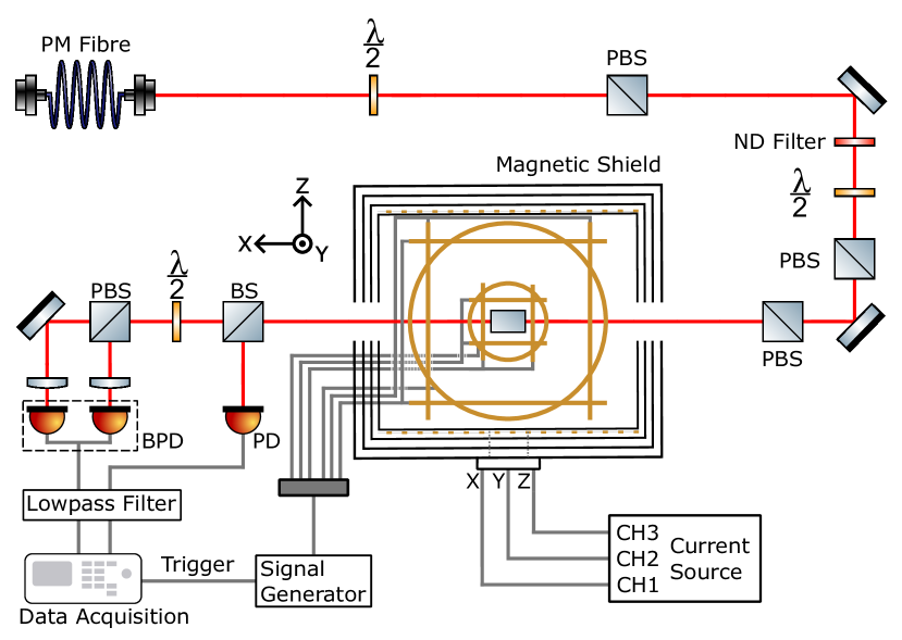
We implemented the zero-field magnetometry based on spin-alignment to a table-top, laboratory setup, see schematics in Fig. 1(c). Light with wavelength 895 nm resonant with the Cs D1 transition was emitted from a fiber pigtailed diode laser (Thorlabs DBR895PN). To adjust the intensity of light, a half-wave plate was employed in combination with a polarizer that aligned the polarization along the -axis. The light power (measured before the vapour cell) was 3 W for the data presented in Figs. 2, 3, 4, and 5, and 10 W for the data presented in Figs. 6 and 7. The linearly -polarized light entered a cubic vapor cell which was located in a four-layer mu-metal magnetic shield (Twinleaf MS-1L). The vapor cell is hand-blown, contains caesium atomic vapour, and is coated with paraffin. This leads to a long spin-coherence time. Following that, polarimetry is performed by employing a half-wave plate, a polarizing beam splitter and a balanced photodetector (Thorlabs PDB210A/M). The output from the balanced photodetector is subsequently directed through a 2 kHz low-pass filter and recorded with a data acquisition card within the computer for further analysis. For the absorption measurements (presented in Sec. IV.2), the transmitted light intensity was measured directly with a single photodetector (Thorlabs PDA36A2) placed immediately after the vapour cell outside the magnetic shield. The caesium cell is positioned within three sets of coils, where each coil set can be used to apply fields in three (, , ) directions. With no current applied to the coils, there is a small residual magnetic field inside the shield which is on the order of 100 nT. The outer coil set (which comes as standard with the Twinleaf MS-1L magnetic shield) is used to apply a static field to compensate the residual magnetic field in order for us to completely null the total magnetic field. The middle coil set is a three-axis cubic Helmholtz coil set which can be used to generate a linearly sweeping magnetic field which is used in the procedure for nulling the static field. The inner coil set, which is also a three-axis cubic Helmholtz coil, is used for generating different signals , e.g. a sinusoidal magnetic field for characterizing the magnetometer response and sensitivity or a synthetic cardiac signal. The total magnetic field can be written as
| (20) |
IV Results and Discussions
IV.1 Method for nulling the static field

We now experimentally demonstrate how to utilize the polarization rotation signal to null the total static magnetic field . This involves systematically sweeping magnetic fields applied in the and directions, and then changing the applied static field until a zero signal is obtained. In that case, the total static field should be as seen by Eqs. (18) and (19). The nulling procedure can be done iteratively, and the results presented here were all recorded in conditions close to zero total static magnetic field.
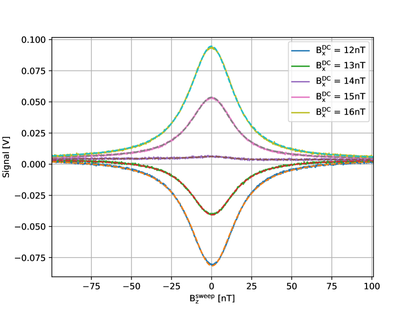
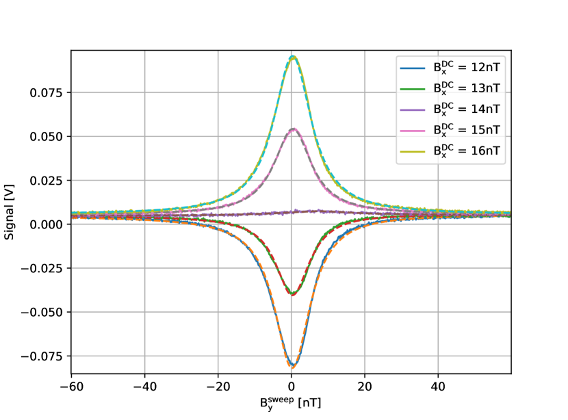
Figure 2(a) presents the measured signals with a linearly sweeping applied magnetic field in the direction. For these measurements, the static field component was varied within the range of 12 nT to 16 nT, while the other components were fixed at nT and nT. These settings correspond to a total static magnetic field close to zero. The observed signals looks like Lorentzian lineshapes as predicted by our model, see Eq. (19), when and . Note that for nT, the signal transforms into a flat line as predicted by Eq. (19) when and . For this setting, the applied static magnetic field precisely cancels the residual magnetic field leading to a net zero static magnetic field .
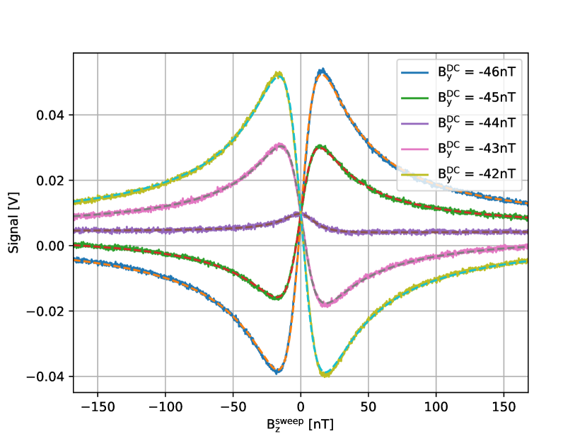
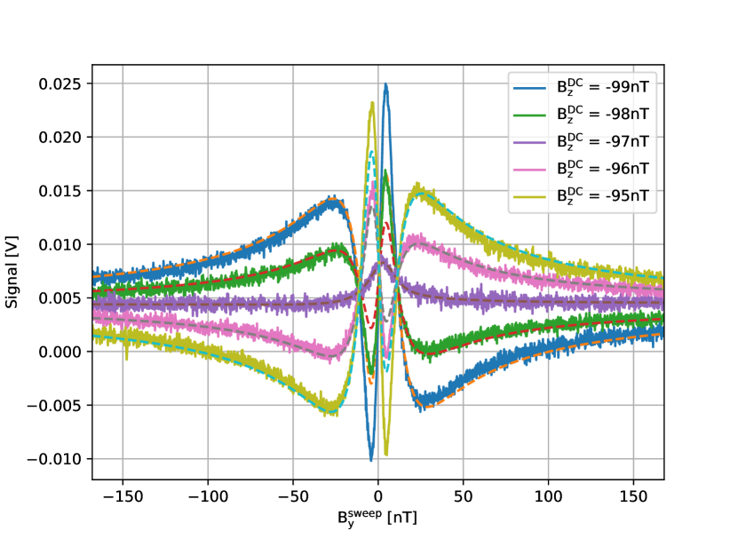
Measurements of the signal while sweeping the applied field in the direction are also obtained when varying the applied static field component. Those results are presented in Fig. 2(b). The lineshapes now look dispersive, as predicted by Eq. (19) with and .
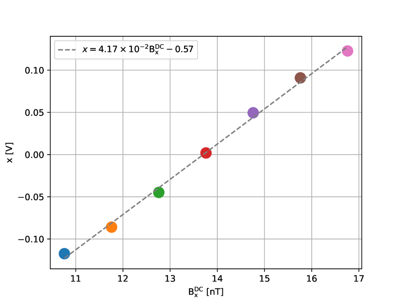
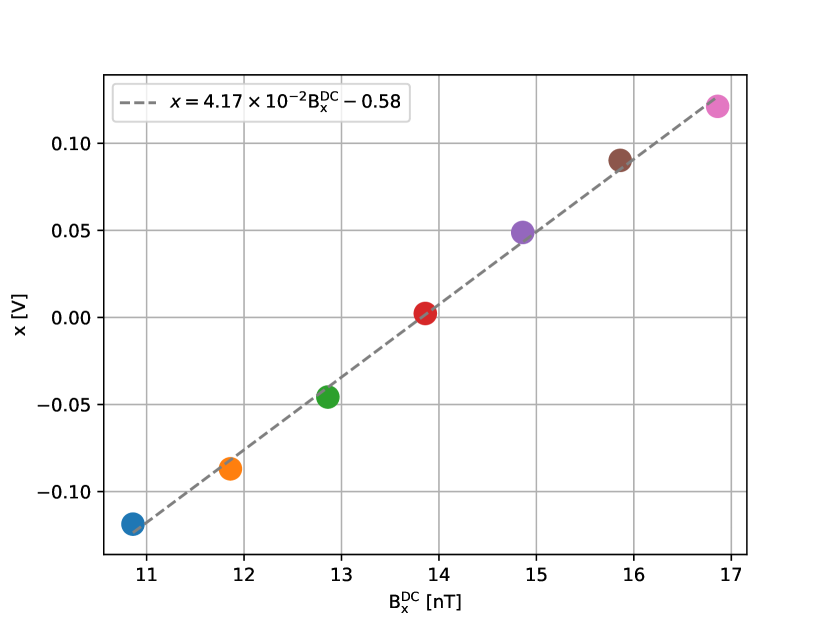
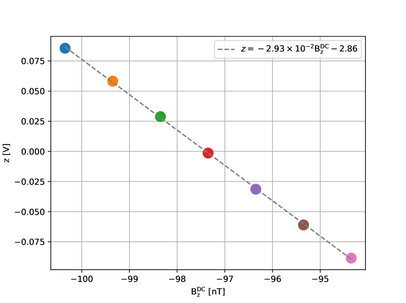
The obtained data in Figs. 2(a) and 2(b) are fitted to Eq. (19). Figure 2(c) shows the parameter obtained by fitting the data in Fig. 2(a). As expected, we see a linear relationship between the applied static field and the total static field. The parameter (not shown) was also fitted for the data in Fig. 2(a) and was found to be much smaller than . Figure 2(d) shows the parameter obtained for the data in Fig. 2(b). Again we see a linear relationship. The parameter (not shown) was also fitted for the data in Fig.2(b) and was found to be much smaller than .
The procedure is now repeated but with instead sweeping a field applied in the direction. Results are shown in Fig. 3. We see that it is possible to to adjust the and magnetic field components until the measured signal reaches zero. As mentioned, the nulling procedure can be repeated iteratively, until one obtains a signal very close to zero, for some specific settings of , , and . The total static field has then been nulled to better than a small fraction of a nT, as seen in Figs. 2(c), 2(d), 3(c) and 3(d) which is much smaller than the linewidth of the magnetic resonances, and therefore sufficient for zero-field magnetometry. A larger range where is varied from -40 nT to +40 nT can be seen in Appendix C in the Supplemental Material where the data is fitted to Eq. (11).
IV.2 Zero-field resonances measured by absorption
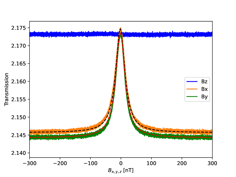
Having nulled the total static magnetic field, we now measure the zero-field resonances using absorption, i.e. by measuring the intensity of the transmitted light using a single detector placed immediately after the vapour cell. If a magnetic field is applied, it affects the quantum state of the caesium atoms as calculated in Eq. (II.1) and will lead to less light being transmitted through the vapour cell. To first order, the atoms are only sensitive to the magnetic field components and which are transverse to the light propagation direction. Figure 4 shows the sequential sweeping of the three components of the magnetic field using triangular ramps of ±300 (nT). We see that the signal is constant when sweeping , and that the signal has a Lorentzian lineshape when sweeping either or , as expected from Eqs. (13), (14) and (15). Due to the constant / Lorentzian lineshapes, a direct measurement of the intensity of the transmitted light is not useful for determining the magnetic field components, as several field values, e.g. & , or & give rise to the same transmitted light intensity, which means that one cannot uniquely infer a field component from the signal. However, we note that it is possible to measure all components of the magnetic field using modulation techniques, where several auxiliary oscillating magnetic fields are applied [28, 29].

IV.3 Zero-field magnetometry measured by polarization rotation
IV.3.1 Magnetic resonance
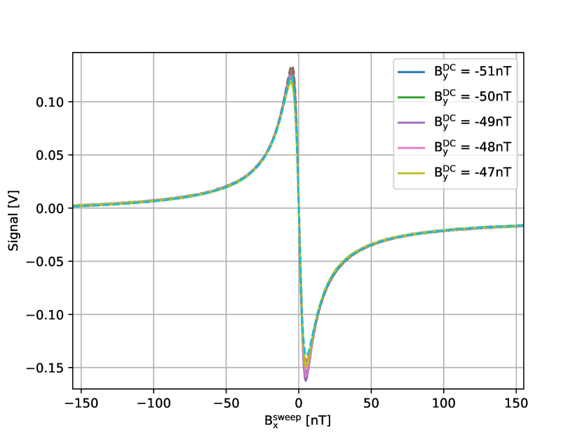
We now continue with demonstrating zero-field magnetometry by detecting the change in linear polarization of the transmitted light. As mentioned, this is done using polarimitry and a balanced photodetector. After having nulled the total static magnetic field, we apply a linearly sweeping magnetic field in the direction with strength ranging from -150 nT to 150 nT and measure the signal for various applied and static fields. These measurements are presented in Figs. 5(a) and 5(b). As seen, the signal exhibits a dispersive lineshape and is more or less unaffected by variations in the static magnetic field components as predicted by our theoretical model, see Eq. (16). I.e., in zero-field conditions, the magnetometer is only sensitive to changes in the component of the magnetic field.
IV.3.2 Bandwidth
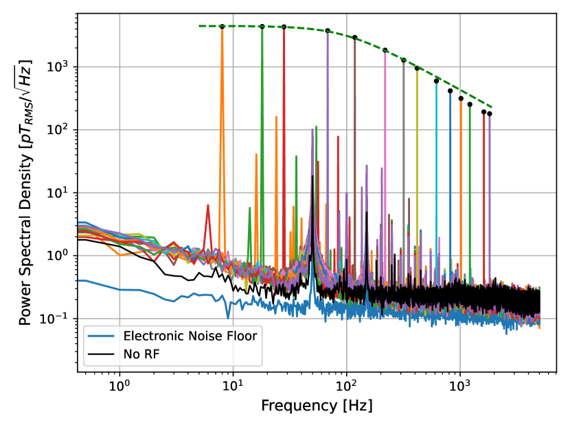
We now stop sweeping any magnetic fields. The bandwidth of the zero-field magnetometer is then assessed by sequentially applying 14 different sinusoidal magnetic fields with constant amplitude 3.16 and varying frequency ranging from 8 Hz to 1818 Hz. Two additional measurements were conducted in which the sinusoidal field was not applied (denoted “No RF”) and where the balanced photodetector was disconnected from the data-acquisition card (denoted “Electronic Noise Floor”). These two measurements were performed to assess the noise level of the magnetometer and of the electronic noise of the data acquisition card. For each of the measurements, the power spectral density of the signal was calculated and plotted in Fig. 6. Each of the 14 spectra have a sharp peak at the frequency corresponding to the respective oscillation. Those peak heights were fitted as a function of frequency to the response of a first order low-pass filter, i.e. the function . The low-pass filter response function has been derived for another type of zero-field OPM based on a spin-oriented atomic ensemble [10] but is here used phenomenologically to describe the response of our alignment based magnetometer. The fit allows us to extract the cut-off frequency Hz which is the magnetometer bandwidth. We would expect this number to equal the half width at half maximum of the magnetic resonances in Fig. 5 which is 11 nT corresponding to 39 Hz (when multiplying with the gyromagnetic ratio), however, we do experimentally find that the numbers differ by a factor of 2-3.
IV.3.3 Sensitivity
The noise floor of the magnetometer obtained with “No RF” depends on frequency as seen from Fig. 6. It is at 1 Hz and then improving to between 10 Hz and 100 Hz. Our experimentally obtained sensitivity is mainly limited by the electronic noise of our balanced photodetector (data not shown) together with a contribution from the electronic noise of the data acquisition card.
The sensitivity of an optically pumped magnetometer is fundamentally limited by quantum fluctuations in the atomic spin and the light shot noise such that the total quantum noise equals . The spin-projection noise can be written as [22]
| (21) |
where is the Bohr magneton, = 1/4 for the caesium ground state, is the number density of caesium atoms at room temperature (18.5∘C) [24] and is the volume of our vapor cell. is the transverse relaxation time and is calculated as ms, where we used the nT fitted in Fig. 5 and the gyromagnetic ratio for caesium which can be expressed as Hz/nT. Ideally, an optically pumped magnetometer has such that the total quantum noise . Hence the quantum noise limit for our magnetometer is .
IV.3.4 Synthetic magnetocardiography signal
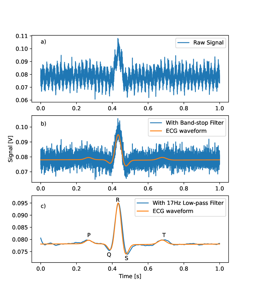
In order to determine if the performance of the magnetometer meets the standards for biomagnetic measurements, particularly magnetocardiography (MCG), a synthetic cardiac signal is applied in the direction with an amplitude of 100 pT peak-to-peak. This amplitude corresponds to the magnetic field of an adult person’s heart [33, 34] The waveform was generated using the stored electrocardiogram (ECG) waveform in a function generator (RIGOL DG1032Z) connected to one of the coils. Figure 7a shows the raw magnetometer signal, which is not averaged, and was recorded with a 10 kHz sampling rate. The signal is relatively noisy, but simple signal post-processing done by first a 49-51 Hz bandstop filter (to block 50 Hz noise), see Fig. 7b, and then a 17 Hz low-pass filter (to block high-frequency noise), see Fig. 7c, significantly improves the signal quality. We see that the filtered magnetometer signal looks very similar to the ECG waveform from the function generator. In particular, the real-time measurements captured by the magnetometer reveal the presence of the QRS complex and P and T waves which are features in the cardiogram which are important for medical doctors when assessing the health of a heart.
V CONCLUSIONS
In this study, we investigate the use of spin-aligned atomic ensembles for zero-field magnetometry. A novel method is introduced, which involves assessing the polarization rotation in transmitted light through an atomic vapor. We derive analytical expressions for the generated spin alignment and photodetection signals. By analyzing the obtained polarization rotation signal, we null the magnetic field components through an iterative procedure that adjusts the applied magnetic fields until a zero signal is achieved, indicating the absence of any static magnetic field. Achieving a zero-field environment is important for several applications, including nuclear magnetic resonance (NMR) gyroscopes [35, 36], and for biomedical measurements, such as magnetoencephalography (MEG) and magnetocardiography (MCG) where non-zero field components leads to artifacts or systematic errors [37]. Our method for nulling the field could potentially be employed in such applications, as demonstrated here by successfully detecting a synthetic cardiac signal. As opposed to other methods, e.g. using circular polarized light with several modulation fields, our method is modulation-free. After nulling the field, our magnetometer measures one component of the field using a single laser beam. If instead of using a paraffin-coated vapour cell (where all atoms inside the cell are probed), one uses a buffer-gas cell [24] (where only atoms inside the beam volume are probed), a vector magnetometer could in principle be implemented using three non-overlapping laser beams. Future work could investigate how to use only one or two laser linearly polarized beams for vector measurements.
We demonstrated a magnetic field sensitivity of at 1 Hz, which further improved to about 0.3 between 10 Hz and 100 Hz. The quantum limited sensitivity was calculated to meaning that further technical improvements are possible. Notably, some commercial optically pumped magnetometers have reached a sensitivity level of around fT/ [5], however they are operated at an elevated temperature C, as opposed to our magnetometer which was operated at room temperature. To enhance our sensitivity, various strategies can be explored, including the utilization of photodetectors with reduced electronic noise, multiple passes of the laser beam through the vapor cell, employing a larger vapor cell, increasing atom density through vapor cell heating, and using a repump laser beam to transfer atoms from the “dark” ground state back to the ground state, which is not probed by the laser light.
ACKNOWLEDGEMENTS
This work was supported by the QuantERA grant C’MON-QSENS! funded by the Engineering and Physical Sciences Research Council (EPSRC) (Grant No. EP/T027126/1), the Novo Nordisk Foundation (Grant No. NNF20OC0064182), and the University of Nottingham Hermes Award. Project C’MON-QSENS! is supported by the National Science Centre (2019/32/Z/ST2/00026), Poland under QuantERA, which has received funding from the European Union’s Horizon 2020 research and innovation programme under grant agreement no. 731473.
References
- Budker and Romalis [2007] D. Budker and M. Romalis, Nat. Phys. 3, 227 (2007).
- Wilson et al. [2019] N. Wilson, P. Light, A. Luiten, and C. Perrella, Phys. Rev. Applied 11, 044034 (2019).
- Kominis et al. [2003] I. Kominis, T. Kornack, J. Allred, and M. V. Romalis, Nature 422, 596 (2003).
- Fagaly [2006] R. L. Fagaly, Rev. Sci. Instrum. 77, 101101 (2006).
- Qus [2023] “Quspin,” https://quspin.com (2023).
- fie [2023] “Fieldline inc.” https://fieldlineinc.com/ (2023).
- twi [2023] “Twinleaf,” https://twinleaf.com/ (2023).
- Li et al. [2023] R. Li, Y. Liu, L. Cao, S. Li, J. Li, and Y. Zhai, Measurement 214, 112733 (2023).
- Le Gal and Palacios-Laloy [2022] G. Le Gal and A. Palacios-Laloy, Phys. Rev. A 105, 043114 (2022).
- Jensen et al. [2018] K. Jensen, M. A. Skarsfeldt, H. Stærkind, J. Arnbak, M. V. Balabas, S.-P. Olesen, B. H. Bentzen, and E. S. Polzik, Sci. Rep. 8, 16218 (2018).
- Marmugi and Renzoni [2016] L. Marmugi and F. Renzoni, Sci. Rep. 6, 23962 (2016).
- Brookes et al. [2022] M. J. Brookes, J. Leggett, M. Rea, R. M. Hill, N. Holmes, E. Boto, and R. Bowtell, Trends in Neurosciences (2022).
- Xia et al. [2006] H. Xia, A. Ben-Amar Baranga, D. Hoffman, and M. Romalis, Appl. Phys. Lett. 89, 211104 (2006).
- Sander et al. [2012] T. Sander, J. Preusser, R. Mhaskar, J. Kitching, L. Trahms, and S. Knappe, Biomed. Opt. Express 3, 981 (2012).
- Wyllie et al. [2012] R. Wyllie, M. Kauer, R. T. Wakai, and T. G. Walker, Opt. Lett. 37, 2247 (2012).
- Rushton et al. [2022] L. M. Rushton, T. Pyragius, A. Meraki, L. Elson, and K. Jensen, Rev. Sci. Instrum. 93, 125103 (2022).
- Bevington et al. [2019] P. Bevington, R. Gartman, and W. Chalupczak, J. Appl. Phys. 125 (2019).
- Romalis and Dang [2011] M. V. Romalis and H. B. Dang, Materials today 14, 258 (2011).
- Boto et al. [2018] E. Boto, N. Holmes, J. Leggett, G. Roberts, V. Shah, S. S. Meyer, L. D. Muñoz, K. J. Mullinger, T. M. Tierney, S. Bestmann, et al., Nature 555, 657 (2018).
- Borna et al. [2020] A. Borna, T. R. Carter, A. P. Colombo, Y.-Y. Jau, J. McKay, M. Weisend, S. Taulu, J. M. Stephen, and P. D. Schwindt, Plos one 15, e0227684 (2020).
- Weis et al. [2006] A. Weis, G. Bison, and A. S. Pazgalev, Phys. Rev. A 74, 033401 (2006).
- Ledbetter et al. [2007] M. P. Ledbetter, I. M. Savukov, V. M. Acosta, D. Budker, and M. Romalis, Phys. Rev. A 75, 032107 (2007).
- Di Domenico et al. [2007] G. Di Domenico, H. Saudan, G. Bison, P. Knowles, and A. Weis, Phys. Rev. A 76, 023407 (2007).
- Rushton et al. [2023] L. M. Rushton, L. Elson, A. Meraki, and K. Jensen, Phys. Rev. Applied 19, 064047 (2023).
- Savukov et al. [2005] I. M. Savukov, S. Seltzer, M. Romalis, and K. Sauer, Phys. Rev. Lett. 95, 063004 (2005).
- Zigdon et al. [2010] T. Zigdon, A. Wilson-Gordon, S. Guttikonda, E. Bahr, O. Neitzke, S. Rochester, and D. Budker, Opt. Express 18, 25494 (2010).
- Ingleby et al. [2018] S. J. Ingleby, C. O’Dwyer, P. F. Griffin, A. S. Arnold, and E. Riis, Phys. Rev. Applied 10, 034035 (2018).
- Beato et al. [2018] F. Beato, E. Belorizky, E. Labyt, M. Le Prado, and A. Palacios-Laloy, Phys. Rev. A 98, 053431 (2018).
- Bertrand et al. [2021] F. Bertrand, T. Jager, A. Boness, W. Fourcault, G. Le Gal, A. Palacios-Laloy, J. Paulet, and J. M. Léger, Rev. Sci. Instrum. 92, 105005 (2021).
- Wang et al. [2022] B. Wang, X. Peng, H. Wang, W. Xiao, and H. Guo, Sensors 22, 4184 (2022).
- Steck [2023] D. A. Steck, “Cs D Line Data,” https://steck.us/alkalidata/cesiumnumbers.1.6.pdf (2023).
- Auzinsh et al. [2014] M. Auzinsh, D. Budker, and S. M. Rochester, Optically polarized atoms: understanding light-atom interactions (Oxford University Press, 2014).
- Bison et al. [2009] G. Bison, N. Castagna, A. Hofer, P. Knowles, J.-L. Schenker, M. Kasprzak, H. Saudan, and A. Weis, Appl. Phys. Lett. 95, 173701 (2009).
- Sander et al. [2020] T. Sander, A. Jodko-Władzińska, S. Hartwig, R. Brühl, and T. Middelmann, Advanced Optical Technologies 9, 247 (2020).
- Walker and Larsen [2016] T. Walker and M. Larsen (Academic Press, 2016) pp. 373–401.
- Eklund [2008] E. J. Eklund, Microgyroscope based on spin-polarized nuclei, Ph.D. thesis, University of California, Irvine (2008).
- Borna et al. [2022] A. Borna, J. Iivanainen, T. R. Carter, J. McKay, S. Taulu, J. Stephen, and P. D. Schwindt, NeuroImage 247, 118818 (2022).