Enhanced bunching of nearly indistinguishable bosons

Abstract

In multiphoton interference processes, the commonly assumed direct link between boson bunching and particle indistinguishability has recently been challenged in Seron et al. [Nat. Photon. 17, 702 (2023)]. Exploiting the connection between optical interferometry and matrix permanents, it appeared that bunching effects may surprisingly be enhanced in some interferometers by preparing specific states of partially distinguishable photons. Interestingly, all the states giving rise to such an anomalous bunching were found to be far from the state of perfectly indistinguishable particles, raising the question of whether this intriguing phenomenon might even exist with nearly indistinguishable particles. Here, we answer positively this physically motivated question by relating it to a mathematical conjecture on matrix permanents whose physical interpretation had not yet been unveiled. Using a recently found counterexample to this conjecture, we demonstrate that there is an optical set-up involving 8 photons in 10 modes for which the probability that all photons bunch into two output modes can be enhanced by applying a suitable perturbation to the polarization states starting from photons with the same polarization. We also find out that the perturbation that decreases the bunching probability the most is not the one that takes the perfectly indistinguishable state towards a fully distinguishable state, as could naively be expected.

1 Introduction

In recent years, significant strides have been made in the advancement of photonic quantum technologies, driven by its wide-ranging applications in quantum communication, quantum computing, and quantum metrology [1]. Central to the success of these applications lies the capability to generate, manipulate, and detect multiple photons, which has seen a remarkable progress. In particular, this has led to one of the first experimental claims of quantum computational advantage over any classical algorithm [2] for solving the boson sampling problem [3].

Despite these remarkable developments, photonic quantum technologies are constrained by experimental limitations. In addition to the challenges posed by photon losses and various sources of noise, a noteworthy constraint arises from the fact that photons possess various internal degrees of freedom, such as polarization or time-frequency, and conventional photon sources do not yield ideal, perfectly indistinguishable photons. This difficulty prompts an exploration of linear interference with partially distinguishable photons, the intermediate realm between fully distinguishable photons – governed by classical stochastic processes – and fully indistinguishable photons, where quantum superposition and bosonic statistics come into play [4, 5].

The indistinguishability of bosons is at the origin of remarkable quantum interference phenomena, such as the celebrated Hong-Ou-Mandel (HOM) effect [6], which arises from the impossibility of distinguishing the situation in which two identical photons have crossed a 50:50 beam splitter from the trajectory in which they have both been reflected. Destructive interference leads to the bunching of the two photons in the same output mode, an effect that becomes less pronounced as soon as the photons become partially distinguishable (two orthogonally-polarized photons do not bunch any more as they are perfecly distinguishable). Larger scale experiments involving many bosons provide a testbed for the fundamental study of more general boson bunching phenomena [7, 8, 9, 10]. The latter have been suggested as an efficient way to test the correct functioning of experiments which are difficult to simulate classically [8, 9], relevant not only in photonics but also in atomic physics [10].

A natural way to quantify bunching is to measure the probability that all photons coalesce in the same output mode of an interferometer, which can be seen as a measure of indistinguishability [4, 7]. However, in experiments involving many photons, this quantity is difficult to assess as this probability is exponentially small in the photon number. This motivates the study of multimode bunching probabilities, i.e., the probability that all photons coalesce in some chosen subset of output modes. These are easier to measure and, in most practical cases, they decrease as the particles become more distinguishable [9, 11]. However, the behavior of multimode bunching probabilities with particle distinguishability is subtle. While numerical explorations and physical intuition strongly suggest that indistinguishable bosons should always maximize such bunching probabilities, it was recently demonstrated that this is not always the case. In Ref. [12], the authors have presented a family of optical set-ups, with 7 or more photons, in which partially distinguishable photons prepared in a specific polarization state can exhibit significantly higher multimode bunching probabilities than perfectly indistinguishable photons. These optical set-ups were found by building upon a mathematical conjecture on matrix permanents stated by Bapat and Sunder in 1985 [13] and recently disproved by Drury [14].

In Ref. [12], an open question remained about the behavior of multimode bunching probabilities for input states in the vicinity of the state of perfectly indistinguishable photons. In fact, all states found to lead to anomalous bunching in Ref. [12] happened to be located far from the perfectly indistinghuishable state. Moreover, any perturbation to this perfectly indistinguishable state was shown to leave multimode bunching probabilities invariant (to the first order), suggesting that it could be a local maximum.

In this paper, we investigate in depth the behavior of multimode bunching probabilities for nearly indistinguishable bosons, revealing several counterintuitive phenomena and, in particular, contradicting the above assumption about a local maximum. First, we connect the question of whether boson bunching can only decrease after a small perturbation to the state of indistinguishable bosons to a different conjecture on matrix permanents introduced by Bapat and Sunder in 1986 [15], whose physical meaning had not yet been understood. Furthermore, we convert a recent mathematical counterexample to this conjecture [16] into a linear optical circuit, implying that multimode bunching can be actually be enhanced by applying a suitable perturbation to the photons’ internal states. The found set-up requires 8 photons passing through a 10-mode interferometer and the perturbation requires only the ability to manipulate a two-dimensional internal degree of freedom such as polarization. As a side result, we prove a new implication between properties of permanents of positive semidefinite matrices, establishing a logical implication between two different conjectures from Bapat and Sunder. We believe this result may be of independent interest in the mathematics literature as the investigation of conjectures related to permanents of positive semidefinite matrices is an active research topic, in particular, due to its connection to the long-standing Lieb’s permanental dominance conjecture [17].

Finally, motivated by a better understanding of the sensitivity of bunching probabilities to perturbations, we investigate what kind of perturbations reduce bunching the most. Unexpectedly, we show that perturbations of a two-dimensional degree of freedom (such as polarization) can decrease bunching even more than a perturbation towards the state of fully distinguishable particles, which necessarily involves at least an $n$-dimensional degree of freedom for $n$ photons.

We hope our work motivates further studies about the role of particle distinguishability in the phenomenon of boson bunching as well as experiments testing its counterintuitive behavior.

2 Preliminaries

In this section, we will introduce some preliminary concepts central to this work, starting with linear interferometry, boson bunching, partial distiguishability, and then proceeding to mathematical conjectures concerning matrix permanents and their physical interpretation. Throughout the work we will have in mind photonic implementations, where it is easier to implement arbitrary interferometers. However, our results apply for any particle obeying bosonic statistics going through a linear interferometry process, which is also possible to implement in atomic experiments [10].

2.1 Multimode boson bunching

Consider an $m\times m$ unitary matrix $U$, which represents an $m$-mode linear interferometer. We send $n$ photons, into the first $n$ modes of this interferometer, with one photon per mode. TWe consider the photons to be in a pure, non-entangled state as illustrated in Fig. 1.

In addition to being described by the spatial mode of the interferometer, the state of the photon also depends on internal characteristics, such as spectral distribution or polarization. The wave function $\left|{\phi_{j}}\right\rangle$ describes the internal state of the photon upon entering mode $j$ of the interferometer. In this context, we assume that the interferometer keeps the internal state of the photon unchanged and only affects the spatial mode [4, 18, 5]. Specifically, the interferometer is represented by the operator $\hat{U}$, which performs the following action

$$\hat{U}\hat{a}^{\dagger}_{j,\phi_{j}}\hat{U}^{\dagger}=\sum_{k}U_{jk}\hat{a}^{\dagger}_{k,\phi_{j}},~{}~{}\forall j,$$ (1)

where $\hat{a}^{\dagger}_{j,\phi_{j}}$ is the creation operator which creates a photon in spatial mode $j$ in the internal state $\left|{\phi_{j}}\right\rangle$.

The object of study of our work are multimode bunching probabilities, also called generalized bunching probabilities [9, 10], which is the probability of finding all the photons in a subset $\mathcal{K}$ of the output modes. The multimode bunching probability, which we refer to as $P_{n}$, depends on the linear interferometer $U$ and the subset $\mathcal{K}$ via the positive semidefinite (p.s.d.) matrix $H$ defined as

$$H_{a,b}=\sum_{l\in\mathcal{K}}U_{l,a}^{*}U_{l,b}.$$ (2)

Naturally, $P_{n}$ also depends on the $n\times n$ Gram matrix referred to as the distinguishability matrix [4, 5], constructed from all possible overlaps of the internal wave functions of the input photons. The matrix is defined as

$$S_{i,j}=\left\langle{\phi_{i}}\middle|{\phi_{j}}\right\rangle.$$ (3)

For a fixed interferometer $U$ and subset $\mathcal{K}$, the dependency of the multimode bunching probability as a function of the distinguishability matrix $S$ is expressed via the following equation [9, 4]

$$P_{n}(S)=\text{perm}\left({H\odot S^{T}}\right).$$ (4)

Here, $H\odot S^{T}$ represents the Hadamard product (element-wise product) between the two matrices [9], with $(H\odot S^{T})_{ij}=H_{ij}S_{ji}$, while $\text{perm}\left({\cdot}\right)$ denotes the matrix permanent.

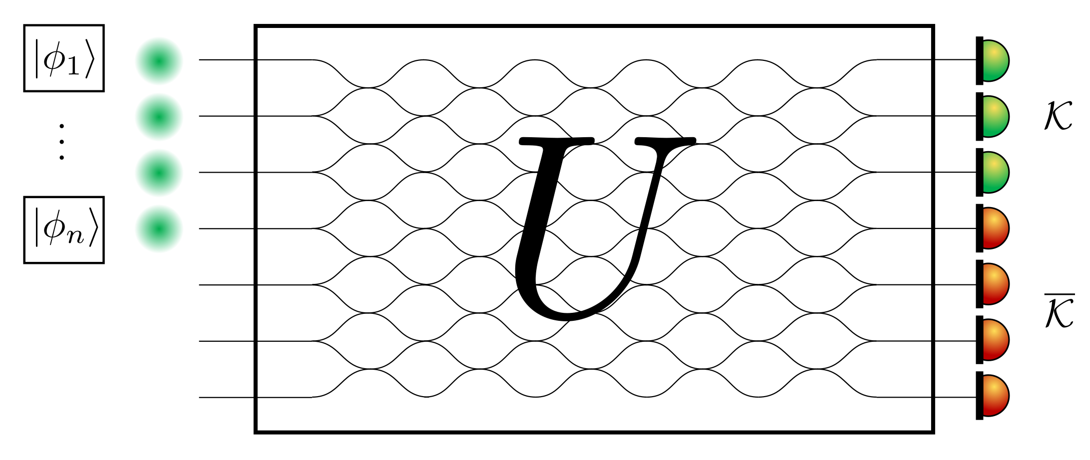
Figure 1: Interferometric setup. Photons are individually sent through the first $n$ input modes of a linear interferometer $U$ with $m$ modes, This interferometer can always be decomposed into a network of two-mode couplers [19]. Each photon at input $j$ carries specific internal degrees of freedom (e.g., polarization, arrival time) represented by an (internal) wave function $\left|{\phi_{j}}\right\rangle$. We are studying the probability that all $n$ photons bunch in a subset $\mathcal{K}$ (corresponding to the green detectors) for an input state of nearly indistinguishable photons, with internal wavefunctions $\left|{\phi_{j}}\right\rangle\approx\left|{\phi_{0}}\right\rangle$.

2.2 Conjectures related to boson bunching

2.2.1 Generalized Bunching

Interestingly, physical statements about boson bunching can be related to mathematical conjectures about matrix permanents that remained open for many years. Let us consider the following natural physical conjecture about multimode bunching

Conjecture P1 (Generalized Bunching).

Consider any linear interferometer and any nontrivial subset $\mathcal{K}$ of output modes. Among all possible input states of $n$ classically correlated photons, the probability that all photons are found in $\mathcal{K}$ is maximal if the photons are (perfectly) indistinguishable.

There was compelling evidence for the validity of this conjecture [9, 12], which generalizes the intuition obtained from the Hong-Ou-Mandel effect. In particular, the opposite statement about fermion antibunching is true: a state of indistinguishable fermions always minimizes multimode bunching probabilities [9]. Surprisingly, bosons do not always obey Conjecture P1, as was demonstrated in Ref. [12] via explicit counterexamples. Such counterexamples were built by exploiting the connection between this physical conjecture and a mathematical conjecture about permanents of p.s.d. matrices. Note that if we consider the particular case of input states discussed in Sec. 2.1, where each photon is in a pure state with internal wavefunction $\left|{\phi_{j}}\right\rangle$, we can summarize Conjecture P1 via the following mathematical statement

$$\text{perm}\left({H\odot S^{T}}\right)\stackrel{{\scriptstyle?}}{{\leq}}\text{perm}\left({H}\right).$$ (5)

Here, we used Eq. (4) as well as the fact that if all photons are indistinguishable, then $S=\mathbb{E}$ (with $\mathbb{E}_{i,j}=1$ for all $i,j$) and so $\text{perm}\left({H\odot\mathbb{E}}\right)=\text{perm}\left({H}\right)$. In this form, it is clear the relation with the following mathematical conjecture introduced in 1985 in an article by Bapat and Sunder [13].

Conjecture M1 (Bapat-Sunder 1985).

Let $\mathbf{H_{n}}$ be the set of $n\times n$ positive semi-definite Hermitian matrices. If $A$, $B$ $\in\mathbf{H_{n}}$, then

$$\text{perm}\left({A\odot B}\right)\leq\text{perm}\left({A}\right)\prod_{i=1}^{n}B_{ii}.$$ (6)

It was shown by Zhang [20] that, without loss of generality, we can restrict ourselves to the case where $B$ is a Gram matrix in which case $B_{ii}=1$. Thus, Conjecture M1 is equivalent to Eq. (5) and thus to Conjecture P1 restricted to pure, separable, input photon states. In Ref. [12] the authors used a counter-example to Conjecture M1 found by Drury [14] to find a family of interferometers and a polarisation state that contradicts the generalized bunching conjecture.

It is worth noting that another form of the generalized bunching conjecture has been formulated which considers an arbitrary state of input particles, possibly entangled, bunching in a subset of size $|\mathcal{K}|\geq n$ [9]. An even more general form of the conjecture, with entangled input states and arbitrary subset size, had been related to a different conjecture about permanents of p.s.d. matrices (the permanent-on-top conjecture) and a counterexample was found involving 5 photons bunching into 2 modes [21]. This and other mathematical arguments were part of the motivation to consider the restriction $|\mathcal{K}|\geq n$ in [9]. Even though it was not explicitly mentioned in Ref. [12], it is possible to see that this version of the generalized bunching conjecture is also false. We clarify in Appendix A that any counterexample to Conjecture P1 with $|\mathcal{K}|<n$ can be converted via a simple modification to a physical situation where multimode bunching probabilities on subsets of size $|\mathcal{K}|\geq n$ can also be enhanced by suitable states of partial distinguishabile bosons.

The focus of our work is in another question which was left open in Ref. [12] about whether the state of indistinguishable bosons is a local maximum for any multimode bunching probability.

2.2.2 A local version of generalized bunching

It was noticed in Ref. [12] that the distinguishability matrices realizing the counterexamples to the generalized bunching conjecture P1 are, in some sense, far from the Gram matrix corresponding to indistinguishable wavefunctions given by the all 1’s matrix $\mathbb{E}$. This can be seen, for example, by using the measure of indistinguishability [22, 4, 9]

$$d(S)=\frac{\text{perm}\left({S}\right)}{n!},$$ (7)

which measures the permutationally symmetric component of the wavefunction $\left|{\Phi}\right\rangle=\left|{\phi_{1}}\right\rangle\left|{\phi_{2}}\right\rangle...\left|{\phi_{n}}\right\rangle$. This measure takes the value $d(\mathbb{E})=1$ for indistinguishable bosons, whereas for the internal photon states of the counterexamples from Ref. [12] takes a value significantly smaller than $1$.This leads to a natural question: can multimode bunching probabilities be enhanced by partially distinguishable input states in the neighborhood of a state of indistinguishable bosons? The same question can be rephrased in the following way. If we fix the interferometer $U$ and the subset $\mathcal{K}$, we know that the multimode bunching probability $P_{n}(S)$, seen as a function whose argument is a Gram matrix, does not always have its global maximum for $S\equiv\mathbb{E}$. However, is this always a local maximum? The corresponding physical conjecture, which we see as a local version of the generalized bunching conjecture, can be stated as follows.

Conjecture P2 (Generalized bunching (local)).

Consider a state of $n$ indistinguishable bosons going through a linear interferometer described by a unitary $U$. For any such $U$ and any nontrivial subset $\mathcal{K}$ of output modes, the probability that all photons are bunching in $\mathcal{K}$ can only decrease if an infinitesimal perturbation is applied to the internal wavefunctions of the bosons, making them partially distinguishable.

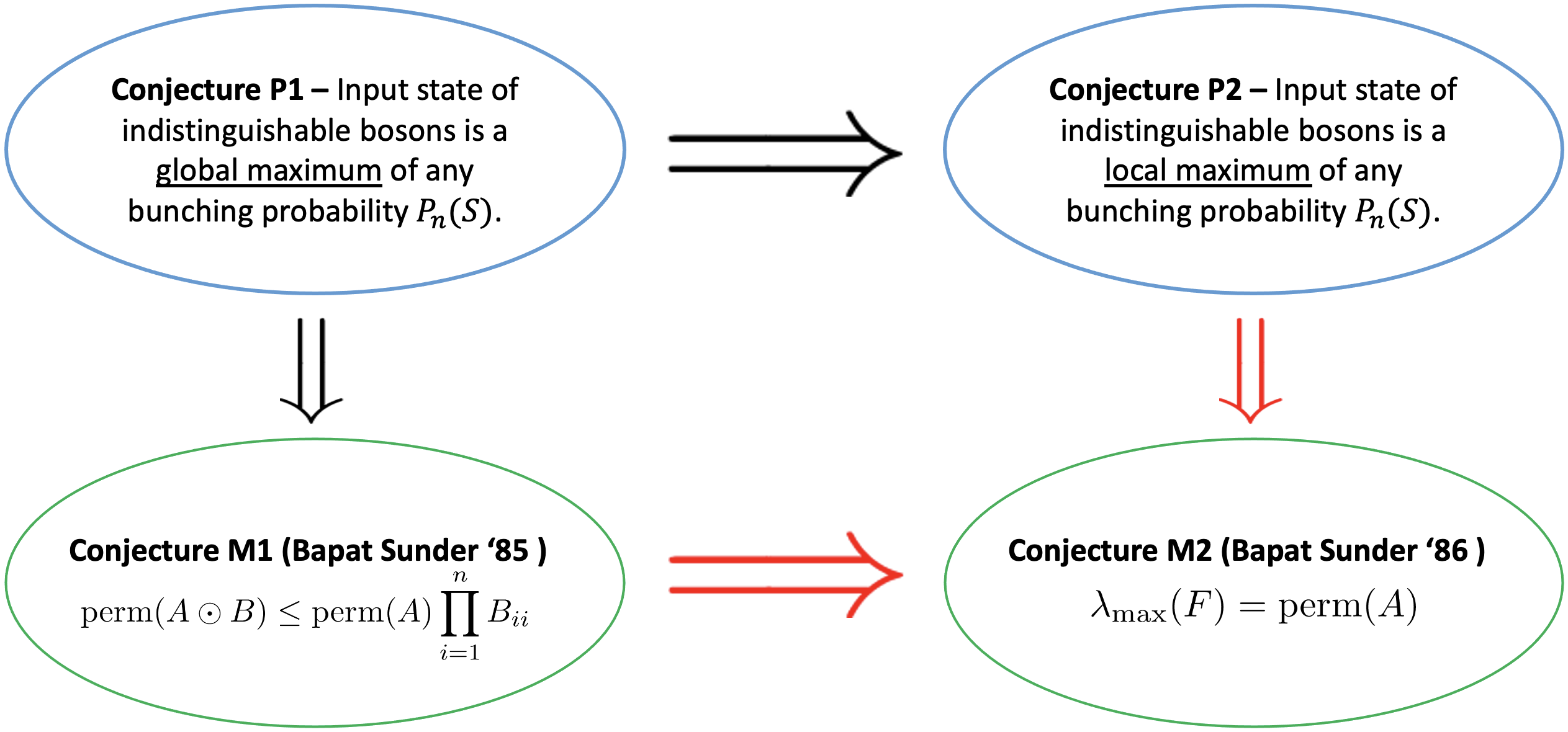
Figure 2: This figure summarises the implications between all the physical (labeled by P) and mathematical (labeled by M) conjectures presented in the section 2.2. It had already been noted that the validity of Conjecture P1 would require that Conjecture M1 is also valid [9, 12]. Our main contributions are represented by the red arrows: we introduce conjecture P2, a conjecture which is weaker than P1, and show that the validity of either conjecture P2 or M1 would imply that M2 is also true. In other words, any counterexample to conjecture M2 can be used to construct a counterexample to either P2 or M1.

Clearly, if Conjecture P1 were true than also Conjecture P2 would be true. Interestingly, by investigating this physically motivated question, we found a connection with a different mathematical conjecture which coincidently was also introduced by Bapat and Sunder, albeit in a different work [15], and also recently disproved by Drury [16]. The conjecture is stated as follows.

Conjecture M2 (Bapat-Sunder 1986).

Let $A$ be a positive definite matrix. Denote by $A(i,j)$ the $(n-1)\times(n-1)$ submatrix of $A$ obtained by deleting the $i$-th row and $j$-th column of $A$. Then $\text{perm}\left({A}\right)$ is the largest eigenvalue of the matrix $F$ such that $F_{i,j}=A_{i,j}\text{perm}\left({A(i,j)}\right)$.

The following sections are aimed at clarifying the connection between the physical Conjecture P2 about the behavior of generalized bunching probabilities under small distinguishability perturbations and the mathematical Conjecture M2. In particular, we show in Sec. 4 how to construct a counterexample to Conjecture P2 from a counterexample of Conjecture M2. Interestingly, this also implies a previously unknown implication relation between Conjecture M1 and M2, which may be of independent interest in mathematics. We demonstrate this implication in Appendix C without using any quantum mechanics jargon, so that it is accessible to a broader community. The relation between the different physical and mathematical conjectures, as well as our main new results, are summarized in Fig. 2.

3 Small perturbations to indistinguishable bosons

The core of our work is about analysing how multimode bunching probabilities behave when small perturbations are applied to otherwise indistinguishable photon wavefunctions. To define the most general perturbation applicable to indistinguishable photons, let us consider that each of the $n$ photons going through a different spatial mode of the interferometer have initially the same internal state $\left|{\phi_{0}}\right\rangle$. We apply a different small perturbation to each of the photons, such that perturbation of the $i$-th photon is proportional to an arbitrary normalized quantum state $\left|{\eta_{i}}\right\rangle$. After the perturbation, the $i$-th photon is in the state $|\tilde{\phi_{i}}\rangle$ which can be expressed as

$$|\tilde{\phi_{i}}\rangle=\frac{1}{\alpha_{i}}(\left|{\phi_{0}}\right\rangle+\epsilon v_{i}\left|{\eta_{i}}\right\rangle),$$ (8)

for $i$ going from $1$ to $n$, where $\epsilon$ is positive and the $v_{i}$’s are the components of an arbitrary complex vector $\bm{v}$ of constant norm. Without loss of generality we can choose $||\bm{v}||=1$, since this would boil down a rescaling of the components of $\bm{v}$ which can be absorbed by a redefinition of $\epsilon$, i.e. if $\bm{v}\rightarrow\bm{v}/||\bm{v}||$ and $\epsilon\rightarrow||\bm{v}||\epsilon$, the previous equation remains invariant. In addition, we define

$$\alpha_{i}=\frac{1}{\sqrt{1+2\epsilon.\mathfrak{Re}(v_{i}\left\langle{\eta_{i}}\middle|{\phi_{0}}\right\rangle)+\epsilon^{2}|v_{i}|^{2}}}$$ (9)

so that the perturbed state $|\tilde{\phi_{i}}\rangle$ remains normalized.

We start by proving a stability theorem showing that first order perturbations to the internal states do not change bunching probabilities (see Sec. 3.1). This statement and a sketch of the proof had already been given in Ref. [12] and here we present a more detailed proof. The connection to Conjecture M2 appears from a second order treatment, which we develop in Sec. 3.2.

3.1 Stability around the bosonic case

Considering a generic perturbation of the form Eq. (8), the distinguishability matrix of the perturbed states is given by

$$\tilde{S}_{i,j}=\left\langle{\tilde{\phi}_{i}}\middle|{\tilde{\phi_{j}}}\right\rangle=$$

$$\frac{1+\epsilon(v_{i}^{*}\left\langle{\eta_{i}}\middle|{\phi_{0}}\right\rangle+v_{j}\left\langle{\phi_{0}}\middle|{\eta_{j}}\right\rangle)+\epsilon^{2}v_{i}^{*}v_{j}\left\langle{\eta_{i}}\middle|{\eta_{j}}\right\rangle}{\alpha_{i}\alpha_{j}}.$$ (10)

We show the following stability theorem about bunching probabilities.

Stability Theorem.

Consider the multimode bunching probability into a subset $\mathcal{K}$ after a linear interference process described by the unitary matrix $U$. For an arbitrary choice of the perturbation parameters in Eq. (8) the multimode bunching probability is stable to first order, i.e.

$$\frac{\partial P_{n}(\tilde{S})}{\partial\epsilon}=0.$$ (11)

Proof.

Recalling the definition of the normalization factors $\alpha_{i}$ from Eq. (9), we can expand the perturbed distinguishability matrix $\tilde{S}$ from Eq. (3.1) to first order as

$$\tilde{S}_{i,j}=1+\epsilon\mathfrak{Im}(v_{i}^{*}\left\langle{\eta_{i}}\middle|{\phi_{0}}\right\rangle+v_{j}\left\langle{\phi_{0}}\middle|{\eta_{j}}\right\rangle)i+O(\epsilon^{2}),$$ (12)

where $\mathfrak{Im}$ stands for the imaginary part. To simplify the notations, it is useful to define the vector $\bm{x}$ and the matrix $\delta S$ such that

$$x_{i}=\mathfrak{Im}(v_{i}^{*}\left\langle{\eta_{i}}\middle|{\phi_{0}}\right\rangle),$$

$$\delta S_{i,j}=\epsilon~{}i(x_{i}-x_{j}).$$

This notation allows us to express the distinguishability matrix as follows

$$\tilde{S}=\mathbb{E}+\delta S+O(\epsilon^{2}).$$ (13)

According to Eq. (4), for a fixed interferometer $U$ and subset $\mathcal{K}$, the multimode bunching probability of the perturbed state can be expressed as,

$$\text{perm}\left({H\odot\tilde{S}^{T}}\right)=$$

$$\text{perm}\left({H\odot\mathbb{E}+H\odot\delta S^{T}+O(\epsilon^{2})}\right).$$ (14)

To compute the permanent of the sum of two matrices we use the formula presented in Eq. (B) of Appendix B. By applying this formula to Eq. (3.1), we derive

$$\text{perm}\left({H\odot\tilde{S}^{T}}\right)=\text{perm}\left({H}\right)$$

$$+\epsilon\sum_{i,j}^{n}(H\odot\delta S^{T})_{i,j}\text{perm}\left({H(i,j)}\right)+O(\epsilon^{2}).$$ (15)

For notational brevity, let us define

$$F_{i,j}=H_{i,j}\text{perm}\left({H(i,j)}\right),$$ (16)

which allows us to write the term proportional to $\epsilon$ in Eq. (3.1) in a simpler form

$$\sum_{i,j}^{n}(H\odot\delta S^{T})_{i,j}\text{perm}\left({H(i,j)}\right)=\sum_{i,j}^{n}i(x_{j}-x_{i})F_{i,j}.$$ (17)

Thus, the $F$ matrix appearing in Conjecture M2 appears naturally in a perturbative expansion of the bunching probabilities. This matrix has the following property: from the Laplace expansion of the permanent, we have for any choice of row or column of $F$ that

$$\sum_{i=1}^{n}F_{i,j}=\sum_{j=1}^{n}F_{i,j}=\text{perm}\left({H}\right).$$ (18)

Hence,

$$\sum_{i,j}^{n}i.(x_{j}-x_{i})F_{i,j}=$$

$$i\sum_{j}^{n}x_{j}\text{perm}\left({H}\right)-i\sum_{i}^{n}x_{i}\text{perm}\left({H}\right)=0,$$ (19)

which concludes the proof. ∎

The stability of bunching probabilities around the ideal bosonic case, further supports the idea that this case might be a local maximum (Conjecture P2). In what follows we show how to disprove this via a second-order expansion of the bunching probability.

3.2 Second-order analysis

In order to perform a second order expansion we will assume that the perturbation is performed in an orthogonal direction with respect to the initial internal wavefunction $\left|{\phi_{0}}\right\rangle$ in Eq. (8), i.e. $\left\langle{\eta_{i}}\middle|{\phi_{0}}\right\rangle=0,\forall i\in\{1,...,n\}$. This simplifies the analysis and it is sufficient to connect the variation of the multimode bunching probability to the statement of Conjecture M2. Using this assumption, the normalization factor is simplified to $\alpha_{i}=\frac{1}{\sqrt{1+\epsilon^{2}|v_{i}|^{2}}}$ and the perturbed Gram matrix can be written as

$$\tilde{S}_{i,j}=\left\langle{\tilde{\phi_{i}}}\middle|{\tilde{\phi_{j}}}\right\rangle=\frac{1+\epsilon^{2}v_{i}^{*}v_{j}\Delta_{i,j}}{\sqrt{(1+\epsilon^{2}|v_{i}|^{2})(1+\epsilon^{2}|v_{j}|^{2})}},$$ (20)

where we defined the Gram matrix associated to the perturbation $\Delta_{i,j}=\left\langle{\eta_{i}}\middle|{\eta_{j}}\right\rangle$. By applying Taylor’s expansion and neglecting the terms of $\mathcal{O}(\epsilon^{4})$, the Gram matrix becomes

$$\tilde{S}_{i,j}=1+\epsilon^{2}\Bigl{(}v_{i}^{*}v_{j}\Delta_{i,j}-\frac{|v_{i}|^{2}}{2}-\frac{|v_{j}|^{2}}{2}\Bigl{)}+\mathcal{O}(\epsilon^{4}).$$ (21)

As $\left|{\phi_{0}}\right\rangle$ and $\left|{\eta_{i}}\right\rangle$ are orthogonal for every $i$, there are no linear terms in $\epsilon$ in $\tilde{S}_{i,j}$. By defining the matrix $X$ such that $\tilde{S}_{i,j}=1+\epsilon^{2}X_{i,j}$, the probability of bunching for a fixed $H$ matrix is equal to

$$P_{n}(\tilde{S}) =\text{perm}\left({H\odot\tilde{S}^{T}}\right)$$ (22)

$$=\text{perm}\left({H+\epsilon^{2}H\odot X^{T}+O(\epsilon^{4})}\right).$$ (23)

Using once again Eq. (B) from Appendix B, we obtain

$$\text{perm}\left({H\odot\tilde{S}^{T}}\right)=\text{perm}\left({H}\right)+$$

$$\epsilon^{2}\sum_{i,j}^{n}(H\odot X^{T})_{i,j}\text{perm}\left({H(i,j)}\right)+O(\epsilon^{4}).$$ (24)

We note that this equation has no linear terms in $\epsilon$, which is consistent with the stability theorem. By replacing $X_{i,j}$ by its value, we obtain that the variation in the bunching probability, which we denote as $\delta P_{n}$, is given by

$$\ \delta P_{n}=\text{perm}\left({H\odot\tilde{S}^{T}}\right)-\text{perm}\left({H}\right)$$

$$\ =\epsilon^{2}\sum_{i,j}^{n}(v_{j}^{*}v_{i}\Delta_{j,i}-\frac{|v_{i}|^{2}}{2}-\frac{|v_{j}|^{2}}{2})F_{i,j}+O(\epsilon^{4}).$$ (25)

Our aim is to understand whether $\delta P_{n}$ can be strictly positive, which would show that bunching probabilities are not always locally maximized by a state of indistinguishable bosons. To do so we first demonstrate an upper bound on $\delta P_{n}$ related to the maximum eigenvalue of the $F$ matrix and subsequently we demonstrate how to saturate this upper bound. Since $\Delta$ is a Gram matrix, it admits a unique Cholesky decomposition

$$\Delta_{j,i}=\sum_{k=1}^{K}(u_{j}^{k})^{*}u_{i}^{k},$$ (26)

where $K$ is the rank of $\Delta$ and $\bm{u}^{k}$ is a set of $K$ $n$-dimensional vectors [23]. Using this fact together with Eq. (18) and $||\bm{v}||=1$, we can rewrite Eq. (3.2) as

$$\delta P_{n}= \epsilon^{2}\Bigl{(}\sum_{k=1}^{K}(\bm{v}\odot\bm{u^{k}})^{\dagger}F(\bm{v}\odot\bm{u^{k}})-\text{perm}\left({H}\right)\Bigl{)}$$

$$+O(\epsilon^{4}).$$ (27)

It is important to note that the matrix $F$ is also p.s.d., as shown in Appendix E, so the first term of the previous equation is always non-negative. Moreover, we can bound it by

$$\sum_{k=1}^{K}(\bm{v}\odot\bm{u}^{k})^{\dagger}F(\bm{v}\odot\bm{u}^{k})\leq||F||\sum_{k=1}^{K}||(\bm{v}\odot\bm{u}^{k})||^{2},$$ (28)

This can be further simplified by noting that

$$\sum_{k=1}^{K}||(\bm{v}\odot\bm{u}^{k})||^{2} =\sum_{k=1}^{K}\sum_{i}^{n}|v_{i}|^{2}|u^{k}_{i}|^{2}$$ (29)

$$=\sum_{i=1}^{n}|v_{i}|^{2}\Delta_{ii}=1.$$ (30)

Since the matrix norm $||F||=\lambda_{\max}(F)$ is given by the largest eigenvalue of $F$, we finally obtain the bound

$$\delta P_{n}\leq\epsilon^{2}(\lambda_{max}(F)-\text{perm}\left({H}\right))+O(\epsilon^{4}).$$ (31)

It is possible to see that this upper bound is saturated by choosing all the states $\left|{\eta_{i}}\right\rangle\equiv\left|{\phi_{1}}\right\rangle$, with $\left\langle{\phi_{0}}\middle|{\phi_{1}}\right\rangle=0$, which is equivalent to choosing the Gram matrix $\Delta=\mathbb{E}$. This matrix is of rank 1, and thus its Cholesky decomposition has a single vector $\bm{u}^{1}=(1,1,...,1)$. Plugging this in Eq. (3.2) we obtain

$$\delta P_{n}=\epsilon^{2}\Bigl{(}\bm{v}^{\dagger}F\bm{v}-\text{perm}\left({H}\right)\Bigl{)}+O(\epsilon^{4}),$$ (32)

and thus the upper bound from Eq. (31) is saturated if $\bm{v}\equiv\bm{v}_{\max}$ which is the eigenvector of the $F$ matrix with the largest eigenvalue. Clearly, $\delta P_{n}$ becomes positive if

$$\lambda_{max}(F)>\text{perm}\left({H}\right),$$ (33)

i.e. if the matrix $H$ is a counterexample to Conjecture M2. We will exploit this to build an explicit physical counterexample violating the local version of the generalized bunching conjecture (Conjecture P2), in which bunching probabilities can be enhanced if a small perturbations is applied to the wavefunctions of indistinguishable photons.

4 Enhancing bunching with nearly indistinguishable bosons

In 2018, Drury found an $8\times 8$ p.s.d. matrix $A$ that demonstrates that Conjecture M2 is false [14]. The matrix is defined as $A=M^{\dagger}M$, with

$$M =M_{R}+iM_{I},$$ (34)

$$M_{R} =\begin{pmatrix}-7&9&-6&3&7&4&0&5\\ 4&1&-8&-7&1&1&8&1\\ \end{pmatrix},$$

$$M_{I} =\begin{pmatrix}4&-3&2&4&6&-4&1&-8\\ -5&4&-2&4&-4&-8&-6&-3\\ \end{pmatrix}.$$

By calculating the matrix $F$ as defined in Conjecture M2, it can be seen that $\lambda_{max}(F)/\text{perm}\left({A}\right)\approx 1.017$, i.e. this example violates the conjecture by about $1.7\%$.

We will use this mathematical counterexample to construct a physical situation where bunching can be enhanced by perturbing a state of indistinguishable photons. It had already been noticed in Ref. [12] that given any p.s.d. matrix $A$, we can find an interferometer and a subset $\mathcal{K}$ such that the corresponding $H$ matrix in Eq. (2) is a rescaled version of $A$. In a nutshell, the idea is to embed $\sqrt{\alpha}M$ in the top left corner of $U$. The value of $\alpha$ is chosen such that $||\alpha M^{\dagger}M||=1$. To embed $\sqrt{\alpha}M$ into $U$ it is enough to choose $U$ to be a $10\times 10$ matrix. First we add two columns to the matrix $\sqrt{\alpha}M$ choosing these columns such that the newly constructed $2\times 10$ matrix has orthonormal rows which are normalized (see also Lemma 29 from Ref. [3]). Moreover, the lower part of $U$ (a $8\times 10$ matrix) can be constructed by generating 8 orthonormal row vectors, which are also orthogonal to the first two rows. Such $U$ could be implemented with a circuit of 36 beam splitters, using the decomposition from Clements et al [19]. All the data for the physical implementation are available on github, see Section ”Code availability”.

The physical experiment leading to a counterexample of Conjecture P2 involves thus an input state of 8 photons, as the number of photons is given by the size of the $H$ matrix, such that each photon goes through each one of the first 8 modes of a 10-mode interferometer. We look at the bunching probability in 2 output modes, since the rank of $H$ is 2, which can be chosen to be the first two output modes given the way we constructed $U$. We will see that this bunching probability can gradually increase by applying a suitable perturbation to the internal photon states. As demonstrated in Sec. 3.2, the upper bound on the variation of the bunching probability $\delta P_{n}$ from Eq. (31) is attained by perturbing the internal wavefunction of indistinguishable photons in a two-dimensional space spanned by two orthogonal states $\{\left|{\phi_{0}}\right\rangle,\left|{\phi_{1}}\right\rangle\}$. Naturally, we refer to these states as $\left|{\phi_{0}}\right\rangle\equiv\left|{H}\right\rangle$ and $\left|{\phi_{1}}\right\rangle\equiv\left|{V}\right\rangle$ since polarization gives a natural two-dimensional degree of freedom of the photon that can be manipulated, for instance, using waveplates. However, any two-dimensional subspace of the photon internal states could be used such as a time-bin encoding. We define the perturbed internal states as

$$|\tilde{\phi_{i}}\rangle=\frac{1}{\alpha_{i}}(\left|{H}\right\rangle+\epsilon~{}{(v_{\max})}_{i}\left|{V}\right\rangle),~{}$$ (35)

with $i\in\{1,..,8\}$, where $\alpha_{i}$ are normalization constants. Here, ${(v_{\max})}_{i}$ is the $i$th component of the normalized eigenvector corresponding to the largest eigenvector of the $F$ matrix constructed from Drury’s counterexample. By defining $F^{\prime}_{ij}=H_{ij}\text{perm}\left({H(i,j)}\right)$, which is a rescaled version of $F$, we obtain from Eq. (32) that the ratio between the bunching probability for the partially distinguishable perturbed states and its counterpart for indistinguishable bosons for small $\epsilon$ is given by

$$R(\epsilon) =\frac{\text{perm}\left({H\odot\tilde{S}^{T}}\right)}{\text{perm}\left({H}\right)},$$ (36)

$$\approx 1+\epsilon^{2}\left(\frac{\lambda_{\max}(F^{\prime})}{\text{perm}\left({H}\right)}-1\right),$$ (37)

$$\approx 1+0.017\epsilon^{2},$$ (38)

where we have neglected terms of $O(\epsilon^{4})$.

Although our perturbative analysis is only accurate for a small enough perturbation strength $\epsilon$, we can exploit numerically larger ranges of this parameter. In Fig. 3 we show that the violation ratio $R(\epsilon)$ peaks at a value of $\epsilon_{\max}\approx 1.2$ leading to a bunching enhancement of about $2\%$. Although a small effect, it is enough to show that the state of indistinguishable photons do not locally maximize bunching probabilities in the space of possible input states. We leave as an open question whether bigger bunching enhancements can be observed. This would be important to make the experimental observation of this phenomenon more feasible. In fact, the absolute value of the multimode bunching probability at $\epsilon_{\max}$ is equal to $P_{n}(S(\epsilon_{max}))\approx 1.353\times 10^{-3}$, in comparison for indistinguishable particles $P_{n}(S(0))\approx 1.327\times 10^{-3}$, making it challenging to measure this effect with current technology.

It is also interesting to examine the evolution of photon indistinguishability as a function of $\epsilon$, according to the measure from Eq. (39)

$$d(\tilde{S}(\epsilon))=\frac{\text{perm}\left({\tilde{S}(\epsilon)}\right)}{n!},$$ (39)

for the chosen parametrization of the input states. We plot this quantity in Fig. 4 showing it always decreases monotonically for the range of $\epsilon$ we explored. This adds to the previous result from Ref. [12], showing once again that even though this measure is directly proportional to single-mode bunching probabilities [4], there is no straightforward link between multimode bunching probabilities and this measure of indistinguishability. The maximum value of $d(S(\epsilon))$ is approximately equal to $0.281$. As a comparison, for the 7-photon counterexample of the generalized bunching conjecture from Ref. [12], the indistinguishability measure $d(S)\approx 8.93\times 10^{-3}$, which is significantly lower than the values presented in Fig. 4. We also remark that the $H$ matrices from the counterexamples of Ref. [12] are not counterexamples to conjecture M2, showing they cannot be used to find violations of the local version of the generalized bunching conjecture using our construction.

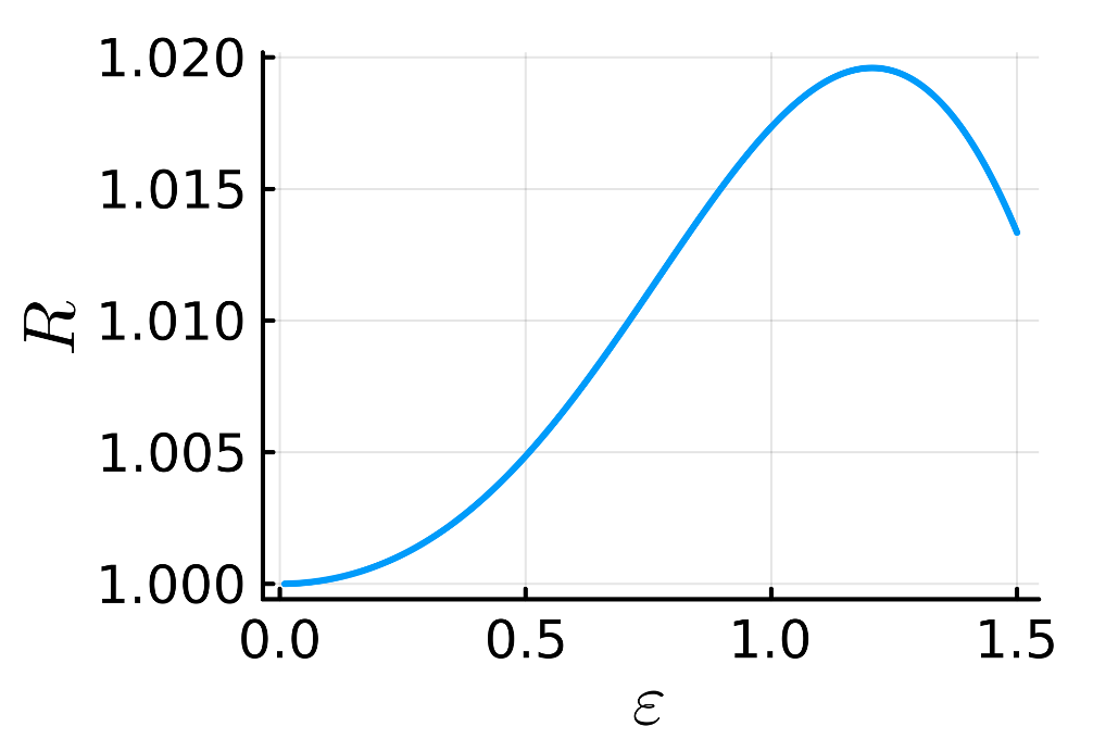
Figure 3: The Violation ratio $R(\epsilon)$ (Eq. (36)) quantifying the relative enhacement of the bunching probability as a function of the perturbation strength $\epsilon$. In the region of $\epsilon$ explored in the plot, the ratio $R(\epsilon)$ is always larger than $1$ implying a violation of the Physical Conjecture P1 and P2.

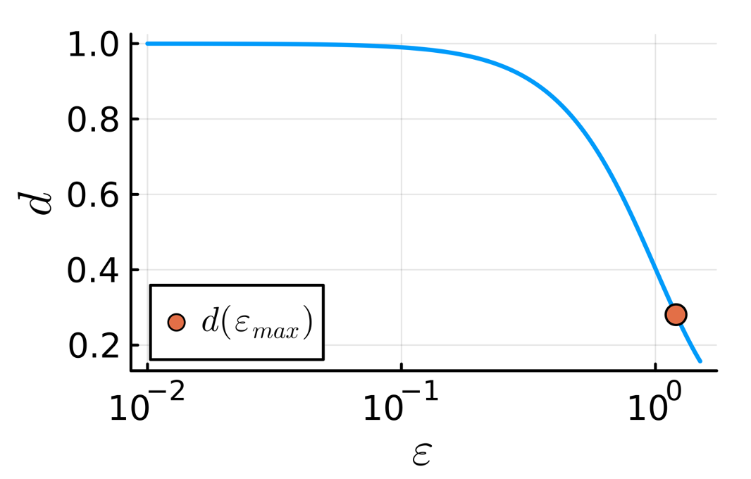
Figure 4: The measure of photon indistinguishability $d(\tilde{S}(\epsilon))$ (Eq. (39)) as a function of the perturbation strength $\epsilon$ [22]. This measure decreases monotonically with $\epsilon$ contrary to the behavior of the multimode bunching probability $P_{n}(\tilde{S}(\epsilon))$, which increases for $0\leq\epsilon\leq\epsilon_{max}$.

5 Decreasing bunching via small perturbations

So far we have established that a small perturbation to indistinguishable bosons can surprisingly increase bunching probabilities in some specific setups. In order to have a better understanding of the sensitivity of bunching probabilities to small perturbations we investigate another related question: given a state of indistinguishable bosons, what is the perturbation that leads to the maximum decrease of bunching effects?

Naively, one could expect that such a perturbation should take the internal states of the bosons towards a state of fully distinguishable particles corresponding to mutually orthogonal internal states. Similarly to the often-used model of partial distinguishability that interpolates between indistinguishable and distinguishable particles (see, for example, Ref. [4]) we can describe such a perturbation using the following parametrization of the bosons’ internal states

$$|\tilde{\phi_{i}}\rangle=\sqrt{1-\frac{\epsilon^{2}}{n}}\left|{\phi_{0}}\right\rangle+\frac{\epsilon}{\sqrt{n}}\left|{\eta_{i}}\right\rangle,$$ (40)

where the states $\left|{\eta_{i}}\right\rangle$ are orthogonal to $\left|{\phi_{0}}\right\rangle$ and also mutually orthogonal. Hence, the Gram matrix associated to the perturbation $\Delta_{ij}=\left\langle{\eta_{i}}\middle|{\eta_{j}}\right\rangle=\delta_{i,j}$ is the identity matrix. This perturbation takes the same form as that of Eq. (8) if we neglect terms of $O(\epsilon^{4})$ and choose $v_{i}=1/\sqrt{n},~{}\forall i$. We note that at $\epsilon=\sqrt{n}$ the internal states of the bosons become orthogonal, corresponding to fully distinguishable particles, but we are interested in small values of $\epsilon$. With a similar treatment to that of Sec. 3.2, namely using Eq. (3.2), we can show that the variation of the bunching probability is given by

$$\delta P_{n}\approx\epsilon^{2}\left(\frac{\text{tr}(F)}{n}-\text{perm}\left({H}\right)\right).$$ (41)

Alternatively, let us consider a different perturbation, which changes each boson state in the two dimensional space spanned by the orthogonal states $\{\left|{\phi_{0}}\right\rangle,\left|{\phi_{1}}\right\rangle\}$.

$$|\tilde{\phi_{i}}\rangle=\sqrt{1-\epsilon^{2}|{(v_{\min})}_{i}|^{2}}\left|{\phi_{0}}\right\rangle+\epsilon~{}{(v_{\min})}_{i}\left|{\phi_{1}}\right\rangle,~{}$$ (42)

where $\bm{v}_{min}$ is the eigenvector of $F$ corresponding to its lowest eigenvalue. The variation of the bunching probability is now described by Eq. (32) and yields

$$\delta P_{n}\approx\epsilon^{2}\left(\lambda_{min}(F)-\text{perm}\left({H}\right)\right).$$ (43)

Similarly to the proof of the upper bound in Eq. (31), it can be shown that the previously described perturbation attains the lower bound for the lowest possible value of $\delta P_{n}$, for the family of perturbations described in Sec. 3.2 (see Appendix D). Consequently, the perturbation described by in Eq. (40) leads to a less significant decrease in bunching probabilities than the one described by Eq. (42), even though the latter only changes the photons internal states in a two-dimensional subspace which is not enough to describe states of $n$ fully distinguishable photons. This result further highlights that care must be taken when trying to infer how distinguishable the photons are from a measurement of bunching probabilities.

6 Conclusion

The central result of this work is the identification of an optical circuit and a perturbation which, when applied to the state of perfectly indistinguishable bosons, enhances the probability for all bosons to bunch into two output modes. While it was already known that indistinguishable bosons do not necessarily always maximize multimode bunching probabilities [12], it remained quite plausible that this ideal situation describes at least a local maximum. However, the counterexample revealed in this paper shows that this state of indistinguishable bosons does not even locally maximize the multimode bunching probability. It would be interesting to identify the physical mechanism responsible for the enhancement of bunching with nearly indistinguishable bosons, as was previously done for the anomalous bunching effect found in Ref. [12]. Unfortunately, the mathematical counterexample of conjecture M2 exploited in the present work seems to be less structured than the counterexample of conjecture M1 exploited in [12], and consequently so does its physical realization as a linear optical experiment. A possible direction for future investigation is to try to find simpler scenarios (involving less than 8 photons) where such an effect could appear in a more pronounced way, as this would bring it closer to an experimental implementation and would potentially improve our understanding of this phenomenon.

We have also unveiled another counterintuitive behavior of the sensitivity of bunching probabilities to photon distinguishability, showing that a specific perturbation to the photonic wavefunctions in a two-dimensional space is the one that decreases bunching probabilities the most when compared to any other perturbation, possibly involving many more degrees of freedom. This implies that a perturbation going towards fully distinguishable photons is not the best way to decrease the multimode bunching probability starting from indistinguishable photons.

Despite the existence of several kinds of anomalous bunching phenomena as found in this work as well as Ref. [12], we believe that multimode bunching probabilities can be useful quantities to measure experimentally as witnesses of particle indistinguishability in many practical scenarios. Hence, we hope our work will inspire new research towards clarifying in which physical situations the observation of multimode bunching qualifies as a faithful indistinguishability witness.

Code availability

The numerical simulations were done using the package Permanents.jl [24, 25]. The source code generating the figures and data of this paper is available on github.

Appendix A Counterexamples for $|\mathcal{K}|\geq n$

In this appendix, we show how counterexamples to P1 with $|\mathcal{K}|<n$ can be trivially extended to counter-examples with $|\mathcal{K}|\geq n$. Consider a circuit $U_{1}$ with $n_{1}$ inpinging photons who violate P1 for some choice of internal wavefunctions $\left|{\phi_{1}}\right\rangle,...,\left|{\phi_{n_{1}}}\right\rangle$ and of subset $\mathcal{K}_{1}$ (see Fig. 5). To construct a counterexample with $|\mathcal{K}|\geq n$, we use the output modes of $U_{1}$ defined by $\mathcal{K}_{1}$ as inputs of a new network, $U_{2}$. The remaining modes of $U_{2}$ are populated by an input state $\hat{\rho}_{2}$, with $n_{2}$ single photons in a classically correlated or uncorrelated state . Considering all output modes of $U_{2}$ as a subset $\mathcal{K}_{2}$, we obtain a violation for the entire circuit ($U_{1},U_{2}$ combined as shown in Fig. 5). As long as $n=n_{1}+n_{2}\leq|\mathcal{K}_{2}|$ (for instance, by choosing $\hat{\rho}_{2}$ as the vacuum), we obtain a counterexample with less photons than the size of the subset ($\mathcal{K}=\mathcal{K}_{2}$). We also note that, even though in this construction the total interferometer $U$ does not couple all input modes to all output modes, it has been previously shown that violations to conjecture P1 exhibit a certain robustness to perturbations of the matrix elements of $U$ [12]. Hence, it should be possible to find counterexamples not only with $|\mathcal{K}|>n$ but also where all matrix elements describing the linear interferometer are non-zero.

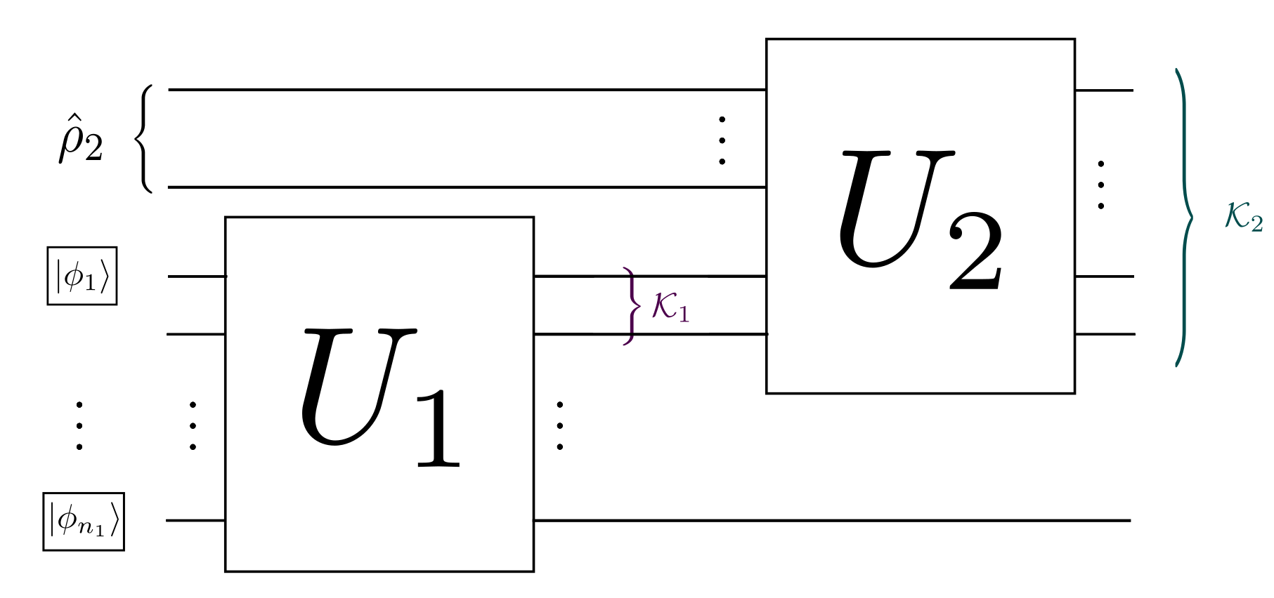
Figure 5: Counterexamples with $|\mathcal{K}|<n$ can be trivially extended to counter-examples with $|\mathcal{K}|\geq n$ by encompassing them in a larger circuit.

Appendix B Minc’s formula

Using Minc’s formula [26], it is possible to expand the permanent of the sum of two matrices, $A$ and $B$, as follows:

$$\text{perm}\left({A+B}\right)=$$

$$\sum_{r=0}^{n}\sum_{\alpha,\beta\in Q_{r,n}}\text{perm}\left({A[\alpha,\beta]}\right)\text{perm}\left({B(\alpha,\beta)}\right),$$ (44)

If $\Gamma_{r,n}$ is defined as the set of all $n^{r}$ sequences $u=\left(u_{1},\ldots,u_{r}\right)$ of integers, with $1\leq u_{i}\leq n,i=1,\ldots,n$, $Q_{r,n}$ is the set of increasing sequences defined as

$$Q_{r,n}=\left\{\left(u_{1},\ldots,u_{r}\right)\in\Gamma_{r,n}\mid 1\leq u_{1}<\cdots<u_{r}\leq n\right\}.$$ (45)

Furthermore, $A[\alpha,\beta]$ represents the $r\times r$ matrix formed by selecting the rows and columns of matrix $A$ based on the sets $\alpha$ and $\beta$. Conversely, $A(\alpha,\beta)$ denotes the $(n-r)\times(n-r)$ matrix obtained after excluding the rows and columns specified by $\alpha$ and $\beta$ from $A$.

Appendix C Connecting conjectures M1 and M2

In this appendix, we demonstrate that the validity of conjecture M1 would imply the validity of conjecture M2. Equivalently, we demonstrate that any counter-example disproving Conjecture M2 can be employed to construct a counterexample that also invalidates Conjecture M1. Even though both conjectures are known to be false this result implies an implication relation between properties of p.s.d. matrices: if the p.s.d. matrix $A$ is such that it obeys the statement of conjecture M1 for any p.s.d. matrix $B$ then $A$ also fulfills the statement of conjecture M2. We note that the opposite is not true, as can easily be tested with the example from Ref. [14] which obeys M2 but not M1.

This result follows a similar derivation as in Sec. 3.2 but we expose it here without using any physics terminology so it is more easily accessible to a broader community of researchers. In this section all calculations will follow the notation commonly utilized in mathematics, including the notation for conjugate transpose of a matrix $M$ which in the main text was denoted as $M^{\dagger}$ and here is denoted as $M^{*}$.

Let us denote by $\mathbf{H_{n}}$ the set of $n\times n$ positive semidefinite matrices. Moreover, let us define an $n$-dimensional complex vector $\bm{v}$, with $||\bm{v}||_{2}=1$, and a $n\times n$ correlation matrix $B(\epsilon)=M^{*}(\epsilon)M(\epsilon)$, with

$$M(\epsilon)=\left(\begin{array}[]{cccccccc}\frac{1}{\alpha_{1}}&\frac{1}{\alpha_{2}}&...&\frac{1}{\alpha_{n}}\\ \epsilon\frac{v_{1}}{\alpha_{1}}&\epsilon\frac{v_{2}}{\alpha_{2}}&...&\epsilon\frac{v_{n}}{\alpha_{n}}\\ \end{array}\right),$$ (46)

where $\epsilon\geq 0$. Here, $v_{i}$ is the $i$-th component of the vector $\bm{v}$ and $\alpha_{i}=\frac{1}{\sqrt{1+\epsilon^{2}|v_{i}|^{2}}}$ so that the 2-norm of all the column vectors of $M$ is equal to $1$. Note that $B(0)=\mathbb{E}$, which is the matrix whose entries are all $1$. The result of this section is the following.

Theorem 1.

Consider two matrices $A,B(\epsilon)\in\mathbf{H_{n}}$ with the correlation matrix $B(\epsilon)=M^{*}(\epsilon)M(\epsilon)$ defined as above. For $\epsilon>0$ the expansion of $\text{perm}\left({A\odot B(\epsilon)}\right)$ around $\epsilon=0$ is given by $\text{perm}\left({A\odot B(\epsilon)}\right)=\text{perm}\left({A}\right)+\epsilon^{2}(v^{*}Fv-\text{perm}\left({A}\right))+O(\epsilon^{4})$.

The implication between Mathematical Conjecture M2 and Mathematical Conjecture M1 is a corollary of this theorem.

Corollary 1.

Let $A\in\mathbf{H_{n}}$ be such that the largest eigenvalue of $F_{i,j}=A_{i,j}\text{perm}\left({A(i,j)}\right)$ is strictly greater than $\text{perm}\left({A}\right)$. By choosing $\bm{v}$ to be the eigenvector corresponding to the largest eigenvalue of $F$ we have that for some $\epsilon_{max}>0$

$$\text{perm}\left({A\odot B(\epsilon)}\right)>\text{perm}\left({A}\right),$$ (47)

for $0<\epsilon<\epsilon_{max}$.

Let us start by proving Theorem 1. By defining the matrix $B(\epsilon)$ as at the beginning of this section, we can expand the matrix around $\epsilon=0$,

$$B_{i,j}(\epsilon)=\frac{1}{\alpha_{i}\alpha_{j}}(1+\epsilon^{2}v_{i}^{*}v_{j})=1+\epsilon^{2}(v_{i}^{*}v_{j}-\frac{|v_{i}|^{2}}{2}-\frac{|v_{j}|^{2}}{2})+O(\epsilon^{4}).$$ (48)

To simplify the notations, it is useful to define the matrix $X_{i,j}=v_{i}^{*}v_{j}-\frac{|v_{i}|^{2}}{2}-\frac{|v_{j}|^{2}}{2}$ which allows us to express the matrix $B$ as

$$B=\mathbb{E}+\epsilon^{2}X+O(\epsilon^{4}).$$ (49)

With $\mathbb{E}_{i,j}=1$ for all $i,j$. This implies that

$$\text{perm}\left({A\odot B}\right)=\text{perm}\left({A\odot(\mathbb{E}+\epsilon^{2}X)}\right)+O(\epsilon^{4})=\text{perm}\left({A+\epsilon^{2}(A\odot X)}\right)+O(\epsilon^{4}).$$

Using a formula from Minc [26] for the permanent of the sum of two matrices (see Appendix A). We obtain

$$\text{perm}\left({A\odot B}\right)=\text{perm}\left({A}\right)+\epsilon^{2}\sum_{i,j}^{n}(A\odot X)_{i,j}\text{perm}\left({A(i,j)}\right)+O(\epsilon^{4}).$$ (50)

Let us focus on the term proportional to $\epsilon^{2}$, which can be written as

$$\sum_{i,j}^{n}(A\odot X)_{i,j}\text{perm}\left({A(i,j)}\right)=\sum_{i,j}^{n}X_{i,j}F_{i,j}=\sum_{i,j}^{n}(v_{i}^{*}v_{j}-\frac{|v_{i}|^{2}}{2}-\frac{|v_{j}|^{2}}{2})F_{i,j}=\sum_{i,j}^{n}v_{i}^{*}F_{i,j}v_{j}-\sum_{i,j}^{n}\frac{|v_{i}|^{2}}{2}F_{i,j}-\frac{|v_{j}|^{2}}{2}F_{i,j}.$$ (51)

Using the fact that $\sum_{i}^{n}F_{i,j}=\sum_{j}^{n}F_{i,j}=\text{perm}\left({A}\right)$ for every $i$ and $j$, and that $||\bm{v}||_{2}=1$, we have that

$$\sum_{i,j}^{n}X_{i,j}F_{i,j}=\bm{v}^{*}F\bm{v}-\text{perm}\left({A}\right).$$ (52)

Replacing this expression in Eq. (50) we prove that

$$\text{perm}\left({A\odot B(\epsilon)}\right)=\text{perm}\left({A}\right)+\epsilon^{2}(\bm{v}^{*}F\bm{v}-\text{perm}\left({A}\right))+O(\epsilon^{4}),$$ (53)

Which is the statement of Theorem 1. Then a counter-example to Conjecture M2 ($A$ and $\bm{v}$ such that $\bm{v}^{*}F\bm{v}>\text{perm}\left({A}\right)$ ) can be used to construct counter-examples to Conjecture M1, within some interval $\epsilon\in(0,\epsilon_{max})$. Although we have not done so, one could obtain a value for $\epsilon_{max}$ by upper bounding the term proportional to $\epsilon^{4}$ in Eq. (53).

Appendix D Minimization of bunching

As before, to determine the specific type of perturbation that minimizes the bunching of the indistinguishable state, we will seek a lower bound of $P_{n}(\tilde{S})$ and demonstrate that this bound is reached. To achieve this, we will analyze the following term

$$\delta P_{n}=\epsilon^{2}\Bigl{(}\sum_{k=1}^{K}(\bm{v}\odot\bm{u^{k}})^{\dagger}F(\bm{v}\odot\bm{u^{k}})-\text{perm}\left({H}\right)\Bigl{)}+O(\epsilon^{4}).$$

Let us define $\lambda_{min}(F)$ as the minimal eigenvalue of $F$. We will also introduce the family of vector $\bm{w^{k}}$, which are eigenvectors of $F$ associated with $\lambda_{min}(F)$ such that $||\bm{w}^{k}||=||\bm{v}\odot\bm{u}^{k}||$. We have

$$\sum_{k=1}^{K}(\bm{v}\odot\bm{u^{k}})^{\dagger}F(\bm{v}\odot\bm{u^{k}})\geq\sum_{k=1}^{K}(\bm{w}^{k})^{\dagger}F(\bm{w}^{k}).$$ (54)

Since $\bm{w}^{k}$ is an eigenvector of $F$ and by using Eq.(29), we have

$$\sum_{k=1}^{K}(\bm{w}^{k})^{\dagger}F(\bm{w}^{k})=\lambda_{min}\sum_{k=1}^{K}{||\bm{w}^{k}||^{2}}=\lambda_{min}(F).$$ (55)

The lower bound on $\delta P_{n}$ is, then

$$\delta P_{n}\geq\epsilon^{2}(\lambda_{min}(F)-\text{perm}\left({H}\right))+O(\epsilon^{4}).$$ (56)

As before, we note that this bound is reached in the case where the total Hilbert space has a dimension of $2$, and $\bm{v}$ is chosen to be the eigenvector of the matrix $F$ with the smallest eigenvalue. In this situation, the bunching is decreased by an amount of $\epsilon^{2}(\lambda_{\min}(F)-\text{perm}\left({H}\right)+O(\epsilon^{4})$ with the perturbation. This result is counterintuitive if we interpret the bunching as a direct consequence of indistinguishability, as this value is lower than the result presented in Eq. (41).

Appendix E Positive-semidefiniteness of $F$

Let us show that the matrix $F$ defined in Eq. (16) is positive semidefinite (p.s.d.). Let us write

$$F_{i,j}=(H\odot B)_{i,j},$$ (57)

with $B_{i,j}=\text{perm}\left({H(i,j)}\right).$ To show positive semidefiniteness, it suffices to show that the matrix $B$ is p.s.d.. Indeed as $H$ is p.s.d., we have $H\odot B$ being p.s.d. as well using Schur’s Theorem (see Theorem 7.21 on page 234 of [27]).

We recall a formalism from the book on permanents of Minc (see section 2.2. of [26]). Consider a matrix $H_{ij}=\left\langle{u_{i}}\middle|{v_{j}}\right\rangle$ whose the generating vectors $\bm{u_{1}},\dots,\bm{u_{n}},\bm{v_{1}},\dots,\bm{v_{n}}$ belong in a n-dimensional unitary space $V$. We write the tensor products of the generating vectors as $\bm{u_{1}}\otimes...\otimes\bm{u_{n}}\in V^{n}$. We introduce a scalar product on $V^{n}$

$$(\bm{u_{1}}\otimes...\otimes\bm{u_{n}},\bm{v_{1}}\otimes...\otimes\bm{v_{n}})=\prod_{i=1}^{n}\left\langle{u_{i}}\middle|{v_{i}}\right\rangle$$

as well as the completely symmetric operator

$$T_{n}=\frac{1}{n!}\sum_{\sigma\in S_{n}}P(\sigma),$$

with $P(\sigma)$ the permutation operator on $V^{n}$ corresponding to the permutation $\sigma$ :

$$P(\sigma)\left(\bm{u}_{1}\otimes\cdots\otimes\bm{u}_{n}\right)=\bm{u_{\sigma^{-1}(1)}}\otimes\cdots\otimes\bm{u_{\sigma^{-1}(n)}},$$

Defining the symmetric product

$$\bm{u_{1}}*...*\bm{u_{n}}=T_{n}(\bm{u_{1}}\otimes...\otimes\bm{u_{n}}),$$

Minc shows that

$$\text{perm}\left({H}\right)=(\bm{u_{1}}*...*\bm{u_{n}},\bm{v_{1}}*...*\bm{v_{n}}).$$

We apply this formalism to our case. As $H$ is a Gram matrix, $H_{ij}=\left\langle{u_{i}}\middle|{u_{j}}\right\rangle$ and its permanental cofactors are

$$\text{perm}\left({H(i,j)}\right)=(\bm{u_{1}}*...*\bm{\hat{u}_{i}}*...*\bm{u_{n}},\bm{u_{1}}*...*\bm{\hat{u}_{j}}*...*\bm{u_{n}}),$$

where $\hat{u}_{i}$ indicates that this vector id excluded from the product. Given this decomposition, we see that the matrix $B_{i,j}=\text{perm}\left({H(i,j)}\right)$ has its elements defined by a scalar product and is thus positive semidefinite.

References

- [1] E. Pelucchi, G. Fagas, I. Aharonovich, D. Englund, E. Figueroa, Q. Gong, H. Hannes, J. Liu, C.-Y. Lu, N. Matsuda, et al. The potential and global outlook of integrated photonics for quantum technologies. Nature Reviews Physics, 4(3):194–208, 2022.
- [2] H.-S. Zhong, H. Wang, Y.-H. Deng, M.-C. Chen, L.-C. Peng, Y.-H. Luo, J. Qin, D. Wu, X. Ding, Y. Hu, et al. Quantum computational advantage using photons. Science, 370(6523):1460–1463, 2020.
- [3] S. Aaronson and A. Arkhipov. The computational complexity of linear optics. In Proceedings of the forty-third annual ACM symposium on Theory of computing, pages 333–342, 2011.
- [4] M. C. Tichy. Sampling of partially distinguishable bosons and the relation to the multidimensional permanent. Physical Review, 91(2):022316, 2015.
- [5] V. S. Shchesnovich. Partial indistinguishability theory for multiphoton experiments in multiport devices. Physical Review A, 91(1):013844, 2015.
- [6] C.-K. Hong, Z.-Y. Ou, and L. Mandel. Measurement of subpicosecond time intervals between two photons by interference. Physical Review Letters, 59(18):2044, 1987.
- [7] N. Spagnolo, C. Vitelli, L. Sansoni, E. Maiorino, P. Mataloni, F. Sciarrino, D. J. Brod, Ernesto F. Galvão, A. Crespi, R. Ramponi, and R. Osellame. General rules for bosonic bunching in multimode interferometers. Physical Review Letters, 111:130503, 2013.
- [8] J. Carolan, P. J Meinecke, J. D. A.and Shadbolt, N. J. Russell, N. Ismail, K. Wörhoff, T. Rudolph, M. G. Thompson, J. L. O’brien, J. C. F. Matthews, et al. On the experimental verification of quantum complexity in linear optics. Nature Photonics, 8(8):621–626, 2014.
- [9] V. S. Shchesnovich. Universality of generalized bunching and efficient assessment of boson sampling. Physical Review Letters, 116(12):123601, 2016.
- [10] A. W. Young, S. Geller, W. J. Eckner, N. Schine, S. Glancy, E. Knill, and A. M. Kaufman. An atomic boson sampler. arXiv:2307.06936, 2023.
- [11] B. Seron, L. Novo, A. Arkhipov, and N. J. Cerf. Efficient validation of boson sampling from binned photon-number distributions. arXiv:2212.09643, 2022.
- [12] B. Seron, L. Novo, and N. J. Cerf. Boson bunching is not maximized by indistinguishable particles. Nature Photonics, 17(8):702–709, 2023.
- [13] R. B. Bapat and V. S. Sunder. On majorization and schur products. Linear algebra and its applications, 72:107–117, 1985.
- [14] S. Drury. A counterexample to a question of bapat and sunder. The Electronic Journal of Linear Algebra, 31:69–70, 2016.
- [15] R. B. Bapat and V. S. Sunder. An extremal property of the permanent and the determinant. Linear Algebra and its Applications, 76:153–163, 1986.
- [16] S. Drury. A counterexample to a question of Bapat & Sunder. Mathematical Inequalities & Applications, 21(2):517–520, 2018.
- [17] I. M. Wanless. Lieb’s permanental dominance conjecture. arXiv:2202.01867v1, 2022.
- [18] C. Dittel, G. Dufour, M. Walschaers, G. Weihs, A. Buchleitner, and R. Keil. Totally destructive many-particle interference. Physical Review Letters, 120(24):240404, 2018.
- [19] W. R. Clements, P. C. Humphreys, B. J. Metcalf, W. S. Kolthammer, and I.A. Walmsley. Optimal design for universal multiport interferometers. Optica, 3(12):1460–1465, 2016.
- [20] F. Zhang. Notes on hadamard products of matrices. Linear and Multilinear Algebra, 25(3):237–242, 1989.
- [21] V. S. Shchesnovich. The permanent-on-top conjecture is false. Linear Algebra and its Applications, 490:196–201, 2016.
- [22] V. S. Shchesnovich. Tight bound on the trace distance between a realistic device with partially indistinguishable bosons and the ideal bosonsampling. Physical Review A, 91(6):063842, 2015.
- [23] G.H. Gloub and Charles F. Van L. Matrix computations. Johns Hopkins Universtiy Press, 3rd edtion, 1996.
- [24] B. Seron. Permanents.jl: A Julia package for computing permanents, 2023. Available at Permanents.jl.
- [25] B. Seron and A. Restivo. Bosonsampling. jl: A Julia package for quantum multi-photon interferometry. arXiv:2212.09537, 2022.
- [26] H. Minc. Permanents. Cambridge University Press, 1984.
- [27] F. Zhang. Matrix theory: basic results and techniques. Springer Science & Business Media, 2011.