Physically Consistent Modelling of Wireless Links with Reconfigurable Intelligent Surfaces
Using Multiport Network Analysis

Abstract

RIS are an emerging technology for engineering the channels of future wireless communication systems. The vast majority of research publications on reconfigurable intelligent surface (RIS) are focussing on system-level optimization and are based on very simplistic models ignoring basic physical laws. There are only a few publications with a focus on physical modeling. Nevertheless, the widely employed model is still inconsistent with basic physical laws. We will show that even with a very simple abstract model based on isotropic radiators, ignoring any mismatch, mutual coupling, and losses, each RIS element cannot be modeled to simply reflect the incident signal by manipulating its phase only and letting the amplitude unchanged. We will demonstrate the inconsistencies with the aid of very simple toy examples, even with only one or two RIS elements. Based on impedance parameters, the problems associated with scattering parameters can be identified enabling a correct interpretation of the derived solutions.

This work has been submitted to the IEEE for possible publication. Copyright may be transferred without notice, after which this version may no longer be accessible.

I Introduction

I-A Background and related work

RISs are intended to engineer the propagation environment to improve the performance of wireless communications, especially in situations where the direct link between the transmit side (Tx) and receive side (Rx) is more or less blocked. Since many publications about RIS elaborate on why this is an interesting and promising technology [1], [2], we will not repeat this reasoning here but focus on the physically consistent modeling process and its consequences for the system optimization.

While most research has been performed on system-level optimization, e.g., [3], where over-simplistic models have been used, only a few publications are incorporating basic physical laws in the modeling process [4], [5]. Surprisingly, in these two publications, different approaches to modeling have been adopted. In [4], the analysis is based on impedance parameters, while in [5], a scattering parametrization has been chosen. One can argue which approach is, so to speak, the ”better” one. We will show that this is a matter of taste and may be convenience. In the impedance parameter approach, the variables are voltages and currents, while in the scattering parameter approach, the variables are incident and reflected waves. Since these two pairs of variables are simply related to each other by a linear transformation, the impedance matrices and the corresponding scattering matrices can easily be converted from one to the other. But interestingly enough, the results given in [4] and [5] finally lead to different conclusions.

Even in the simplest end-to-end single-input single-output (SISO) link with a blocked direct channel between Tx and Rx, the results in [5] suggest that the reactive terminations of the RIS elements change the phase of the signal received by each element and transmit it to the Rx without any change in amplitude, see (41)-(44) in [5, Section IV]. On the other hand, we learn from (12) in [4] that any change of that same reactive termination will change the phase and amplitude of the signals sent to the final destination Rx simultaneously. Apparently, it is impossible that both results are true at the same time. Therefore, we have to go for a careful investigation to find out what is the inherent problem there.

We give one last comment concerning the choice of either scattering or impedance parameters. For measurements in the microwave range, of course, scattering parameters are to be preferred. All the available measurement equipment with sound reasons is based on this approach. But for theoretical derivations, we feel that impedance parameters are better suited and are providing deeper insight, as we will see in the subsequent investigations.

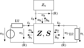
Figure 1: Multiport Model

I-B Contributions

We derive the multiport matrix of a RIS-aided multiple-input multiple-output (MIMO) link based on both impedance parameters and scattering parameters, neglecting all extrinsic and intrinsic noise sources. The conversion from impedance to scattering description and vice versa provides insight, especially on the relation of the direct link representation of the two results. Obviously, both approaches, correctly interpreted, lead to the same final result. However, there are interesting consequences for the channel estimation process if one chooses to follow the scattering parameter or the impedance parameter approach.

I-C Notation

Bold upper- and lower-case letters denote matrices and column vectors, respectively. $\bm{A}^{\mathrm{T}}$ and $\bm{A}^{{-1}}$ denote the transpose and the inverse of matrix $\bm{A}$, respectively. $\mathrm{j}=\sqrt{-1}$ is the imaginary unit. Scalars are non-bold letters, $|a|$, $\arg(a)$ are the magnitude and the phase of a complex scalar $a$. $\bm{\mathrm{I}}_{n}$ is the $n\times n$ identity matrix and $\bm{0}$ the all-zeros matrix.

II Multiport System Model

In this section, we firstly describe the basic assumptions about the antenna arrays used at Tx, Rx, and the RIS, that are incorporated in the multiport shown in Figure 1. This multiport can be characterized by its impedance matrix $\bm{Z}=\bm{Z}^{\mathrm{T}}$ (symmetric due to reciprocity), which is partioned as

$$\begin{bmatrix}\bm{v}_{\text{S}}\\ \bm{v}_{\text{R}}\\ \bm{v}_{\text{D}}\end{bmatrix}=\begin{bmatrix}\bm{Z}_{\text{S}}&\bm{Z}_{\text{SR}}&\bm{Z}_{\text{SD}}\\ \bm{Z}_{\text{RS}}&\bm{Z}_{\text{R}}&\bm{Z}_{\text{RD}}\\ \bm{Z}_{\text{DS}}&\bm{Z}_{\text{DR}}&\bm{Z}_{\text{D}}\\ \end{bmatrix}\begin{bmatrix}\bm{i}_{\text{S}}\\ \bm{i}_{\text{R}}\\ \bm{i}_{\text{D}}\end{bmatrix},$$ (1)

where $\bm{v}_{\text{S}}\in 1$\mathrm{V}$\cdot\mathbb{C}^{M},\bm{v}_{\text{R}}\in 1$\mathrm{V}$\cdot\mathbb{C}^{N},\text{ and }\bm{v}_{\text{D}}\in 1$\mathrm{V}$\cdot\mathbb{C}^{K},$ are the complex port voltages at the $M$ Tx antennas, $N$ RIS elements and $K$ Rx antennas, respectively, and $\bm{i}_{\text{S}},\bm{i}_{\text{R}},\text{ and }\bm{i}_{\text{D}}$ are the corresponding port currents. Equivalently, the multiport can be characterized by

$$\begin{bmatrix}\bm{b}_{\text{S}}\\ \bm{b}_{\text{R}}\\ \bm{b}_{\text{D}}\end{bmatrix}=\begin{bmatrix}\bm{S}_{\text{S}}&\bm{S}_{\text{SR}}&\bm{S}_{\text{SD}}\\ \bm{S}_{\text{RS}}&\bm{S}_{\text{R}}&\bm{S}_{\text{RD}}\\ \bm{S}_{\text{DS}}&\bm{S}_{\text{DR}}&\bm{S}_{\text{D}}\\ \end{bmatrix}\begin{bmatrix}\bm{a}_{\text{S}}\\ \bm{a}_{\text{R}}\\ \bm{a}_{\text{D}}\end{bmatrix}$$ (2)

where $\bm{a}_{\text{S}}$, $\bm{a}_{\text{R}}$, and $\bm{a}_{\text{D}}$ are the incident voltage waves and $\bm{b}_{\text{S}}$, $\bm{b}_{\text{R}}$, and $\bm{b}_{\text{D}}$ their reflected counterparts, which are related to the port voltages and currents by

$$\bm{v}_{\Gamma} =\bm{a}_{\Gamma}+\bm{b}_{\Gamma},\quad \bm{i}_{\Gamma} =(\bm{a}_{\Gamma}-\bm{b}_{\Gamma})/R,$$ (3)

where $\Gamma\in\{{\text{S}},{\text{R}},{\text{D}}\}$ refers to each of the ports, and $R$ is the port resistance, assigned to all ports. Additionally, the wave parameters are given by

$$\bm{a}_{\Gamma}=\frac{1}{2}(\bm{v}_{\Gamma}+R\bm{i}_{\Gamma}),\quad\bm{b}_{\Gamma}=\frac{1}{2}(\bm{v}_{\Gamma}-R\bm{i}_{\Gamma}).$$ (4)

We have assumed that the source impedances of the high power amplifier (HPA) outputs, which are connected to the Tx antennas, and the input impedances of the low noise amplifier (LNA) inputs, which are connected as a load to the Rx antennas are, without loss of generality, all of the same value $R$. For the $N$-port characterized by $\bm{Z}_{\text{N}}$ (see Fig 1), it is assumed that each RIS element is terminated with one reactive, i.e., lossless, one-port. The matrix $\bm{Z}_{\text{N}}$, therefore, is diagonal with imaginary entries.

Now we assume that all antenna elements at the Tx, RIS and Rx are isotropic radiators, although we know that such elements do not exist for vector fields. However, a field-theoretic justification for using such hypothetical elements is given in [6]. We’d like to note that almost in every system-level publication dealing with antenna arrays, such a model is used. The self-impedance is real-valued and is assumed to be equal to the port resistance $R$. Hence, we have power matching between the HPAs and Tx-antennas as well as the LNAs and Rx-antennas.

If no current is flowing across the terminals of an isotropic radiator, then this radiator does not produce any electromagnetic field, i.e., it is of the so-called canonic minimum scattering type [7].

The so-called effective area of an isotropic radiator is $A=\frac{\lambda^{2}}{4\pi}$ and the gain, which is uniform for all azimuth and elevation angles is $G=1$. The ratio between $A$ and $G$ is $\frac{\lambda^{2}}{4\pi}$, which is true for any antenna type [8, Chapter 13.7, pp. 569-575].

There is, of course, mutual coupling between isotropic radiators, which we can compute as

$$z_{21}=\frac{v_{2}}{i_{1}}\bigg{|}_{i_{2}=0$\mathrm{A}$}=-\frac{R}{\mathrm{j}kd}\mathrm{e}^{-\mathrm{j}kd},$$ (5)

where $k=\frac{2\pi}{\lambda}$ is the wave number, $d$ the distance between the antenna excited by current $i_{1}$ and the second open-circuited antenna, whose voltage $v_{2}$ is induced. Such a mutual impedance is necessary to have communication between Tx, RIS, and Rx. It exists, of course, also between antenna elements within the Tx-array, RIS and Rx-array and it will be incorporated by the off-diagonal entries of the matrices $\bm{Z}_{\text{S}}$, $\bm{Z}_{\text{R}}$, and $\bm{Z}_{\text{D}}$.

Now we follow Subsection III.B in [5] and analyze the RIS-aided communication model in Figure 1 with perfect matching and without intra-array coupling, resulting in the impedance matrices

$$\bm{Z}_{\text{S}} =\bm{\mathrm{I}}_{M}R,\quad \bm{Z}_{\text{R}} =\bm{\mathrm{I}}_{N}R,\quad \bm{Z}_{\text{D}} =\bm{\mathrm{I}}_{K}R$$ (6)

and the scattering matrices

$$\bm{S}_{\text{S}}=\bm{0},\quad\bm{S}_{\text{R}}=\bm{0},\quad\bm{S}_{\text{D}}=\bm{0}.$$ (7)

Because antennas and physical wireless channels are reciprocal, it is generally true that

$$\bm{Z}_{\text{SR}}=\bm{Z}_{\text{RS}}^{\mathrm{T}},\quad\bm{Z}_{\text{SD}}=\bm{Z}_{\text{DS}}^{\mathrm{T}},\quad\bm{Z}_{\text{RD}}=\bm{Z}_{\text{DR}}^{\mathrm{T}}.$$ (8)

However, it is also true that the signal attenuation between Tx and RIS, between RIS and Rx, as well as between Tx and Rx is usually very large. Hence,

$$\|\bm{Z}_{{\text{SR}}}\|_{\text{F}}\ll\|\bm{Z}_{{\text{S}}}\|_{\text{F}},\quad\|\bm{Z}_{{\text{SD}}}\|_{\text{F}}\ll\|\bm{Z}_{{\text{S}}}\|_{\text{F}},\quad\|\bm{Z}_{{\text{RD}}}\|_{\text{F}}\ll\|\bm{Z}_{{\text{R}}}\|_{\text{F}}$$ (9)

holds in practice. Therefore, we keep $\bm{Z}_{\text{RS}}$, $\bm{Z}_{\text{DS}}$ and $\bm{Z}_{\text{DR}}$ as they are and set

$$\bm{Z}_{\text{SR}}=\bm{0}\;$\mathrm{\SIUnitSymbolOhm}$,\quad\bm{Z}_{\text{SD}}=\bm{0}\;$\mathrm{\SIUnitSymbolOhm}$,\quad\bm{Z}_{\text{RD}}=\bm{0}\;$\mathrm{\SIUnitSymbolOhm}$,$$ (10)

which we call the unilateral approximation [9], [10]. For the scattering parameters, we have, accordingly,

$$\bm{S}_{\text{SR}}=\bm{0},\quad\bm{S}_{\text{SD}}=\bm{0},\quad\bm{S}_{\text{RD}}=\bm{0}.$$ (11)

This leads to the multiport impedance matrix

$$\bm{Z}=\begin{bmatrix}\bm{\mathrm{I}}R&\bm{0}&\bm{0}\\ \bm{Z}_{\text{RS}}&\bm{\mathrm{I}}R&\bm{0}\\ \bm{Z}_{\text{DS}}&\bm{Z}_{\text{DR}}&\bm{\mathrm{I}}R\\ \end{bmatrix}$$ (12)

as well as the multiport scattering matrix

$$\bm{S}=\begin{bmatrix}\bm{0}&\bm{0}&\bm{0}\\ \bm{S}_{\text{RS}}&\bm{0}&\bm{0}\\ \bm{S}_{\text{DS}}&\bm{S}_{\text{DR}}&\bm{0}\\ \end{bmatrix}.$$ (13)

From these assumptions and Figure 1 we obtain the voltages

$$\bm{v}_{\text{G}}=\bm{v}_{\text{S}}+\bm{\mathrm{I}}_{M}R\bm{i}_{\text{S}},\quad\bm{v}_{\text{R}}=-\bm{Z}_{\text{N}}\bm{i}_{\text{R}},\quad\bm{v}_{\text{D}}=-\bm{\mathrm{I}}_{K}R\bm{i}_{\text{D}}=\bm{v}_{\text{L}}$$ (14)

as well as the scattering parameters

$$\bm{a}_{\text{S}}=\frac{1}{2}\bm{v}_{\text{G}},\quad\bm{a}_{\text{R}}=\bm{\Theta}\bm{b}_{\text{R}},\quad\bm{a}_{\text{D}}=\bm{0}$\mathrm{V}$,\quad\bm{b}_{\text{S}}=\bm{0}$\mathrm{V}$.$$ (15)

Additionally, we have

$$\bm{b}_{\text{D}}=\bm{v}_{\text{D}}=\bm{v}_{\text{L}}\quad\text{and}\quad\bm{\Theta}=(\bm{Z}_{\text{N}}-\bm{\mathrm{I}}R)(\bm{Z}_{\text{N}}+\bm{\mathrm{I}}R)^{{-1}}$$ (16)

where $\bm{\Theta}$ is a diagonal matrix with unit-modulus constraints as $\bm{Z}_{\text{N}}$ is assumed to be diagonal and purely imaginary.

From here and since $\bm{v}_{\text{G}}=2\bm{v}_{\text{S}}=2R\bm{i}_{\text{S}}$ we compute the transfer matrix based on the impedance parameters as

$$\bm{v}_{\text{L}}=\bm{D}\bm{v}_{\text{G}},\quad\bm{D}=\frac{1}{4R}\left(\bm{Z}_{\text{DS}}-\bm{Z}_{\text{DR}}(\bm{Z}_{\text{N}}+\bm{\mathrm{I}}R)^{-1}\bm{Z}_{\text{RS}}\right)$$ (17)

and based on the scattering parameters as

$$\bm{b}_{\text{D}}=\bm{H}2\bm{a}_{\text{S}},\quad\bm{H}=\frac{1}{2}(\bm{S}_{\text{DS}}+\bm{S}_{\text{DR}}\bm{\Theta}\bm{S}_{\text{RS}}).$$ (18)

From (16), we have $\bm{b}_{\text{D}}=\bm{v}_{\text{L}}$ and $2\bm{a}_{\text{S}}=\bm{v}_{\text{G}}$. Therefore $\bm{H}$ and $\bm{D}$ must be identical! We will validate that by using the standard relationships

$$\bm{S}=(\bm{Z}-\bm{\mathrm{I}}R)(\bm{Z}+\bm{\mathrm{I}}R)^{-1}\text{ and }\bm{Z}=R(\bm{\mathrm{I}}+\bm{S})(\bm{\mathrm{I}}-\bm{S})^{-1}$$ (19)

which follow directly from (3) and (4). In particular, with

$$(\bm{Z}-\bm{\mathrm{I}}R)=\bm{S}(\bm{Z}+\bm{\mathrm{I}}R),$$ (20)

it can be shown that

$$\bm{S}_{\text{RS}}=\frac{1}{2R}\bm{Z}_{\text{RS}},\;\bm{S}_{\text{DR}}=\frac{1}{2R}\bm{Z}_{\text{DR}}\quad\text{and}$$ (21)

$$\bm{S}_{\text{DS}}=\frac{1}{2R}\left(\bm{Z}_{\text{DS}}-\frac{1}{2R}\bm{Z}_{\text{DR}}\bm{Z}_{\text{RS}}\right).$$ (22)

It is important to note, that the result in (22) is different from (37) in [5]. Using (22) to compare (17) and (18), we confirm $\bm{D}=\bm{H}$. Nevertheless, let us consider the case of a weak or even fully blocked direct link between Tx and Rx. From (17) we get with $\bm{Z}_{\text{DS}}=\bm{0}$\mathrm{\SIUnitSymbolOhm}$$,

$$\bm{D}_{0}=\bm{D}|_{\bm{Z}_{\text{DS}}=\bm{0}$\mathrm{\SIUnitSymbolOhm}$}=-\frac{1}{4R}\bm{Z}_{{\text{DR}}}(\bm{Z}_{\text{N}}+\bm{\mathrm{I}}R)^{-1}\bm{Z}_{\text{RS}},$$ (23)

while setting $\bm{S}_{\text{DS}}=\bm{0}$ in (18) would lead to

$$\bm{H}|_{\bm{S}_{\text{DS}}=\bm{0}}=\frac{1}{2}\bm{S}_{\text{DR}}\bm{\Theta}\bm{S}_{\text{RS}},$$ (24)

which obviously is different from $\bm{D}_{0}$! However, by using (22), we get

$$\bm{S}_{\text{DS}}^{0}=\bm{S}_{\text{DS}}|_{\bm{Z}_{\text{DS}}=\bm{0}$\mathrm{\SIUnitSymbolOhm}$}=-\bm{S}_{\text{DR}}\bm{S}_{\text{RS}}.$$ (25)

Substituting (25) into (18), we obtain

$$\bm{H}_{0} =\frac{1}{2}(-\bm{S}_{\text{DR}}\bm{S}_{\text{RS}}+\bm{S}_{\text{DR}}\bm{\Theta}\bm{S}_{\text{RS}})=\frac{1}{2}\bm{S}_{\text{DR}}(\bm{\Theta}-\bm{\mathrm{I}}_{N})\bm{S}_{\text{RS}}$$ (26)

$$=\frac{1}{2}\bm{S}_{\text{DR}}\Big{(}(\bm{Z}_{\text{N}}-\bm{\mathrm{I}}R)(\bm{Z}_{\text{N}}+\bm{\mathrm{I}}R)^{{-1}}$$

$$\quad-(\bm{Z}_{\text{N}}+\bm{\mathrm{I}}R)(\bm{Z}_{\text{N}}+\bm{\mathrm{I}}R)^{{-1}}\Big{)}\bm{S}_{\text{RS}}$$

$$=-\frac{1}{2}\bm{S}_{\text{DR}}\left(2\bm{\mathrm{I}}_{N}R(\bm{Z}_{\text{N}}+\bm{\mathrm{I}}R)^{-1}\right)\bm{S}_{\text{RS}}$$

$$=-\bm{S}_{\text{DR}}R(\bm{Z}_{\text{N}}+\bm{\mathrm{I}}R)^{-1}\bm{S}_{\text{RS}}$$

$$=-\frac{1}{4R}\bm{Z}_{\text{DR}}(\bm{Z}_{\text{N}}+\bm{\mathrm{I}}R)^{-1}\bm{Z}_{\text{RS}}=\bm{D}_{0},$$

which is now correct and identical to $\bm{D}_{0}$ from (23).

Therefore, the matrix in between $\bm{S}_{\text{DR}}$ and $\bm{S}_{\text{RS}}$ is not only changing the phase of the signals emitted from each RIS element, but simultaneously, the amplitude is changed. This important consequence has been overlooked in [5] and many other publications are based on the assumption in (37) of [5], which erroneously states that $\bm{S}_{\text{DS}}=\frac{1}{2R}\bm{Z}_{\text{DS}}$. A careful conversion between $\bm{S}$ and $\bm{Z}$ matrices shows the correct result in (22).

There is still the question why the intuitive reasoning in [5] is wrong. This is because in (24) the salient assumption is that only the waves $\bm{a}_{\text{R}}$, which are reflected by the reactive terminations, are propagating toward the final destination, i.e. the Rx. But at the ports of the RIS elements, we have not only $\bm{a}_{\text{R}}$, but the superposition of $\bm{a}_{\text{R}}$ and $\bm{b}_{\text{R}}$ simultaneously and therefore, this superposition of both is propagated towards the Rx. But the contribution of $\bm{b}_{\text{R}}$, which is not incorporated in the triple product $\bm{S}_{\text{DR}}\bm{\Theta}\bm{S}_{\text{DS}}$ has been moved to the element $\bm{S}_{\text{DS}}$ and has been overlooked there.

For the problem of channel estimation, we have to recognize that the three channel matrices $\bm{Z}_{\text{DS}}$, $\bm{Z}_{\text{RS}}$, and $\bm{Z}_{\text{DR}}$ are truly different and independent entities. The statistical fading processes of their random entries are uncorrelated and even statistically independent. On the contrary, if one tries to estimate $\bm{S}_{\text{DS}},\bm{S}_{\text{DR}}$ and $\bm{S}_{\text{RS}}$, it is important to note the deterministic dependency of $\bm{S}_{\text{DS}}$ on $\bm{S}_{\text{RS}}$ and $\bm{S}_{\text{DR}}$.

If somebody wants to use the entries of $\bm{\Theta}$ as optimization parameters instead of the entries of $\bm{Z}_{\text{N}}$, we can use the impedance parameter description equally well

$$\bm{D}=\frac{1}{4R}\left(\bm{Z}_{\text{DS}}-\frac{1}{2R}\bm{Z}_{\text{DR}}\bm{Z}_{\text{RS}}+\frac{1}{2R}\bm{Z}_{\text{DR}}\bm{\Theta}\bm{Z}_{\text{RS}}\right).$$ (27)

Summarizing the two main messages obtained from the above derivation, we have:

• A change of the lossless terminations of the RIS elements do not only change the phase of the signals propagating from the RIS to the Rx. The amplitude of said signals will unavoidably also be changed.

• Even when the direct link betweeen Tx and Rx is completely blocked, the scattering matrix $\bm{S}_{\text{DS}}=-\bm{S}_{\text{DR}}\bm{S}_{\text{RS}}$ is not equal to the zero matrix.

Next, we will show with extremely simple scenarios that ignoring the effect of the lossless terminations on the signal amplitudes is quite substantial.

III Numerical Results

III-A Single RIS Element

First, we will demonstrate the amplitude change with a line of sight (LOS)-SISO link with a single RIS element. We have $M=N=K=1$, and we assume a blocked direct link. In that scenario, we can easily observe that the amplitude of the signal received by the Rx will be quite different for different lossless terminations. We have

$$z_{\text{S}}=R,\;z_{\text{D}}=R,\;z_{\text{N}}=\mathrm{j}X,z_{\text{DS}}=0\;$\mathrm{\SIUnitSymbolOhm}$,$$ (28)

$$z_{\text{RS}}=\mathrm{j}\frac{R\lambda}{2\pi d_{\text{RS}}}e^{-\mathrm{j}2\pi\frac{d_{\text{RS}}}{\lambda}},\;z_{\text{DR}}=\mathrm{j}\frac{R\lambda}{2\pi d_{\text{DR}}}e^{-\mathrm{j}2\pi\frac{d_{\text{DR}}}{\lambda}}$$

and we choose $d_{\text{RS}}=10^{2}\lambda$ and $d_{\text{DR}}=10^{3}\lambda$. This leads to

$$D_{0}=\frac{1}{(4\pi)^{2}}10^{-5}\frac{R}{R+\mathrm{j}X}.$$ (29)

We normalize $D_{0}$ to take out the path loss and get

$$D_{0}^{\prime}=(4\pi)^{2}10^{5}D_{0}=\frac{1}{1+\mathrm{j}x},\quad x=\frac{X}{R}$$ (30)

as well as

$$\phi=\arg D_{0}^{\prime}=-\arctan x\;\text{ and }\;|D_{0}^{\prime}|=(1+x^{2})^{-\frac{1}{2}}.$$ (31)

We summarize the results for a number of different terminations in Table I.

$x$	$\phi/\circ$	$|D_{0}^{\prime}|$	$10\log_{10}|D^{\prime}_{0}|^{2}/$$\mathrm{d}\mathrm{B}$
$-\infty$	$90$	$0$	$-\infty$
$-1$	$45$	$\frac{1}{\sqrt{2}}$	$-3$
$0$	$0$	$1$	$0$
$1$	$-45$	$\frac{1}{\sqrt{2}}$	$-3$
$\infty$	$-90$	$0$	$-\infty$

TABLE I: Single RIS Element

There is quite a dramatic change in amplitude associated with the phase shift. Although in this example, any other phase shift than $\phi=0^{\circ}$ does not make any sense in the case of a single RIS element, this example already demonstrates the importance of the correct interpretation of the model.

III-B Two RIS Elements

Now we add a second element according to Figure 2.

Figure 2: SISO Link with Two-Element RIS

We normalize $D_{0}$ as before and get

$$D_{0}^{\prime}=\frac{1+\mathrm{j}x_{2}+e^{-\mathrm{j}2\pi\frac{d}{\lambda}}(1+\mathrm{j}x_{1})}{(1+\mathrm{j}x_{1})(1+\mathrm{j}x_{2})},$$ (32)

with $x_{1}=\frac{X_{1}}{R}$ and $x_{2}=\frac{X_{2}}{R}$ being the normalized reactances terminating the two RIS elements. Now we maximize $|D^{\prime}_{0}|$ to have the best possible signal at the Rx. In Table II we display the optimum reactances and the corresponding values of the normalized magnitude of the transfer function.

$d$	$x_{1}$	$x_{2}$	$|D_{0}^{\prime}|^{2}$	$10\log_{10}|D^{\prime}_{0}|^{2}/$$\mathrm{d}\mathrm{B}$
$0$	$0$	$0$	$4$	$6$
$\frac{\lambda}{4}$	$\sqrt{2}-1$	$1-\sqrt{2}$	$\frac{1}{6-4\sqrt{2}}$	$4,6$
$\frac{\lambda}{2}$	$1$	$-1$	$1$	$0$
$\frac{3\lambda}{4}$	$1-\sqrt{2}$	$\sqrt{2}-1$	$\frac{1}{6-4\sqrt{2}}$	$4,6$
$\lambda$	$0$	$0$	$4$	$6$

TABLE II: Optimum Design for the SISO link with a two-element RIS

It is important to note that an optimization based on section IV.A of [5] leads to a completely different result. The receive signal power would have been independent of the distance $d$ of the two RIS elements constant at $0$ $\mathrm{d}\mathrm{B}$.

It is important to note that the optimization result for this conventional model has a degree of freedom, i.e. one of the elements of the diagonal $\bm{\Theta}$ can be set to any arbitrary value, e.g. zero, without changing the achieved power gain. But this is true only, if the diagonal $\bm{\Theta}$ is applied to a system, which faithfully follows the conventional, but erroneous model (24). If this $\bm{\Theta}$ is appled to to a more realistic model, i.e. the physically consistent one (23), then the previously arbitrary choice is not arbitrary anymore and has quite an influence on the achieved power gain.

The whole picture is shown in Figure 3, where the curve with the blue circles show the achievable power gain as a function of the spacing between the two RIS elements. Here the optimization has been carried out on the physically consistent model (23) showing quite an improved performance compared to the conventional model, which is given by the red curve. In contrast, applying the optimization result obtained with the conventional model to physcally consistent one, we get an even worse power gain given by the curve with the green triangles. Here we have set the phase factor for the RIS element 1 to zero degrees. With other choices we can generate very many different curves.

As a baseline comparison there have been added two more curves, which are not optimization results but have been generated by averaging over many independently and uniformly distributed random phase realizations. Obviously, these results, given by dashed and dotted lines, are well below their optimized counterparts.

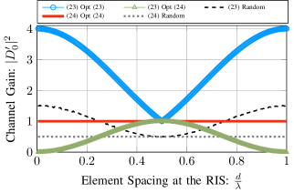
Figure 3: Model Comparison over Element Spacing

It is interesting to note that now the gain $|D_{0}^{\prime}|^{2}$ depends on the choice of the phase applied for the phase $\phi_{1}$ of RIS element numbered one. In the conventional model (24), this choice would have no effect on the gain, but in reality, it does.

IV Conclusion

The discrepancy of two different models for a RIS-aided communication link given in [4] and [5] has been resolved. This difference is most striking in the case of a blocked direct link, but even if this is not the case, we have to be careful in interpreting the different approaches in describing the same scenario correctly.

The important consequence of correct modeling has been demonstrated with a very simple toy scenario and by assuming isotropic radiators by ignoring intra-array mutual coupling.

What has been called physically consistent modelling was simply the correct separation of the direct link from the link via the RIS. There are a number of further steps ahead to achieve physial consistency in a broader sense. Obviously, future research has to focus on real-world scenarios with a large number of RIS elements, including intra-array mutual coupling, mismatch, and losses. For taking into account finite bandwidth, we must also proceed with real-world antenna elements instead of isotropic ones.

The fact that there are three different channel matrices, the one from Tx to the RIS, the one from the RIS to the Rx and eventually a direct link from Tx to Rx, have to be estimated, should be reconsidered. Whether this is based on impedance parameters or scattering parameters can make a difference. The same is true for expected values of achievable rates taking into account the statistical properties of the different channel matrices.

References

- [1] M. Di Renzo, A. Zappone, M. Debbah, M.-S. Alouini, C. Yuen, J. de Rosny, and S. Tretyakov, “Smart radio environments empowered by reconfigurable intelligent surfaces: How it works, state of research, and the road ahead,” IEEE Journal on Selected Areas in Communications, vol. 38, no. 11, pp. 2450–2525, 2020.
- [2] S. Gong, X. Lu, D. T. Hoang, D. Niyato, L. Shu, D. I. Kim, and Y.-C. Liang, “Toward smart wireless communications via intelligent reflecting surfaces: A contemporary survey,” IEEE Communications Surveys & Tutorials, vol. 22, no. 4, pp. 2283–2314, 2020.
- [3] B. Sihlbom, M. I. Poulakis, and M. D. Renzo, “Reconfigurable intelligent surfaces: Performance assessment through a system-level simulator,” IEEE Wireless Communications, pp. 1–10, 2022.
- [4] G. Gradoni and M. Di Renzo, “End-to-end mutual coupling aware communication model for reconfigurable intelligent surfaces: An electromagnetic-compliant approach based on mutual impedances,” IEEE Wireless Communications Letters, vol. 10, no. 5, pp. 938–942, 2021.
- [5] S. Shen, B. Clerckx, and R. Murch, “Modeling and architecture design of reconfigurable intelligent surfaces using scattering parameter network analysis,” IEEE Transactions on Wireless Communications, vol. 21, no. 2, pp. 1229–1243, 2022.
- [6] H. Yordanov, P. Russer, M. T. Ivrlač, and J. A. Nossek, “Arrays of isotropic radiators — a field-theoretic justification,” Proc. of the IEEE/ITG International Workshop on Smart Antennas, 2009.
- [7] W. Kahn and H. Kurss, “Minimum-scattering antennas,” IEEE Transactions on Antennas and Propagation, vol. 13, no. 5, pp. 671–675, 1965.
- [8] P. Russer, Electromagnetics, Microwave Circuit, and Antenna Design for Communications Engineering, ser. Artech House antennas and propagation library. Artech House, 2003.
- [9] M. T. Ivrlač and J. A. Nossek, “Toward a circuit theory of communication,” IEEE Transactions on Circuits and Systems I: Regular Papers, vol. 57, no. 7, pp. 1663–1683, 2010.
- [10] ——, “The multiport communication theory,” IEEE Circuits and Systems Magazine, vol. 14, no. 3, pp. 27–44, 2014.